Precise expressions for random projections:
Low-rank approximation and randomized Newton

Abstract

It is often desirable to reduce the dimensionality of a large dataset by projecting it onto a low-dimensional subspace. Matrix sketching has emerged as a powerful technique for performing such dimensionality reduction very efficiently. Even though there is an extensive literature on the worst-case performance of sketching, existing guarantees are typically very different from what is observed in practice. We exploit recent developments in the spectral analysis of random matrices to develop novel techniques that provide provably accurate expressions for the expected value of random projection matrices obtained via sketching. These expressions can be used to characterize the performance of dimensionality reduction in a variety of common machine learning tasks, ranging from low-rank approximation to iterative stochastic optimization. Our results apply to several popular sketching methods, including Gaussian and Rademacher sketches, and they enable precise analysis of these methods in terms of spectral properties of the data. Empirical results show that the expressions we derive reflect the practical performance of these sketching methods, down to lower-order effects and even constant factors.

1 Introduction

Many settings in modern machine learning, optimization and scientific computing require us to work with data matrices that are so large that some form of dimensionality reduction is a necessary component of the process. One of the most popular families of methods for dimensionality reduction, coming from the literature on Randomized Numerical Linear Algebra (RandNLA), consists of data-oblivious sketches [Mah11, HMT11, Woo14]. Consider a large $m\times n$ matrix $\mathbf{A}$. A data-oblivious sketch of size $k$ is the matrix $\mathbf{S}\mathbf{A}$, where $\mathbf{S}$ is a $k\times m$ random matrix such that $\mathbb{E}[\frac{1}{k}\mathbf{S}^{\scriptscriptstyle{\top}}\mathbf{S}]=\mathbf{I}$, whose distribution does not depend on $\mathbf{A}$. This sketch reduces the first dimension of $\mathbf{A}$ from $m$ to a much smaller $k$ (we assume without loss of generality that $k\ll n\leq m$), and an analogous procedure can be defined for reducing the second dimension as well. This approximate representation of $\mathbf{A}$ is central to many algorithms in areas such as linear regression, low-rank approximation, kernel methods, and iterative second-order optimization. While there is a long line of research aimed at bounding the worst-case approximation error of such representations, these bounds are often too loose to reflect accurately the practical performance of these methods. In this paper, we develop new theory which enables more precise analysis of the accuracy of sketched data representations.

A common way to measure the accuracy of the sketch $\mathbf{S}\mathbf{A}$ is by considering the $k$-dimensional subspace spanned by its rows. The goal of the sketch is to choose a subspace that best aligns with the distribution of all of the $m$ rows of $\mathbf{A}$ in $\mathbb{R}^{n}$. Intuitively, our goal is to minimize the (norm of the) residual when projecting a vector $\mathbf{a}\in\mathbb{R}^{n}$ onto that subspace, i.e., $\mathbf{a}-\mathbf{P}\mathbf{a}=(\mathbf{I}-\mathbf{P})\mathbf{a}$, where $\mathbf{P}=(\mathbf{S}\mathbf{A})^{\dagger}\mathbf{S}\mathbf{A}$ is the orthogonal projection matrix onto the subspace spanned by the rows of $\mathbf{S}\mathbf{A}$ (and $(\cdot)^{\dagger}$ denotes the Moore-Penrose pseudoinverse). For this reason, the quantity that has appeared ubiquitously in the error analysis of RandNLA sketching is what we call the residual projection matrix:

$$\textbf{(residual projection matrix)}\quad\mathbf{P}_{\!\perp}\ :=\ \mathbf{I}-\mathbf{P}\ =\ \mathbf{I}-(\mathbf{S}\mathbf{A})^{\dagger}\mathbf{S}\mathbf{A}.$$

Since $\mathbf{P}_{\!\perp}$ is random, the average performance of the sketch can often be characterized by its expectation, $\mathbb{E}[\mathbf{P}_{\!\perp}]$. For example, the low-rank approximation error of the sketch can be expressed as $\mathbb{E}[\|\mathbf{A}-\mathbf{A}\mathbf{P}\|_{F}^{2}]=\mathrm{tr}\,\mathbf{A}^{\scriptscriptstyle{\top}}\mathbf{A}\,\mathbb{E}[\mathbf{P}_{\!\perp}]$, where $\|\cdot\|_{F}$ denotes the Frobenius norm. A similar formula follows for the trace norm error of a sketched Nyström approximation [WS01, GM16]. Among others, this approximation error appears in the analysis of sketched kernel ridge regression [FSS20] and Gaussian process regression [BRVDW19]. Furthermore, a variety of iterative algorithms, such as randomized second-order methods for convex optimization [QRTF16, QR16, GKLR19, GRB20] and linear system solvers based on the generalized Kaczmarz method [GR15], have convergence guarantees which depend on the extreme eigenvalues of $\mathbb{E}[\mathbf{P}_{\!\perp}]$. Finally, a generalized form of the expected residual projection has been recently used to model the implicit regularization of the interpolating solutions in over-parameterized linear models [DLM20, BLLT19].

1.1 Main result

Despite its prevalence in the literature, the expected residual projection is not well understood, even in such simple cases as when $\mathbf{S}$ is a Gaussian sketch (i.e., with i.i.d. standard normal entries). We address this by providing a surrogate expression, i.e., a simple analytically tractable approximation, for this matrix quantity:

$$\mathbb{E}[\mathbf{P}_{\!\perp}]\ \overset{\epsilon}{\simeq}\ \bar{\mathbf{P}}_{\!\perp}:=(\gamma\mathbf{A}^{\scriptscriptstyle{\top}}\mathbf{A}+\mathbf{I})^{-1},\quad\text{with \ $\gamma>0$ \ s.t. \ }\mathrm{tr}\,\bar{\mathbf{P}}_{\!\perp}=n-k.$$ (1)

Here, $\overset{\epsilon}{\simeq}$ means that while the surrogate expression is not exact, it approximates the true quantity up to some $\epsilon$ accuracy. Our main result provides a rigorous approximation guarantee for this surrogate expression with respect to a range of sketching matrices $\mathbf{S}$, including the standard Gaussian and Rademacher sketches. We state the result using the positive semi-definite ordering denoted by $\preceq$.

Theorem 1.

Let $\mathbf{S}$ be a sketch of size $k$ with i.i.d. mean-zero sub-gaussian entries and let $r=\|\mathbf{A}\|_{F}^{2}/\|\mathbf{A}\|^{2}$ be the stable rank of $\mathbf{A}$. If we let $\rho=r/k$ be a fixed constant larger than $1$, then

$$(1-\epsilon)\,\bar{\mathbf{P}}_{\!\perp}\preceq\mathbb{E}[\mathbf{P}_{\!\perp}]\preceq(1+\epsilon)\,\bar{\mathbf{P}}_{\!\perp}\quad\text{for}\quad\epsilon=O(\tfrac{1}{\sqrt{r}}).$$

In other words, when the sketch size $k$ is smaller than the stable rank $r$ of $\mathbf{A}$, then the discrepancy between our surrogate expression $\bar{\mathbf{P}}_{\!\perp}$ and $\mathbb{E}[\mathbf{P}_{\!\perp}]$ is of the order $1/\sqrt{r}$, where the big-O notation hides only the dependence on $\rho$ and on the sub-gaussian constant (see Theorem 2 for more details). Our proof of Theorem 1 is inspired by the techniques from random matrix theory which have been used to analyze the asymptotic spectral distribution of large random matrices by focusing on the associated matrix resolvents and Stieltjes transforms [HLN⁺07, BS10]. However, our analysis is novel in several respects:

1. The residual projection matrix can be obtained from the appropriately scaled resolvent matrix $z(\mathbf{A}^{\scriptscriptstyle{\top}}\mathbf{S}^{\scriptscriptstyle{\top}}\mathbf{S}\mathbf{A}+z\mathbf{I})^{-1}$ by taking $z\rightarrow 0$. Prior work (e.g., [HMRT19]) combined this with an exchange-of-limits argument to analyze the asymptotic behavior of the residual projection. This approach, however, does not allow for a precise control in finite-dimensional problems. We are able to provide a more fine-grained, non-asymptotic analysis by working directly with the residual projection itself, instead of the resolvent.

2. We require no assumptions on the largest and smallest singular value of $\mathbf{A}$. Instead, we derive our bounds in terms of the stable rank of $\mathbf{A}$ (as opposed to its actual rank), which implicitly compensates for ill-conditioned data matrices.

3. We obtain upper/lower bounds for $\mathbb{E}[\mathbf{P}_{\!\perp}]$ in terms of the positive semi-definite ordering $\preceq$, which can be directly converted to guarantees for the precise expressions of expected low-rank approximation error derived in the following section.

It is worth mentioning that the proposed analysis is significantly different from the sketching literature based on subspace embeddings (e.g., [Sar06, CW17, NN13, CEM⁺15, CNW16]), in the sense that here our object of interest is not to obtain a worst-case approximation with high probability, but rather, our analysis provides precise characterization on the expected residual projection matrix that goes beyond worst-case bounds. From an application perspective, the subspace embedding property is neither sufficient nor necessary for many numerical implementations of sketching [AMT10, MSM14], or statistical results [RM16, DL19, YLDW20], as well as in the context of iterative optimization and implicit regularization (see Sections 1.3 and 1.4 below), which are discussed in detail as concrete applications of the proposed analysis.

1.2 Low-rank approximation

We next provide some immediate corollaries of Theorem 1, where we use $x\overset{\epsilon}{\simeq}y$ to denote a multiplicative approximation $|x-y|\leq\epsilon y$. Note that our analysis is new even for the classical Gaussian sketch where the entries of $\mathbf{S}$ are i.i.d. standard normal. However the results apply more broadly, including a standard class of data-base friendly Rademacher sketches where each entry $s_{ij}$ is a $\pm 1$ Rademacher random variable [Ach03]. We start by analyzing the Frobenius norm error $\|\mathbf{A}-\mathbf{A}\mathbf{P}\|_{F}^{2}=\mathrm{tr}\,\mathbf{A}^{\scriptscriptstyle{\top}}\mathbf{A}\,\mathbf{P}_{\!\perp}$ of sketched low-rank approximations. Note that by the definition of $\gamma$ in (1), we have $k=\mathrm{tr}\,(\mathbf{I}-\bar{\mathbf{P}}_{\!\perp})=\mathrm{tr}\,\gamma\mathbf{A}^{\scriptscriptstyle{\top}}\mathbf{A}(\gamma\mathbf{A}^{\scriptscriptstyle{\top}}\mathbf{A}+\mathbf{I})^{-1}$, so the surrogate expression we obtain for the expected error is remarkably simple.

Corollary 1.

Let $\sigma_{i}$ be the singular values of $\mathbf{A}$. Under the assumptions of Theorem 1, we have:

$$\mathbb{E}\big{[}\|\mathbf{A}-\mathbf{A}\mathbf{P}\|_{F}^{2}\big{]}\ \overset{\epsilon}{\simeq}\ k/\gamma\quad\text{for \ $\gamma>0$ \ s.t. \ }\sum_{i}\frac{\gamma\sigma_{i}^{2}}{\gamma\sigma_{i}^{2}+1}=k.$$

Remark 1.

The parameter $\gamma=\gamma(k)$ increases at least linearly as a function of $k$, which is why the expected error will always decrease with increasing $k$. For example, when the singular values of $\mathbf{A}$ exhibit exponential decay, i.e., $\sigma_{i}^{2}=C\cdot\alpha^{i-1}$ for $\alpha\in(0,1)$, then the error also decreases exponentially, at the rate of $k/(\alpha^{-k}-1)$. We discuss this further in Section 3, giving explicit formulas for the error as a function of $k$ under both exponential and polynomial spectral decay profiles.

The above result is important for many RandNLA methods, and it is also relevant in the context of kernel methods, where the data is represented via a positive semi-definite $m\times m$ kernel matrix $\mathbf{K}$ which corresponds to the matrix of dot-products of the data vectors in some reproducible kernel Hilbert space. In this context, sketching can be applied directly to the matrix $\mathbf{K}$ via an extended variant of the Nyström method [GM16]. A Nyström approximation constructed from a sketching matrix $\mathbf{S}$ is defined as $\tilde{\mathbf{K}}=\mathbf{C}^{\scriptscriptstyle{\top}}\mathbf{W}^{\dagger}\mathbf{C}$, where $\mathbf{C}=\mathbf{S}\mathbf{K}$ and $\mathbf{W}=\mathbf{S}\mathbf{K}\mathbf{S}^{\scriptscriptstyle{\top}}$, and it is applicable to a variety of settings, including Gaussian Process regression, kernel machines and Independent Component Analysis [BRVDW19, WS01, BJ03]. By setting $\mathbf{A}=\mathbf{K}^{\frac{1}{2}}$, it is easy to see [DKM20] that the trace norm error $\|\mathbf{K}-\tilde{\mathbf{K}}\|_{*}$ is identical to the squared Frobenius norm error of the low-rank sketch $\mathbf{S}\mathbf{A}$, so Corollary 1 implies that

$$\mathbb{E}\big{[}\|\mathbf{K}-\tilde{\mathbf{K}}\|_{*}\big{]}\ \overset{\epsilon}{\simeq}\ k/\gamma\quad\text{for \ $\gamma>0$ \ s.t. \ }\sum_{i}\frac{\gamma\lambda_{i}}{\gamma\lambda_{i}+1}=k,$$ (2)

with any sub-gaussian sketch, where $\lambda_{i}$ denote the eigenvalues of $\mathbf{K}$. Our error analysis given in Section 3 is particularly relevant here, since commonly used kernels such as the Radial Basis Function (RBF) or the Matérn kernel induce a well-understood eigenvalue decay [SZW⁺97, RW06].

Metrics other than the aforementioned Frobenius norm error, such as the spectral norm error [HMT11], are also of significant interest in the low-rank approximation literature. We leave these directions for future investigation.

1.3 Randomized iterative optimization

We next turn to a class of iterative methods which take advantage of sketching to reduce the per iteration cost of optimization. These methods have been developed in a variety of settings, from solving linear systems to convex optimization and empirical risk minimization, and in many cases the residual projection matrix appears as a black box quantity whose spectral properties determine the convergence behavior of the algorithms [GR15]. With our new results, we can precisely characterize not only the rate of convergence, but also, in some cases, the complete evolution of the parameter vector, for the following algorithms:

1. Generalized Kaczmarz method [GR15] for approximately solving a linear system $\mathbf{A}\mathbf{x}=\mathbf{b}$;

2. Randomized Subspace Newton [GKLR19], a second order method, where we sketch the Hessian matrix.

3. Jacobian Sketching [GRB20], a class of first order methods which use additional information via a weight matrix $\mathbf{W}$ that is sketched at every iteration.

We believe that extensions of our techniques will apply to other algorithms, such as that of [LPP19].

We next give a result in the context of linear systems for the generalized Kaczmarz method [GR15], but a similar convergence analysis is given for the methods of [GKLR19, GRB20] in Appendix B.

Corollary 2.

Let $\mathbf{x}^{*}$ be the unique solution of $\mathbf{A}\mathbf{x}^{*}=\mathbf{b}$ and consider the iterative algorithm:

$$\mathbf{x}^{t+1}=\operatorname*{\mathop{\mathrm{argmin}}}_{\mathbf{x}}\|\mathbf{x}-\mathbf{x}^{t}\|^{2}\quad\textnormal{subject to}\quad\mathbf{S}\mathbf{A}\mathbf{x}=\mathbf{S}\mathbf{b}.$$

Under the assumptions of Theorem 1, with $\gamma$ defined in (1) and $r=\|\mathbf{A}\|_{F}^{2}/\|\mathbf{A}||^{2}$, we have:

$$\mathbb{E}\big{[}\mathbf{x}^{t+1}-\mathbf{x}^{*}\big{]}\overset{\epsilon}{\simeq}(\gamma\mathbf{A}^{\scriptscriptstyle{\top}}\mathbf{A}+\mathbf{I})^{-1}\,\mathbb{E}\big{[}\mathbf{x}^{t}-\mathbf{x}^{*}\big{]}\quad\text{for}\quad\epsilon=O(\tfrac{1}{\sqrt{r}}).$$

The corollary follows from Theorem 1 combined with Theorem 4.1 in [GR15]. Note that when $\mathbf{A}^{\scriptscriptstyle{\top}}\mathbf{A}$ is positive definite then $(\gamma\mathbf{A}^{\scriptscriptstyle{\top}}\mathbf{A}+\mathbf{I})^{-1}\prec\mathbf{I}$, so the algorithm will converge from any starting point, and the worst-case convergence rate of the above method can be obtained by evaluating the largest eigenvalue of $(\gamma\mathbf{A}^{\scriptscriptstyle{\top}}\mathbf{A}+\mathbf{I})^{-1}$. However the result itself is much stronger, in that it can be used to describe the (expected) trajectory of the iterates for any starting point $\mathbf{x}^{0}$. Moreover, when the spectral decay profile of $\mathbf{A}$ is known, then the explicit expressions for $\gamma$ as a function of $k$ derived in Section 3 can be used to characterize the convergence properties of generalized Kaczmarz as well as other methods discussed above.

1.4 Implicit regularization

Setting $\mathbf{x}^{t}=\mathbf{0}$, we can view one step of the iterative method in Corollary 2 as finding a minimum norm interpolating solution of an under-determined linear system $(\mathbf{S}\mathbf{A},\mathbf{S}\mathbf{b})$. Recent interest in the generalization capacity of over-parameterized machine learning models has motivated extensive research on the statistical properties of such interpolating solutions, e.g., [BLLT19, HMRT19, DLM20]. In this context, Theorem 1 provides new evidence for the implicit regularization conjecture posed by [DLM20] (see their Theorem 2 and associated discussion), with the amount of regularization equal $\frac{1}{\gamma}$, where $\gamma$ is implicitly defined in (1):

$$\underbrace{\mathbb{E}\Big{[}\operatorname*{\mathop{\mathrm{argmin}}}_{\mathbf{x}}\|\mathbf{x}\|^{2}\ \ \textnormal{s.t.}\ \ \mathbf{S}\mathbf{A}\mathbf{x}=\mathbf{S}\mathbf{b}\Big{]}-\mathbf{x}^{*}}_{\text{Bias of sketched minimum norm solution}}\ \ \overset{\epsilon}{\simeq}\ \ \underbrace{\operatorname*{\mathop{\mathrm{argmin}}}_{\mathbf{x}}\Big{\{}\|\mathbf{A}\mathbf{x}-\mathbf{b}\|^{2}+\tfrac{1}{\gamma}\|\mathbf{x}\|^{2}\Big{\}}-\mathbf{x}^{*}}_{\text{Bias of $l_{2}$-regularized solution}}.$$

While implicit regularization has received attention recently in the context of SGD algorithms for overparameterized machine learning models, it was originally discussed in the context of approximation algorithms more generally [Mah12]. Recent work has made precise this notion in the context of RandNLA [DLM20], and our results here can be viewed in terms of implicit regularization of scalable RandNLA methods.

1.5 Related work

A significant body of research has been dedicated to understanding the guarantees for low-rank approximation via sketching, particularly in the context of RandNLA [DM16, DM18]. This line of work includes i.i.d. row sampling methods [BMD08, AM15] which preserve the structure of the data, and data-oblivious methods such as Gaussian and Rademacher sketches [Mah11, HMT11, Woo14]. However, all of these results focus on worst-case upper bounds on the approximation error. One exception is a recent line of works on non-i.i.d. row sampling with Determinantal Point Processes (DPP, [DM21]). In this case, exact analysis of the low-rank approximation error [DKM20], as well as precise convergence analysis of stochastic second order methods [MDK20], have been obtained. Remarkably, the expressions they obtain are analogous to (1), despite using completely different techniques. However, their analysis is limited only to DPP-based sketches, which are considerably more expensive to construct and thus much less widely used. The connection between DPPs and Gaussian sketches was recently explored by [DLM20] in the context of analyzing the implicit regularization effect of choosing a minimum norm solution in under-determined linear regression. They conjectured that the expectation formulas obtained for DPPs are a good proxy for the corresponding quantities obtained under a Gaussian distribution. Similar observations were made by [DBPM20] in the context of sketching for regularized least squares and second order optimization. While both of these works only provide empirical evidence for this particular claim, our Theorem 1 can be viewed as the first theoretical non-asymptotic justification of that conjecture.

The effectiveness of sketching has also been extensively studied in the context of second order optimization. These methods differ depending on how the sketch is applied to the Hessian matrix, and whether or not it is applied to the gradient as well. The class of methods discussed in Section 1.3, including Randomized Subspace Newton and the Generalized Kaczmarz method, relies on projecting the Hessian downto a low-dimensional subspace, which makes our results directly applicable. A related family of methods uses the so-called Iterative Hessian Sketch (IHS) approach [PW16, LP19]. The similarities between IHS and the Subspace Newton-type methods (see [QRTF16] for a comparison) suggest that our techniques could be extended to provide precise convergence guarantees also to the IHS. Finally, yet another family of Hessian sketching methods has been studied by [RKM19, WGM17, XRKM17, YXRKM18, RLXM18, WRXM17, DM19]. These methods preserve the rank of the Hessian, and so their convergence guarantees do not rely on the residual projection.

2 Precise analysis of the residual projection

In this section, we give a detailed statement of our main technical result, along with a sketch of the proof. First, recall the definition of sub-gaussian random variables. We say that $x$ is a $K$-sub-gaussian random variable if its sub-gaussian Orlicz norm is bounded by $K$, i.e., $\|x\|_{\psi_{2}}\leq K$, where $\|x\|_{\psi_{2}}:=\inf\{t>0:~{}\mathbb{E}[\exp(x^{2}/t^{2})]\leq 2\}$.

For the sake of generality, we state the main result in a slightly different form than Theorem 1, which is potentially of independent interest to random matrix theory and high-dimensional statistics. Namely, we replace the $m\times n$ matrix $\mathbf{A}$ with a positive semi-definite $n\times n$ matrix $\mathbf{\Sigma}^{\frac{1}{2}}$. Furthermore, instead of a sketch $\mathbf{S}$ with i.i.d. sub-gaussian entries, we use a random matrix $\mathbf{Z}$ with i.i.d. isotropic rows, so that the random matrix $\mathbf{X}=\mathbf{Z}\mathbf{\Sigma}^{\frac{1}{2}}$ (which replaced the sketch $\mathbf{S}\mathbf{A}$) represents random row samples from an $n$-variate distribution with covariance $\mathbf{\Sigma}$. We do not require the rows of $\mathbf{Z}$ to have independent entries, but rather, that they satisfy a sub-gaussian concentration property known as the Hanson-Wright inequality.

Definition 1.

A random $n$-dimensional vector $\mathbf{x}$ satisfies the Hanson-Wright inequality with constant $K$ if:

$$\mathrm{Pr}\big{\{}|\mathbf{x}^{\scriptscriptstyle{\top}}\mathbf{B}\mathbf{x}-\mathrm{tr}(\mathbf{B})|\geq t\big{\}}\leq 2\exp\bigg{(}-\min\Big{\{}\frac{t^{2}}{K^{4}\|\mathbf{B}\|_{F}^{2}},\frac{t}{K^{2}\|\mathbf{B}\|}\Big{\}}\bigg{)}\qquad\text{for any $n\times n$ matrix $\mathbf{B}$.}$$

Any isotropic random vector with independent mean zero $K$-sub-gaussian entries satisfies the Hanson-Wright inequality with constant $O(K)$ [RV13], but the inequality can also be satisfied by vectors with dependent entries, which is why it is a strictly weaker condition. In Section 2.2 we show how to convert this more general setup from $\mathbf{Z}$ and $\mathbf{\Sigma}^{\frac{1}{2}}$ back to the statement with $\mathbf{S}$ and $\mathbf{A}$ given in Theorem 1.

Theorem 2.

Let $\mathbf{P}_{\perp}=\mathbf{I}-\mathbf{X}^{\dagger}\mathbf{X}$ for $\mathbf{X}=\mathbf{Z}\mathbf{\Sigma}^{\frac{1}{2}}$, where $\mathbf{Z}\in\mathbb{R}^{k\times n}$ has i.i.d. rows with zero mean and identity covariance that satisfy the Hanson-Wright inequality with constant $K$, and $\mathbf{\Sigma}$ is an $n\times n$ positive semi-definite matrix. Define:

$$\bar{\mathbf{P}}_{\perp}=(\gamma\mathbf{\Sigma}+\mathbf{I})^{-1},\quad\text{such that}\quad\mathrm{tr}\,\bar{\mathbf{P}}_{\perp}=n-k.$$

Let $r=\mathrm{tr}(\mathbf{\Sigma})/\|\mathbf{\Sigma}\|$ be the stable rank of $\mathbf{\Sigma}^{\frac{1}{2}}$ and fix $\rho=r/k>1$. There exists a constant $C_{\rho}>0$, depending only on $\rho$ and $K$, such that if $r\geq C_{\rho}$, then

$$\Big{(}1-\frac{C_{\rho}}{\sqrt{r}}\Big{)}\cdot\bar{\mathbf{P}}_{\perp}\preceq\mathbb{E}[\mathbf{P}_{\perp}]\preceq\Big{(}1+\frac{C_{\rho}}{\sqrt{r}}\Big{)}\cdot\bar{\mathbf{P}}_{\perp}.$$ (3)

We first provide the following informal derivation of the expression for $\bar{\mathbf{P}}_{\perp}$ given in Theorem 2. Let us use $\mathbf{P}$ to denote the matrix $\mathbf{X}^{\dagger}\mathbf{X}=\mathbf{I}-\mathbf{P}_{\perp}$. Using a rank-one update formula for the Moore-Penrose pseudoinverse (see Lemma 1 in the appendix) we have

$$\mathbf{I}-\mathbb{E}[\mathbf{P}_{\perp}]=\mathbb{E}[\mathbf{P}]=\mathbb{E}\big{[}(\mathbf{X}^{\scriptscriptstyle{\top}}\mathbf{X})^{\dagger}\mathbf{X}^{\scriptscriptstyle{\top}}\mathbf{X}\big{]}=\sum_{i=1}^{k}\mathbb{E}[(\mathbf{X}^{\scriptscriptstyle{\top}}\mathbf{X})^{\dagger}\mathbf{x}_{i}\mathbf{x}_{i}^{\scriptscriptstyle{\top}}]=k\,\mathbb{E}\!\left[\frac{(\mathbf{I}-\mathbf{P}_{-k})\mathbf{x}_{k}\mathbf{x}_{k}^{\scriptscriptstyle{\top}}}{\mathbf{x}_{k}^{\scriptscriptstyle{\top}}(\mathbf{I}-\mathbf{P}_{-k})\mathbf{x}_{k}}\right],$$

where we use $\mathbf{x}_{i}^{\scriptscriptstyle{\top}}$ to denote the $i$-th row of $\mathbf{X}$, and $\mathbf{P}_{-k}=\mathbf{X}_{-k}^{\dagger}\mathbf{X}_{-k}$, where $\mathbf{X}_{-i}$ is the matrix $\mathbf{X}$ without its $i$-th row. Thanks to the Hanson-Wright inequality, the quadratic form $\mathbf{x}_{k}^{\scriptscriptstyle{\top}}(\mathbf{I}-\mathbf{P}_{-k})\mathbf{x}_{k}$ in the denominator concentrates around its expectation (with respect to $\mathbf{x}_{k}$), i.e., $\mathrm{tr}\mathbf{\Sigma}(\mathbf{I}-\mathbf{P}_{-k})$, where we use $\mathbb{E}[\mathbf{x}_{k}\mathbf{x}_{k}^{\scriptscriptstyle{\top}}]=\mathbf{\Sigma}$. Further note that, with $\mathbf{P}_{-k}\simeq\mathbf{P}$ for large $k$ and $\frac{1}{k}\mathrm{tr}\mathbf{\Sigma}(\mathbf{I}-\mathbf{P}_{-k})\simeq\frac{1}{k}\mathrm{tr}\mathbf{\Sigma}\mathbb{E}[\mathbf{P}_{\perp}]$ from a concentration argument, we conclude that

$$\mathbf{I}-\mathbb{E}[\mathbf{P}_{\perp}]\simeq\frac{k\mathbb{E}[\mathbf{P}_{\perp}]\mathbf{\Sigma}}{\mathrm{tr}\mathbf{\Sigma}\mathbb{E}[\mathbf{P}_{\perp}]}\qquad\Longrightarrow\qquad\mathbb{E}[\mathbf{P}_{\perp}]\simeq\Big{(}\frac{k\mathbf{\Sigma}}{\mathrm{tr}\mathbf{\Sigma}\mathbb{E}[\mathbf{P}_{\perp}]}+\mathbf{I}\Big{)}^{-1},$$

and thus $\mathbb{E}[\mathbf{P}_{\perp}]\simeq\bar{\mathbf{P}}_{\perp}$ for $\bar{\mathbf{P}}_{\perp}=(\gamma\mathbf{\Sigma}+\mathbf{I})^{-1}$ and $\gamma^{-1}=\frac{1}{k}\mathrm{tr}\mathbf{\Sigma}\bar{\mathbf{P}}_{\perp}$. This leads to the (implicit) expression for $\bar{\mathbf{P}}_{\perp}$ and $\gamma$ given in Theorem 2.

2.1 Proof sketch of Theorem 2

To make the above intuition rigorous, we next present a proof sketch for Theorem 2, with the detailed proof deferred to Appendix A. The proof can be divided into the following three steps.

Step 1.

First note that, to obtain the lower and upper bound for $\mathbb{E}[\mathbf{P}_{\perp}]$ in the sense of symmetric matrix as in Theorem 2, it suffices to bound the spectral norm $\|\mathbf{I}-\mathbb{E}[\mathbf{P}_{\perp}]\bar{\mathbf{P}}_{\perp}^{-1}\|\leq\frac{C_{\rho}}{\sqrt{r}}$, so that, with $\frac{\rho-1}{\rho}\mathbf{I}\preceq\bar{\mathbf{P}}_{\perp}\preceq\mathbf{I}$ for $\rho=r/k>1$ from the definition of $\bar{\mathbf{P}}_{\perp}$, we have

$$\|\mathbf{I}-\bar{\mathbf{P}}_{\perp}^{-\frac{1}{2}}\mathbb{E}[\mathbf{P}_{\perp}]\bar{\mathbf{P}}_{\perp}^{-\frac{1}{2}}\|=\|\bar{\mathbf{P}}_{\perp}^{-\frac{1}{2}}(\mathbf{I}-\mathbb{E}[\mathbf{P}_{\perp}]\bar{\mathbf{P}}^{-1})\bar{\mathbf{P}}_{\perp}^{\frac{1}{2}}\|\leq\frac{C_{\rho}}{\sqrt{r}}\sqrt{\frac{\rho}{\rho-1}}=:\epsilon.$$

This means that all eigenvalues of the p.s.d. matrix $\bar{\mathbf{P}}_{\perp}^{-\frac{1}{2}}\mathbb{E}[\mathbf{P}_{\perp}]\bar{\mathbf{P}}_{\perp}^{-\frac{1}{2}}$ lie in the interval $[1-\epsilon,1+\epsilon]$, so $(1-\epsilon)\mathbf{I}\preceq\bar{\mathbf{P}}_{\perp}^{-\frac{1}{2}}\mathbb{E}[\mathbf{P}_{\perp}]\bar{\mathbf{P}}_{\perp}^{-\frac{1}{2}}\preceq(1+\epsilon)\mathbf{I}.$ Multiplying by $\bar{\mathbf{P}}_{\perp}^{\frac{1}{2}}$ from both sides, we obtain the desired bound.

Step 2.

Then, we carefully design an event $E$ that (i) is provable to occur with high probability and (ii) ensures that the denominators in the following decomposition are bounded away from zero:

$$\mathbf{I}-\mathbb{E}[\mathbf{P}_{\perp}]\bar{\mathbf{P}}_{\perp}^{-1}\! =\mathbb{E}[\mathbf{P}]-\gamma\mathbb{E}[\mathbf{P}_{\perp}]\mathbf{\Sigma}=\mathbb{E}[\mathbf{P}\cdot\mathbf{1}_{E}]+\mathbb{E}[\mathbf{P}\cdot\mathbf{1}_{\neg E}]-\gamma\mathbb{E}[\mathbf{P}_{\perp}]\mathbf{\Sigma}$$

$$=\gamma\underbrace{\mathbb{E}\bigg{[}(\bar{s}-\hat{s})\,\frac{(\mathbf{I}-\mathbf{P}_{-k})\mathbf{x}_{k}\mathbf{x}_{k}^{\scriptscriptstyle{\top}}}{\mathbf{x}_{k}^{\scriptscriptstyle{\top}}(\mathbf{I}-\mathbf{P}_{-k})\mathbf{x}_{k}}\cdot\mathbf{1}_{E}\bigg{]}}_{\mathbf{T}_{1}}-\gamma\underbrace{\mathbb{E}[(\mathbf{I}-\mathbf{P}_{-k})\mathbf{x}_{k}\mathbf{x}_{k}^{\scriptscriptstyle{\top}}\cdot\mathbf{1}_{\neg E}]}_{\mathbf{T}_{2}}+\gamma\underbrace{\mathbb{E}[\mathbf{P}-\mathbf{P}_{-k}]\mathbf{\Sigma}}_{\mathbf{T}_{3}}+\underbrace{\mathbb{E}[\mathbf{P}\cdot\mathbf{1}_{\neg E}]}_{\mathbf{T}_{4}},$$

where we let $\hat{s}=\mathbf{x}_{k}^{\scriptscriptstyle{\top}}(\mathbf{I}-\mathbf{P}_{-k})\mathbf{x}_{k}$ and $\bar{s}=k/\gamma$.

Step 3.

It then remains to bound the spectral norms of $\mathbf{T}_{1},\mathbf{T}_{2},\mathbf{T}_{3},\mathbf{T}_{4}$ respectively to reach the conclusion. More precisely, the terms $\|\mathbf{T}_{2}\|$ and $\|\mathbf{T}_{4}\|$ are proportional to $\mathrm{Pr}(\neg E)$, while the term $\|\mathbf{T}_{3}\|$ can be bounded using the rank-one update formula for the pseudoinverse (Lemma 1 in the appendix). The remaining term $\|\mathbf{T}_{1}\|$ is more subtle and can be bounded with a careful application of the Hanson-Wright inequality. This allows for a bound on the operator norm $\|\mathbf{I}-\mathbb{E}[\mathbf{P}_{\perp}]\bar{\mathbf{P}}_{\perp}^{-1}\|$ and hence the conclusion.

2.2 Proof of Theorem 1

We now discuss how Theorem 1 can be obtained from Theorem 2. The crucial difference between the statements is that in Theorem 1 we let $\mathbf{A}$ be an arbitrary rectangular matrix, whereas in Theorem 2 we instead use a square, symmetric and positive semi-definite matrix $\mathbf{\Sigma}$. To convert between the two notations, consider the SVD decomposition $\mathbf{A}=\mathbf{U}\mathbf{D}\mathbf{V}^{\scriptscriptstyle{\top}}$ of $\mathbf{A}\in\mathbb{R}^{m\times n}$ (recall that we assume $m\geq n$), where $\mathbf{U}\in\mathbb{R}^{m\times n}$ and $\mathbf{V}\in\mathbb{R}^{n\times n}$ have orthonormal columns and $\mathbf{D}$ is a diagonal matrix. Now, let $\mathbf{Z}=\mathbf{S}\mathbf{U}$, $\mathbf{\Sigma}=\mathbf{D}^{2}$ and $\mathbf{X}=\mathbf{Z}\mathbf{\Sigma}^{\frac{1}{2}}=\mathbf{S}\mathbf{U}\mathbf{D}$. Using the fact that $\mathbf{V}^{\scriptscriptstyle{\top}}\mathbf{V}=\mathbf{V}\mathbf{V}^{\scriptscriptstyle{\top}}=\mathbf{I}$, it follows that:

$$\mathbf{I}-(\mathbf{S}\mathbf{A})^{\dagger}\mathbf{S}\mathbf{A}=\mathbf{V}(\mathbf{I}-\mathbf{X}^{\dagger}\mathbf{X})\mathbf{V}^{\scriptscriptstyle{\top}}\quad\text{and}\quad(\gamma\mathbf{A}^{\scriptscriptstyle{\top}}\mathbf{A}+\mathbf{I})^{-1}=\mathbf{V}(\gamma\mathbf{\Sigma}+\mathbf{I})^{-1}\mathbf{V}^{\scriptscriptstyle{\top}}.$$

Since the rows of $\mathbf{S}$ consist of mean zero unit variance i.i.d. sub-gaussian entries, they satisfy the Hanson-Wright inequality for any matrix [RV13, Theorem 1], including matrices of the form $\mathbf{U}\mathbf{B}\mathbf{U}^{\scriptscriptstyle{\top}}$. Thus, the rows of $\mathbf{Z}=\mathbf{S}\mathbf{U}$ also satisfy Hanson-Wright with the same constant (even though their entries are not necessarily independent). Moreover, using the fact that $\mathbf{B}\preceq\mathbf{C}$ implies $\mathbf{V}\mathbf{B}\mathbf{V}^{\scriptscriptstyle{\top}}\preceq\mathbf{V}\mathbf{C}\mathbf{V}^{\scriptscriptstyle{\top}}$ for any p.s.d. matrices $\mathbf{B}$ and $\mathbf{C}$, Theorem 1 follows as a corollary of Theorem 2.

3 Explicit formulas under known spectral decay

The expression we give for the expected residual projection, $\mathbb{E}[\mathbf{P}_{\perp}]\simeq(\gamma\mathbf{A}^{\scriptscriptstyle{\top}}\mathbf{A}+\mathbf{I})^{-1}$, is implicit in that it depends on the parameter $\gamma$ which is the solution of the following equation:

$$\sum_{i\geq 1}\frac{\gamma\sigma_{i}^{2}}{\gamma\sigma_{i}^{2}+1}=k,\qquad\text{where $\sigma_{i}$ are the singular values of $\mathbf{A}$.}$$ (4)

In general, it is impossible to solve this equation analytically, i.e., to write $\gamma$ as an explicit formula of $n$, $k$ and the singular values of $\mathbf{A}$. However, we show that when the singular values exhibit a known rate of decay, then it is possible to obtain explicit formulas for $\gamma$. In particular, this allows us to provide precise and easily interpretable rates of decay for the low-rank approximation error of a sub-gaussian sketch.

Matrices that have known spectral decay, most commonly with either exponential or polynomial rate, arise in many machine learning problems [MDK20]. Such behavior can be naturally occurring in data, or it can be induced by feature expansion using, say, the RBF kernel (for exponential decay) [SZW⁺97] or the Matérn kernel (for polynomial decay) [RW06]. Understanding these two classes of decay plays an important role in distinguishing the properties of light-tailed and heavy-tailed data distributions. Note that in the kernel setting we may often represent our data via the $m\times m$ kernel matrix $\mathbf{K}$, instead of the $m\times n$ data matrix $\mathbf{A}$, and study the sketched Nyström method [GM16] for low-rank approximation. To handle the kernel setting in our analysis, it suffices to replace the squared singular values $\sigma_{i}^{2}$ of $\mathbf{A}$ with the eigenvalues of $\mathbf{K}$.

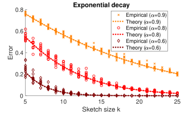
(a) Singular values are given by $\sigma_{i}^{2}=C\cdot\alpha^{i-1}$.

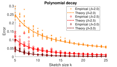
(b) Singular values are given by $\sigma_{i}^{2}=C\cdot i^{-\beta}$.

Figure 1: Theoretical predictions of low-rank approximation error of a Gaussian sketch under known spectral decays, compared to the empirical results. The constant $C$ is scaled so that $\|\mathbf{A}\|_{F}^{2}=1$ and we let $n=m=1000$. For the theory, we plot the explicit formulas (5) and (6) (dashed lines), as well as the implicit expression from Corollary 1 (thin solid lines) obtained by numerically solving (4). Observe that the explicit and implicit predictions are nearly (but not exactly) identical.

3.1 Exponential spectral decay

Suppose that the squared singular values of $\mathbf{A}$ exhibit exponential decay, i.e. $\sigma_{i}^{2}=C\cdot\alpha^{i-1}$, where $C$ is a constant and $\alpha\in(0,1)$. For simplicity of presentation, we will let $m,n\rightarrow\infty$. Under this spectral decay, we can approximate the sum in (4) by the analytically computable integral $\int_{y}^{\infty}\!\frac{1}{1+(C\gamma)^{-1}\alpha^{-x}}dx$, obtaining $\gamma\approx(\alpha^{-k}-1)\sqrt{\alpha}/C$. Applying this to the formula from Corollary 1, we can express the low-rank approximation error for a sketch of size $k$ as follows:

$$\mathbb{E}\big{[}\|\mathbf{A}-\mathbf{A}\mathbf{P}\|_{F}^{2}\big{]}\approx\frac{C}{\sqrt{\alpha}}\cdot\frac{k}{\alpha^{-k}-1},\quad\text{when}\quad\sigma_{i}^{2}=C\cdot\alpha^{i-1}\ \ \text{for all $i$.}$$ (5)

In Figure 1a, we plot the above formula against the numerically obtained implicit expression from Corollary 1, as well as empirical results for a Gaussian sketch. First, we observe that the theoretical predictions closely align with empirical values even after the sketch size crosses the stable rank $r\approx\frac{1}{1-\alpha}$, suggesting that Theorem 1 can be extended to this regime. Second, while it is not surprising that the error decays at a similar rate as the singular values, our predictions offer a much more precise description, down to lower order effects and even constant factors. For instance, we observe that the error (normalized by $\|\mathbf{A}\|_{F}^{2}$, as in the figure) only starts decaying exponentially after $k$ crosses the stable rank, and until that point it decreases at a linear rate with slope $-\frac{1-\alpha}{2\sqrt{\alpha}}$.

3.2 Polynomial spectral decay

We now turn to polynomial spectral decay, which is a natural model for analyzing heavy-tailed data distributions. Let $\mathbf{A}$ have squared singular values $\sigma_{i}^{2}=C\cdot i^{-\beta}$ for some $\beta\geq 2$, and let $m,n\rightarrow\infty$. As in the case of exponential decay, we use the integral $\int_{y}^{\infty}\!\frac{1}{1+(C\gamma)^{-1}x^{-\beta}}dx$ to approximate the sum in (4), and solve for $\gamma$, obtaining $\gamma\approx\big{(}(k+\frac{1}{2})\frac{\beta}{\pi}\sin(\frac{\pi}{\beta})\big{)}^{\beta}$. Combining this with Corollary 1 we get:

$$\mathbb{E}\big{[}\|\mathbf{A}-\mathbf{A}\mathbf{P}\|_{F}^{2}\big{]}\approx C\cdot\frac{k}{(k+\frac{1}{2})^{\beta}}\bigg{(}\frac{\pi/\beta}{\sin(\pi/\beta)}\bigg{)}^{\beta},\quad\text{when}\quad\sigma_{i}^{2}=C\cdot i^{-\beta}\ \ \text{for all $i$.}$$ (6)

Figure 1b compares our predictions to the empirical results for several values of $\beta$. In all of these cases, the stable rank is close to 1, and yet the theoretical predictions align very well with the empirical results. Overall, the asymptotic rate of decay of the error is $k^{1-\beta}$. However it is easy to verify that the lower order effect of $(k+\frac{1}{2})^{\beta}$ appearing instead of $k^{\beta}$ in (6) significantly changes the trajectory for small values of $k$. Also, note that as $\beta$ grows large, the constant $\big{(}\frac{\pi/\beta}{\sin(\pi/\beta)}\big{)}^{\beta}$ goes to $1$, but it plays a significant role for $\beta=2$ or $3$ (roughly, scaling the expression by a factor of $2$). Finally, we remark that for $\beta\in(1,2)$, our integral approximation of (4) becomes less accurate. We expect that a corrected expression is possible, but likely more complicated and less interpretable.

4 Empirical results

In this section, we numerically verify the accuracy of our theoretical predictions for the low-rank approximation error of sketching on benchmark datasets from the libsvm repository [CL11] (further numerical results are in Appendix C). We repeated every experiment 10 times, and plot both the average and standard deviation of the results. We use the following $k\times m$ sketching matrices $\mathbf{S}$:

1. Gaussian sketch: with i.i.d. standard normal entries;

2. Rademacher sketch: with i.i.d. entries equal $1$ with probability 0.5 and $-1$ otherwise.

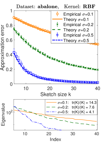
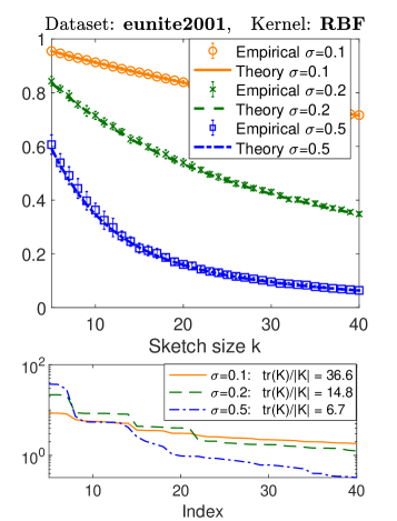
Figure 2: Theoretical predictions versus approximation error for the sketched Nyström with the RBF kernel (spectral decay shown at the bottom).

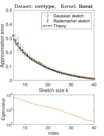
Figure 3: Theoretical predictions versus approximation error for the Gaussian and Rademacher sketches (spectral decay shown at the bottom).

Varying spectral decay.

To demonstrate the role of spectral decay and the stable rank on the approximation error, we performed feature expansion using the radial basis function (RBF) kernel $k(\mathbf{a}_{i},\mathbf{a}_{j})=\exp(-\|\mathbf{a}_{i}-\mathbf{a}_{j}\|^{2}/(2\sigma^{2}))$, obtaining an $m\times m$ kernel matrix $\mathbf{K}$. We used the sketched Nyström method to construct a low-rank approximation $\tilde{\mathbf{K}}=\mathbf{K}\mathbf{S}^{\scriptscriptstyle{\top}}(\mathbf{S}\mathbf{K}\mathbf{S}^{\scriptscriptstyle{\top}})^{\dagger}\mathbf{S}\mathbf{K}$, and computed the normalized trace norm error $\|\mathbf{K}-\tilde{\mathbf{K}}\|_{*}/\|\mathbf{K}\|_{*}$. The theoretical predictions are coming from (2), which in turn uses Theorem 1. Following [GM16], we use the RBF kernel because varying the scale parameter $\sigma$ allows us to observe the approximation error under qualitatively different spectral decay profiles of the kernel. In Figure 2, we present the results for the Gaussian sketch on two datasets, with three values of $\sigma$, and in all cases our theory aligns with the empirical results. Furthermore, as smaller $\sigma$ leads to slower spectral decay and larger stable rank, it also makes the approximation error decay more linearly for small sketch sizes. This behavior is predicted by our explicit expressions (5) for the error under exponential spectral decay from Section 3. Once the sketch sizes are sufficiently larger than the stable rank of $\mathbf{K}^{\frac{1}{2}}$, the error starts decaying at an exponential rate. Note that Theorem 1 only guarantees accuracy of our expressions for sketch sizes below the stable rank, however the predictions are accurate regardless of this constraint.

Varying sketch type.

In the next set of empirical results, we compare the performance of Gaussian and Rademacher sketches, and also verify the theory when sketching the data matrix $\mathbf{A}$ without kernel expansion, plotting $\|\mathbf{A}-\mathbf{A}(\mathbf{S}\mathbf{A})^{\dagger}\mathbf{S}\mathbf{A}\|_{F}^{2}/\|\mathbf{A}\|_{F}^{2}$. Since both of the sketching methods have sub-gaussian entries, Corollary 1 predicts that they should have comparable performance in this task and match our expressions. This is exactly what we observe in Figure 3 for two datasets and a range of sketching sizes, as well as in other empirical results shown in Appendix C.

5 Conclusions

We derived the first theoretically supported precise expressions for the expected residual projection matrix, which is a central component in the analysis of RandNLA dimensionality reduction via sketching. Our analysis provides a new understanding of low-rank approximation, the Nyström method, and the convergence properties of many randomized iterative algorithms. As a direction for future work, we conjecture that our main result can be extended to sketch sizes larger than the stable rank of the data matrix.

Acknowledgments.

We would like to acknowledge DARPA, IARPA, NSF, and ONR via its BRC on RandNLA for providing partial support of this work. Our conclusions do not necessarily reflect the position or the policy of our sponsors, and no official endorsement should be inferred.

Appendix A Proof of Theorem 2

We first introduce the following technical lemmas.

Lemma 1.

For $\mathbf{X}\in\mathbb{R}^{k\times n}$ with $k<n$, denote $\mathbf{P}=\mathbf{X}^{\dagger}\mathbf{X}$ and $\mathbf{P}_{-k}=\mathbf{X}_{-k}^{\dagger}\mathbf{X}_{-k}$, with $\mathbf{X}_{-i}\in\mathbb{R}^{(k-1)\times n}$ the matrix $\mathbf{X}$ without its i-th row $\mathbf{x}_{i}\in\mathbb{R}^{n}$. Then, conditioned on the event $E_{k}:\left\{\left|\frac{\mathrm{tr}\mathbf{\Sigma}(\mathbf{I}-\mathbf{P}_{-k})}{\mathbf{x}_{k}^{\scriptscriptstyle{\top}}(\mathbf{I}-\mathbf{P}_{-k})\mathbf{x}_{k}}-1\right|\leq\frac{1}{2}\right\}$:

$$(\mathbf{X}^{\scriptscriptstyle{\top}}\mathbf{X})^{\dagger}\mathbf{x}_{k}=\frac{(\mathbf{I}-\mathbf{P}_{-k})\mathbf{x}_{k}}{\mathbf{x}_{k}^{\scriptscriptstyle{\top}}(\mathbf{I}-\mathbf{P}_{-k})\mathbf{x}_{k}},\quad\mathbf{P}-\mathbf{P}_{-k}=\frac{(\mathbf{I}-\mathbf{P}_{-k})\mathbf{x}_{k}\mathbf{x}_{k}^{\scriptscriptstyle{\top}}(\mathbf{I}-\mathbf{P}_{-k})}{\mathbf{x}_{k}^{\scriptscriptstyle{\top}}(\mathbf{I}-\mathbf{P}_{-k})\mathbf{x}_{k}}.$$

Proof.

Since conditioned on $E_{k}$ we have $\mathbf{x}_{k}^{\scriptscriptstyle{\top}}(\mathbf{I}-\mathbf{P}_{-k})\mathbf{x}_{k}\neq 0$, from [Mey73, Theorem 1] we deduce

$$(\mathbf{X}^{\scriptscriptstyle{\top}}\mathbf{X})^{\dagger}=\left(\mathbf{A}+\mathbf{x}_{k}\mathbf{x}_{k}^{\scriptscriptstyle{\top}}\right)^{\dagger} =\mathbf{A}^{\dagger}-\frac{\mathbf{A}^{\dagger}\mathbf{x}_{k}\mathbf{x}_{k}^{\scriptscriptstyle{\top}}(\mathbf{I}-\mathbf{P}_{-k})}{\mathbf{x}_{k}^{\scriptscriptstyle{\top}}(\mathbf{I}-\mathbf{P}_{-k})\mathbf{x}_{k}}-\frac{(\mathbf{I}-\mathbf{P}_{-k})\mathbf{x}_{k}\mathbf{x}_{k}^{\scriptscriptstyle{\top}}\mathbf{A}^{\dagger}}{\mathbf{x}_{k}^{\scriptscriptstyle{\top}}(\mathbf{I}-\mathbf{P}_{-k})\mathbf{x}_{k}}$$

$$+(1+\mathbf{x}_{k}^{\scriptscriptstyle{\top}}\mathbf{A}^{\dagger}\mathbf{x}_{k})\frac{(\mathbf{I}-\mathbf{P}_{-k})\mathbf{x}_{k}\mathbf{x}_{k}^{\scriptscriptstyle{\top}}(\mathbf{I}-\mathbf{P}_{-k})}{(\mathbf{x}_{k}^{\scriptscriptstyle{\top}}(\mathbf{I}-\mathbf{P}_{-k})\mathbf{x}_{k})^{2}}$$

for $\mathbf{A}=\mathbf{X}_{-k}^{\scriptscriptstyle{\top}}\mathbf{X}_{-k}$ so that $\mathbf{I}-\mathbf{P}_{-k}=\mathbf{I}-\mathbf{A}^{\dagger}\mathbf{A}$, where we used the fact that $\mathbf{I}-\mathbf{P}_{-k}$ is a projection matrix so that $(\mathbf{I}-\mathbf{P}_{-k})^{2}=\mathbf{I}-\mathbf{P}_{-k}$. As a consequence, multiplying by $\mathbf{x}_{k}$ and simplifying we get

$$(\mathbf{X}^{\scriptscriptstyle{\top}}\mathbf{X})^{\dagger}\mathbf{x}_{k}=\frac{(\mathbf{I}-\mathbf{P}_{-k})\mathbf{x}_{k}}{\mathbf{x}_{k}^{\scriptscriptstyle{\top}}(\mathbf{I}-\mathbf{P}_{-k})\mathbf{x}_{k}}.$$

By definition of the pseudoinverse, $\mathbf{P}=\mathbf{X}^{\dagger}\mathbf{X}=(\mathbf{X}^{\scriptscriptstyle{\top}}\mathbf{X})^{\dagger}\mathbf{X}^{\scriptscriptstyle{\top}}\mathbf{X}$ so that

$$\mathbf{P}-\mathbf{P}_{-k}=\mathbf{X}^{\dagger}\mathbf{X}-\mathbf{X}_{-k}^{\dagger}\mathbf{X}_{-k}=\frac{(\mathbf{I}-\mathbf{P}_{-k})\mathbf{x}_{k}\mathbf{x}_{k}^{\scriptscriptstyle{\top}}(\mathbf{I}-\mathbf{P}_{-k})}{\mathbf{x}_{k}^{\scriptscriptstyle{\top}}(\mathbf{I}-\mathbf{P}_{-k})\mathbf{x}_{k}}$$

where we used $\mathbf{A}(\mathbf{I}-\mathbf{P}_{-k})=\mathbf{A}-\mathbf{A}\mathbf{A}^{\dagger}\mathbf{A}=0$ and thus the conclusion. ∎

Lemma 2.

If random vector $\mathbf{x}\in\mathbb{R}^{n}$, with $\mathbb{E}[\mathbf{x}]=0$ and $\mathbb{E}[\mathbf{x}\mathbf{x}^{\scriptscriptstyle{\top}}]=\mathbf{I}_{n}$, satisfies the Hanson-Wright inequality with constant $K\geq 1$ (Definition 1), then for any positive semi-definite matrix $\mathbf{A}\in\mathbb{R}^{n\times n}$, we have

$$\mathrm{Pr}\left[\lvert\mathbf{x}^{\scriptscriptstyle{\top}}\mathbf{A}\mathbf{x}-\mathrm{tr}\mathbf{A}\rvert\geq\frac{1}{3}\mathrm{tr}\mathbf{A}\right]\leq 2\exp\left(-\frac{r_{\!\mathbf{A}}}{CK^{4}}\right)$$

with $r_{\!\mathbf{A}}=\mathrm{tr}\mathbf{A}/\|\mathbf{A}\|$ the stable rank of $\mathbf{A}$, and

$$\mathbb{E}\left[\left(\mathbf{x}^{\scriptscriptstyle{\top}}\mathbf{A}\mathbf{x}-\mathrm{tr}\mathbf{A}\right)^{2}\right] \leq c~{}K^{4}~{}\mathrm{tr}\mathbf{A}^{2}$$

for some $C,c>0$ independent of $K$. Also, for any unit vector $\mathbf{v}\in\mathbb{R}^{n}$, variable $\mathbf{v}^{\scriptscriptstyle{\top}}\mathbf{x}$ is $CK$-sub-gaussian.

Proof.

Recall that, for a psd matrix $\mathbf{A}$, the Hanson-Wright inequality can be stated as follows:

$$\mathrm{Pr}\left\{\left|\mathbf{x}^{\scriptscriptstyle{\top}}\mathbf{A}\mathbf{x}-\mathrm{tr}\mathbf{A}\right|\geq t\right\}\leq 2\exp\left(-\min\left\{\frac{t^{2}}{K^{4}\mathrm{tr}\mathbf{A}^{2}},\frac{t}{K^{2}\|\mathbf{A}\|}\right\}\right).$$

Taking $t=\frac{1}{3}\mathrm{tr}\mathbf{A}$ we have

$$\frac{t^{2}}{K^{4}\mathrm{tr}\mathbf{A}^{2}}=\frac{(\mathrm{tr}\mathbf{A})^{2}}{9K^{4}\mathrm{tr}\mathbf{A}^{2}}\geq\frac{\mathrm{tr}\mathbf{A}}{9K^{4}\|\mathbf{A}\|}=\frac{r_{\!\mathbf{A}}}{9K^{4}},\qquad\frac{t}{K^{2}\|\mathbf{A}\|}\geq\frac{r_{\!\mathbf{A}}}{3K^{2}},$$

where we use the fact that $\mathrm{tr}\mathbf{A}^{2}\leq\|\mathbf{A}\|\mathrm{tr}\mathbf{A}$.

Integrating this bound yields:

$$\mathbb{E}\left[(\mathbf{x}^{\scriptscriptstyle{\top}}\mathbf{A}\mathbf{x}-\mathrm{tr}\mathbf{A})^{2}\right]\leq c~{}K^{4}~{}\mathrm{tr}\mathbf{A}^{2}.$$

Finally, to obtain the sub-gaussianity of $\mathbf{v}^{\scriptscriptstyle{\top}}\mathbf{x}$, we apply the Hanson-Wright inequality to $\mathbf{A}=\mathbf{v}\mathbf{v}^{\scriptscriptstyle{\top}}$. ∎

Lemma 3.

With the notations of Lemma 1, for $X=\mathrm{tr}\,\mathbf{\Sigma}(\mathbf{P}_{-k}-\mathbb{E}[\mathbf{P}_{-k}])$ and $\|\mathbf{\Sigma}\|=1$, we have

$$\mathbb{E}[X^{2}]\leq Ck\quad\text{and}\quad\mathrm{Pr}\{|X|\geq t\}\leq 2\mathrm{e}^{-\frac{t^{2}}{ck}}.$$

for some universal constant $C,c>0$.

Proof.

To simplify notations, we work on $\mathbf{P}$ instead of $\mathbf{P}_{-k}$, the same line of argument applies to $\mathbf{P}_{-k}$ by changing the sample size $k$ to $k-1$.

First note that

$$X =\mathrm{tr}\mathbf{\Sigma}(\mathbf{P}-\mathbb{E}\mathbf{P})=\mathbb{E}_{k}[\mathrm{tr}\mathbf{\Sigma}\mathbf{P}]-\mathbb{E}_{0}[\mathrm{tr}\mathbf{\Sigma}\mathbf{P}]$$

$$=\sum_{i=1}^{k}\left(\mathbb{E}_{i}[\mathrm{tr}\mathbf{\Sigma}\mathbf{P}]-\mathbb{E}_{i-1}[\mathrm{tr}\mathbf{\Sigma}\mathbf{P}]\right)=\sum_{i=1}^{k}(\mathbb{E}_{i}-\mathbb{E}_{i-1})\mathrm{tr}\mathbf{\Sigma}(\mathbf{P}-\mathbf{P}_{-i})$$

where we used the fact that $\mathbb{E}_{i}[\mathrm{tr}\mathbf{\Sigma}\mathbf{P}_{-i}]=\mathbb{E}_{i-1}[\mathrm{tr}\mathbf{\Sigma}\mathbf{P}_{-i}]$, for $\mathbb{E}_{i}[\cdot]$ the conditional expectation with respect to $\mathcal{F}_{i}$ the $\sigma$-field generating the rows $\mathbf{x}_{1}\ldots,\mathbf{x}_{i}$ of $\mathbf{X}$. This forms a martingale difference sequence (it is a difference sequence of the Doob martingale for $\mathrm{tr}\mathbf{\Sigma}(\mathbf{P}-\mathbf{P}_{-i})$ with respect to filtration $\mathcal{F}_{i}$) hence it falls within the scope of the Burkholder inequality [Bur73], recalled as follows.

Lemma 4.

For $\{x_{i}\}_{i=1}^{k}$ a real martingale difference sequence with respect to the increasing $\sigma$ field $\mathcal{F}_{i}$, we have, for $L>1$, there exists $C_{L}>0$ such that

$$\mathbb{E}\bigg{[}\Big{|}\sum_{i=1}^{k}x_{i}\Big{|}^{L}\bigg{]}\leq C_{L}\mathbb{E}\bigg{[}\Big{(}\sum_{i=1}^{k}|x_{i}|^{2}\Big{)}^{L/2}\bigg{]}.$$

From Lemma 1, $\mathbf{P}-\mathbf{P}_{-i}=\frac{(\mathbf{I}-\mathbf{P}_{-i})\mathbf{x}_{i}\mathbf{x}_{i}^{\scriptscriptstyle{\top}}(\mathbf{I}-\mathbf{P}_{-i})}{\mathbf{x}_{i}^{\scriptscriptstyle{\top}}(\mathbf{I}-\mathbf{P}_{-i})\mathbf{x}_{i}}$ is positive semi-definite, we have $\mathrm{tr}\mathbf{\Sigma}(\mathbf{P}-\mathbf{P}_{-i})\leq\|\mathbf{\Sigma}\|=1$ so that with Lemma 4 we obtain with $x_{i}=(\mathbb{E}_{i}-\mathbb{E}_{i-1})\mathrm{tr}\mathbf{\Sigma}(\mathbf{P}-\mathbf{P}_{-i})$ that, for $L>1$

$$\mathbb{E}|X|^{L}\leq C_{L}k^{L/2}.$$

In particular, for $L=2$, we obtain $\mathbb{E}|X|^{2}\leq Ck$.

For the second result, since we have almost surely bounded martingale differences ($\lvert x_{i}\rvert\leq 2$), by the Azuma-Hoeffding inequality

$$\mathrm{Pr}\{\lvert X\rvert\geq t\}\leq 2\mathrm{e}^{\frac{-t^{2}}{8k}}$$

as desired. ∎

A.1 Complete proof of Theorem 2

Equipped with the lemmas above, we are ready to prove Theorem 2. First note that:

1. Since $\mathbf{X}^{\dagger}\mathbf{X}\overset{d}{=}(\alpha\mathbf{X})^{\dagger}(\alpha\mathbf{X})$ for any $\alpha\in\mathbb{R}\setminus\{0\}$, we can assume without loss of generality (after rescaling $\bar{\mathbf{P}}_{\perp}$ correspondingly) that $\|\mathbf{\Sigma}\|=1$.

2. According to the definition of $\bar{\mathbf{P}}_{\perp}$ and $\gamma$, the following bounds hold

   $$\frac{1}{\gamma+1}\mathbf{I}\preceq\bar{\mathbf{P}}_{\perp}\preceq\mathbf{I},\quad\gamma\leq\frac{k}{r-k}=\frac{1}{\rho-1}$$ (7)

   for $r\equiv\frac{\mathrm{tr}\mathbf{\Sigma}}{\|\mathbf{\Sigma}\|}=\mathrm{tr}\mathbf{\Sigma}$ and $\rho\equiv\frac{r}{k}>1$, where we used the fact that

   $$k=n-\mathrm{tr}\,\bar{\mathbf{P}}_{\perp}=\mathrm{tr}\,\bar{\mathbf{P}}_{\perp}(\gamma\mathbf{\Sigma}+\mathbf{I})-\mathrm{tr}\,\bar{\mathbf{P}}_{\perp}=\gamma\mathrm{tr}\,\bar{\mathbf{P}}_{\perp}\mathbf{\Sigma}\geq\frac{\gamma}{\gamma+1}\mathrm{tr}\,\mathbf{\Sigma},$$

   so that $r=\mathrm{tr}\mathbf{\Sigma}\leq k\cdot\frac{\gamma+1}{\gamma}$.

3. As already discussed in Section 2.1, to obtain the lower and upper bound for $\mathbb{E}[\mathbf{P}_{\perp}]$ in the sense of symmetric matrix as in Theorem 2, it suffices to bound the following spectral norm

   $$\|\mathbf{I}-\mathbb{E}[\mathbf{P}_{\perp}]\bar{\mathbf{P}}_{\perp}^{-1}\|\leq\frac{C_{\rho}}{\sqrt{r}},$$ (8)

   so that, with $\frac{\rho-1}{\rho}\mathbf{I}\preceq\bar{\mathbf{P}}_{\perp}\preceq\mathbf{I}$ from (7), we have

   $$\|\mathbf{I}-\bar{\mathbf{P}}_{\perp}^{-\frac{1}{2}}\mathbb{E}[\mathbf{P}_{\perp}]\bar{\mathbf{P}}_{\perp}^{-\frac{1}{2}}\|=\|\bar{\mathbf{P}}_{\perp}^{-\frac{1}{2}}(\mathbf{I}-\mathbb{E}[\mathbf{P}_{\perp}]\bar{\mathbf{P}}_{\perp}^{-1})\bar{\mathbf{P}}_{\perp}^{\frac{1}{2}}\|\leq\frac{C_{\rho}}{\sqrt{r}}\sqrt{\frac{\rho}{\rho-1}}.$$

   Defining $\epsilon=\frac{C_{\rho}}{\sqrt{r}}\sqrt{\frac{\rho}{\rho-1}}$, this means that all eigenvalues of the p.s.d. matrix $\bar{\mathbf{P}}_{\perp}^{-\frac{1}{2}}\mathbb{E}[\mathbf{P}_{\perp}]\bar{\mathbf{P}}_{\perp}^{-\frac{1}{2}}$ lie in the interval $[1-\epsilon,1+\epsilon]$, and

   $$(1-\epsilon)\mathbf{I}\preceq\bar{\mathbf{P}}_{\perp}^{-\frac{1}{2}}\mathbb{E}[\mathbf{P}_{\perp}]\bar{\mathbf{P}}_{\perp}^{-\frac{1}{2}}\preceq(1+\epsilon)\mathbf{I}.$$

   so that by multiplying $\bar{\mathbf{P}}_{\perp}^{\frac{1}{2}}$ on both sides, we obtain the desired bound.

As a consequence of the above observations, we only need to prove (8) under the setting $\|\mathbf{\Sigma}\|=1$. The proof comes in the following two steps:

1. For $\mathbf{P}_{-i}=\mathbf{X}_{-i}^{\dagger}\mathbf{X}_{-i}$, with $\mathbf{X}_{-i}\in\mathbb{R}^{(k-1)\times n}$ the matrix $\mathbf{X}$ without its $i$-th row, we define, for $i\in\{1,\ldots,k\}$, the following events

   $$E_{i}:\left\{\left|\frac{\mathrm{tr}(\mathbf{I}-\mathbf{P}_{-i})\mathbf{\Sigma}}{\mathbf{x}_{i}^{\scriptscriptstyle{\top}}(\mathbf{I}-\mathbf{P}_{-i})\mathbf{x}_{i}}-1\right|\leq\frac{1}{2}\right\},$$ (9)

   where we recall $\mathbf{x}_{i}\in\mathbb{R}^{n}$ is the $i$-th row of $\mathbf{X}$ so that $\mathbb{E}[\mathbf{x}_{i}]=0$ and $\mathbb{E}[\mathbf{x}_{i}\mathbf{x}_{i}^{\scriptscriptstyle{\top}}]=\mathbf{\Sigma}$. With Lemma 2, we can bound the probability of $\neg E_{i}$, and consequently that of $\neg E$ for $E=\bigwedge_{i=1}^{k}E_{i}$;

2. We then bound, conditioned on $E$ and $\neg E$ respectively, the spectral norm $\|\mathbf{I}-\mathbb{E}[\mathbf{P}_{\perp}]\bar{\mathbf{P}}_{\perp}^{-1}\|$. More precisely, since

   $$\mathbf{I}-\mathbb{E}[\mathbf{P}_{\perp}]\bar{\mathbf{P}}_{\perp}^{-1}\! =\mathbb{E}[\mathbf{P}]-\gamma\mathbb{E}[\mathbf{P}_{\perp}]\mathbf{\Sigma}=\mathbb{E}[\mathbf{P}\cdot\mathbf{1}_{E}]+\mathbb{E}[\mathbf{P}\cdot\mathbf{1}_{\neg E}]-\gamma\mathbb{E}[\mathbf{P}_{\perp}]\mathbf{\Sigma}$$

   $$=k\,\mathbb{E}\bigg{[}\frac{(\mathbf{I}-\mathbf{P}_{-k})\mathbf{x}_{k}\mathbf{x}_{k}^{\scriptscriptstyle{\top}}}{\mathbf{x}_{k}^{\scriptscriptstyle{\top}}(\mathbf{I}-\mathbf{P}_{-k})\mathbf{x}_{k}}\cdot\mathbf{1}_{E}\bigg{]}-\gamma\mathbb{E}[\mathbf{P}_{\perp}]\mathbf{\Sigma}\ +\ \mathbb{E}[\mathbf{P}\cdot\mathbf{1}_{\neg E}]$$

   $$=\gamma\underbrace{\mathbb{E}\bigg{[}(\bar{s}-\hat{s})\,\frac{(\mathbf{I}-\mathbf{P}_{-k})\mathbf{x}_{k}\mathbf{x}_{k}^{\scriptscriptstyle{\top}}}{\mathbf{x}_{k}^{\scriptscriptstyle{\top}}(\mathbf{I}-\mathbf{P}_{-k})\mathbf{x}_{k}}\cdot\mathbf{1}_{E}\bigg{]}}_{\mathbf{T}_{1}}-\gamma\underbrace{\mathbb{E}[(\mathbf{I}-\mathbf{P}_{-k})\mathbf{x}_{k}\mathbf{x}_{k}^{\scriptscriptstyle{\top}}\cdot\mathbf{1}_{\neg E}]}_{\mathbf{T}_{2}}+\gamma\underbrace{\mathbb{E}[\mathbf{P}-\mathbf{P}_{-k}]\mathbf{\Sigma}}_{\mathbf{T}_{3}}+\underbrace{\mathbb{E}[\mathbf{P}\cdot\mathbf{1}_{\neg E}]}_{\mathbf{T}_{4}},$$

   where we used Lemma 1 for the third equality and denote $\hat{s}=\mathbf{x}_{k}^{\scriptscriptstyle{\top}}(\mathbf{I}-\mathbf{P}_{-k})\mathbf{x}_{k}$ as well as $\bar{s}=\mathrm{tr}\bar{\mathbf{P}}_{\perp}\mathbf{\Sigma}=k/\gamma$. It then remains to bound the spectral norms of $\mathbf{T}_{1},\mathbf{T}_{2},\mathbf{T}_{3},\mathbf{T}_{4}$ to reach the conclusion.

Another important relation that will be constantly used throughout the proof is

$$\mathrm{tr}(\mathbf{I}-\mathbf{P}_{-k})\mathbf{\Sigma}=\mathrm{tr}\mathbf{\Sigma}^{\frac{1}{2}}(\mathbf{I}-\mathbf{P}_{-k})^{2}\mathbf{\Sigma}^{\frac{1}{2}}=\|\mathbf{\Sigma}^{\frac{1}{2}}-\mathbf{\Sigma}^{\frac{1}{2}}\mathbf{X}_{-k}^{\dagger}\mathbf{X}_{-k}\|_{F}^{2}\geq\sum_{i\geq k}\lambda_{i}(\mathbf{\Sigma})\geq r-k$$ (10)

where we used the fact that $\mathrm{rank}(\mathbf{X}_{-k}^{\dagger}\mathbf{X}_{-k})\leq\mathrm{rank}(\mathbf{X}_{-k})\leq k-1$ and arranged the eigenvalues $1=\lambda_{1}(\mathbf{\Sigma})\geq\ldots\geq\lambda_{n}(\mathbf{\Sigma})$ in a non-increasing order. As a consequence, we also have

$$\frac{\mathrm{tr}(\mathbf{I}-\mathbf{P}_{-k})\mathbf{\Sigma}}{\|\mathbf{\Sigma}^{\frac{1}{2}}(\mathbf{I}-\mathbf{P}_{-k})\mathbf{\Sigma}^{\frac{1}{2}}\|}\geq\mathrm{tr}(\mathbf{I}-\mathbf{P}_{-k})\mathbf{\Sigma}\geq r-k.$$ (11)

For the first step, assuming without loss of generality that that the Hanson-Wright constant satisfies $K\geq 1$ and using Lemma 2 together with (11), we have:

$$\mathrm{Pr}(\neg E_{i}) \leq\mathrm{Pr}\left\{\lvert\mathbf{x}_{i}^{\scriptscriptstyle{\top}}(\mathbf{I}-\mathbf{P}_{-i})\mathbf{x}_{i}-\mathrm{tr}\mathbf{\Sigma}(\mathbf{I}-\mathbf{P}_{-i})\rvert\geq\frac{1}{3}\mathrm{tr}\mathbf{\Sigma}(\mathbf{I}-\mathbf{P}_{-i})\right\}\leq 2\mathrm{e}^{-\frac{r-k}{CK^{4}}},$$

so that with the union bound we obtain

$$\mathrm{Pr}(\neg E)\leq 2k\mathrm{e}^{-\frac{r-k}{CK^{4}}}\leq\frac{k}{(r-k)^{2}}\cdot 2(r-k)^{2}\mathrm{e}^{-\frac{r-k}{CK^{4}}}\leq\frac{C_{\rho}}{r-k},$$ (12)

where we used the fact that, for $\alpha,x>0$, we have $x^{2}\mathrm{e}^{-\alpha x}\leq\frac{4\mathrm{e}^{-2}}{\alpha^{2}}$. Also, denoting $c_{\rho}=\frac{r-k}{r}=\frac{\rho-1}{\rho}>0$, we have

$$\mathrm{Pr}(\neg E)\leq\frac{C_{\rho}}{r-k}=\frac{C_{\rho}}{c_{\rho}r}=\frac{C^{\prime}_{\rho}}{r}$$ (13)

for some $C^{\prime}_{\rho}>0$ that depends on $\rho=r/k>1$ and the Hanson-Wright constant $K$.

At this point, note that, conditioned on the event $E$, we have for $i\in\{1,\ldots,k\}$

$$\frac{1}{2}\frac{1}{\mathrm{tr}(\mathbf{I}-\mathbf{P}_{-i})\mathbf{\Sigma}}\leq\frac{1}{\mathbf{x}_{i}^{\scriptscriptstyle{\top}}(\mathbf{I}-\mathbf{P}_{-i})\mathbf{x}_{i}}\leq\frac{3}{2}\frac{1}{\mathrm{tr}(\mathbf{I}-\mathbf{P}_{-i})\mathbf{\Sigma}},$$ (14)

Also, with (13) and the fact that $\|\mathbf{P}\|\leq 1$, we have $\|\mathbf{T}_{4}\|\leq\frac{C_{\rho}}{r}$ for some $C_{\rho}>0$ that depends on $\rho$ and $K$. To handle non-symmetric matrix $\mathbf{T}_{2}$, note that $\mathbf{T}_{2}+\mathbf{T}_{2}^{\scriptscriptstyle{\top}}$ is symmetric and

$$-\mathbb{E}[(\mathbf{I}-\mathbf{P}_{-k})\cdot\mathbf{1}_{\neg E}]-\mathbb{E}[(\mathbf{x}_{k}^{\scriptscriptstyle{\top}}\mathbf{x}_{k})\mathbf{x}_{k}\mathbf{x}_{k}^{\scriptscriptstyle{\top}}\cdot\mathbf{1}_{\neg E}]\preceq\mathbf{T}_{2}+\mathbf{T}_{2}^{\scriptscriptstyle{\top}}\preceq\mathbb{E}[(\mathbf{I}-\mathbf{P}_{-k})\cdot\mathbf{1}_{\neg E}]+\mathbb{E}[(\mathbf{x}_{k}^{\scriptscriptstyle{\top}}\mathbf{x}_{k})\mathbf{x}_{k}\mathbf{x}_{k}^{\scriptscriptstyle{\top}}\cdot\mathbf{1}_{\neg E}]$$ (15)

with $-(\mathbf{A}\mathbf{A}^{\scriptscriptstyle{\top}}+\mathbf{B}\mathbf{B}^{\scriptscriptstyle{\top}})\preceq\mathbf{A}\mathbf{B}^{\scriptscriptstyle{\top}}+\mathbf{B}\mathbf{A}^{\scriptscriptstyle{\top}}\preceq\mathbf{A}\mathbf{A}^{\scriptscriptstyle{\top}}+\mathbf{B}\mathbf{B}^{\scriptscriptstyle{\top}}$. To obtain an upper bound for operator norm of $\mathbb{E}[(\mathbf{x}_{k}^{\scriptscriptstyle{\top}}\mathbf{x}_{k})\mathbf{x}_{k}\mathbf{x}_{k}^{\scriptscriptstyle{\top}}\cdot\mathbf{1}_{\neg E}]$, note that

$$\|\mathbb{E}[(\mathbf{x}_{k}^{\scriptscriptstyle{\top}}\mathbf{x}_{k})\mathbf{x}_{k}\mathbf{x}_{k}^{\scriptscriptstyle{\top}}\cdot\mathbf{1}_{\neg E}]\| \leq\mathbb{E}[(\mathbf{x}_{k}^{\scriptscriptstyle{\top}}\mathbf{x}_{k})^{2}\cdot\mathbf{1}_{\neg E}]=\int_{0}^{\infty}\mathrm{Pr}(\mathbf{x}^{\scriptscriptstyle{\top}}\mathbf{x}\cdot\mathbf{1}_{\neg E}\geq\sqrt{t})dt$$

$$\leq\int_{0}^{X}\mathrm{Pr}(\mathbf{x}^{\scriptscriptstyle{\top}}\mathbf{x}\cdot\mathbf{1}_{\neg E}\geq\sqrt{t})dt+\int_{X}^{\infty}\mathrm{Pr}(\mathbf{x}^{\scriptscriptstyle{\top}}\mathbf{x}\geq\sqrt{t})dt$$

$$\leq X\cdot\mathrm{Pr}(\neg E)+\int_{X}^{\infty}\mathrm{e}^{-\min\left\{\frac{t}{C^{2}K^{4}r},\frac{\sqrt{t}}{CK^{2}\sqrt{r}}\right\}}dt\leq\frac{c_{\rho}}{r}$$

where we recall $\mathbb{E}[\mathbf{x}^{\scriptscriptstyle{\top}}\mathbf{x}]=\mathrm{tr}\mathbf{\Sigma}=r$ and take $X\geq C^{2}K^{4}r$, the third line follows from the proof of Lemma 2 and the forth line from the same argument as in (12). Moreover, since $\|\mathbf{T}_{2}\|\leq\|\mathbf{T}_{2}+\mathbf{T}_{2}^{\scriptscriptstyle{\top}}\|$ (see for example [Ser10, Proposition 5.11]), we conclude that $\|\mathbf{T}_{2}\|\leq\frac{C_{\rho}}{r}$.

And it thus remains to handle the terms $\mathbf{T}_{1}$ and $\mathbf{T}_{3}$ to obtain a bound on $\|\mathbf{I}-\mathbb{E}[\mathbf{P}_{\perp}]\bar{\mathbf{P}}_{\perp}^{-1}\|$.

To bound $\mathbf{T}_{3}$, with $\mathbf{P}-\mathbf{P}_{-k}=\frac{(\mathbf{I}-\mathbf{P}_{-k})\mathbf{x}_{k}\mathbf{x}_{k}^{\scriptscriptstyle{\top}}(\mathbf{I}-\mathbf{P}_{-k})}{\mathbf{x}_{k}^{\scriptscriptstyle{\top}}(\mathbf{I}-\mathbf{P}_{-k})\mathbf{x}_{k}}$ in Lemma 1, we have

$$\|\mathbf{T}_{3}\| \leq\bigg{\|}\mathbb{E}\bigg{[}\frac{(\mathbf{I}-\mathbf{P}_{-k})\mathbf{x}_{k}\mathbf{x}_{k}^{\scriptscriptstyle{\top}}(\mathbf{I}-\mathbf{P}_{-k})}{\mathbf{x}_{k}^{\scriptscriptstyle{\top}}(\mathbf{I}-\mathbf{P}_{-k})\mathbf{x}_{k}}\cdot\mathbf{1}_{E}\bigg{]}\bigg{\|}+\|\mathbb{E}[(\mathbf{P}-\mathbf{P}_{-k})\cdot\mathbf{1}_{\neg E}]\|$$

$$\leq\frac{3}{2}\mathbb{E}\left[\frac{1}{\mathrm{tr}(\mathbf{I}-\mathbf{P}_{-k})\mathbf{\Sigma}}\right]+\frac{c_{\rho}}{r-k}\leq\frac{C_{\rho}}{r-k}=\frac{C^{\prime}_{\rho}}{r}$$

where we used the fact that $\mathrm{tr}\,(\mathbf{I}-\mathbf{P}_{-k})\mathbf{\Sigma}\geq r-k$ from (10) and recall $\rho\equiv r/k>1$.

For $\mathbf{T}_{1}$ we write

$$\|\mathbf{T}_{1}\| \leq\mathbb{E}\bigg{[}\|\mathbf{I}-\mathbf{P}_{-k}\|\cdot\Big{\|}\mathbb{E}\Big{[}|\bar{s}-\hat{s}|\cdot\frac{\mathbf{x}_{k}\mathbf{x}_{k}^{\scriptscriptstyle{\top}}}{\mathbf{x}_{k}^{\scriptscriptstyle{\top}}(\mathbf{I}-\mathbf{P}_{-k})\mathbf{x}_{k}}\cdot\mathbf{1}_{E}\mid\mathbf{P}_{-k}\Big{]}\Big{\|}\bigg{]}$$

$$\leq\frac{3}{2}\frac{1}{r-k}\cdot\mathbb{E}\bigg{[}\sup_{\|\mathbf{v}\|=1}\mathbb{E}\Big{[}|\bar{s}-\hat{s}|\cdot\mathbf{v}^{\scriptscriptstyle{\top}}\mathbf{x}_{k}\mathbf{x}_{k}^{\scriptscriptstyle{\top}}\mathbf{v}\cdot\mathbf{1}_{E}\mid\mathbf{P}_{-k}\Big{]}\bigg{]}$$

$$\leq\frac{C_{\rho}}{r}\cdot\mathbb{E}\bigg{[}\underbrace{\sqrt{\mathbb{E}\big{[}(\bar{s}-\hat{s})^{2}\cdot\mathbf{1}_{E}\mid\mathbf{P}_{-k}\big{]}}}_{T_{1,1}}\cdot\underbrace{\sup_{\|\mathbf{v}\|=1}\sqrt{\mathbb{E}\big{[}(\mathbf{v}^{\scriptscriptstyle{\top}}\mathbf{x}_{k})^{4}\big{]}}}_{T_{1,2}}\bigg{]}$$

where we used Jensen’s inequality for the first inequality, the relation in (10) for the second inequality, and Cauchy–Schwarz for the third inequality.

We first bound $T_{1,2}$ by definition of sub-gaussian random vectors. From Lemma 2, for any unit vector $\mathbf{v}$, we have that $\mathbf{v}^{\scriptscriptstyle{\top}}\mathbf{x}_{k}$ is a $O(K)$-sub-gaussian random variable. As such, $T_{1,2}\leq CK^{2}$ for some absolute constant $C>0$, see for example [Ver18, Section 2.5.2].

For $T_{1,1}$ we have

$$\sqrt{\mathbb{E}\big{[}(\bar{s}-\hat{s})^{2}\cdot\mathbf{1}_{E}\mid\mathbf{P}_{-k}\big{]}}=\sqrt{(\bar{s}-s)^{2}+\mathbb{E}\big{[}(s-\hat{s})^{2}\cdot\mathbf{1}_{E}\big{]}}$$

where we denote $s=\mathbb{E}[\hat{s}]=\mathrm{tr}\,\mathbb{E}[\mathbf{I}-\mathbf{P}_{-k}]\mathbf{\Sigma}$. Note that

$$\mathbb{E}\big{[}(s-\hat{s})^{2}\big{]} =\mathbb{E}\big{[}\big{(}\mathrm{tr}\,\mathbf{\Sigma}(\mathbf{P}_{-k}-\mathbb{E}[\mathbf{P}_{-k}])\big{)}^{2}\big{]}+\mathbb{E}\big{[}(\mathrm{tr}\,(\mathbf{I}-\mathbf{P}_{-k})\mathbf{\Sigma}-\mathbf{x}_{k}^{\scriptscriptstyle{\top}}(\mathbf{I}-\mathbf{P}_{-k})\mathbf{x}_{k})^{2}\big{]}$$

$$\leq C_{1}k+C_{2}\mathbb{E}\big{[}\mathrm{tr}\,(\mathbf{\Sigma}-\mathbf{P}_{-k}\mathbf{\Sigma})^{2}\big{]}$$

$$\leq C(k+s)$$

$$\leq C\big{(}k+\bar{s}+|s-\bar{s}|\big{)}$$

where we used Lemma 3 and Lemma 2. Recall that $\bar{s}=\mathrm{tr}\bar{\mathbf{P}}_{\perp}\mathbf{\Sigma}\leq\mathrm{tr}\mathbf{\Sigma}=r$ and $k<r$, we have

$$T_{1,1}\leq\sqrt{(\bar{s}-s)^{2}+C\big{(}|\bar{s}-s|+2r\big{)}}.$$ (16)

It remains to bound $|\bar{s}-s|$. Note that $\mathbf{P}=(\mathbf{X}^{\scriptscriptstyle{\top}}\mathbf{X})^{\dagger}\mathbf{X}^{\scriptscriptstyle{\top}}\mathbf{X}=\mathbf{X}^{\scriptscriptstyle{\top}}\mathbf{X}(\mathbf{X}^{\scriptscriptstyle{\top}}\mathbf{X})^{\dagger}$ and is symmetric, so

$$\mathbf{I}-\mathbb{E}[\mathbf{P}_{\perp}]\bar{\mathbf{P}}_{\perp}^{-1}+\mathbf{I}-\bar{\mathbf{P}}_{\perp}^{-1}\mathbb{E}[\mathbf{P}_{\perp}]=2\mathbb{E}[\mathbf{P}]-\mathbb{E}[\gamma\mathbf{P}_{\perp}\mathbf{\Sigma}]-\mathbb{E}[\gamma\mathbf{\Sigma}\mathbf{P}_{\perp}]$$

$$=\sum_{i=1}^{k}\mathbb{E}\big{[}(\mathbf{X}^{\scriptscriptstyle{\top}}\mathbf{X})^{\dagger}\mathbf{x}_{i}\mathbf{x}_{i}^{\scriptscriptstyle{\top}}+\mathbf{x}_{i}\mathbf{x}_{i}^{\scriptscriptstyle{\top}}(\mathbf{X}^{\scriptscriptstyle{\top}}\mathbf{X})^{\dagger}\big{]}-\gamma(\mathbb{E}[\mathbf{P}_{\perp}]\mathbf{\Sigma}+\mathbf{\Sigma}\mathbb{E}[\mathbf{P}_{\perp}])$$

$$=\gamma\,\mathbb{E}\bigg{[}\bar{s}\cdot\frac{(\mathbf{I}-\mathbf{P}_{-k})\mathbf{x}_{k}\mathbf{x}_{k}^{\scriptscriptstyle{\top}}+\mathbf{x}_{k}\mathbf{x}_{k}^{\scriptscriptstyle{\top}}(\mathbf{I}-\mathbf{P}_{-k})}{\mathbf{x}_{k}^{\scriptscriptstyle{\top}}(\mathbf{I}-\mathbf{P}_{-k})\mathbf{x}_{k}}\bigg{]}-\gamma\,\mathbb{E}\bigg{[}\hat{s}\cdot\frac{(\mathbf{I}-\mathbf{P}_{-k})\mathbf{x}_{k}\mathbf{x}_{k}^{\scriptscriptstyle{\top}}+\mathbf{x}_{k}\mathbf{x}_{k}^{\scriptscriptstyle{\top}}(\mathbf{I}-\mathbf{P}_{-k})}{\mathbf{x}_{k}^{\scriptscriptstyle{\top}}(\mathbf{I}-\mathbf{P}_{-k})\mathbf{x}_{k}}\bigg{]}$$

$$\qquad+\gamma\,\Big{(}\mathbb{E}\big{[}(\mathbf{I}-\mathbf{P}_{-k})\mathbf{\Sigma}\big{]}+\mathbb{E}\big{[}\mathbf{\Sigma}(\mathbf{I}-\mathbf{P}_{-k})\big{]}\Big{)}-\gamma\big{(}\mathbb{E}[\mathbf{P}_{\perp}]\mathbf{\Sigma}+\mathbf{\Sigma}\mathbb{E}[\mathbf{P}_{\perp}]\big{)}$$

$$=\gamma\,\mathbb{E}\bigg{[}(\bar{s}-\hat{s})\cdot\frac{(\mathbf{I}-\mathbf{P}_{-k})\mathbf{x}_{k}\mathbf{x}_{k}^{\scriptscriptstyle{\top}}+\mathbf{x}_{k}\mathbf{x}_{k}^{\scriptscriptstyle{\top}}(\mathbf{I}-\mathbf{P}_{-k})}{\mathbf{x}_{k}^{\scriptscriptstyle{\top}}(\mathbf{I}-\mathbf{P}_{-k})\mathbf{x}_{k}}\bigg{]}+\gamma(\mathbb{E}[\mathbf{P}-\mathbf{P}_{-k}]\mathbf{\Sigma}+\mathbf{\Sigma}\mathbb{E}[\mathbf{P}-\mathbf{P}_{-k}]).$$

Moreover, using the fact that $\bar{\mathbf{P}}_{\perp}\mathbf{\Sigma}\preceq\frac{1}{\gamma+1}\mathbf{I}$ and $\bar{\mathbf{P}}_{\perp}\mathbf{\Sigma}=\mathbf{\Sigma}\bar{\mathbf{P}}_{\perp}$, we obtain that

$$|\bar{s}-s|=|\mathrm{tr}(\bar{\mathbf{P}}_{\perp}-\mathbb{E}[\mathbf{I}-\mathbf{P}_{-k}])\mathbf{\Sigma}|\leq|\mathrm{tr}(\bar{\mathbf{P}}_{\perp}-\mathbb{E}[\mathbf{P}_{\perp}])\mathbf{\Sigma}|+|\mathrm{tr}\mathbb{E}[\mathbf{P}-\mathbf{P}_{-k}]\mathbf{\Sigma}|$$

$$=\frac{1}{2}\big{|}\mathrm{tr}\,(\mathbf{I}-\mathbb{E}[\mathbf{P}_{\perp}]\bar{\mathbf{P}}_{\perp}^{-1})\bar{\mathbf{P}}_{\perp}\mathbf{\Sigma}+\mathrm{tr}\,\bar{\mathbf{P}}_{\perp}(\mathbf{I}-\bar{\mathbf{P}}_{\perp}^{-1}\mathbb{E}[\mathbf{P}_{\perp}])\mathbf{\Sigma}\big{|}+\mathrm{tr}\,\mathbb{E}\left[\frac{(\mathbf{I}-\mathbf{P}_{-k})\mathbf{x}_{k}\mathbf{x}_{k}^{\scriptscriptstyle{\top}}(\mathbf{I}-\mathbf{P}_{-k})}{\mathbf{x}_{k}^{\scriptscriptstyle{\top}}(\mathbf{I}-\mathbf{P}_{-k})\mathbf{x}_{k}}\right]\mathbf{\Sigma}$$

$$\leq\frac{1}{2}\big{|}\mathrm{tr}\,(\mathbf{I}-\mathbb{E}[\mathbf{P}_{\perp}]\bar{\mathbf{P}}_{\perp}^{-1}+\mathbf{I}-\bar{\mathbf{P}}_{\perp}^{-1}\mathbb{E}[\mathbf{P}_{\perp}])\bar{\mathbf{P}}_{\perp}\mathbf{\Sigma}\big{|}+1$$

$$\leq\frac{\gamma}{2}\,\mathbb{E}\bigg{[}|\bar{s}-\hat{s}|\cdot\frac{\mathrm{tr}\,((\mathbf{I}-\mathbf{P}_{-k})\mathbf{x}_{k}\mathbf{x}_{k}^{\scriptscriptstyle{\top}}+\mathbf{x}_{k}\mathbf{x}_{k}^{\scriptscriptstyle{\top}}(\mathbf{I}-\mathbf{P}_{-k}))\bar{\mathbf{P}}_{\perp}\mathbf{\Sigma}}{\mathrm{tr}\,(\mathbf{I}-\mathbf{P}_{-k})\mathbf{x}_{k}\mathbf{x}_{k}^{\scriptscriptstyle{\top}}}\bigg{]}$$

$$+\gamma\,\mathbb{E}\bigg{[}\frac{\mathrm{tr}\,(\mathbf{I}-\mathbf{P}_{-k})\mathbf{x}_{k}\mathbf{x}_{k}^{\scriptscriptstyle{\top}}(\mathbf{I}-\mathbf{P}_{-k})\bar{\mathbf{P}}_{\perp}\mathbf{\Sigma}}{\mathrm{tr}\,(\mathbf{I}-\mathbf{P}_{-k})\mathbf{x}_{k}\mathbf{x}_{k}^{\scriptscriptstyle{\top}}}\bigg{]}+1$$

$$\leq\frac{\gamma}{\gamma+1}\Bigg{(}\mathbb{E}\bigg{[}|\bar{s}-\hat{s}|\cdot\frac{\mathbf{x}_{k}^{\scriptscriptstyle{\top}}(\mathbf{I}-\mathbf{P}_{-k})\mathbf{x}_{k}}{\mathbf{x}_{k}^{\scriptscriptstyle{\top}}(\mathbf{I}-\mathbf{P}_{-k})\mathbf{x}_{k}}\bigg{]}+1\Bigg{)}+1\leq\frac{\gamma}{\gamma+1}\Big{(}|\bar{s}-s|+\mathbb{E}\big{[}|s-\hat{s}|\big{]}+1\Big{)}+1$$

$$\leq\frac{\gamma}{\gamma+1}\Big{(}|\bar{s}-s|+C\sqrt{|\bar{s}-s|}+C\sqrt{2r}+1\Big{)}+1.$$

Solving for $|\bar{s}-s|$, we deduce that

$$|\bar{s}-s|\leq C_{1}\sqrt{r}+C_{2},$$

so plugging back to (16) we get $T_{1,1}\leq C\sqrt{r}$ and $\|\mathbf{T}_{1}\|\leq\frac{C_{\rho}}{\sqrt{r}}$, thus completing the proof.

Appendix B Convergence analysis of randomized iterative methods

Here, we discuss how our surrogate expressions for the expected residual projection can be used to perform convergence analysis for several randomized iterative optimization methods discussed in Section 1.3.

B.1 Generalized Kaczmarz method

Generalized Kaczmarz [GR15] is an iterative method for solving an $m\times n$ linear system $\mathbf{A}\mathbf{x}=\mathbf{b}$, which uses a $k\times m$ sketching matrix $\mathbf{S}_{t}$ to reduce the linear system and update an iterate $\mathbf{x}^{t}$ as follows:

$$\mathbf{x}^{t+1}=\operatorname*{\mathop{\mathrm{argmin}}}_{\mathbf{x}}\|\mathbf{x}-\mathbf{x}^{t}\|^{2}\quad\textnormal{subject to}\quad\mathbf{S}_{t}\mathbf{A}\mathbf{x}=\mathbf{S}_{t}\mathbf{b}.$$

Assume that $\mathbf{x}^{*}$ is the unique solution to the linear system $\mathbf{A}\mathbf{x}=\mathbf{b}$. In Theorems 4.1 and 4.6, [GR15] show that the expected trajectory of the generalized Kaczmarz iterates, as they converge to $\mathbf{x}^{*}$, is controlled by the projection matrix $\mathbf{P}=(\mathbf{S}_{t}\mathbf{A})^{\dagger}\mathbf{S}_{t}\mathbf{A}$ as follows:

$$\text{(\cite[cite]{[\@@bibref{}{generalized-kaczmarz}{}{}]}, Theorem 4.1)}\qquad\quad\ \ \,\mathbb{E}[\mathbf{x}^{t+1}-\mathbf{x}^{*}] =\big{(}\mathbf{I}-\mathbb{E}[\mathbf{P}]\big{)}\,\mathbb{E}[\mathbf{x}^{t}-\mathbf{x}^{*}],$$

$$\text{(\cite[cite]{[\@@bibref{}{generalized-kaczmarz}{}{}]}, Theorem 4.6)}\qquad\mathbb{E}\big{[}\|\mathbf{x}^{t+1}-\mathbf{x}^{*}\|^{2}\big{]} \leq(1-\kappa)\,\mathbb{E}\big{[}\|\mathbf{x}^{t}-\mathbf{x}^{*}\|^{2}\big{]},\text{ where }\kappa=\lambda_{\min}\big{(}\mathbb{E}[\mathbf{P}]\big{)}.$$

Both of these results depend on the expected projection $\mathbb{E}[\mathbf{P}]$. The first one describes the expected trajectory of the iterate, whereas the second one gives the worst-case convergence rate in terms of the so-called stochastic condition number $\kappa$. We next demonstrate how Theorem 1 can be used in combination with the above results to obtain convergence analysis for generalized Kaczmarz which is formulated in terms of the spectral properties of $\mathbf{A}$. This includes precise expressions for both the expected trajectory and $\kappa$. The following result is a more detailed version of Corollary 2 from Section 1.3.

Corollary 3.

Let $\sigma_{i}$ denote the singular values of $\mathbf{A}$, and let $k$ denote the size of sketch $\mathbf{S}_{t}$. Define:

$$\Delta_{t}=\mathbf{x}^{t}-\mathbf{x}^{*}\quad\text{and}\quad\bar{\Delta}_{t+1}=(\gamma\mathbf{A}^{\scriptscriptstyle{\top}}\mathbf{A}+\mathbf{I})^{-1}\mathbb{E}[\Delta_{t}]\quad\text{s.t.}\quad\sum_{i}\frac{\gamma\sigma_{i}^{2}}{\gamma\sigma_{i}^{2}+1}=k.$$

Suppose that $\mathbf{S}_{t}$ has i.i.d. mean-zero sub-gaussian entries and let $r=\|\mathbf{A}\|_{F}^{2}/\|\mathbf{A}\|^{2}$ be the stable rank of $\mathbf{A}$. Assume that $\rho=r/k$ is a constant larger than $1$. Then, the expected trajectory satisfies:

$$\big{\|}\mathbb{E}[\Delta_{t+1}]-\bar{\Delta}_{t+1}\big{\|}\leq\epsilon\cdot\|\bar{\Delta}_{t+1}\|,\quad\text{for}\quad\epsilon=O\big{(}\tfrac{1}{\sqrt{r}}\big{)}.$$ (17)

Moreover, we obtain the following worst-case convergence guarantee:

$$\mathbb{E}\big{[}\|\Delta_{t+1}\|^{2}\big{]}\leq\big{(}1-(\bar{\kappa}-\epsilon)\big{)}\,\mathbb{E}\big{[}\|\Delta_{t}\|^{2}\big{]},\quad\text{where}\quad\bar{\kappa}=\frac{\sigma_{\min}^{2}}{\sigma_{\min}^{2}+1/\gamma}.$$ (18)

Remark 2.

Our worst-case convergence guarantee (18) requires the matrix $\mathbf{A}$ to be sufficiently well-conditioned so that $\bar{\kappa}-\epsilon>0$. However, we believe that our surrogate expression $\bar{\kappa}$ for the stochastic condition number is far more accurate than suggested by the current analysis.

B.2 Randomized Subspace Newton

Randomized Subspace Newton (RSN, [GKLR19]) is a randomized Newton-type method for minimizing a smooth, convex and twice differentiable function $f:\mathbb{R}^{d}\times\mathbb{R}$. The iterative update for this algorithm is defined as follows:

$$\mathbf{x}^{t+1}=\mathbf{x}^{t}-\frac{1}{L}\mathbf{S}_{t}^{\scriptscriptstyle{\top}}(\mathbf{S}_{t}\mathbf{H}(\mathbf{x}^{t})\mathbf{S}_{t}^{\scriptscriptstyle{\top}})^{\dagger}\mathbf{S}_{t}{\mathbf{g}}(\mathbf{x}^{t}),$$

where $\mathbf{H}(\mathbf{x}^{t})$ and ${\mathbf{g}}(\mathbf{x}^{t})$ are the Hessian and gradient of $f$ at $\mathbf{x}^{t}$, respectively, whereas $\mathbf{S}_{t}$ is a $k\times d$ sketching matrix (with $k\ll d$) which is refreshed at every iteration. Here, $L$ denotes the relative smoothness constant defined by [GKLR19] in Assumption 1, which also defines relative strong convexity, denoted by $\mu$. In Theorem 2, they prove the following convergence guarantee for RSN:

$$\mathbb{E}[f(\mathbf{x}^{t})]-f(\mathbf{x}^{*})\leq\Big{(}1-\kappa\frac{\mu}{L}\Big{)}^{t}(f(\mathbf{x}^{0})-f(\mathbf{x}^{*})),$$

where $\kappa=\min_{\mathbf{x}}\kappa(\mathbf{x})$ and $\kappa(\mathbf{x})=\lambda_{\min}^{+}(\mathbb{E}[\mathbf{P}(\mathbf{x})])$ is the smallest positive eigenvalue of the expectation of the projection matrix $\mathbf{P}(\mathbf{x})=\mathbf{H}^{\frac{1}{2}}(\mathbf{x})\mathbf{S}_{t}^{\scriptscriptstyle{\top}}(\mathbf{S}_{t}\mathbf{H}(\mathbf{x})\mathbf{S}_{t}^{\scriptscriptstyle{\top}})^{\dagger}\mathbf{S}_{t}\mathbf{H}^{\frac{1}{2}}(\mathbf{x})$. Our results lead to the following surrogate expression for this expected projection when the sketch is sub-gaussian:

$$\mathbb{E}[\mathbf{P}(\mathbf{x})]\simeq\mathbf{H}(\mathbf{x})\big{(}\mathbf{H}(\mathbf{x})+\tfrac{1}{\gamma(\mathbf{x})}\mathbf{I}\big{)}^{-1}\quad\text{for}\quad\gamma(\mathbf{x})>0\quad\text{s.t.}\quad\mathrm{tr}\,\mathbf{H}(\mathbf{x})\big{(}\mathbf{H}(\mathbf{x})+\tfrac{1}{\gamma(\mathbf{x})}\mathbf{I}\big{)}^{-1}=k.$$

Thus, the condition number $\kappa$ of RSN can be estimated using the following surrogate expression:

$$\kappa\simeq\bar{\kappa}:=\min_{\mathbf{x}}\frac{\lambda_{\min}^{+}(\mathbf{H}(\mathbf{x}))}{\lambda_{\min}^{+}(\mathbf{H}(\mathbf{x}))+1/\gamma(\mathbf{x})}.$$

Just as in Corollary 3, an approximation of the form $|\bar{\kappa}-\kappa|\leq\epsilon$ can be shown from Theorem 1.

Corollary 4.

Suppose that sketch $\mathbf{S}_{t}$ has size $k$ and i.i.d. mean-zero sub-gaussian entries. Let $r=\min_{\mathbf{x}}\mathrm{tr}\,\mathbf{H}(\mathbf{x})/\|\mathbf{H}(\mathbf{x})\|$ be the (minimum) stable rank of the (square root) Hessian and assume that $\rho=r/k$ is a constant larger than $1$. Then,

$$|\kappa-\bar{\kappa}|\leq O\big{(}\tfrac{1}{\sqrt{r}}\big{)}.$$

B.3 Jacobian Sketching

Jacobian Sketching (JacSketch, [GRB20]) defines an $n\times n$ positive semi-definite weight matrix $\mathbf{W}$, and combines it with an $k\times n$ sketching matrix $\mathbf{S}$ (which is refreshed at every iteration of the algorithm), to implicitly construct the following projection matrix:

$$\Pi_{\mathbf{S}}=\mathbf{S}^{\scriptscriptstyle{\top}}(\mathbf{S}\mathbf{W}\mathbf{S}^{\scriptscriptstyle{\top}})^{\dagger}\mathbf{S}\mathbf{W},$$

which is used to sketch the Jacobian at the current iterate (for the complete method, we refer to their Algorithm 1). The convergence rate guarantee given in their Theorem 3.6 for JacSketch is given in terms of the Lyapunov function:

$$\Psi^{t}=\|\mathbf{x}^{t}-\mathbf{x}^{*}\|^{2}+\frac{\alpha}{2\mathcal{L}_{2}}\|\mathbf{J}^{t}-\nabla F(\mathbf{x}^{*})\|_{\mathbf{W}^{-1}}^{2},$$

where $\alpha$ is the step size used by the algorithm. Under appropriate choice of the step-size, Theorem 3.6 states that:

$$\mathbb{E}[\Psi^{t}]\leq\bigg{(}1-\mu\,\min\Big{\{}\frac{1}{4\mathcal{L}_{1}},\frac{\kappa}{4\mathcal{L}_{2}\rho/n^{2}+\mu}\Big{\}}\bigg{)}^{t}\cdot\Psi^{0},$$

where $\kappa=\lambda_{\min}(\mathbb{E}[\Pi_{\mathbf{S}}])$ is the stochastic condition number analogous to the one defined for the Generalized Kaczmarz method, $n$ is the data size and parameters $\rho$, $\mathcal{L}_{1}$, $\mathcal{L}_{2}$ and $\mu$ are problem dependent constants defined in Theorem 3.6. Similarly as before, we can use our surrogate expressions for the expected residual projection to obtain a precise estimate for the stochastic condition number $\kappa$ under sub-gaussian sketching:

$$\kappa\simeq\bar{\kappa}:=\frac{\lambda_{\min}(\mathbf{W})}{\lambda_{\min}(\mathbf{W})+1/\gamma}\quad\text{for}\quad\gamma>0\quad\text{s.t.}\quad\mathrm{tr}\,\mathbf{W}(\mathbf{W}+\tfrac{1}{\gamma}\mathbf{I})^{-1}=k.$$

Corollary 5.

Suppose $\mathbf{S}_{t}$ has size $k$ and i.i.d. mean-zero sub-gaussian entries. Let $r=\mathrm{tr}\,\mathbf{W}/\|\mathbf{W}\|$ be the stable rank of $\mathbf{W}^{\frac{1}{2}}$ and assume that $\rho=r/k$ is a constant larger than $1$. Then,

$$|\kappa-\bar{\kappa}|\leq O\big{(}\tfrac{1}{\sqrt{r}}\big{)}.$$

B.4 Omitted proofs

Proof of Corollary 3  Using Theorem 1, for $\bar{\mathbf{P}}_{\perp}$ as defined in (1), we have

$$(1-\epsilon)\bar{\mathbf{P}}_{\perp}\preceq\mathbf{I}-\mathbb{E}[\mathbf{P}]=\mathbb{E}[\mathbf{P}_{\perp}]\preceq(1+\epsilon)\bar{\mathbf{P}}_{\perp},\quad\text{where}\quad\epsilon=O\big{(}\tfrac{1}{\sqrt{r}}\big{)}.$$

In particular, this implies that $\|\bar{\mathbf{P}}_{\perp}^{-\frac{1}{2}}(\mathbb{E}[\mathbf{P}_{\perp}]-\bar{\mathbf{P}}_{\perp})\bar{\mathbf{P}}_{\perp}^{-\frac{1}{2}}\|\leq\epsilon$. Moreover, in the proof of Theorem 2 we showed that $\frac{\rho-1}{\rho}\mathbf{I}\preceq\bar{\mathbf{P}}_{\perp}\preceq\mathbf{I}$, see (7), so it follows that:

$$\bar{\mathbf{P}}_{\perp}^{-1}(\mathbb{E}[\mathbf{P}_{\perp}]-\bar{\mathbf{P}}_{\perp})^{2}\bar{\mathbf{P}}_{\perp}^{-1}\preceq\frac{\rho}{\rho-1}\big{(}\bar{\mathbf{P}}_{\perp}^{-\frac{1}{2}}(\mathbb{E}[\mathbf{P}_{\perp}]-\bar{\mathbf{P}}_{\perp})\bar{\mathbf{P}}_{\perp}^{-\frac{1}{2}}\big{)}^{2}\preceq\frac{\rho}{\rho-1}\,\epsilon^{2}\cdot\mathbf{I},$$

where note that $\frac{\rho}{\rho-1}\,\epsilon^{2}=O(1/r)$, since $\rho$ is treated as a constant. Thus we conclude that:

$$\|\mathbb{E}[\Delta_{t+1}]-\bar{\Delta}_{t+1}\|^{2} =\mathbb{E}[\Delta_{t}]^{\scriptscriptstyle{\top}}(\mathbb{E}[\mathbf{P}_{\perp}]-\bar{\mathbf{P}}_{\perp})^{2}\mathbb{E}[\Delta_{t}]$$

$$\leq O(1/r)\cdot\mathbb{E}[\Delta_{t}]^{\scriptscriptstyle{\top}}\bar{\mathbf{P}}_{\perp}^{2}\mathbb{E}[\Delta_{t}]=O(1/r)\cdot\|\bar{\Delta}_{t+1}\|^{2},$$

which completes the proof of (17). To show (18), it suffices to observe that

$$\lambda_{\min}(\mathbb{E}[\mathbf{P}])=1-\lambda_{\max}(\mathbb{E}[\mathbf{P}_{\perp}])\geq 1-(1+\epsilon)\lambda_{\max}(\bar{\mathbf{P}}_{\perp})\geq\lambda_{\min}(\mathbf{I}-\bar{\mathbf{P}}_{\perp})-\epsilon,$$

which completes the proof since $\mathbf{I}-\bar{\mathbf{P}}_{\perp}=\gamma\mathbf{A}^{\scriptscriptstyle{\top}}\mathbf{A}(\gamma\mathbf{A}^{\scriptscriptstyle{\top}}\mathbf{A}+\mathbf{I})^{-1}$.  

Corollaries 4 and 5 follow analogously from Theorem 1.

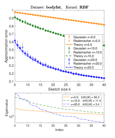
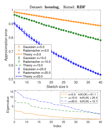
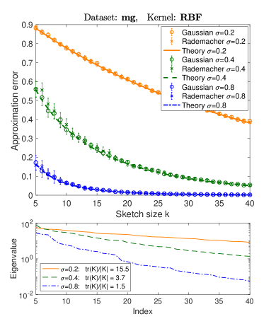
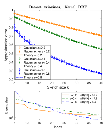
Figure 4: Theoretical predictions versus approximation error for the sketched Nyström with the RBF kernel, using Gaussian and Rademacher sketches (spectral decay shown at the bottom).

Appendix C Additional empirical results

We complement the results of Section 4 with empirical results on four additional libsvm datasets [CL11] (bringing the total number of benchmark datasets to eight), which further establish the accuracy of our surrogate expressions for the low-rank approximation error. Similary as in Figure 2, we use the sketched Nyström method [GM16] with the RBF kernel $k(\mathbf{a}_{i},\mathbf{a}_{j})=\exp(-\|\mathbf{a}_{i}-\mathbf{a}_{j}\|^{2}/(2\sigma^{2}))$, for several values of the parameter $\sigma$. The values of $\sigma$ were chosen so as to demonstrate the effectiveness of our theoretical predictions both when the stable rank is moderately large and when it is very small.

In Figure 4 we show the results for both Gaussian and Rademacher sketches. These results reinforce the conclusions we made in Section 4: our theoretical estimates are very accurate in all cases, for both sketching methods, and even when the stable rank is close to 1 (a regime that is not supported by the current theory).

References

- [Ach03] Dimitris Achlioptas. Database-friendly random projections: Johnson-lindenstrauss with binary coins. Journal of computer and System Sciences, 66(4):671–687, 2003.
- [AM15] Ahmed El Alaoui and Michael W. Mahoney. Fast randomized kernel ridge regression with statistical guarantees. In Proceedings of the 28th International Conference on Neural Information Processing Systems, pages 775–783, 2015.
- [AMT10] Haim Avron, Petar Maymounkov, and Sivan Toledo. Blendenpik: Supercharging lapack’s least-squares solver. SIAM Journal on Scientific Computing, 32(3):1217–1236, 2010.
- [BJ03] Francis R. Bach and Michael I. Jordan. Kernel independent component analysis. J. Mach. Learn. Res., 3:1–48, March 2003.
- [BLLT19] P. L. Bartlett, P. M. Long, G. Lugosi, and A. Tsigler. Benign overfitting in linear regression. Technical Report Preprint: arXiv:1906.11300, 2019.
- [BMD08] Christos Boutsidis, Michael Mahoney, and Petros Drineas. An improved approximation algorithm for the column subset selection problem. Proceedings of the Annual ACM-SIAM Symposium on Discrete Algorithms, 12 2008.
- [BRVDW19] David Burt, Carl Edward Rasmussen, and Mark Van Der Wilk. Rates of convergence for sparse variational Gaussian process regression. In Kamalika Chaudhuri and Ruslan Salakhutdinov, editors, Proceedings of the 36th International Conference on Machine Learning, volume 97 of Proceedings of Machine Learning Research, pages 862–871, Long Beach, California, USA, 09–15 Jun 2019. PMLR.
- [BS10] Zhidong Bai and Jack W Silverstein. Spectral analysis of large dimensional random matrices, volume 20. Springer, 2010.
- [Bur73] Donald L Burkholder. Distribution function inequalities for martingales. the Annals of Probability, pages 19–42, 1973.
- [CEM+15] Michael B. Cohen, Sam Elder, Cameron Musco, Christopher Musco, and Madalina Persu. Dimensionality reduction for k-means clustering and low rank approximation. In Proceedings of the Forty-seventh Annual ACM Symposium on Theory of Computing, STOC ’15, pages 163–172, New York, NY, USA, 2015. ACM.
- [CL11] Chih-Chung Chang and Chih-Jen Lin. LIBSVM: A library for support vector machines. ACM Transactions on Intelligent Systems and Technology, 2:27:1–27:27, 2011.
- [CNW16] Michael B. Cohen, Jelani Nelson, and David P. Woodruff. Optimal approximate matrix product in terms of stable rank. In 43rd International Colloquium on Automata, Languages, and Programming, ICALP 2016, July 11-15, 2016, Rome, Italy, pages 11:1–11:14, 2016.
- [CW17] Kenneth L. Clarkson and David P. Woodruff. Low-rank approximation and regression in input sparsity time. J. ACM, 63(6):54:1–54:45, January 2017.
- [DBPM20] Michał Dereziński, Burak Bartan, Mert Pilanci, and Michael W Mahoney. Debiasing distributed second order optimization with surrogate sketching and scaled regularization. In Advances in Neural Information Processing Systems, volume 33, pages 6684–6695, 2020.
- [DKM20] Michał Dereziński, Rajiv Khanna, and Michael W Mahoney. Improved guarantees and a multiple-descent curve for Column Subset Selection and the Nyström method. In Advances in Neural Information Processing Systems, volume 33, pages 4953–4964, 2020.
- [DL19] Edgar Dobriban and Sifan Liu. Asymptotics for sketching in least squares regression. In Advances in Neural Information Processing Systems, pages 3675–3685, 2019.
- [DLLM20] Michał Dereziński, Feynman Liang, Zhenyu Liao, and Michael W Mahoney. Precise expressions for random projections: Low-rank approximation and randomized newton. In Advances in Neural Information Processing Systems, volume 33, pages 18272–18283, 2020.
- [DLM20] Michał Dereziński, Feynman Liang, and Michael W Mahoney. Exact expressions for double descent and implicit regularization via surrogate random design. In Advances in Neural Information Processing Systems, volume 33, pages 5152–5164, 2020.
- [DM16] Petros Drineas and Michael W. Mahoney. RandNLA: Randomized numerical linear algebra. Communications of the ACM, 59:80–90, 2016.
- [DM18] P. Drineas and M. W. Mahoney. Lectures on randomized numerical linear algebra. In M. W. Mahoney, J. C. Duchi, and A. C. Gilbert, editors, The Mathematics of Data, IAS/Park City Mathematics Series, pages 1–48. AMS/IAS/SIAM, 2018.
- [DM19] Michał Dereziński and Michael W Mahoney. Distributed estimation of the inverse Hessian by determinantal averaging. In H. Wallach, H. Larochelle, A. Beygelzimer, F. d Alché-Buc, E. Fox, and R. Garnett, editors, Advances in Neural Information Processing Systems 32, pages 11401–11411. Curran Associates, Inc., 2019.
- [DM21] Michał Dereziński and Michael W Mahoney. Determinantal point processes in randomized numerical linear algebra. Notices of the American Mathematical Society, 68(1):34–45, 2021.
- [FSS20] Michaël Fanuel, Joachim Schreurs, and Johan AK Suykens. Diversity sampling is an implicit regularization for kernel methods. arXiv:2002.08616, 2020.
- [GKLR19] Robert Gower, Dmitry Koralev, Felix Lieder, and Peter Richtarik. RSN: Randomized subspace Newton. In H. Wallach, H. Larochelle, A. Beygelzimer, F. d Alché-Buc, E. Fox, and R. Garnett, editors, Advances in Neural Information Processing Systems 32, pages 614–623. Curran Associates, Inc., 2019.
- [GM16] Alex Gittens and Michael W. Mahoney. Revisiting the Nyström method for improved large-scale machine learning. J. Mach. Learn. Res., 17(1):3977–4041, January 2016.
- [GR15] Robert M. Gower and Peter Richtárik. Randomized iterative methods for linear systems. SIAM. J. Matrix Anal. & Appl., 36(4), 1660–1690, 2015, 2015.
- [GRB20] Robert Gower, Peter Richtárik, and Francis Bach. Stochastic quasi-gradient methods: variance reduction via Jacobian sketching. Mathematical Programming, 05 2020.
- [HLN+07] Walid Hachem, Philippe Loubaton, Jamal Najim, et al. Deterministic equivalents for certain functionals of large random matrices. The Annals of Applied Probability, 17(3):875–930, 2007.
- [HMRT19] T. Hastie, A. Montanari, S. Rosset, and R. J. Tibshirani. Surprises in high-dimensional ridgeless least squares interpolation. Technical Report Preprint: arXiv:1903.08560, 2019.
- [HMT11] Nathan Halko, Per-Gunnar Martinsson, and Joel A Tropp. Finding structure with randomness: Probabilistic algorithms for constructing approximate matrix decompositions. SIAM review, 53(2):217–288, 2011.
- [LP19] Jonathan Lacotte and Mert Pilanci. Faster least squares optimization. arXiv preprint arXiv:1911.02675, 2019.
- [LPP19] Jonathan Lacotte, Mert Pilanci, and Marco Pavone. High-dimensional optimization in adaptive random subspaces. In Advances in Neural Information Processing Systems, pages 10846–10856, 2019.
- [Mah11] Michael W. Mahoney. Randomized algorithms for matrices and data. Foundations and Trends in Machine Learning, 3(2):123–224, 2011. Also available at: arXiv:1104.5557.
- [Mah12] M. W. Mahoney. Approximate computation and implicit regularization for very large-scale data analysis. In Proceedings of the 31st ACM Symposium on Principles of Database Systems, pages 143–154, 2012.
- [MDK20] Mojmir Mutny, Michał Dereziński, and Andreas Krause. Convergence analysis of block coordinate algorithms with determinantal sampling. In International Conference on Artificial Intelligence and Statistics, pages 3110–3120, 2020.
- [Mey73] Carl D. Meyer. Generalized inversion of modified matrices. SIAM Journal on Applied Mathematics, 24(3):315–323, 1973.
- [MSM14] X. Meng, M. A. Saunders, and M. W. Mahoney. LSRN: A parallel iterative solver for strongly over- or under-determined systems. SIAM Journal on Scientific Computing, 36(2):C95–C118, 2014.
- [NN13] Jelani Nelson and Huy L. Nguyên. Osnap: Faster numerical linear algebra algorithms via sparser subspace embeddings. In Proceedings of the 2013 IEEE 54th Annual Symposium on Foundations of Computer Science, FOCS ’13, pages 117–126, Washington, DC, USA, 2013. IEEE Computer Society.
- [PW16] Mert Pilanci and Martin J Wainwright. Iterative Hessian sketch: Fast and accurate solution approximation for constrained least-squares. The Journal of Machine Learning Research, 17(1):1842–1879, 2016.
- [QR16] Zheng Qu and Peter Richtárik. Coordinate descent with arbitrary sampling II: Expected separable overapproximation. Optimization Methods and Software, 31(5):858–884, 2016.
- [QRTF16] Zheng Qu, Peter Richtárik, Martin Takác, and Olivier Fercoq. SDNA: Stochastic Dual Newton Ascent for Empirical Risk Minimization. Proceedings of The 33rd International Conference on Machine Learning, Feb 2016.
- [RKM19] Farbod Roosta-Khorasani and Michael W Mahoney. Sub-sampled Newton methods. Mathematical Programming, 174(1-2):293–326, 2019.
- [RLXM18] F. Roosta, Y. Liu, P. Xu, and M. W. Mahoney. Newton-MR: Newton’s method without smoothness or convexity. Technical report, 2018. Preprint: arXiv:1810.00303.
- [RM16] G. Raskutti and M. W. Mahoney. A statistical perspective on randomized sketching for ordinary least-squares. Journal of Machine Learning Research, 17(214):1–31, 2016.
- [RV13] Mark Rudelson and Roman Vershynin. Hanson-Wright inequality and sub-gaussian concentration. Electronic Communications in Probability, 18, 2013.
- [RW06] C. E. Rasmussen and C. K. I. Williams. Gaussian Processes for Machine Learning. MIT Press, 2006.
- [Sar06] Tamas Sarlos. Improved approximation algorithms for large matrices via random projections. In Proceedings of the 47th Annual IEEE Symposium on Foundations of Computer Science, FOCS ’06, pages 143–152, Washington, DC, USA, 2006. IEEE Computer Society.
- [Ser10] D. Serre. Matrices: Theory and Applications. Graduate Texts in Mathematics. Springer, 2010.
- [SZW+97] Huaiyu Zhu Santa, Huaiyu Zhu, Christopher K. I. Williams, Richard Rohwer, and Michal Morciniec. Gaussian regression and optimal finite dimensional linear models. In Neural Networks and Machine Learning, pages 167–184. Springer-Verlag, 1997.
- [Ver18] Roman Vershynin. High-dimensional probability: An introduction with applications in data science, volume 47. Cambridge university press, 2018.
- [WGM17] Shusen Wang, Alex Gittens, and Michael W. Mahoney. Sketched ridge regression: Optimization perspective, statistical perspective, and model averaging. In Doina Precup and Yee Whye Teh, editors, Proceedings of the 34th International Conference on Machine Learning, volume 70 of Proceedings of Machine Learning Research, pages 3608–3616, International Convention Centre, Sydney, Australia, 06–11 Aug 2017. PMLR.
- [Woo14] David P. Woodruff. Sketching as a tool for numerical linear algebra. Foundations and Trends® in Theoretical Computer Science, 10(1–2):1–157, 2014.
- [WRXM17] Shusen Wang, Farbod Roosta-Khorasani, Peng Xu, and Michael W. Mahoney. GIANT: globally improved approximate Newton method for distributed optimization. CoRR, abs/1709.03528, 2017.
- [WS01] Christopher K. I. Williams and Matthias Seeger. Using the Nyström method to speed up kernel machines. In T. K. Leen, T. G. Dietterich, and V. Tresp, editors, Advances in Neural Information Processing Systems 13, pages 682–688. MIT Press, 2001.
- [XRKM17] P. Xu, F. Roosta-Khorasani, and M. W. Mahoney. Newton-type methods for non-convex optimization under inexact Hessian information. Technical report, 2017. Preprint: arXiv:1708.07164.
- [YLDW20] Fan Yang, Sifan Liu, Edgar Dobriban, and David P Woodruff. How to reduce dimension with pca and random projections? arXiv preprint arXiv:2005.00511, 2020.
- [YXRKM18] Z. Yao, P. Xu, F. Roosta-Khorasani, and M. W. Mahoney. Inexact non-convex Newton-type methods. Technical report, 2018. Preprint: arXiv:1802.06925.
- [Zaj20] Krzysztof Zajkowski. Bounds on tail probabilities for quadratic forms in dependent sub-gaussian random variables. Statistics & Probability Letters, 167:108898, 2020.