Homogeneity Test for Functional Data based on Data-Depth Plots.

Abstract

One of the classic concerns in statistics is determining if two samples come from the same population, i.e. homogeneity testing. In this paper, we propose a homogeneity test in the context of Functional Data Analysis, adopting an idea from multivariate data analysis: the data depth plot (DD-plot). This DD-plot is a generalization of the univariate Q-Q plot (quantile-quantile plot). We propose some statistics based on these DD-plots, and we use bootstrapping techniques to estimate their distributions. We estimate the finite-sample size and power of our test via simulation, obtaining better results than other homogeneity test proposed in the literature. Finally, we illustrate the procedure in samples of real heterogeneous data and get consistent results.

Keywords: Functional Data Analysis, Data depth, Non-parametric, Bootstrap-t, Hypothesis testing, Robust.

1 Introduction

Functional Data Analysis (FDA) is an area of statistics where functions are the sample elements.  Ramsay (1982) coined the term FDA, but the area is older and dates back to the ’50s (Grenander, 1950; Rao, 1958). With the advance of modern technology, continuously recorded data has become more common and thus interest in the area has spiked. In the FDA context, we consider that certain functions originated the data that we record discretely, and that those functions are the sample members, not the explicit discrete data. Performing some pre-processing steps for smoothing the discrete data is common, but some methods do not need this. For a more complete introduction to FDA refer to (Ramsay and Silverman, 2005; Ferraty and Vieu, 2006), and refer to (Wang et al., 2016; Cuevas, 2014) for reviews of the recent advancements in the area.

FDA usually asks some of the same questions as traditional statistics. Many times we answer these questions by generalizing the existing methods of multivariate statistics to the infinite-dimensional context of functions. Some of the questions we have are: How do we explain this sample using that other sample? How can we summarize this sample? How do we construct a confidence band for this statistic? Do these two samples come from the same population? In this paper, we study the last question by proposing a homogeneity test. If two samples come from the same population they are homogeneous, and they are heterogeneous if they do not. Lets consider the functional samples $\mathcal{F}=\{x_{1},\dots,x_{n}\}$ and $\mathcal{G}=\{y_{1},\dots,y_{m}\}$, defined on the same interval $\mathcal{T}\subset\mathbb{R}$. We assume that the functions lie on $C^{1}(T)$, meaning that their first derivatives are continuous. A homogeneity test looks to contrast that the two samples come from the same distribution or not, i.e. $H_{0}:\mathcal{F}\stackrel{{\scriptstyle d}}{{=}}\mathcal{G}$ or $H_{A}:\mathcal{F}\stackrel{{\scriptstyle d}}{{\neq}}\mathcal{G}$, where $\stackrel{{\scriptstyle d}}{{=}}$ means equality in distribution. In FDA we rarely consider explicit distributions, so we say that two samples are homogeneous when they come from the same ‘parent’ or ‘generator’ process.

Although many homogeneity tests exist for traditional data (see (Szkély, 2002) and (Lung-Yut-Fong et al., 2011) for univariate and multivariate data respectively), there are few for functional data. On the best of our knowledge, the homogeneity test for functional data with the highest power is the one proposed by Flores et al. (2018), but we have evidence that this test has some power problems in certain specific situations, e.g. when samples only differ in covariance structure. See section 4 for a more detailed discussion of this.

The main goal of this paper is to construct some homogeneity tests based on the ideas of multivariate homogeneity using DD-plots proposed by Liu et al. (1999), as well as show that this new tests have greater power than the test proposed by Flores et al. (2018), which is the best homogeneity test for FDA currently in the literature. We evaluate our tests with different simulated data, where we know a priori if the samples are homogeneous or not. First, we will use the same simulation scenarios proposed by Flores et al. (2018), but we will also consider other scenarios.

Since distributions of functional data are rarely considered explicitly, comparing them directly is unfeasible. A good homogeneity test then must compare different aspects of the sample: for example, a good homogeneity test may compare means, variance/covariance structure and curve’s shape simultaneously, while a worse homogeneity test may only compare means between samples. We propose a new homogeneity test that is particularly good at detecting differences between samples in means, variance/covariance structure or in shape of the curves.

The paper is organized as follows. In section 2 we introduce the concept of depth, review different depth measures for functional data and introduce an important homogeneity test found in the literature. Section 3 presents the notion of depth and introduce our depth-based test. Section 4 presents simulation schemes where we compare our tests with others. In section 5 we apply the tests to real data. Section 6 presents the main insights of this paper and future research ideas in homogeneity tests for functional data.

2 Functional Depths

In multivariate statistics, depth measures are generalizations of quantiles, as they provide an inward-out ordering of the data. We use similar ideas in FDA, such as centrality, shape, or closeness to other functions to propose depth measures. Different notions of depth for functional data explore different such features. Akin to multivariate depths, we can interpret the deepest function on a sample as the median of that sample. In this section we will consider samples $\mathcal{F}=\{x_{1},\dots,x_{n}\}$ in an interval $\mathcal{T}$.

Fraiman and Muniz (2001) introduced the first notion of functional depth. The idea behind this notion is to measure how much ‘time’ each function is deep inside the sample, i.e., how surrounded is the function by other functions. Their idea is to measure univariate depths for each $t\in\mathcal{T}$, and the deepest function is the function which on average maximizes this value. More formally, fix a $t_{o}\in\mathcal{T}$ and consider the univariate depth $D_{n}(x_{i}(t_{0}))$, and define the Fraiman-Muniz depth as

$$FM(x_{i}(t))=\int_{\mathcal{T}}D_{n}(x_{i}(t))dt,$$

that is, the average of the depths for all $t_{0}\in\mathcal{T}$. Note that $D_{n}$ can be any notion of univariate depth. In particular, we choose

$$D_{n}(x_{i}(t_{0}))=1-\left|\frac{1}{2}-F_{n,t}(x_{i}(t_{0}))\right|,$$

where $\hat{F}_{n,t_{0}}$ is the empirical CDF of $x_{1}(t_{0}),\dots,x_{n}(t_{0})$.

The Random Projection depth (Cuevas et al., 2007) considers univariate random projections of the functions. The RP depth is then the average of the corresponding univariate depths of the projections. More formally, consider the projection of $x_{i}$ along direction $v$ as

$$r_{i,v}(x_{i}(t))=\int_{\mathcal{T}}v(t)x_{i}(t)dt,$$

and consider $p$ realizations of $v$. The $p$ univariate projections of $x_{i}$ are $r_{i,1},\dots,r_{i,p}$. Consider this notion of univariate depth for the projections

$$d_{i,j}=\min\{\hat{F}_{n}(r_{i,j}),1-\hat{F}_{n}(r_{i,j})\},$$

where $\hat{F}_{n}$ is the empirical distribution function of all the functions projected against the same realization of $v$, i.e., if we are in the $j$th realization of $v$, $\hat{F}_{n}$ is the empirical distribution of $r_{1,j},\dots,r_{p,j}$. Now, the RP depth is the mean of those univariate depths for each function, i.e.

$$RPD(x_{i}(t))=\frac{1}{p}\sum_{j=1}^{p}d_{i,j}.$$

The deepest function will be the one that, on average, is deeper in its random univariate projections. In this work, we use $50$ projections of $v$ to compute the RP depth.

Nagy et al. (2017) warn that traditional functional depths are very simplistic and do not take into account the shapes of the functions or the covariance structure of the sample. They argue that usual functional depths are analogous to taking only coordinate-wise medians in multivariate samples, and interpreting that as the median of the sample, which is ill-advised (Rousseeuw and Ruts, 1999) since the idea of the depths is to capture global features of the sample’s probability distribution rather than local features (Paindaveine and bever, 2013). Then, they propose a $J$-th ordered integrated depth that can capture global features of the sample as

$$FD_{J}(x_{i}(t);P)=\int_{\mathcal{T}}\dots\int_{\mathcal{T}}D\left((x_{i}(t_{1}),\dots,x_{i}(t_{J})^{T});P_{\left(X(t_{1}),\dots,X(t_{J})\right)^{T}}\right).$$

where $P$ is a probability measure in the functional space, $D$ is a depth measure in a finite space of dimension $J$, and $P_{\left(X(t_{1}),\dots,X(t_{J})\right)^{T}}$ is the corresponding probability measure in that finite space. To compute $FD_{J}$, fix a $J$ and plug-in the corresponding empirical measure $P_{n}$ for $P_{\left(X(t_{1}),\dots,X(t_{J})\right)^{T}}$ and select a $J$-dimensional depth $D$. In this work we set $J=2$ and the half-space depth proposed by Tukey (1975).  Nagy et al. (2017) establish connections from the $J$-th ordered depth to the $J-1$-th derivative of the data: that means that the $2$nd ordered depths brings us information about the shape of the curve (first derivative) and the $3$rd ordered depths brings us information about the convexity of the curve (second derivative).

Other depth functions use different features of the curves. For example, the h-modal depth generalizes the notion of modes to functional data (Cuevas et al., 2006). López-Pintado and Romo (2009) define the band depth, which measures how much each curve is contained in the ‘band’ generated by any other functions in the sample, where a band is a part of the plane delimited by any number of function. The deepest function is then the one which is contained in more bands.

Flores et al. (2018) define a homogeneity test based on these notions of depths. Their goal is to propose a measure of the distance between samples of functional data. Let $\mathcal{F}$ and $\mathcal{G}$ be the two samples we want to test for homogeneity. Denote $d_{\mathcal{F}}(g)$ the depth of $g$ in a sample $\mathcal{F}\cup g$, and define $\mathcal{D}_{\mathcal{F}}(\mathcal{G})$ as the function which maximizes $d_{\mathcal{F}}(g)$ among $g\in G$. They propose the following statistics:

$$P_{1}(\mathcal{F},\mathcal{G}) =d_{\mathcal{F}}\mathcal{D}_{\mathcal{G}}\mathcal{G},$$

$$P_{2}(\mathcal{F},\mathcal{G}) =P_{1}(\mathcal{F},\mathcal{F})-P_{1}(\mathcal{F},\mathcal{G}),$$

$$P_{3}(\mathcal{F},\mathcal{G}) =d_{\mathcal{F}}\mathcal{D}_{\mathcal{F}}\mathcal{G},$$

$$P_{4}(\mathcal{F},\mathcal{G}) =|P_{3}(\mathcal{F},\mathcal{G})-P_{1}(\mathcal{F},\mathcal{F})||P_{3}(\mathcal{F},\mathcal{G})-P_{1}(\mathcal{G},\mathcal{G})|.$$

The idea behind $P_{1}$ is that the function $\mathcal{D}_{\mathcal{G}}\mathcal{G}$ is the most representative element of $\mathcal{G}$, so then if its depth is big in $\mathcal{F}$, it is most likely that $\mathcal{F}$ and $\mathcal{G}$ are in the same family, i.e., that they are homogeneous. The idea behind $P_{3}$ is that if the function of $\mathcal{G}$ most likely to come from the experiment $\mathcal{F}$ is very deep in $\mathcal{F}$, then the two experiments will likely be very mixed and thus come from the same population. $P_{2}$ and $P_{4}$ are normalizations of $P_{1}$ and $P_{3}$. Then they use these statistics and bootstrapping techniques to test the $H_{0}$ of homogeneity.

3 DD-plots and their relation with homogeneity

Multivariate data analysis influences FDA. For example, depth measures, first proposed for multivariate data, have been adapted to a functional context, where it has been succesfully applied. For example,  Sun and Genton (2011) proposed a generalization of boxplots for FDA, called the Functional Boxplot. DD-plots have been also adapted for FDA but in the context of classification (Cuesta-Albertos et al., 2017).

Liu et al. (1999) introduced the notion of DD-plots, which are a way of comparing multivariate distributions of two samples using depth measures. Let $\mathcal{F}=\{x_{1},\dots,x_{n}\}$ and $\mathcal{G}=\{y_{1},\dots,y_{m}\}$ be the two samples we want to test for homogeneity, and let $\mathcal{H}=\mathcal{F}\cup\mathcal{G}$. Define the DD-plot of the combined sample as $DD(\mathcal{F},\mathcal{G},\mathcal{H})=\{(D_{\mathcal{F}}(x),D_{\mathcal{G}}(x)),x\in\mathcal{H}\}$ where $D$ is an arbitrary depth function in any of the sample spaces $\mathcal{F}$ or $\mathcal{G}$. Then $DD(\mathcal{F},\mathcal{G},\mathcal{H})$ is a set of pairs of size $|\mathcal{H}|=n+m$.

Following this idea, since depths try to characterize the distributions of samples, they propose that DD-plots between homogeneous samples must be similar to the identity, that is, the scatter plot generated by the DD-plot should concentrate towards the $(0,0)-(1,1)$ line. Figure 1 shows DD-plots for homogeneous and heterogeneous samples.

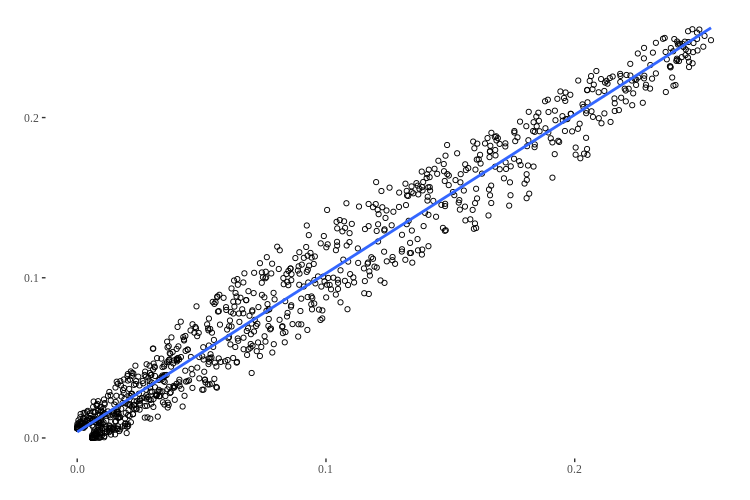
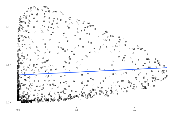
Figure 1: DD-plots for multivariate data. The DD-plot on the left is for homogeneous samples, where both samples were generated as $N(\bm{0},I)$. The DD-plot in the right is for heterogeneous samples, where the first sample was generated with $N(\bm{0},I)$ and the second sample was generated with $N(\bm{\mu},\Sigma)$, where $\bm{\mu}=[0.5,1.3]$ and $\Sigma=\bigl{(}\begin{smallmatrix}1.5&0.3\\ 0.3&1.5\end{smallmatrix}\bigr{)}$. The Depth function used is the Simplicial Depth (Liu, 1990). The homogeneous DD-plot stays concentrated towards the $(0,0)-(1,1)$ line and the heterogeneous is dispersed.

Our main idea is to use the proposed relationship presented in  Liu et al. (1999) between homogeneity and DD-plots, and propose some statistics that can capture how concentrated the DD-plot is towards the $(0,0)-(1,1)$ diagonal. It is worth noting that DD-plots are depth agnostic and you construct them using any notion of depth. An introduction to the functional depths that we use in this work is in Section 2.

If the same process generated the two samples then the DD-plot should concentrate towards the $(0,0)-(1,1)$ diagonal line. To test this, we consider.

$$D_{\mathcal{F},i}=\beta_{0}+\beta_{1}D_{\mathcal{G},i}+u_{i}\quad\forall i=1,2,\dots,n+m,$$ (1)

with $u_{i}$ being the usual error. We want to test that $\beta_{0}=0$ and $\beta_{1}=1$, which gives us an idea of how the points concentrate towards the $(0,0)-(1,1)$ diagonal line.

We will be testing using bootstrap-t, which has second-order convergence properties (DiCiccio and Efron, 1996). Testing with the traditional t-test is not reasonable as the normality assumption of $u_{i}$ does not hold: the values of $D_{\mathcal{F},i}$ and $D_{\mathcal{G},i}$ lie inside $[0,1]$ by definition, so by regressing one against the other, we will get that $[-1,1]$ bounds $u_{i}$, and thus it is not normally distributed, as the normal distribution is not bounded.

Let us say we want to propose a test for a parameter $\theta$, and we want to check if $\theta=\theta_{0}$ Suppose that, with the sample $\bm{X}$, we can estimate $\hat{\theta}$ and $\hat{\sigma}$, the standard deviation of $\hat{\theta}$. Following Wald’s test, define the test statistic

$$T=\frac{\hat{\theta}-\theta_{0}}{\hat{\sigma}}.$$ (2)

We want to estimate a distribution for $T$. Draw bootstrap samples under the $H_{0}$ from $\bm{X}$. Call them $\bm{X}^{*}$, which yields a $\hat{\theta}^{*}$ and a $\hat{\sigma}^{*}$. And with those, we can estimate the bootstrap replications of $T$ as

$$T^{*}=\frac{\hat{\theta}^{*}-\theta_{0}}{\hat{\sigma}^{*}}.$$ (3)

Now, using this bootstrap-t we will check if $\beta_{0}=0$ and $\beta_{1}=1$ for the DD-plot. First, compute $DD(\mathcal{F},\mathcal{G},\mathcal{H})$, and get the least square estimates of the parameters in equation 1: $\hat{\beta}_{1}$ and $\hat{\beta}_{0}$. Also, compute the standard error of these parameters, given by (See (Seltman, 2018, p. 224))

$$\hat{\sigma}_{\beta_{0}} =\sqrt{\frac{\sum_{i=1}^{n+m}\hat{u}_{i}^{2}\sum_{i=1}^{n+m}D_{\mathcal{G},i}}{(n+m-2)\sum_{i=1}^{n+m}(D_{\mathcal{G},i}-\bar{D}_{\mathcal{G}})}},$$

$$\hat{\sigma}_{\beta_{1}} =\sqrt{\frac{\sum_{i=1}^{n+m}\hat{u}_{i}^{2}}{(n+m-2)\sum_{i=1}^{n+m}(D_{\mathcal{G},i}-\bar{D}_{\mathcal{G}})}},$$

where $\hat{u}_{i}$ are the estimated residuals and $\bar{D}_{\mathcal{G}}$ is the mean of the $D_{\mathcal{G},i}$. You can now use equation 2 to compute

$$T_{0} =\frac{\hat{\beta}_{0}}{\hat{\sigma}_{\beta_{0}}},$$

$$T_{1} =\frac{\hat{\beta}_{1}-1}{\hat{\sigma}_{\beta_{1}}},$$

which are the test statistics. Then, since in the null hypothesis $\mathcal{F}\stackrel{{\scriptstyle d}}{{=}}\mathcal{G}$, resample $\mathcal{H}$ with replacement to get $\mathcal{H}^{*}$. Compute the $DD(\mathcal{F},\mathcal{G},\mathcal{H}^{*})$ points, and use them to compute $T^{*(i)}_{0}$, $T^{*(i)}_{1}$, $i\in\{1,\dots,B\}$ bootstrap replicates of each test statistic. Now, estimate the p-values of the test as

$$p_{0} =2\min\bigg{\{}\frac{1}{B}\sum_{i=1}^{B}I(T^{*(i)}_{0}>T_{0}),\frac{1}{B}\sum_{i=1}^{B}I(T^{*(i)}_{0}<T_{0})\bigg{\}},$$

$$p_{1} =2\min\bigg{\{}\frac{1}{B}\sum_{i=1}^{B}I(T^{*(i)}_{1}>T_{1}),\frac{1}{B}\sum_{i=1}^{B}I(T^{*(i)}_{1}<T_{1})\bigg{\}},$$

where $I(\cdot)$ is the indicator function.

Select an appropriate confidence level $\alpha$. In this work, we consider $\alpha=0.05$ Since we have two p-values, we need to use a sequentially rejective multiple test to ensure a size $\alpha$ in our test. Using the Holm-Bonferroni method proposed by Holm (1979), we order the $p$ ascendingly, getting $p_{[1]},p_{[2]}$. Finally, reject the test if $p_{[1]}<\alpha/2$ or $p_{[2]}<\alpha$, and do not reject otherwise. The adjusted p-value of the test will then be $p=\min\{2p_{[1]},p_{[2]}\}$.

4 Simulation studies

In this section, we will compute the empirical power and size of the tests proposed in this work and the test proposed by Flores et al. (2018). For conciseness, from now on we will refer to that test as ‘Flores test’, using $P_{4}$ with FM depth, since that was their best performer, power-wise, in their paper. Let us call as DD-FM test, DD-RP test, and DD-$FD_{J}$ the DD-plot based tests with Fraiman-Muniz, Random Projection, and $FD_{J}$ depths respectively, as described in section 3.

We generate samples from two models and count the proportion of rejections. If the same model generated the two samples, this measures finite-sample size, and if two different models generated the two samples, this measures finite-sample power. The finite-sample size should be near the chosen significance level, and the finite sample-power should be as big as possible.

The models we propose are of the form of equation 4, where $\mu(t)$ is the mean function of the process $x(t)$, $\delta>0$ is a scalar difference between means of processes; and $e_{i}(t)$ is a stochastic Gaussian process with zero mean and covariance function $\gamma(s,t)=ce^{-c|t-s|}$, where $s,t\in[0,1]$ and $k,c>0$. Bigger values of $k$ generate smoother curves, and bigger values of $c$ generate more irregular functions.

$$x_{i}(t)=\mu(t)+\delta+e_{i}(t).$$ (4)

Our simulation procedure is based on the procedure proposed by Flores et al. (2018). They consider 6 different models, from which they generate samples of 50 curves, and compare samples generated from the first model to samples of the same model and to the other 5. Different parameters in equation 4 generate these different models:

• Model 0: $\mu(t)=30t^{3/2}(1-t)$, $\delta=0$ and $\gamma(s,t)=0.3exp(-3.33|t-s|)$.

• Model 1: $\mu(t)=30t^{3/2}(1-t)$, $\delta=1$ and $\gamma(s,t)=0.3exp(-3.33|t-s|)$.

• Model 2: $\mu(t)=30t^{3/2}(1-t)$, $\delta=0.5$ and $\gamma(s,t)=0.3exp(-3.33|t-s|)$.

• Model 3: $\mu(t)=30t{(1-t)}^{2}$, $\delta=0$ and $\gamma(s,t)=0.3exp(-3.33|t-s|)$.

• Model 4: $\mu(t)=30t{(1-t)}^{2}$, $\delta=0$ and $\gamma(s,t)=0.5exp(-5|t-s|)$.

• Model 5: $\mu(t)=30t^{3/2}(1-t)$, $\delta=0$ and $\gamma(s,t)=0.5exp(-5|t-s|)$.

In Figure 2 there are samples of the models described. The first $5$ graphs show two samples generated by different models. The last graph shows two different samples generated from model $0$. A good homogeneity test should reject homogeneity in the first five examples, and not reject homogeneity in the last example.

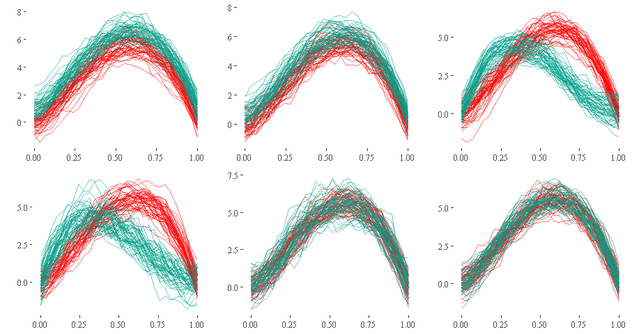
Figure 2: The first five plots are realizations of the reference population in red vs realization of another population in green. The sixth plot is two realizations of model zero. Some changes between samples can be seen easily (first or third plot), but others are quite hard to spot (the last two plots are almost indistinguishable, but the fifth is of heterogeneous samples and the sixth of homogeneous samples).

DD-plots for the samples in figure 2 can be found in figures 3, 4, and 5. In the first four cases, the samples are heterogeneous as the points are not concentrated toward the the $(0,0)-(1,1)$ diagonal line. It is trickier to say if the samples are heterogeneous in the next two cases: the DD plots seem that of homogeneous samples (and that is not true for the fifth figure), so it is better to perform our proposed homogeneity test to have more certainty.

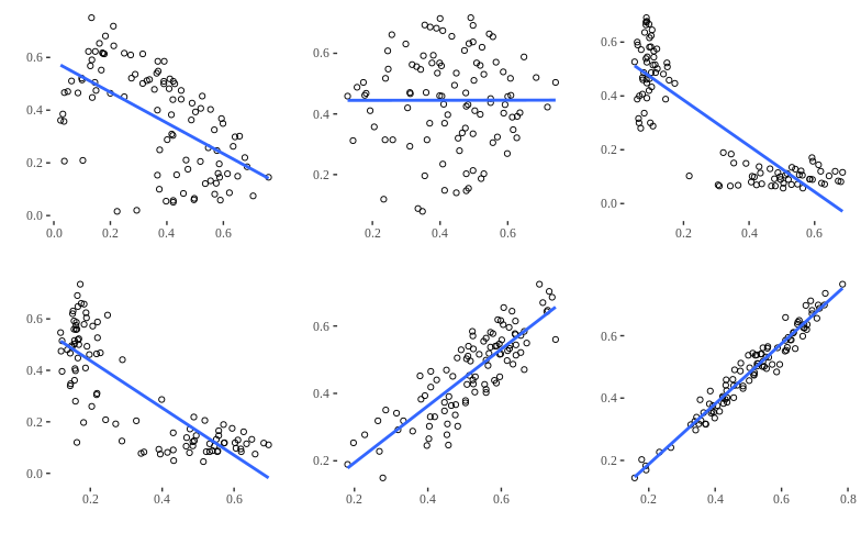
Figure 3: DD-plots using the FM depth for samples of the 6 models mentioned, all compared with Model 0.

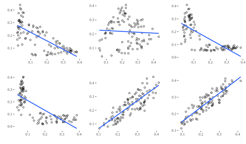
Figure 4: DD-plots using the RP depth for samples of the 6 models mentioned, all compared with Model 0.

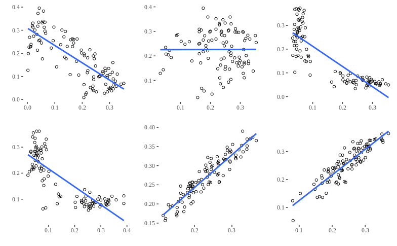
Figure 5: DD-plots using the $FD_{J}$ depth for samples of the 6 models mentioned, all compared with Model 0.

Table 1 summarizes finite sample powers and sizes. All tests achieved good size since all have values near the significance level chose, $\alpha=0.05$. The only test that had an average size bigger than $\alpha$ was the Flores Test, with $0.053$. This means that DD-plot based tests were better size-wise, with both the DD-FM test and the DD-$FD_{J}$ test having maximum sizes less than $\alpha$, so it is likely that we will not reject $H_{0}$ when it is true. Power-wise, the DD-plot based tests were the best performers, with all having a bigger average and minimum power than the Flores’ test. The best performer was the DD-$FD_{J}$ test: it has the biggest average and minimum power, meaning that on average it performs very well and that its worst performance was still quite good. Part of its success is that it works very well in instances where the change between samples was in the mean (all tests were able to reject $H_{0}$ in these cases), but also could detect when samples differ only in covariance structure, which the other test could not achieve. This could mean that the claims of Nagy et al. (2017) are true, and this depth can capture global features of the sample’s distribution better than the other depths.

Test	Average size	Maximum size	Average power	Minimum power
Flores Test	0.053	0.07	0.785	0.07 (3v4)
DD-FM	0.023	0.04	0.939	0.57 (3v4)
DD-RP	0.023	0.06	0.93	0.53 (0v5)
DD-$FD_{J}$	0.023	0.05	0.968	0.82 (3v4)

Table 1: Summary of the results for each test. The minimum power column also contains which models were being compared when that power was obtained. The DD-$FD_{J}$ has the biggest power and a very good size

Some differences between models depend only on certain parameters, e.g. model $0,1$ and $2$ only differ in their values of $\delta$. We can then begin changing this parameter to know what is the breaking point of our tests, i.e., how small can be $\delta$ for the tests to still detect heterogeneity. DD-plots for different values of $\delta$ are in Figure 6, where you can note that as $\delta$ gets bigger, the DD-plots present greater deviation from the $(0,0)-(1,1)$ line, which is what you would expect. Figure 7 summarizes the simulation experiments of this scenario. You can see that the Flores Test can detect earlier the change in $\delta$, meaning that this test is the best homogeneity test when populations differ in the mean by a certain scalar. Also, as expected, the average p-values across $100$ tests tend to be lower as $\delta$ increases.

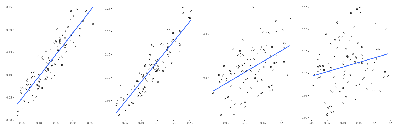
Figure 6: DD-plots with the $FD_{J}$ depth when $\delta$ is increasing.

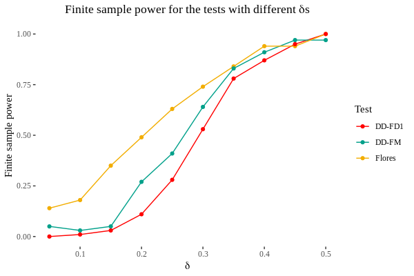
Figure 7: Power of each test when $\delta$ is increasing, generating more disperse DD-plots. The Flores Test is able to detect subtle changes in $\delta$ more easily.

On the other hand, models $0,5$ and models $4,5$ differ only in the variance/covariance structure. We can evaluate a similar scenario by changing another parameter: Consider two models that only differ in k, given by equation 4 , i.e., two models that only differ in covariance structure. The first model will have a fixed $k=0.3$, and the second model will have a $k=0.3m$, with $m$ changing. The models will be homogeneous when $m=1$, and heterogeneous otherwise. Let us examine when the different tests have good power with different values of $m$. In figure 8 you can see the change in DD-plots corresponding to the changes in $m$: with small values or large values of $m$, the plots present behaviors of non-homogeneous samples, which is what you would expect. Figure  9 summarizes the simulation experiments of this scenario. You can see that the Flores Test is not able to detect the changes in m, while the DD-based tests can get very good powers with subtle changes in m. The best test in this scenario was the DD-$FD_{J}$ test, which reaches perfect sample power quicker than the other tests.

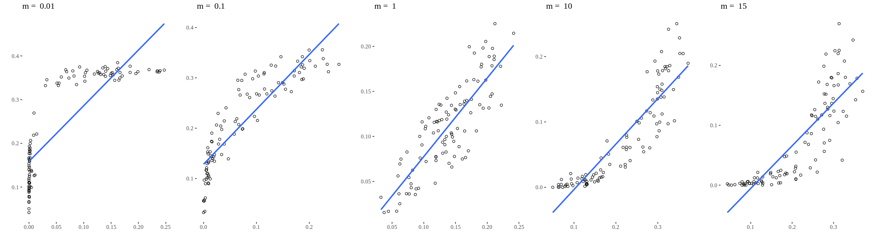
Figure 8: DD-plots with the $FD_{J}$ depth when $m$ is changing. As m decreases or increases much we see some patterns of deviation from the $(0,0)-(1,1)$ diagonal line.

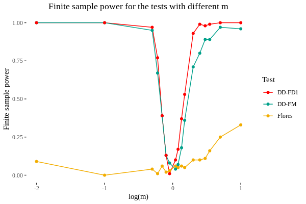
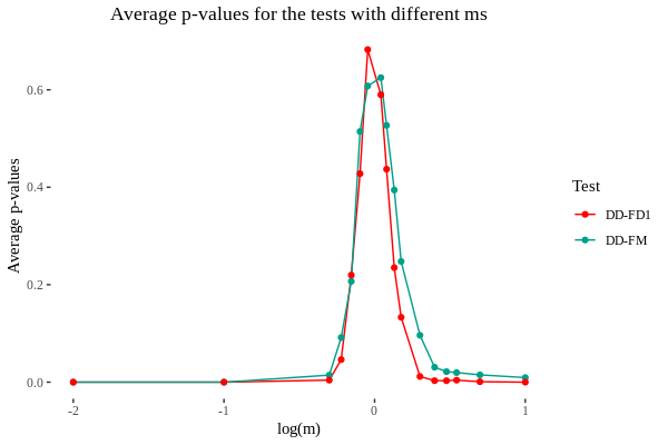
Figure 9: Power of each test when m changes. The Flores Test is not able to detect this changes, and the DD-$FD_{J}$ is able to detect them quite easily.

5 Detecting heterogeneity in samples of real data

In this section, we will consider several data-sets of functional data. They consist of two heterogeneous groups, so our tests should reject the null hypothesis that they are homogeneous.

The first set of curves we are considering is the Berkeley Growth Data, which contains the heights of 39 boys and 54 girls from ages 1 to 18. It is well known that growth dynamics differ from boys to girls, so our test should reject the null hypothesis of homogeneity. You can see the curves in figure 10. In figure 11, you can see the DD-plots obtained from these two samples using different depths, which show behavior typical of heterogeneous samples: they are not concentrated towards the $(0,0)-(1,1)$ diagonal line.

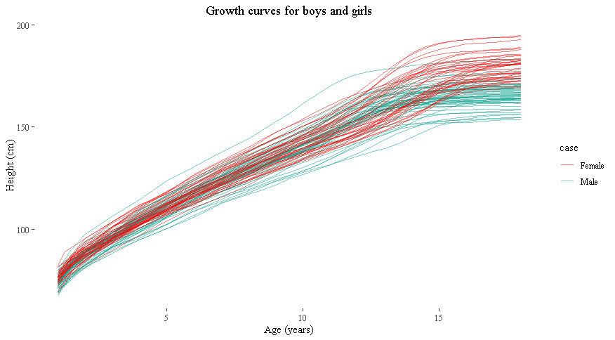
Figure 10: Berkeley Growth Data. Green for males and red for females.

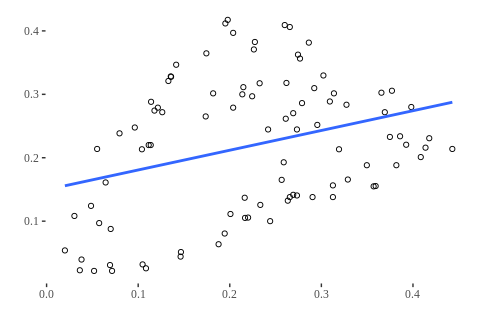
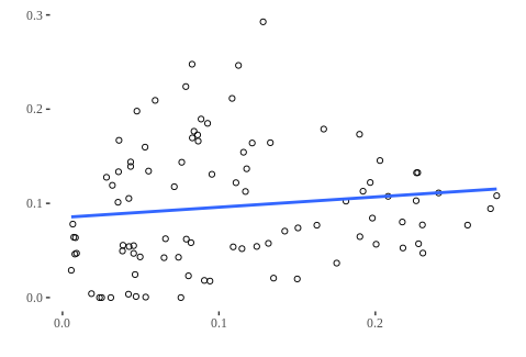
Figure 11: DD plots for the height curves of boys and girls. From left to right they use the FM depth, the RP depth and the $FD_{J}$ depth.

The Tecator data-set consists of spectrometric curves for chopped pieces of meat, which correspond to the absorbance measured at $100$ different wavelengths. We can divide these meats into groups, according to Ferraty and Vieu (2006): the pieces with small and big fat percentages (where small is less than $20\%$ fat). The curves are in figure 12. The DD-plots using different depths of these samples are in figure 13. The points do not concentrate on the $(0,0)-(1,1)$ diagonal line.

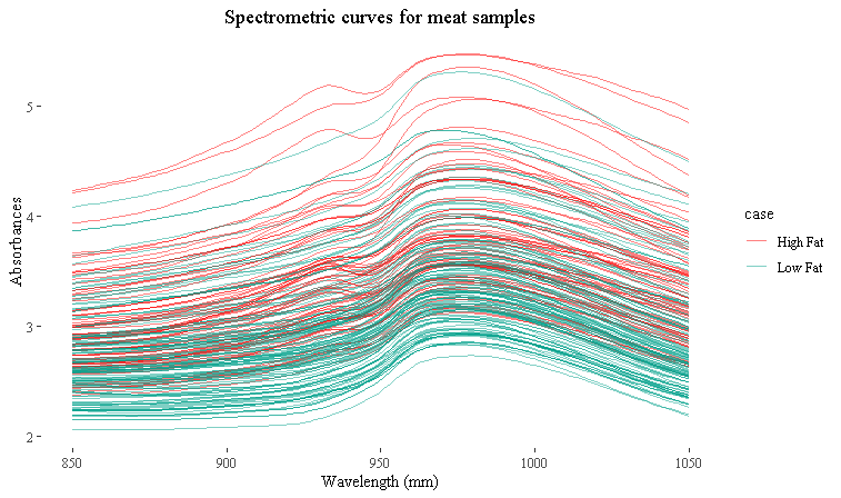
Figure 12: Tecator Spectrometry Data. Green for low-fat meat and red for high-fat meat.

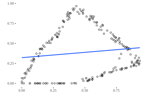
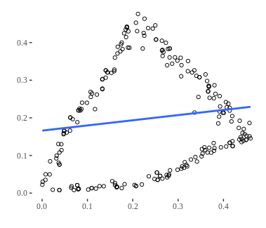
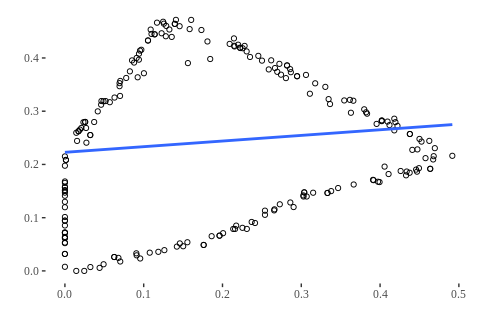
Figure 13: DD plots for spectrometric curves of low and high fat containing meats. From left to right they use the FM depth, the RP depth, and the $FD_{J}$ depth.

Febrero et al. (2008) propose a dataset measuring nitrogen oxide emission levels in a control station in Poblenou, a neighborhood in Barcelona. The station measures $NO_{x}$ levels in $\mu g/m^{3}$ every hour, every day. They split curves into two groups: working days and non-working days. The curves are in Figure 14, and their respective DD-plots using various depths are in Figure 15. Once more, you can see that the points are not concentrated toward the $(0,0)-(1,1)$ line.

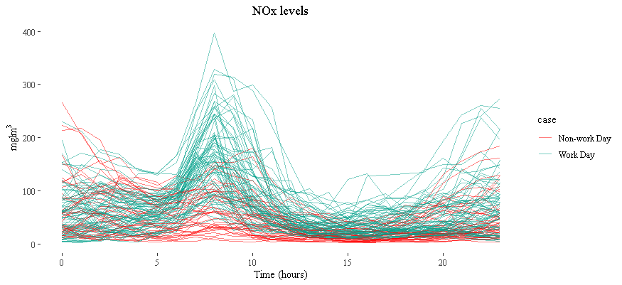
Figure 14: Curves for $NO_{x}$ levels in a Barcelona Neighborhood for work and non-work days.

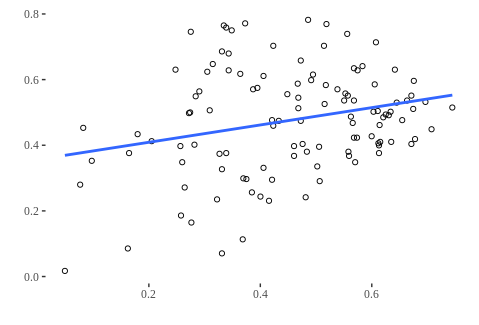
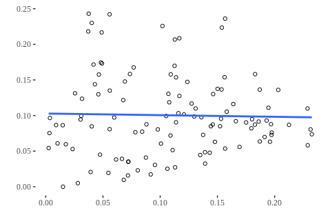
Figure 15: DD-plots for the $NO_{x}$ curves in Poblenou for work and non-work days. From left to right they use the FM depth, the RP depth, and the FDJ depth.

Finally, let us consider the Mitochondrial calcium overload (MCO) data-set. During ischemic myocardia, high levels of MCO relate to better protection against ischemia. Then, it is interesting to see if some drugs can raise MCO levels in rats. This database consists of two groups: one which receives no drug; and another group that receives a drug that can raise MCO levels. Every $10s$ they measure MCO levels. See (Ruiz-Meana et al., 2003) for the complete description of the experiment. In figure 16 we can see both populations. The DD-plots of these samples are in figure 17. The points do not concentrate on the $(0,0)-(1,1)$ line.

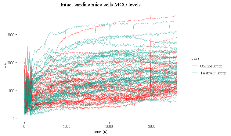
Figure 16: Curves for MCO levels in mouses’ cardiac cells. One sample is the control sample and the other is treated with a certain drug.

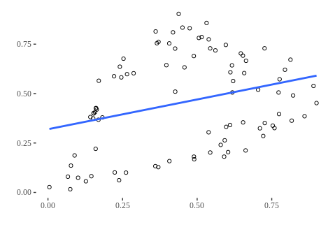
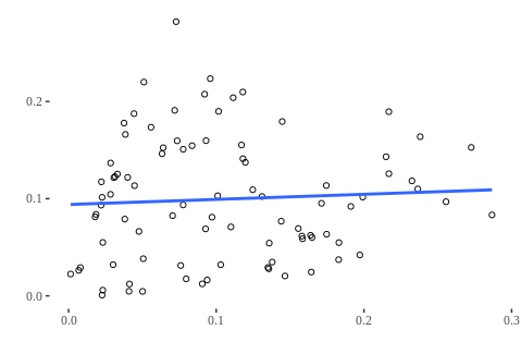
Figure 17: DD plots for the MCO curves in mouse’s cardiac cells, one group treated with a drug and the other used for control. From left to right they use the FM depth, the RP depth, and the FDJ depth.

Yet, performing a visual check for homogeneity using DD-plots is not satisfactory enough, as we do not get important metrics like the p-value. Performing then the tests proposed in this paper, we get the results in table 2. The DD-$FD_{J}$ test was the only test that was able to reject $H_{0}$ in all the cases, getting very small p-values. The Flores Test was only able to reject $H_{0}$ half the times. Both the DD-FM and the DD-RP tests were able to reject $H_{0}$ in all the cases except one.

Data-set	Flores’ Test	DD-FM Test	p	DD-RP Test	p	DD-$FD_{J}$ Test	p
Heights	✗	✗	0.324	✗	0.268	✓	0.00
Tecator	✓	✓	0.034	✓	0.096	✓	0.00
MCO	✓	✗	0.072	✓	0.176	✓	0.00
NOx	✗	✓	0.32	✓	0.28	✓	0.00

Table 2: Result of the tests in the data-sets considered. This ✓ means that the test was able to reject $H_{0}$ and the ✗ means that it did not reject $H_{0}$. The DD-$FD_{J}$ was able to detect accurately reject $H_{0}$ with near $0$ $p$-values always.

6 Discussions and conclusions

In this article, we proposed a homogeneity test for functional data using DD-plots. We adapted the idea linking multivariate DD-plots and homogeneity, proposed by Liu et al. (1999) to a functional setting. We then formalized these notions into a test that considers a linear model for the DD-plot, and using bootstrap-t, tests two linear hypotheses that relate to homogeneity between samples. We handle the multiple hypotheses using the Holm-Bonferroni method.

This proposal compares in its entirety the depth measures between two samples, making it robust to many scenarios, and this is the advantage of our method. Other tests, like (Flores et al., 2018), compares only the most representative datum between samples. Also, this test used bootstrap-t procedures, which are second-order accurate (DiCiccio and Efron, 1996), better than the classic bootstrap confidence intervals which are only first-order accurate.

We compared our tests’ and other tests’ finite-sample performances through simulation. Our test achieved a desirable finite-sample size, and finite-sample power was greater than the finite-sample power of other tests found in the literature in many different scenarios. The test achieved particularly good results when the difference between samples is only in covariance, and other tests have poor finite-sample power for this scenario.

Our tests results in real data-sets were also satisfactory: in every case, the results obtained were concordant with reality, while other tests were not able to do that.

We can extend the methods in this article in several ways: We can change the bootstrap-t for another re-sampling method. Also, we could propose a non-parametric version of the F statistic, used for multiple lineal hypothesis testing. We could implement different depth measures that were not considered here, like (Narisetty and Nair, 2016), to asses their finite-sample power. We could consider other simulation scenarios: can our test detect heterogeneity when the samples have the same means and covariance operators but have different kurtosis? Walter (2011) proposes some kurtosis measures for FDA, and we can create new simulation scenarios based on them.

7 Acknowledgments

The authors gratefully acknowledge Universidad EAFIT, as this article is a part of the project Statistical homogeneity test for infinite-dimensional data, funded by the university.

SUPPLEMENTARY MATERIAL

methods.zip:

File containing the implementation of Flores et al. (2018) method and of the method described in this paper, as well as a script that simulates data as described in this paper.

References

- Cuesta-Albertos et al. (2017) Cuesta-Albertos, J. A., M. Febrero-Bande, and M. Oviedo de la Fuente (2017, Mar). The ddg-classifier in the functional setting. TEST 26(1), 119–142.
- Cuevas (2014) Cuevas, A. (2014). A partial overview of the theory of statistics with functional data. Journal of Statistical Planning and Inference 147, 1 – 23.
- Cuevas et al. (2006) Cuevas, A., M. Febrero, and R. Fraiman (2006, November). On the use of the bootstrap for estimating functions with functional data. Comput. Stat. Data Anal. 51(2), 1063–1074.
- Cuevas et al. (2007) Cuevas, A., M. Febrero, and R. Fraiman (2007, Sep). Robust estimation and classification for functional data via projection-based depth notions. Computational Statistics 22(3), 481–496.
- DiCiccio and Efron (1996) DiCiccio, T. J. and B. Efron (1996, 09). Bootstrap confidence intervals. Statist. Sci. 11(3), 189–228.
- Febrero et al. (2008) Febrero, M., P. Galeano, and W. González-Manteiga (2008). Outlier detection in functional data by depth measures, with application to identify abnormal nox levels. Environmetrics 19(4), 331–345.
- Ferraty and Vieu (2006) Ferraty, F. and P. Vieu (2006). Nonparametric Functional Data Analysis: Theory and Practice. Springer Series in Statistics. Springer.
- Flores et al. (2018) Flores, R., R. Lillo, and J. Romo (2018). Homogeneity test for functional data. Journal of Applied Statistics 45(5), 868–883.
- Fraiman and Muniz (2001) Fraiman, R. and G. Muniz (2001). Trimmed means for functional data. Test 10(2), 419–440.
- Grenander (1950) Grenander, U. (1950, 10). Stochastic processes and statistical inference. Ark. Mat. 1(3), 195–277.
- Holm (1979) Holm, S. (1979). A simple sequentially rejective multiple test procedure. Scandinavian Journal of Statistics 6(2), 65–70.
- Liu (1990) Liu, R. Y. (1990, 03). On a notion of data depth based on random simplices. Ann. Statist. 18(1), 405–414.
- Liu et al. (1999) Liu, R. Y., J. M. Parelius, and K. Singh (1999). Multivariate analysis by data depth: Descriptive statistics, graphics and inference. The Annals of Statistics 27(3), 783–840.
- Lung-Yut-Fong et al. (2011) Lung-Yut-Fong, A., C. Lévy-Leduc, and O. Cappé (2011, Jul). Homogeneity and change-point detection tests for multivariate data using rank statistics. arXiv e-prints 0(0), arXiv:1107.1971.
- López-Pintado and Romo (2009) López-Pintado, S. and J. Romo (2009). On the concept of depth for functional data. Journal of the American Statistical Association 104(486), 718–734.
- Nagy et al. (2017) Nagy, S., I. Gijbels, and D. Hlubinka (2017). Depth-based recognition of shape outlying functions. Journal of Computational and Graphical Statistics 26(4), 883–893.
- Narisetty and Nair (2016) Narisetty, N. N. and V. N. Nair (2016). Extremal depth for functional data and applications. Journal of the American Statistical Association 111(516), 1705–1714.
- Paindaveine and bever (2013) Paindaveine, D. and G. V. bever (2013). From depth to local depth: A focus on centrality. Journal of the American Statistical Association 108(503), 1105–1119.
- Ramsay and Silverman (2005) Ramsay, J. and B. W. Silverman (2005). Functional Data Analysis. Springer Series in Statistics. Springer.
- Ramsay (1982) Ramsay, J. O. (1982, Dec). When the data are functions. Psychometrika 47(4), 379–396.
- Rao (1958) Rao, C. R. (1958). Some statistical methods for comparison of growth curves. Biometrics 14(1), 1–17.
- Rousseeuw and Ruts (1999) Rousseeuw, P. J. and I. Ruts (1999, Oct). The depth function of a population distribution. Metrika 49(3), 213–244.
- Ruiz-Meana et al. (2003) Ruiz-Meana, M., D. Garcia-Dorado, P. Pina, J. Inserte, L. Agulló, and J. Soler-Soler (2003). Cariporide preserves mitochondrial proton gradient and delays atp depletion in cardiomyocytes during ischemic conditions. American Journal of Physiology-Heart and Circulatory Physiology 285(3), H999–H1006. PMID: 12915386.
- Seltman (2018) Seltman, H. J. (2018, July). Experimental design and analysis.
- Sun and Genton (2011) Sun, Y. and M. G. Genton (2011). Functional boxplots. Journal of Computational and Graphical Statistics 20(2), 316–334.
- Szkély (2002) Szkély, G. J. (2002). e-statistics: The energy of statistical samples. Technical report, Bowling Green State University, Bowling Green, Ohio 43403, EE. UU.
- Tukey (1975) Tukey, J. W. (1975). Mathematics and the picturing of data. In Proceedings of the International Congress of Mathematicians (Vancouver, BC, 1974), Volume 2, Montréal, Québec, Canada, pp. 523–531. Canadian Mathematical Congress.
- Walter (2011) Walter, S. (2011). Defining Quantiles for Functional Data with an Application to the Reversal of Stock Price Decreases. Ph. D. thesis, The University of Melbourne.
- Wang et al. (2016) Wang, J.-L., J.-M. Chiou, and H.-G. Müller (2016). Functional data analysis. Annual Review of Statistics and Its Application 3(1), 257–295.