Erdős Goes Neural: an Unsupervised Learning Framework for Combinatorial Optimization on Graphs

Abstract

Combinatorial optimization (CO) problems are notoriously challenging for neural networks, especially in the absence of labeled instances. This work proposes an unsupervised learning framework for CO problems on graphs that can provide integral solutions of certified quality. Inspired by Erdős’ probabilistic method, we use a neural network to parametrize a probability distribution over sets. Crucially, we show that when the network is optimized w.r.t. a suitably chosen loss, the learned distribution contains, with controlled probability, a low-cost integral solution that obeys the constraints of the combinatorial problem. The probabilistic proof of existence is then derandomized to decode the desired solutions. We demonstrate the efficacy of this approach to obtain valid solutions to the maximum clique problem and to perform local graph clustering. Our method achieves competitive results on both real datasets and synthetic hard instances.

1 Introduction

Combinatorial optimization (CO) includes a wide range of computationally hard problems that are omnipresent in scientific and engineering fields. Among the viable strategies to solve such problems are neural networks, which were proposed as a potential solution by Hopfield and Tank [30]. Neural approaches aspire to circumvent the worst-case complexity of NP-hard problems by only focusing on instances that appear in the data distribution.

Since Hopfield and Tank, the advent of deep learning has brought new powerful learning models, reviving interest in neural approaches for combinatorial optimization. A prominent example is that of graph neural networks (GNNs) [28, 61], whose success has motivated researchers to work on CO problems that involve graphs [35, 88, 39, 27, 43, 54, 7, 57] or that can otherwise benefit from utilizing a graph structure in the problem formulation [70] or the solution strategy [27]. The expressive power of graph neural networks has been the subject of extensive research [83, 47, 17, 60, 59, 8, 26]. Encouragingly, GNNs can be Turing universal in the limit [46], which motivates their use as general-purpose solvers.

Yet, despite recent progress, CO problems still pose a significant challenge to neural networks. Successful models often rely on supervision, either in the form of labeled instances [45, 63, 35] or of expert demonstrations [27]. This success comes with drawbacks: obtaining labels for hard problem instances can be computationally infeasible [87], and direct supervision can lead to poor generalization [36]. Reinforcement learning (RL) approaches have also been used for both classical CO problems [16, 88, 86, 41, 20, 38, 7] as well as for games with large discrete action spaces, like Starcraft [76] and Go [65]. However, not being fully-differentiable, they tend to be harder and more time consuming to train.

An alternative to these strategies is unsupervised learning, where the goal is to model the problem with a differentiable loss function whose minima represent the discrete solution to the combinatorial problem [66, 10, 2, 3, 70, 86]. Unsupervised learning is expected to aid in generalization, as it allows the use of large unlabeled datasets, and it is often envisioned to be the long term goal of artificial intelligence. However, in the absence of labels, deep learning faces practical and conceptual obstacles. Continuous relaxations of objective functions from discrete problems are often faced with degenerate solutions or may simply be harder to optimize. Thus, successful training hinges on empirically-identified correction terms and auxiliary losses [10, 3, 72]. Furthermore, it is especially challenging to decode valid (with respect to constraints) discrete solutions from the soft assignments of a neural network [45, 70], especially in the absence of complete labeled solutions [63].

Our framework aims to overcome some of the aforementioned obstacles of unsupervised learning: it provides a principled way to construct a differentiable loss function whose minima are guaranteed to be low-cost valid solutions of the problem. Our approach is inspired by Erdős’ probabilistic method and entails two steps: First, we train a GNN to produce a distribution over subsets of nodes of an input graph by minimizing a probabilistic penalty loss function. Successfully optimizing our loss is guaranteed to yield good integral solutions that obey the problem constraints. After the network has been trained, we employ a well-known technique from randomized algorithms to sequentially and deterministically decode a valid solution from the learned distribution. The procedure is schematically illustrated in Figure 1.

We demonstrate the utility of our method in two NP-hard graph-theoretic problems: the maximum clique problem [12] and a constrained min-cut problem [15, 67] that can perform local graph clustering [4, 78]. In both cases, our method achieves competitive results against neural baselines, discrete algorithms, and mathematical programming solvers. Our method outperforms the CBC solver (provided with Google’s OR-Tools), while also remaining competitive with the SotA commercial solver Gurobi 9.0 [29] on larger instances. Finally, our method outperforms both neural baselines and well-known local graph clustering algorithms in its ability to find sets of good conductance, while maintaining computational efficiency.

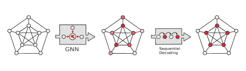
Figure 1: Illustration of the “Erdős goes neural” pipeline. First, a differentiable loss is derived for a given problem using the probabilistic method. Next, a GNN is trained in an unsupervised way using the derived loss to output a probability distribution over the nodes, essentially providing a probabilistic certificate for the existence of a low cost feasible solution. At inference time, a discrete solution satisfying the certificate is obtained in a sequential and deterministic manner by the method of conditional expectation.

2 Related work and background

2.1 Neural networks for combinatorial optimization

Most neural approaches to CO are supervised. One of the first modern neural networks were the Pointer Networks [75], which utilized a sequence-to-sequence model for the travelling salesman problem (TSP). Since then, numerous works have combined GNNs with various heuristics and search procedures to solve classical CO problems, such as quadratic assignment [54], graph matching [6], graph coloring [43], TSP [45, 35], and even sudoku puzzles [55]. Another fruitful direction has been the fusion with solvers. For example, Neurocore [62] incorporates an MLP to a SAT solver to enhance variable branching decisions, whereas Gasse et al. [27] learn branching approximations by a GNN and imitation learning. Further, Wang et al. [79] include an approximate SDP satisfiability solver as a neural network layer and Vlastelica et al. [77] incorporate exact solvers within a differentiable architecture by smoothly interpolating the solver’s piece-wise constant output. Unfortunately, the success of supervised approaches hinges on building large training sets with already solved hard instances, resulting in a chicken and egg situation. Moreover, since it is hard to efficiently sample unbiased and representative labeled instances of an NP-hard problem [87], labeled instance generation is likely not a viable long-term strategy either.

Training neural networks without labels is generally considered to be more challenging. One possibility is to use RL: Khalil et al. [38] combine Q-Learning with a greedy algorithm and structure2vec embeddings to solve max-cut, minimum vertex cover, and TSP. Q-Learning is also used in [7] for the maximum common subgraph problem. On the subject of TSP, the problem was also solved with policy gradient learning combined with attention [41, 20, 9]. Attention is ubiquitous in problems that deal with sequential data, which is why it has been widely used with RL for the problem of vehicle routing [25, 52, 56, 33]. Another interesting application of RL is the work of Yolcu and Poczos [88], where the REINFORCE algorithm is employed in order to learn local search heuristics for the SAT problem. This is combined with curriculum learning to improve stability during training. Finally, Chen and Tian [16] use actor-critic learning to iteratively improve complete solutions to combinatorial problems. Though a promising research direction, deep RL methods are far from ideal, as they can be sample inefficient and notoriously unstable to train—possibly due to poor gradient estimates, dependence on initial conditions, correlations present in the sequence of observations, bad rewards, sub-optimal hyperparameters, or poor exploration [69, 53, 31, 49].

The works that are more similar to ours are those that aim to train neural networks in a differentiable and end-to-end manner: Toenshoff et al. [70] model CO problems in terms of a constraint language and utilize a recurrent GNN, where all variables that coexist in a constraint can exchange messages. Their model is completely unsupervised and is suitable for problems that can be modeled as maximum constraint satisfaction problems. For other types of problems, like independent set, the model relies on empirically selected loss functions to solve the task. Amizadeh et al. [2, 3] train a GNN in an unsupervised manner to solve the circuit-SAT and SAT problems by minimizing an appropriate energy function. Finally, Yao et al. [86] train a GNN for the max-cut problem on regular graphs without supervision by optimizing a smooth relaxation of the cut objective and policy gradient.

Our approach innovates from previous works in the following ways: it enables training a neural network in an unsupervised, differentiable, and end-to-end manner, while also ensuring that identified solutions will be integral and will satisfy problem constraints. Crucially, this is achieved in a simple and mathematically-principled way, without resorting to continuous relaxations, regularization, or heuristic corrections of improper solutions. In addition, our approach does not necessitate polynomial-time reductions, but solves each problem directly.

2.2 Background: the probabilistic method

The probabilistic method is a nonconstructive proof method pioneered by Paul Erdős. It is used to demonstrate the existence of objects with desired combinatorial properties [1, 22, 68] but has also served as the foundation for important algorithms in the fields of computer science and combinatorial optimization [50, 58].

Let us consider the common didactic example of the maximum cut problem on a simple undirected graph [48]. The goal is to bipartition the nodes of the graph in such a way that the number of edges with endpoints in both partitions (i.e., the cardinality of the cut-set) is maximized. For simplicity we will refer to the cardinality of the cut-set as the cut. Suppose we decide the bipartition based on a fair coin flip, i.e., we split the nodes of the graph by assigning them to a heads or a tails set. An edge belongs to the cut-set when its endpoints belong to different sets. This happens with probability $\nicefrac{{1}}{{2}}$, which implies that the expected cut will be equal to half of the edges of the graph. Thus, by Markov’s inequality and given that the cut is non-negative, it follows that there exists a bipartitioning that contains at least half of the edges of the graph.

To obtain such a solution deterministically, we will utilize the method of conditional expectation [58]: we sequentially visit every node $v_{i}$ in the graph and we compute the expected cut conditioned on $v_{i}$ belonging to the heads or tails set (together with all the decisions made until the $i$-th step) and add $v_{i}$ to the set (heads or tails) that yields smaller conditional expected cut. Since the (conditional) expectation can only improve at every step, the sets recovered are guaranteed to cut at least half the edges of the graph, as proved earlier.

Our goal is to re-purpose this classic approach to tackle combinatorial optimization problems with deep learning. Instead of using a naive probability assignment like in the maxcut example, the probability distribution is learned by a GNN which allows us to obtain higher quality solutions. Additionally, we show how this argument may be extended to incorporate constraints within the learning paradigm.

3 The Erdős probabilistic method for deep learning

We focus on combinatorial problems on weighted graphs $G=(V,E,w)$ that are modelled as constrained optimization problems admitting solutions that are node sets:

$$\min_{S\subseteq V}\ f(S;G)\quad\text{subject to}\quad S\in\Omega.$$ (1)

Above, $\Omega$ is a family of sets having a desired property, such as forming a clique or covering all nodes. This yields a quite general formulation that can encompass numerous classical graph-theoretic problems, such as the maximum clique and minimum vertex cover problems.

3.1 The “Erdős Goes Neural” pipeline

Rather than attempting to optimize the non-differentiable problem (1) directly, we propose to train a GNN to identify distributions of solutions with provably advantageous properties. Our approach is inspired by Erdős’ probabilistic method, a well known technique in the field of combinatorics that is used to prove the existence of an object with a desired combinatorial property.

As visualized in Figure 1, our method consists of three steps:

1. Construct a GNN $g_{\theta}$ that outputs a distribution $\mathcal{D}=g_{\theta}(G)$ over sets.

2. Train $g_{\theta}$ to optimize the probability that there exists a valid $S^{*}\sim\mathcal{D}$ of small cost $f(S^{*};G)$.

3. Deterministically recover $S^{*}$ from $\mathcal{D}$ by the method of conditional expectation.

There are several possibilities in instantiating $\mathcal{D}$. We opt for the simplest and suppose that the decision of whether $v_{i}\in S$ is determined by a Bernoulli random variable $x_{i}$ of probability $p_{i}$. The network can trivially parametrize $\mathcal{D}$ by computing $p_{i}$ for every node $v_{i}$. Keeping the distribution simple will aid us later on to tractably control relevant probability estimates.

Next, we discuss how $g_{\theta}$ can be trained (Section 3.2) and how to recover $S^{*}$ from $\mathcal{D}$ (Section 3.3).

3.2 Deriving a probabilistic loss function

The main challenge of our method lies in determining how to tractably and differentiably train $g_{\theta}$. Recall that our goal is to identify a distribution that contains low-cost and valid solutions.

3.2.1 The probabilistic loss

Aiming to build intuition, let us first consider the unconstrained case. To train the network, we construct a loss function $\ell(\mathcal{D};G)$ that abides to the following property:

$$P(f(S;G)<\ell(\mathcal{D};G))>t\quad\text{with}\quad\mathcal{D}=g_{\theta}(G).$$ (2)

Any number of tail inequalities can be used to instantiate such a loss, depending on the structure of $f$. If we only assume that $f$ is non-negative, Markov’s inequality yields

$$\ell(\mathcal{D};G)\triangleq\frac{\mathbb{E}\left[f(S;G)\right]}{1-t}\quad\text{for any}\quad t\in[0,1).$$

If the expectation cannot be computed in closed-form, then any upper bound also suffices.

The main benefit of approaching the problem in this manner is that the surrogate (and possibly differentiable) loss function $\ell(\mathcal{D};G)$ can act as a certificate for the existence of a good set in the support of $\mathcal{D}$. To illustrate this, suppose that one has trained $g_{\theta}$ until the loss is sufficiently small, say $\ell(\mathcal{D};G)=\epsilon$. Then, by the probabilistic method, there exists with strictly positive probability a set $S^{*}$ in the support of $\mathcal{D}$ whose cost $f(S^{*};G)$ is at most $\epsilon$.

3.2.2 The probabilistic penalty loss

To incorporate constraints, we take inspiration from penalty methods in constrained optimization and add a term to the loss function that penalizes deviations from the constraint.

Specifically, we define the probabilistic penalty function $f_{p}(S;G)\triangleq f(S;G)+\bm{1}_{S\notin\Omega}\,\beta,$ where $\beta$ is a scalar. The expectation of $f_{p}$ yields the probabilistic penalty loss:

$$\ell(\mathcal{D},G)\triangleq\mathbb{E}\left[f(S;G)\right]+P(S\notin\Omega)\,\beta.$$ (3)

We prove the following:

Theorem 1.

Fix any $\beta>\max_{S}f(S;G)$ and let $\ell(\mathcal{D},G)=(1-t)\epsilon<\beta$. With probability at least $t$, set $S^{*}\sim\mathcal{D}$ satisfies

$$f(S^{*};G)<\ell(\mathcal{D};G)/(1-t)\ \ \text{and}\ \ S^{*}\in\Omega,$$

under the condition that $f$ is non-negative.

Hence, similar to the unconstrained case, the penalized loss acts as a certificate for the existence of a low-cost set, but now the set is also guaranteed to abide to the constraints $\Omega$. The main requirement for incorporating constraints is to be able to differentiably compute an upper estimate of the probability $P(S\notin\Omega)$. A worked out example of how $P(S\notin\Omega)$ can be controlled is provided in Section 4.1.

3.2.3 The special case of linear box constraints

An alternative construction can be utilized when problem (1) takes the following form:

$$\min_{S\subseteq V}\ f(S;G)\quad\text{subject to}\quad\sum_{v_{i}\in S}a_{i}\in[b_{l},b_{h}],$$ (4)

with $a_{i}$, $b_{l}$, and $b_{h}$ being non-negative scalars.

We tackle such instances with a two-step approach. Denote by $\mathcal{D}^{0}$ the distribution of sets predicted by the neural network and let $p_{1}^{0},\ldots,p_{n}^{0}$ be the probabilities that parametrize it. We rescale these probabilities such that the constraint is satisfied in expectation:

$$\sum_{v_{i}\in V}a_{i}p_{i}=\frac{b_{l}+b_{h}}{2},\quad\text{where}\quad p_{i}=\text{clamp}{\left(c\,p_{i}^{0},0,1\right)}\quad\text{and}\quad c\in\mathbb{R}.$$

Though non-linear, the aforementioned feasible re-scaling can be carried out by a simple iterative scheme (detailed in Section D.2). If we then proceed as in Section 3.2.1 by utilizing a probabilistic loss function that guarantees the existence of a good unconstrained solution, we have:

Theorem 2.

Let $\mathcal{D}$ be the distribution obtained after successful re-scaling of the probabilities. For any (unconstrained) probabilistic loss function that abides to $P(f(S;G)<\ell(\mathcal{D};G))>t$, set $S^{*}\sim\mathcal{D}$ satisfies $f(S^{*};G)<\ell(\mathcal{D};G)\ \text{and}\ \sum_{v_{i}\in S^{*}}a_{i}\in[b_{l},b_{h}],$ with probability at least $t-2\exp{\left(-(b_{h}-b_{l})^{2}/\sum_{i}2a_{i}^{2}\right)}$.

Section 4.2 presents a worked-out example of how Theorem 2 can be applied.

3.3 Retrieving integral solutions

A simple way to retrieve a low cost integral solution $S^{*}$ from the learned distribution $\mathcal{D}$ is by monte-carlo sampling. Then, if $S^{*}\sim\mathcal{D}$ with probability $t$, the set can be found within the first $k$ samples with probability at least $1-(1-t)^{k}$. However, our goal is to deterministically obtain $S^{*}$ so we will utilize the method of conditional expectation that was introduced in Section 2.2.

Let us first consider the unconstrained case. Given $\mathcal{D}$, the goal is to identify a set $S^{*}$ that satisfies $f(S^{*};G)\leq\mathbb{E}\left[f(S;G)\right]$. To achieve this, one starts by sorting $v_{1},\ldots,v_{n}$ in order of decreasing probabilities $p_{i}$. Let $S_{\text{reject}}=\varnothing$ be the set of nodes not accepted in the solution. Set $S^{*}=\varnothing$ is then iteratively updated one node at a time, with $v_{i}$ being included to $S^{*}$ in the $i$-th step if $\mathbb{E}\left[f(S;G)\ |\ S^{*}\subset S,\ S\cap S_{\text{reject}}=\varnothing,\ \text{ and }v_{i}\in S\right]<\mathbb{E}\left[f(S;G)\ |\ S^{*}\subset S,\ S\cap S_{\text{reject}}=\varnothing,\ \text{ and }v_{i}\notin S\right]$. This sequential decoding works because the conditional expectation never increases.

In the case of the probabilistic penalty loss, the same procedure is applied w.r.t. the expectation of $f_{p}(S;G)$. The latter ensures that the decoded set will match the claims of Theorem 1. For the method of Section 3.2.3, a sequential decoding can guarantee either that the cost of $f(S^{*};G)$ is small or that the constraint is satisfied.

4 Case studies

This section demonstrates how our method can be applied to two well known NP-hard problems: the maximum clique [12] and the constrained minimum cut [15] problems.

4.1 The maximum clique problem

A clique is a set of nodes such that every two distinct nodes are adjacent. The maximum clique problem entails identifying the clique of a given graph with the largest possible number of nodes:

$$\min_{S\subseteq V}-w(S)\quad\text{subject to}\quad S\in\Omega_{\text{clique}},$$ (5)

with $\Omega_{\textit{clique}}$ being the family of cliques of graph $G$ and $w(S)=\sum_{v_{i},v_{j}\in S}w_{ij}$ being the weight of $S$. Optimizing $w(S)$ is a generalization of the standard cardinality formulation to weighted graphs. For simple graphs, both weight and cardinality formulations yield the same minimum.

We can directly apply the ideas of Section 3.2.2 to derive a probabilistic penalty loss:

Corollary 1.

Fix positive constants $\gamma$ and $\beta$ satisfying $\max_{S}w(S)\leq\gamma\leq\beta$ and let $w_{ij}\leq 1$. If

$$\ell_{\text{clique}}(\mathcal{D},G) \triangleq\gamma-(\beta+1)\sum_{(v_{i},v_{j})\in E}w_{ij}p_{i}p_{j}+\frac{\beta}{2}\sum_{v_{i}\neq v_{j}}p_{i}p_{j}\leq\epsilon(1-t)$$

then, with probability at least $t$, set $S^{*}\sim\mathcal{D}$ is a clique of weight $w(S^{*})>\gamma-\epsilon$.

The loss function $\ell_{\text{clique}}$ can be evaluated in linear time w.r.t. the number of edges of $G$ by rewriting the rightmost term as $\sum_{v_{i}\neq v_{j}}p_{i}p_{j}=(\sum_{v_{i}\in V}p_{i})^{2}-\sum_{(v_{i},v_{j})\in E}2p_{i}p_{j}$.

A remark. One may be tempted to fix $\beta\to\infty$, such that the loss does not feature any hyper-parameters. However, with mini-batch gradient descent it can be beneficial to tune the contribution of the two terms in the loss to improve the optimization. This was also confirmed in our experiments, where we selected the relative weighting according to a validation set.

Decoding cliques.

After the network is trained, valid solutions can be decoded sequentially based on the procedure of Section 3.3. The computation can also be sped up by replacing conditional expectation evaluations (one for each node) by a suitable upper bound. Since the clique property is maintained at every point, we can also efficiently decode cliques by sweeping nodes (in the order of larger to smaller probability) and only adding them to the set when the clique constraint is satisfied.

4.2 Graph partitioning

The simplest partitioning problem is the minimum cut: find set $S\subset V$ such that $\text{cut}\left(S\right)=\sum_{v_{i}\in S,\ v_{j}\notin{S}}w_{ij}$ is minimized. Harder variants of partitioning aim to provide control on partition balance, as well as cut weight. We consider the following constrained min-cut problem:

$$\underset{S}{\min}\ \text{cut}\left(S\right)\quad\text{subject to}\quad\text{vol}\left(S\right)\in[v_{l},v_{h}],$$

where the volume $\text{vol}\left(S\right)=\sum_{v_{i}\in S}d_{i}$ of a set is the sum of the degrees of its nodes.

The above can be shown to be NP-hard [32] and exhibits strong connections with other classical formulations: it is a volume-balanced graph partitioning problem [5] and can be used to minimize graph conductance [18] by scanning through solutions in different volume intervals and selecting the one whose cut-over-volume ratio is the smallest (this is how we test it in Section 5).

We employ the method described in Section 3.2.3 to derive a probabilistic loss function:

Corollary 2.

Let the probabilities $p_{1},\ldots,p_{n}$ giving rise to $\mathcal{D}$ be re-scaled such that $\sum_{v_{i}\in V}d_{i}p_{i}=\frac{v_{l}+v_{h}}{2}$ and, further, fix $\ell_{\text{cut}}(\mathcal{D};G)\triangleq\sum_{v_{i}\in V}d_{i}p_{i}-2\sum_{(v_{i},v_{j})\in E}p_{i}p_{j}w_{ij}.$ Set $S^{*}\sim\mathcal{D}$ satisfies

$$\text{cut}\left(S^{*}\right)<{\ell_{\text{cut}}(\mathcal{D};G)}/{(1-t)}\quad\text{and}\quad\text{vol}\left(S^{*}\right)\in[v_{l},v_{h}],$$

with probability at least $t-2\exp{\left(-(v_{h}-v_{l})^{2}/\sum_{i}2d_{i}^{2}\right)}$.

The derived loss function $\ell_{\text{cut}}$ can be computed efficiently on a sparse graph, as its computational complexity is linear on the number of edges.

Decoding clusters.

Retrieving a set that respects Corollary 2 can be done by sampling. Alternatively, the method described in Section 3.3 can guarantee that the identified cut is at most as small as the one certified by the probabilistic loss. In the latter case, the linear box constraint can be practically enforced by terminating before the volume constraint gets violated.

5 Empirical evaluation

We evaluate our approach in its ability to find large cliques and partitions of good conductance.

5.1 Methods

We refer to our network as Erdős’ GNN, paying tribute to the pioneer of the probabilistic method that it is inspired from. Its architecture comprises of multiple layers of the Graph Isomorphism Network (GIN) [82] and a Graph Attention (GAT) [74] layer. Furthermore, each convolution layer was equipped with skip connections, batch normalization and graph size normalization [21]. In addition to a graph, we gave our network access to a one-hot encoding of a randomly selected node, which encourages locality of solutions, allows for a trade-off between performance and efficiency (by rerunning the network with different samples), and helps the network break symmetries [64]. Our network was trained with mini-batch gradient descent, using the Adam optimizer [40] and was implemented on top of the pytorch geometric API [23].

Maximum clique. We compared against three neural networks, three discrete algorithms, and two integer-programming solvers: The neural approaches comprised of RUN-CSP, Bomze GNN, and MS GNN. The former is a SotA unsupervised network incorporating a reduction to independent set and a post-processing of invalid solutions with a greedy heuristic. The latter two, though identical in construction to Erdős’ GNN, were trained based on standard smooth relaxations of the maximum clique problem with a flat 0.5-threshold discretization [51, 11]. Since all these methods can produce multiple outputs for the same graph (by rerunning them with different random node attributes), we fix two time budgets for RUN-CSP and Erdős’ GNN, that we refer to as “fast" and “accurate" and rerun them until the budget is met (excluding reduction costs). On the other hand, the Bomze and MS GNNs are rerun 25 times, since further repetitions did not yield relevant improvements. We considered the following algorithms: the standard Greedy MIS Heur. which greedily constructs a maximal independent set on the complement graph, NX MIS approx. [13], and Toenshoff-Greedy [70]. Finally, we formulated the maximum clique in integer form [12] and solved it with CBC [34] and Gurobi 9.0 [29], an open-source solver provided with Google’s OR-Tools package and a SotA commercial solver. We should stress that our evaluation does not intend to establish SotA results (which would require a more exhaustive comparison), but aims to comparatively study the weaknesses and strengths of key unsupervised approaches.

Local partitioning. We compared against two neural networks and four discrete algorithms. To the extent of our knowledge, no neural approach for constrained partitioning exists in the literature. Akin to maximum clique, we built the L1 GNN and L2 GNN to be identical to Erdős’ GNN and trained them based on standard smooth $\ell_{1}$ and $\ell_{2}$ relaxations of the cut combined with a volume penalty. On the other hand, a number of algorithms are known for finding small-volume sets of good conductance. We compare to well-known and advanced algorithms [24]: Pagerank-Nibble [4], Capacity Releasing Diffusion (CRD) [78], Max-flow Quotient-cut Improvement (MQI) [42] and Simple-Local [73].

5.2 Data

Experiments for the maximum clique were conducted in the IMDB, COLLAB [37, 85] and TWITTER [44] datasets, listed in terms of increasing graph size. Further experiments were done on graphs generated from the RB model [81], that has been specifically designed to generate challenging problem instances. We worked with three RB datasets: a training set containing graphs of up to 500 nodes [70], a newly generated test set containing graphs of similar size, and a set of instances that are up to 3 times larger [80, 45, 70]. On the other hand, to evaluate partitioning, we focused on the FACEBOOK [71], TWITTER, and SF-295 [84] datasets, with the first being a known difficult benchmark. More details can be found in the Appendix.

Evaluation. We used a 60-20-20 split between training, validation, and test for all datasets, except for the RB model data (details in paragraph above). Our baselines often require the reduction of maximum clique to independent set, which we have done when necessary. The reported time costs factor in the cost of reduction. During evaluation, for each graph, we sampled multiple inputs, obtained their solutions, and kept the best one. This was repeated for all neural approaches and local graph clustering algorithms. Solvers were run with multiple time budgets.

	IMDB	COLLAB	TWITTER
Erdős’ GNN (fast)	1.000 (0.08 s/g)	0.982 $\pm$ 0.063 (0.10 s/g)	0.924 $\pm$ 0.133 (0.17 s/g)
Erdős’ GNN (accurate)	1.000 (0.10 s/g)	0.990 $\pm$ 0.042 (0.15 s/g)	0.942 $\pm$ 0.111 (0.42 s/g)
RUN-CSP (fast)	0.823 $\pm$ 0.191 (0.11 s/g)	0.912 $\pm$ 0.188 (0.14 s/g)	0.909 $\pm$ 0.145 (0.21 s/g)
RUN-CSP (accurate)	0.957 $\pm$ 0.089 (0.12 s/g)	0.987 $\pm$ 0.074 (0.19 s/g)	0.987 $\pm$ 0.063 (0.39 s/g)
Bomze GNN	0.996 $\pm$ 0.016 (0.02 s/g)	0.984 $\pm$ 0.053 (0.03 s/g)	0.785 $\pm$ 0.163 (0.07 s/g)
MS GNN	0.995 $\pm$ 0.068 (0.03 s/g)	0.938 $\pm$ 0.171 (0.03 s/g)	0.805 $\pm$ 0.108 (0.07 s/g)
NX MIS approx.	0.950 $\pm$ 0.071 (0.01 s/g)	0.946 $\pm$ 0.078 (1.22 s/g)	0.849 $\pm$ 0.097 (0.44 s/g)
Greedy MIS Heur.	0.878 $\pm$ 0.174 (1e-3 s/g)	0.771 $\pm$ 0.291 (0.04 s/g)	0.500 $\pm$ 0.258 (0.05 s/g)
Toenshoff-Greedy	0.987 $\pm$ 0.050 (1e-3 s/g)	0.969 $\pm$ 0.087 (0.06 s/g)	0.917 $\pm$ 0.126 (0.08 s/g)
CBC (1s)	0.985 $\pm$ 0.121 (0.03 s/g)	0.658 $\pm$ 0.474 (0.49 s/g)	0.107 $\pm$ 0.309 (1.48 s/g)
CBC (5s)	1.000 (0.03 s/g)	0.841 $\pm$ 0.365 (1.11 s/g)	0.198 $\pm$ 0.399 (4.77 s/g)
Gurobi 9.0 (0.1s)	1.000 (1e-3 s/g)	0.982 $\pm$ 0.101 (0.05 s/g)	0.803 $\pm$ 0.258 (0.21 s/g)
Gurobi 9.0 (0.5s)	1.000 (1e-3 s/g)	0.997 $\pm$ 0.035 (0.06 s/g)	0.996 $\pm$ 0.019 (0.34 s/g)
Gurobi 9.0 (1s)	1.000 (1e-3 s/g)	0.999 $\pm$ 0.015 (0.06 s/g)	1.000 (0.34 s/g)
Gurobi 9.0 (5s)	1.000 (1e-3 s/g)	1.000 (0.06 s/g)	1.000 (0.35 s/g)

Table 1: Test set approximation ratios for all methods on real-world datasets. For solvers, time budgets are listed next to the name. Pareto-optimal solutions are indicated in bold, whereas italics indicate constraint violation (we report the results only for correctly solved instances).

5.3 Results: maximum clique

Table 1 reports the test set approximation ratio, i.e., the ratio of each solution’s cost over the optimal cost. For simple datasets, such as IMDB, most neural networks achieve similar performance and do not violate the problem constraints. On the other hand, the benefit of the probabilistic penalty method becomes clear on the more-challenging Twitter dataset, where training with smooth relaxation losses yields significantly worse results and constraint violation in at least 78% of the instances (see Appendix). Erdős’ GNN always respected constraints. Our method was also competitive w.r.t. network RUN-CSP and the best solver, consistently giving better results when optimizing for speed (“fast"). The most accurate method overall was Gurobi, which impressively solved all instances perfectly given sufficient time. As observed, Gurobi has been heavily engineered to provide significant speed up w.r.t. CBC. Nevertheless, we should stress that both solvers scale poorly with the number of nodes and are not viable candidates for graphs with more than a few thousand nodes.

Table 2 tests the best methods on hard instances. We only provide the results for Toenshoff-Greedy, RUN-CSP, and Gurobi, as the other baselines did not yield meaningful results. Erdős’ GNN can be seen to be better than RUN-CSP in the training and test set and worse for larger, out of distribution, instances. However, both neural approaches fall behind the greedy algorithm and Gurobi, especially when optimizing for quality. The performance gap is pronounced for small instances but drops significantly for larger graphs, due to Gurobi’s high computational complexity. It is also interesting to observe that the neural approaches do better on the training set than on the test set. Since both neural methods are completely unsupervised, the training set performance can be taken at face value (the methods never saw any labels). Nevertheless, the results also show that both methods partially overfit the training distribution. The main weakness of Erdős’ GNN is that its performance degrades when testing it in larger problem instances. Nevertheless, it is encouraging to observe that even on graphs of at most 1500 nodes, both our “fast” method and RUN-CSP surpass Gurobi when given the same time-budget. We hypothesize that this phenomenon will be more pronounced with larger graphs.

	Training set	Test set	Large Instances
Erdős’ GNN (fast)	0.899 $\pm$ 0.064 (0.27 s/g)	0.788 $\pm$ 0.065 (0.23 s/g)	0.708 $\pm$ 0.027 (1.58 s/g)
Erdős’ GNN (accurate)	0.915 $\pm$ 0.060 (0.53 s/g)	0.799 $\pm$ 0.067 (0.46 s/g)	0.735 $\pm$ 0.021 (6.68 s/g)
RUN-CSP (fast)	0.833 $\pm$ 0.079 (0.27 s/g)	0.738 $\pm$ 0.067 (0.23 s/g)	0.771 $\pm$ 0.032 (1.84 s/g)
RUN-CSP (accurate)	0.892 $\pm$ 0.064 (0.51 s/g)	0.789 $\pm$ 0.053 (0.47 s/g)	0.804 $\pm$ 0.024 (5.46 s/g)
Toenshoff-Greedy	0.924 $\pm$ 0.060 (0.02 s/g)	0.816 $\pm$ 0.064 (0.02 s/g)	0.829 $\pm$ 0.027 (0.35 s/g)
Gurobi 9.0 (0.1s)	0.889 $\pm$ 0.121 (0.18 s/g)	0.795 $\pm$ 0.118 (0.16 s/g)	0.697 $\pm$ 0.033 (1.17 s/g)
Gurobi 9.0 (0.5s)	0.962 $\pm$ 0.076 (0.34 s/g)	0.855 $\pm$ 0.083 (0.31 s/g)	0.697 $\pm$ 0.033 (1.54 s/g)
Gurobi 9.0 (1.0s)	0.980 $\pm$ 0.054 (0.45 s/g)	0.872 $\pm$ 0.070 (0.40 s/g)	0.705 $\pm$ 0.039 (2.05 s/g)
Gurobi 9.0 (5.0s)	0.998 $\pm$ 0.010 (0.76 s/g)	0.884 $\pm$ 0.062 (0.68 s/g)	0.790 $\pm$ 0.285 (6.01 s/g)
Gurobi 9.0 (20.0s)	0.999 $\pm$ 0.003 (1.04 s/g)	0.885 $\pm$ 0.063 (0.96 s/g)	0.807 $\pm$ 0.134 (21.24 s/g)

Table 2: Hard maximum clique instances (RB). We report the approximation ratio (bigger is better) in the training and test set, whereas the rightmost column focuses on a different distribution consisting of graphs of different sizes. Execution time is measured in sec. per graph (s/g). Pareto-optimal solutions are in bold.

5.4 Results: local graph partitioning

The results of all methods and datasets are presented in Table 3. To compare fairly with previous works, we evaluate partitioning quality based on the measure of local conductance, $\phi(S)=\text{cut}\left(S\right)/\text{vol}\left(S\right)$, even though our method only indirectly optimizes conductance. Nevertheless, Erdős’ GNN outperforms all previous algorithms by a considerable margin. We would like to stress that this result is not due to poor usage of previous methods: we rely on a well-known implementation [24] and select the parameters of all non-neural baselines by grid-search on a held-out validation set. We also do not report performance when a method (Pagerank-Nibble) returns the full graph as a solution [78].

It is also interesting to observe that, whereas all neural approaches perform well, GNN trained with a probabilistic loss attains better conductance across all datasets. We remind the reader that all three GNNs feature identical architectures and that the L1 and L2 loss functions are smooth relaxations that are heavily utilized in partitioning problems [14]. Furthermore, due to its high computational complexity and the extra overhead that is incurred when constructing the problem instances for large graphs, Gurobi performed poorly in all but the smallest graphs.We argue that the superior solution quality of Erdős’ GNN serves as evidence for the benefit of our unsupervised framework.

	SF-295	FACEBOOK	TWITTER
Erdős’ GNN	0.124 $\pm$ 0.001 (0.22 s/g)	0.156 $\pm$ 0.026 (289.28 s/g)	0.292 $\pm$ 0.009 (6.17 s/g)
L1 GNN	0.188 $\pm$ 0.045 (0.02 s/g)	0.571 $\pm$ 0.191 (13.83 s/g)	0.318 $\pm$ 0.077 (0.53 s/g)
L2 GNN	0.149 $\pm$ 0.038 (0.02 s/g)	0.305 $\pm$ 0.082 (13.83 s/g)	0.388 $\pm$ 0.074 (0.53 s/g)
Pagerank-Nibble	0.375 $\pm$ 0.001 (1.48 s/g)	N/A	0.603 $\pm$ 0.005 (20.62 s/g)
CRD	0.364 $\pm$ 0.001 (0.03 s/g)	0.301 $\pm$ 0.097 (596.46 s/g)	0.502 $\pm$ 0.020 (20.35 s/g)
MQI	0.659 $\pm$ 0.000 (0.03 s/g)	0.935 $\pm$ 0.024 (408.52 s/g)	0.887 $\pm$ 0.007 (0.71 s/g)
Simple-Local	0.650 $\pm$ 0.024 (0.05 s/g)	0.955 $\pm$ 0.019 (404.67 s/g)	0.895 $\pm$ 0.008 (0.84 s/g)
Gurobi (10s)	0.105 $\pm$ 0.000 (0.16 s/g)	0.961 $\pm$ 0.010 (1787.79 s/g)	0.535 $\pm$ 0.006 (52.98 s/g)

Table 3: Cluster conductance on the test set (smaller is better) and execution time measured in sec. per graph. Pareto-optimal solutions are in bold.

6 Conclusion

We have presented a mathematically principled framework for solving constrained combinatorial problems on graphs that utilizes a probabilistic argument to guarantee the quality of its solutions. As future work, we would like to explore different avenues in which the sequential decoding could be accelerated. We aim to expand the ability of our framework to incorporate different types of constraints. Though we can currently support constraints where node order is not necessarily important (e.g., clique, cover, independent set), we would like to determine whether it is possible to handle more complex constraints, e.g., relating to trees or paths [19]. Overall, we believe that this work presents an important step towards solving CO problems in an unsupervised way and opens up the possibility of further utilizing techniques from combinatorics and the theory of algorithms in the field of deep learning.

7 Broader impact

This subfield of deep learning that our work belongs to is still in its nascent stages, compared to others like computer vision or translation. Therefore, we believe that it poses no immediate ethical or societal challenges. However, advances in combinatorial optimization through deep learning can have significant long term consequences. Combinatorial optimization tasks are important in manufacturing and transportation. The ability to automate these tasks will likely lead to significant improvements in productivity and efficiency in those sectors which will affect many aspects of everyday life. On the other hand, these tasks would be otherwise performed by humans which means that such progress may eventually lead to worker displacement in several industries. Combinatorial optimization may also lead to innovations in medicine and chemistry, which will be beneficial to society in most cases.

Our work follows the paradigm of unsupervised learning which means that it enjoys some advantages over its supervised counterparts. The lack of labeled instances implies a lack of label bias. Consequently, we believe that unsupervised learning has the potential to avoid many of the issues (fairness, neutrality) that one is faced with when dealing with labeled datasets. That does not eliminate all sources of bias in the learning pipeline, but it is nonetheless a step towards the right direction.

Finally, we acknowledge that combinatorial optimization has also been widely applied in military operations. However, even though this is not the intention of many researchers, we believe that it is just a natural consequence of the generality and universality of the problems in this field. Therefore, as with many technological innovations, we expect that the positives will outweigh the negatives as long as the research community maintains a critical outlook on the subject. Currently, the state of the field does not warrant any serious concerns and thus we remain cautiously optimistic about its impact in the world.

Appendix A Visual demonstration

Figure 2 provides a visual demonstration of the input and output of Erdős’ GNN in a simple instance of the maximum clique problem.

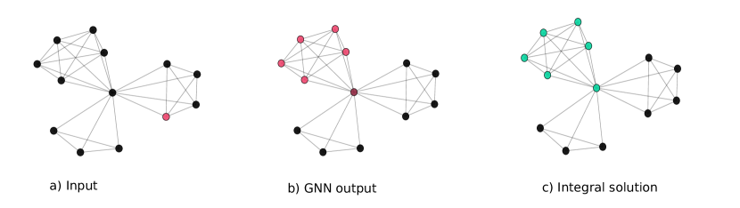
Figure 2: Illustration of our approach in a toy instance of the maximum clique problem from the IMDB dataset. a) A random node is selected to act as a ‘seed’. b) Erdős’ GNN outputs a probability distribution over the nodes (color intensity represents the probability magnitude) by exploring the graph in the vicinity of the seed. c) A set is sequentially decoded by starting from the node whose probability is the largest and iterating with the method of conditional expectation. The identified solution is guaranteed to obey the problem constraints, i.e., to be a clique.

We would like to make two observations. The first has to do with the role of the starting seed in the probability assignment produced by the network. In the maximum clique problem, we did not require the starting seed to be included in the solutions. This allowed the network to flexibly detect maximum cliques within its receptive field without being overly constrained by the random seed selection. This is illustrated in the example provided in the figure, where the seed is located inside a smaller clique and yet the network is able to produce probabilities that focus on the largest clique. On the other hand, in the local graph partitioning problem we forced the seed to always lie in the identified solution—this was done to ensure a fair comparison with previous methods. Our second observation has to do with the sequential decoding process. It is encouraging to notice that, even though the central hub node has a considerably lower probability than the rest of the nodes in the maximum clique, the method of conditional expectation was able to reliably decode the full maximum clique.

Appendix B Experimental details

B.1 Datasets

The following table presents key statistics of the datasets that were used in this study:

	IMDB	COLLAB	TWITTER	RB (Train)	RB (Test)	RB (Large Inst.)	SF-295	FACEBOOK
nodes	19.77	74.49	131.76	216.673	217.44	1013.25	26.06	7252.71
edges	96.53	2457.78	1709.33	22852	22828	509988.2	28.08	276411.19
reduction time	0.0003	0.006	0.024	0.018	0.018	0.252	–	–
number of test graphs	200	1000	196	2000	500	40	8055	14

Table 4: Average number of nodes and edges for the considered datasets. Reduction time corresponds to the average number of seconds needed to reduce a maximum clique instance to a maximum independent instance. Number of test graphs refers to the number of graphs that the methods were evaluated on, in a given dataset.

To speed up computation and training, for the Facebook dataset, we kept graphs consisting of at most 15000 nodes (i.e., 70 out of the total 100 available graphs of the dataset).

The RB test set can be downloaded from the following link: https://www.dropbox.com/s/9bdq1y69dw1q77q/cliques_test_set_solved.p?dl=0. The latter was generated using the procedure described by Xu [80]. We used a python implementation by Toenshoff et al. [70] that is available on the RUN-CSP repository: https://github.com/RUNCSP/RUN-CSP/blob/master/generate_xu_instances.py. Since the parameters of the original training set were not available, we selected a set of initial parameters such that the generated dataset resembles the original training set. As seen in Table 4, the properties of the generated test set are close to those of the training set. Specifically, the training set contained graphs whose size varied between 50 and 500 nodes and featured cliques of size 5 to 25. The test set was made out of graphs whose size was between 50 and 475 nodes and contained cliques of size 10 to 25. These minor differences provide a possible explanation for the drop in test performance of all methods (larger cliques tend to be harder to find).

All other datasets are publicly available.

B.2 Neural network architecture

In both problems, Erdős’ GNN and our own neural baselines were given as node features a one-hot encoding of a random node from the input graph. For the local graph partitioning setting, our networks consisted of 6 GIN layers followed by a multi-head GAT layer. The depth was kept constant across all datasets. We employed skip connections and batch-normalization at every layer. For the maximum clique problem, we also incorporated graph size normalization for each convolution, as we found that it improved optimization stability. The networks in this setting did not use a GAT layer, as we found that multi-head GAT had a negative impact on the speed/memory of the network, while providing only negligible benefits in accuracy. Furthermore, locality was enforced after each layer by masking the receptive field. That is, after 1 layer of convolution only 1-hop neighbors were allowed to have nonzero values, after 2 layers only 2-hop neighbors could have nonzero values, etc. The output of the final GNN layer was passed through a two layer perceptron giving as output one value per node. The aforementioned numbers were re-scaled to lie in $[0,1]$ (using a graph-wide min-max normalization) and were interpreted as probabilities $p_{1},\ldots,p_{n}$. In the case of local graph partitioning, the forward-pass was concluded by the appropriate re-scaling of the probabilities (as described in Section 3.2.3).

B.3 Local graph partitioning setup

Following the convention of local graph clustering algorithms, for each graph in the test set we randomly selected $d$ nodes of the input graph to act as cluster seeds, where $d=10,30$, and $100$ for SF-295, TWITTER, and FACEBOOK, respectively. Each method was run once for each seed resulting in $d$ sets per graph. We obtained one number per seed by averaging the conductances of the graphs. Table 3 reports the mean and standard deviation of these numbers. The correct procedure is the one described here.

The volume-constrained graph partitioning formulation can be used to minimize conductance as follows: Perform grid search over the range of feasible volumes and create a small interval around each target volume. Then, solve a volume-constrained partitioning problem for each interval, and return the set of smallest conductance identified.

We used a fast and randomized variant of the above procedure with all neural approaches and Gurobi (see Section C.2 for more details). Specifically, for each seed node we generated a random volume interval within the receptive field of the network, and solved the corresponding constrained partitioning problem. Our construction ensured that the returned sets always contained the seed node and had a controlled volume. For L1 and L2 GNN, we obtained the set by sampling from the output distribution. We drew 10 samples and kept the best. We found that in contrast to flat thresholding (like in the maximum clique), sampling yielded better results in this case.

For the parameter search of local graph clustering methods, we found the best performing parameters on a validation set via grid search when that was appropriate. For CRD, we searched for all the integer values in the [1,20] interval for all 3 of the main parameters of the algorithm. For Simple Local, we searched in the [0,1] interval for the locality parameter. Finally, for Pagerank-Nibble we set a lower bound on the volume that is 10 % of the total graph volume. It should be noted, that while local graph clustering methods achieved inferior conductance results, they do not require explicit specification of a receptive field which renders them more flexible.

B.4 Hardware and software

All methods were run on an Intel Xeon Silver 4114 CPU, with 192GB of available RAM. The neural networks were executed on a single RTX TITAN 25GB graphics card. The code was executed on version 1.1.0 of PyTorch and version 1.2.0 of PyTorch Geometric.

Appendix C Additional results

C.1 Maximum clique problem

The following experiments provide evidence that both the learning and decoding phases of our framework are important in obtaining valid cliques of large size.

C.1.1 Constraint violation

Table 5 reports the percentage of instances in which the clique constraint was violated in our experiments. Neural baselines optimized according to penalized continuous relaxations struggle to detect cliques in the COLLAB and TWITTER datasets, whereas Erdős’ GNN always respected the constraint.

	IMDB	COLLAB	TWITTER	RB (all datasets)
Erdős’ GNN (fast)	0%	0%	0%	0%
Erdős’ GNN (accurate)	0%	0%	0%	0%
Bomze GNN	0%	11.8%	78.1%	–
MS GNN	1%	15.1%	84.7%	–

Table 5: Percentage of test instances where the clique constraint was violated.

Thus, decoding solutions by the method of conditional expectation is crucial to ensure that the clique constraint is always satisfied.

C.1.2 Importance of learning

We also tested the efficacy of the learned probability distributions produced by our GNN on the Twitter dataset. We sampled multiple random seeds and produced the corresponding probability assignments by feeding the inputs to the GNN. These were then decoded with the method of conditional expectation and the best solution was kept. To measure the contribution of the GNN, we compared to random uniform probability assignments on the nodes. In that case, instead of multiple random seeds, we had the same number of multiple random uniform probability assignments. Again, these were decoded with the method of conditional expectation and the best solution was kept. The results of the experiment can be found in Table 6.

	Erdős’ GNN	U $\sim$ [0,1]
1 sample	0.821 $\pm$ 0.222	0.513 $\pm$ 0.266
3 samples	0.875 $\pm$ 0.170	0.694 $\pm$ 0.210
5 samples	0.905 $\pm$ 0.139	0.760 $\pm$ 0.172

Table 6: Approximation ratios with sequential decoding using the method of conditional expectation on the twitter dataset. The second column represents decoding with the probabilities produced by the GNN. The third column shows the results achieved by decoding random uniform probability assignments on the nodes.

As observed, the cliques identified by the trained GNN were significantly larger than those obtained when decoding a clique from a random probability assignment.

C.2 Local graph partitioning

We also attempted to find sets of small conductance using Gurobi. To ensure a fair comparison, we mimicked the setting of Erdős’ GNN and re-run the solver with three different time-budgets, making sure that the largest budget exceeded our method’s running time by approximately one order of magnitude. We used the following integer-programming formulation of the constrained graph partitioning problem:

$$\min_{x_{1},\ldots,x_{n}\in\{0,1\}} \sum_{(v_{i},v_{j})\in E}(x_{i}-x_{j})^{2}$$ (6)

subject to $$\quad\left(1-\frac{1}{4}\right)\,\text{vol}\leq\sum_{v_{i}\in V}x_{i}d_{i}\leq\left(1+\frac{1}{4}\right)\,\text{vol}\quad\text{and}\quad x_{s}=1.$$

Above, vol is a target volume and $s$ is the index of the seed node (see explanation in Section B.3). Each binary variable $x_{i}$ is used to indicate membership in the solution set. In order to encourage local solutions on a global solver like Gurobi, the generated target volumes were set to lie in an interval that is attainable within a fixed receptive field (identically to the neural baselines). Additionally, the seed node $v_{s}$ was also required to be included in the solution. The above choices are consistent with the neural baselines and the local graph partitioning setting.

The results are shown in Table 7. Due to its high computational complexity, Gurobi performed poorly in all but the smallest instances. In the FACEBOOK dataset, which contains graphs of 7k nodes on average, Erdős’ GNN was impressively able to find sets of more than 6$\times$ smaller conductance, while also being 6$\times$ faster.

	SF-295	FACEBOOK	TWITTER
Gurobi (0.1s)	0.107 $\pm$ 0.000 (0.16 s/g)	0.972 $\pm$ 0.000 (799.508 s/g)	0.617 $\pm$ 0.012 (3.88 s/g)
Gurobi (1s)	0.106 $\pm$ 0.000 (0.16 s/g)	0.972 $\pm$ 0.000 (893.907 s/g)	0.544 $\pm$ 0.007 (12.41 s/g)
Gurobi (10s)	0.105 $\pm$ 0.000 (0.16 s/g)	0.961 $\pm$ 0.010 (1787.79 s/g)	0.535 $\pm$ 0.006 (52.98 s/g)
Erdős’ GNN	0.124 $\pm$ 0.001 (0.22 s/g)	0.156 $\pm$ 0.026 (289.28 s/g)	0.292 $\pm$ 0.009 (6.17 s/g)

Table 7: Average conductance of sets identified by Gurobi and Erdős’ GNN (these results are supplementary to those of Table 3).

It should be noted that the time budget allowed for Gurobi only pertains to the optimization time spent (for every seed). There are additional costs in constructing the problem instances and their constraints for each graph. These costs become particularly pronounced in larger graphs, where setting up the problem instance takes more time than the allocated optimization budget. We report the total time cost in seconds per graph (s/g).

Appendix D Deferred technical arguments

D.1 Proof of Theorem 1

In the constrained case, the focus is on the probability $P(\{f(S;G)<\epsilon\}\cap\{S\in\Omega\})$. Define the following probabilistic penalty function:

$$f_{p}(S;G)=f(S;G)+\bm{1}_{S\notin\Omega}\,\beta,$$ (7)

where $\beta$ is any number larger than $\max_{S}\{f(S;G)\}$. The key observation is that, if $\ell(\mathcal{D},G)=\epsilon<\beta$, then there must exist a valid solution of cost $\epsilon$. It is a consequence of $f(S;G)>0$ and $\beta$ being an upper bound of $f$ that

$$P(f_{p}(S;G)<\epsilon)=P(f(S;G)<\epsilon\cap S\in\Omega).$$ (8)

Similar to the unconstrained case, for a non-negative $f$, Markov’s inequality can be utilized to bound this probability:

$$P(\{f(S;G)<\epsilon\}\cap\{S\in\Omega\}) =P(f_{p}(S;G)<\epsilon)$$

$$>1-\frac{1}{\epsilon}\mathbb{E}\left[f_{p}(S;G)\right]$$

$$=1-\frac{1}{\epsilon}\left(\mathbb{E}\left[f(S;G)\right]+\mathbb{E}\left[\bm{1}_{S\notin\Omega}\,\beta\right]\right)$$

$$=1-\frac{1}{\epsilon}\left(\mathbb{E}\left[f(S;G)\right]+P(S\notin\Omega)\,\beta\right).$$ (9)

The theorem claim follows from the final inequality.

D.2 Iterative scheme for non-linear re-scaling

Denote by $\mathcal{D}^{0}$ the distribution of sets predicted by the neural network and let $p_{1}^{0},\ldots,p_{n}^{0}$ be the probabilities that parameterize it. We aim to re-scale these probabilities such that the constraint is satisfied in expectation:

$$\sum_{v_{i}\in V}a_{i}p_{i}=\frac{b_{l}+b_{h}}{2},\quad\text{where}\quad p_{i}=\text{clamp}{\left(c\,p_{i}^{0},0,1\right)}\quad\text{and}\quad c\in\mathbb{R}.$$

This can be achieved by iteratively applying the following recursion:

$$p_{i}^{\tau+1}\leftarrow\text{clamp}{\left(c^{\tau}p_{i}^{\tau},0,1\right)},\quad\text{with}\quad c^{\tau}=\frac{b-\sum_{v_{i}\in Q^{\tau}}a_{i}}{\sum_{v_{i}\in V\setminus Q^{\tau}}a_{i}p_{i}^{\tau}}\quad\text{and}\quad Q^{\tau}=\{v_{i}\in V\,:\,p_{i}^{\tau}=1\},$$

where $b=\frac{b_{l}+b_{h}}{2}$.

The fact that convergence occurs can be easily deduced. Specifically, consider any iteration $\tau$ and let $Q^{\tau}$ be as above. If $p_{i}^{\tau+1}<1$ for all ${v_{i}\in V\setminus Q^{\tau}}$, then the iteration has converged. Otherwise, we will have $Q^{\tau}\subset Q^{\tau+1}$. From the latter, it follows that in every $\tau$ (but the last), set $Q^{\tau}$ must expand until either $\text{clamp}{\left(c^{\tau}p_{i}^{\tau},0,1\right)}=b$ or $Q^{\tau}=V$. The latter scenario will occur if $\sum_{v_{i}\in V}a_{i}\leq b$.

D.3 Proof of Theorem 2

Set $b=(b_{l}+b_{h})/2$ and $\delta=(b_{h}-b_{l})/2$. By Hoeffding’s inequality, the probability that a sample of $\mathcal{D}$ will lie in the correct interval is:

$$P\left(\left|\sum_{v_{i}\in S}a_{i}-\mathbb{E}\left[\sum_{v_{i}\in S}a_{i}\right]\right|\leq\delta\right)=P\left(\left|\sum_{v_{i}\in S}a_{i}-b\right|\leq\delta\right)\geq 1-2\exp{\left(-\frac{2\delta^{2}}{\sum_{i}a_{i}^{2}}\right)}.$$

We can combine this guarantee with the unconstrained guarantee by taking a union bound over the two events:

$$P\left(f(S;G)<\ell(\mathcal{D},G)\text{ AND }\sum_{v_{i}\in S}a_{i}\in[b_{l},b_{h}]\right)$$

$$=1-P\left(f(S;G)\geq\ell(\mathcal{D},G)\text{ OR }\sum_{v_{i}\in S}a_{i}\notin[b_{l},b_{h}]\right)$$

$$\geq 1-P\left(f(S;G)\geq\ell(\mathcal{D},G)\right)-P\left(\sum_{v_{i}\in S}a_{i}\notin[b_{l},b_{h}]\right)$$

$$\geq t-2\exp{\left(-\frac{2\delta^{2}}{\sum_{i}a_{i}^{2}}\right)}$$

The previous is positive whenever $t>2\exp{\left(-2\delta^{2}/(\sum_{i}a_{i}^{2})\right)}$.

D.3.1 Proof of Corollary 1

To ensure that the loss function is non-negative, we will work with the translated objective function $f(S;G)=\gamma-w(S)$, where the term $\gamma$ is any upper bound of $w(S)$ for all $S$.

Theorem 1 guarantees that if

$$\mathbb{E}\left[f(S;G)\right]+P(S\notin\Omega)\,\beta\leq\ell_{\text{clique}}(\mathcal{D},G)\leq\epsilon(1-t)$$ (10)

and as long as $\max_{S}f(S;G)=\gamma-\min_{S}w(S)\leq\gamma\leq\beta$, then with probability at least $t$, set $S^{*}\sim\mathcal{D}$ satisfies $\gamma-\epsilon<w(S^{*})$.

Denote by $x_{i}$ a Bernoulli random variable with probability $p_{i}$. It is not difficult to see that

$$\mathbb{E}\left[w(S)\right] =\mathbb{E}\left[\sum_{(v_{i},v_{j})\in E}w_{ij}x_{i}x_{j}\right]=\sum_{(v_{i},v_{j})\in E}w_{ij}p_{i}p_{j}$$ (11)

We proceed to bound $P(S\notin\Omega_{\text{clique}})$. Without loss of generality, suppose that the edge weights have been normalized to lie in $[0,1]$. We define $\bar{w}(S)$ to be the weight of $S$ on the complement graph:

$$\bar{w}(S)\triangleq\sum_{v_{i},v_{j}\in S}\mathbf{1}_{\{(v_{i},v_{j})\notin E\}}$$

By definition, we have that $P\left(S\notin\Omega_{\text{clique}}\right)=P\left(\bar{w}(S)\geq 1\right).$ Markov’s inequality then yields

$$P\left(S\notin\Omega_{\text{clique}}\right)\leq\mathbb{E}\left[\bar{w}(S)\right] =\mathbb{E}\left[\frac{|S|(|S|-1)}{2}\right]-\mathbb{E}\left[w(S)\right]$$

$$=\frac{1}{2}\mathbb{E}\left[\left(\sum_{v_{i}\in V}x_{i}\right)^{2}-\sum_{v_{i}\in V}x_{i}\right]-\mathbb{E}\left[w(S)\right]$$

$$=\frac{1}{2}\sum_{v_{i}\neq v_{j}}\mathbb{E}\left[x_{i}x_{j}\right]+\frac{1}{2}\sum_{v_{i}\in V}\mathbb{E}\left[x_{i}^{2}\right]-\sum_{v_{i}\in V}\mathbb{E}\left[x_{i}\right]-\frac{1}{2}\mathbb{E}\left[w(S)\right]$$

$$=\frac{1}{2}\sum_{v_{i}\neq v_{j}}p_{i}p_{j}+\frac{1}{2}\sum_{v_{i}\in V}p_{i}-\frac{1}{2}\sum_{v_{i}\in V}p_{i}-\mathbb{E}\left[w(S)\right]=\frac{1}{2}\sum_{v_{i}\neq v_{j}}p_{i}p_{j}-\mathbb{E}\left[w(S)\right].$$ (12)

It follows from the above derivations that

$$\gamma-\mathbb{E}\left[w(S)\right]+P(S\notin\Omega)\,\beta \leq\gamma-\mathbb{E}\left[w(S)\right]+\frac{\beta}{2}\sum_{v_{i}\neq v_{j}}p_{i}p_{j}-\beta\mathbb{E}\left[w(S)\right]$$

$$=\gamma-(1+\beta)\mathbb{E}\left[w(S)\right]+\frac{\beta}{2}\sum_{v_{i}\neq v_{j}}p_{i}p_{j}$$

$$=\gamma-(1+\beta)\sum_{(v_{i},v_{j})\in E}w_{ij}p_{i}p_{j}+\frac{\beta}{2}\sum_{v_{i}\neq v_{j}}p_{i}p_{j}.$$ (13)

The final expression is exactly the probabilistic loss function for the maximum clique problem.

D.4 Proof of Corollary 2

Denote by $S$ the set of nodes belonging to the cut, defined as $S=\{v_{i}\in V,\ \text{such that}\ x_{i}=1\}.$ Our first step is to re-scale the probabilities such that, in expectation, the following is satisfied:

$$\mathbb{E}\left[\text{vol}\left(S\right)\right]=\frac{v_{l}+v_{h}}{2}.$$

This can be achieved by noting that the expected volume is

$$\mathbb{E}\left[\text{vol}\left(S\right)\right] =\mathbb{E}\left[\sum_{v_{i}\in V}d_{i}x_{i}\right]=\sum_{v_{i}\in V}d_{i}p_{i}$$

and then using the procedure described in Section D.2.

With the probabilities $p_{1},\ldots,p_{n}$ re-scaled, we proceed to derive the probabilistic loss function corresponding to the min cut.

The cut of a set $S\sim\mathcal{D}$ can be expressed as

$$\text{cut}\left(S\right)=\sum_{v_{i}\in S}\sum_{v_{j}\notin S}w_{ij}=\sum_{(v_{i},v_{j})\in E}w_{ij}z_{ij},$$ (14)

where $z_{ij}$ is a Bernoulli random variable with probability $p_{i}$ which is equal to one if exactly one of the nodes $v_{i},v_{j}$ lies within set $S$. Formally,

$$z_{ij}=|x_{i}-x_{j}|=\begin{cases}1\quad\text{with probability }p_{i}-2p_{i}p_{j}+p_{j}\\ 0\quad\text{with probability }2p_{i}p_{j}-(p_{i}+p_{j})+1\end{cases}$$ (15)

It follows that the expected cut is given by

$$\mathbb{E}\left[\text{cut}\left(S\right)\right] =\sum_{(v_{i},v_{j})\in E}w_{ij}\,\mathbb{E}\left[z_{ij}\right]$$

$$=\sum_{(v_{i},v_{j})\in E}w_{ij}(p_{i}-2p_{i}p_{j}+p_{j})$$

$$=\sum_{(v_{i},v_{j})\in E}w_{ij}(p_{i}+p_{j})-2\sum_{(v_{i},v_{j})\in E}p_{i}p_{j}w_{ij}=\sum_{v_{i}\in V}d_{i}p_{i}-2\sum_{(v_{i},v_{j})\in E}p_{i}p_{j}w_{ij}.$$

We define, accordingly, the min-cut probabilistic loss as

$$\ell_{\text{cut}}(\mathcal{D};G)=\sum_{v_{i}\in V}d_{i}p_{i}-2\sum_{(v_{i},v_{j})\in E}p_{i}p_{j}w_{ij}$$

Then, for any $t\in(0,1]$, Markov’s inequality yields:

$$P\left(\text{cut}\left(S\right)<\frac{\ell_{\text{cut}}(\mathcal{D};G)}{1-t}\right)>t$$

The proof then concludes by invoking Theorem 2.

References

- Alon and Spencer [2004] Noga Alon and Joel H Spencer. The probabilistic method. John Wiley & Sons, 2004.
- Amizadeh et al. [2018] Saeed Amizadeh, Sergiy Matusevych, and Markus Weimer. Learning to solve circuit-sat: An unsupervised differentiable approach. 2018.
- Amizadeh et al. [2019] Saeed Amizadeh, Sergiy Matusevych, and Markus Weimer. Pdp: A general neural framework for learning constraint satisfaction solvers, 2019.
- Andersen et al. [2006] Reid Andersen, Fan Chung, and Kevin Lang. Local graph partitioning using pagerank vectors. In 2006 47th Annual IEEE Symposium on Foundations of Computer Science (FOCS’06), pages 475–486. IEEE, 2006.
- Andreev and Racke [2006] Konstantin Andreev and Harald Racke. Balanced graph partitioning. Theory of Computing Systems, 39(6):929–939, 2006.
- Bai et al. [2018] Yunsheng Bai, Hao Ding, Song Bian, Ting Chen, Yizhou Sun, and Wei Wang. Graph edit distance computation via graph neural networks. arXiv preprint arXiv:1808.05689, 2018.
- Bai et al. [2020] Yunsheng Bai, Derek Xu, Alex Wang, Ken Gu, Xueqing Wu, Agustin Marinovic, Christopher Ro, Yizhou Sun, and Wei Wang. Fast detection of maximum common subgraph via deep q-learning. arXiv preprint arXiv:2002.03129, 2020.
- Barceló et al. [2019] Pablo Barceló, Egor V Kostylev, Mikael Monet, Jorge Pérez, Juan Reutter, and Juan Pablo Silva. The logical expressiveness of graph neural networks. In International Conference on Learning Representations, 2019.
- Bello et al. [2016] Irwan Bello, Hieu Pham, Quoc V Le, Mohammad Norouzi, and Samy Bengio. Neural combinatorial optimization with reinforcement learning. arXiv preprint arXiv:1611.09940, 2016.
- Bianchi et al. [2019] Filippo Maria Bianchi, Daniele Grattarola, and Cesare Alippi. Mincut pooling in graph neural networks, 2019.
- Bomze [1997] Immanuel M Bomze. Evolution towards the maximum clique. Journal of Global Optimization, 10(2):143–164, 1997.
- Bomze et al. [1999] Immanuel M Bomze, Marco Budinich, Panos M Pardalos, and Marcello Pelillo. The maximum clique problem. In Handbook of combinatorial optimization, pages 1–74. Springer, 1999.
- Boppana and Halldórsson [1992] Ravi Boppana and Magnús M Halldórsson. Approximating maximum independent sets by excluding subgraphs. BIT Numerical Mathematics, 32(2):180–196, 1992.
- Bresson et al. [2013] Xavier Bresson, Thomas Laurent, David Uminsky, and James Von Brecht. Multiclass total variation clustering. In Advances in Neural Information Processing Systems, pages 1421–1429, 2013.
- Bruglieri et al. [2004] Maurizio Bruglieri, Francesco Maffioli, and Matthias Ehrgott. Cardinality constrained minimum cut problems: complexity and algorithms. Discrete Applied Mathematics, 137(3):311–341, 2004.
- Chen and Tian [2019] Xinyun Chen and Yuandong Tian. Learning to perform local rewriting for combinatorial optimization. In Advances in Neural Information Processing Systems, pages 6278–6289, 2019.
- Chen et al. [2020] Zhengdao Chen, Lei Chen, Soledad Villar, and Joan Bruna. Can graph neural networks count substructures? arXiv preprint arXiv:2002.04025, 2020.
- Chung and Graham [1997] Fan RK Chung and Fan Chung Graham. Spectral graph theory. Number 92. American Mathematical Soc., 1997.
- Cordonnier and Loukas [2019] Jean-Baptiste Cordonnier and Andreas Loukas. Extrapolating paths with graph neural networks. In Proceedings of the Twenty-Eighth International Joint Conference on Artificial Intelligence, IJCAI-19, pages 2187–2194. International Joint Conferences on Artificial Intelligence Organization, 7 2019. doi: 10.24963/ijcai.2019/303. URL https://doi.org/10.24963/ijcai.2019/303.
- Deudon et al. [2018] Michel Deudon, Pierre Cournut, Alexandre Lacoste, Yossiri Adulyasak, and Louis-Martin Rousseau. Learning heuristics for the tsp by policy gradient. In International Conference on the Integration of Constraint Programming, Artificial Intelligence, and Operations Research, pages 170–181. Springer, 2018.
- Dwivedi et al. [2020] Vijay Prakash Dwivedi, Chaitanya K Joshi, Thomas Laurent, Yoshua Bengio, and Xavier Bresson. Benchmarking graph neural networks. arXiv preprint arXiv:2003.00982, 2020.
- Erdös [1959] Paul Erdös. Graph theory and probability. Canadian Journal of Mathematics, 11:34–38, 1959.
- Fey and Lenssen [2019] Matthias Fey and Jan Eric Lenssen. Fast graph representation learning with pytorch geometric. arXiv preprint arXiv:1903.02428, 2019.
- Fountoulakis et al. [2018] Kimon Fountoulakis, David F Gleich, and Michael W Mahoney. A short introduction to local graph clustering methods and software. arXiv preprint arXiv:1810.07324, 2018.
- Gao et al. [2020] Lei Gao, Mingxiang Chen, Qichang Chen, Ganzhong Luo, Nuoyi Zhu, and Zhixin Liu. Learn to design the heuristics for vehicle routing problem. arXiv preprint arXiv:2002.08539, 2020.
- Garg et al. [2020] Vikas K Garg, Stefanie Jegelka, and Tommi Jaakkola. Generalization and representational limits of graph neural networks. arXiv preprint arXiv:2002.06157, 2020.
- Gasse et al. [2019] Maxime Gasse, Didier Chételat, Nicola Ferroni, Laurent Charlin, and Andrea Lodi. Exact combinatorial optimization with graph convolutional neural networks. arXiv preprint arXiv:1906.01629, 2019.
- Gori et al. [2005] Marco Gori, Gabriele Monfardini, and Franco Scarselli. A new model for learning in graph domains. In Proceedings. 2005 IEEE International Joint Conference on Neural Networks, 2005., volume 2, pages 729–734. IEEE, 2005.
- Gurobi Optimization [2020] LLC Gurobi Optimization. Gurobi optimizer reference manual, 2020. URL http://www.gurobi.com.
- Hopfield and Tank [1985] John J Hopfield and David W Tank. “neural” computation of decisions in optimization problems. Biological cybernetics, 52(3):141–152, 1985.
- Irpan [2018] Alex Irpan. Deep reinforcement learning doesn’t work yet. https://www.alexirpan.com/2018/02/14/rl-hard.html, 2018.
- Iyer et al. [2013] Rishabh Iyer, Stefanie Jegelka, and Jeff Bilmes. Fast semidifferential-based submodular function optimization: Extended version. In ICML, 2013.
- James et al. [2019] JQ James, Wen Yu, and Jiatao Gu. Online vehicle routing with neural combinatorial optimization and deep reinforcement learning. IEEE Transactions on Intelligent Transportation Systems, 20(10):3806–3817, 2019.
- johnjforrest et al. [2020] johnjforrest, Stefan Vigerske, Haroldo Gambini Santos, Ted Ralphs, Lou Hafer, Bjarni Kristjansson, jpfasano, EdwinStraver, Miles Lubin, rlougee, jpgoncal1, h-i gassmann, and Matthew Saltzman. coin-or/cbc: Version 2.10.5, March 2020. URL https://doi.org/10.5281/zenodo.3700700.
- Joshi et al. [2019a] Chaitanya K Joshi, Thomas Laurent, and Xavier Bresson. An efficient graph convolutional network technique for the travelling salesman problem. arXiv preprint arXiv:1906.01227, 2019a.
- Joshi et al. [2019b] Chaitanya K. Joshi, Thomas Laurent, and Xavier Bresson. On learning paradigms for the travelling salesman problem, 2019b.
- Kersting et al. [2020] Kristian Kersting, Nils M. Kriege, Christopher Morris, Petra Mutzel, and Marion Neumann. Benchmark data sets for graph kernels, 2020. URL http://www.graphlearning.io/.
- Khalil et al. [2017] Elias Khalil, Hanjun Dai, Yuyu Zhang, Bistra Dilkina, and Le Song. Learning combinatorial optimization algorithms over graphs. In Advances in Neural Information Processing Systems, pages 6348–6358, 2017.
- Khalil et al. [2016] Elias Boutros Khalil, Pierre Le Bodic, Le Song, George Nemhauser, and Bistra Dilkina. Learning to branch in mixed integer programming. In Thirtieth AAAI Conference on Artificial Intelligence, 2016.
- Kingma and Ba [2014] Diederik P Kingma and Jimmy Ba. Adam: A method for stochastic optimization. arXiv preprint arXiv:1412.6980, 2014.
- Kool et al. [2018] Wouter Kool, Herke van Hoof, and Max Welling. Attention, learn to solve routing problems! arXiv preprint arXiv:1803.08475, 2018.
- Lang and Rao [2004] Kevin Lang and Satish Rao. A flow-based method for improving the expansion or conductance of graph cuts. In International Conference on Integer Programming and Combinatorial Optimization, pages 325–337. Springer, 2004.
- Lemos et al. [2019] Henrique Lemos, Marcelo Prates, Pedro Avelar, and Luis Lamb. Graph colouring meets deep learning: Effective graph neural network models for combinatorial problems, 2019.
- Leskovec and Krevl [2014] Jure Leskovec and Andrej Krevl. SNAP Datasets: Stanford large network dataset collection. http://snap.stanford.edu/data, June 2014.
- Li et al. [2018] Zhuwen Li, Qifeng Chen, and Vladlen Koltun. Combinatorial optimization with graph convolutional networks and guided tree search. In Advances in Neural Information Processing Systems, pages 539–548, 2018.
- Loukas [2020a] Andreas Loukas. What graph neural networks cannot learn: depth vs width. In International Conference on Learning Representations, 2020a. URL https://openreview.net/forum?id=B1l2bp4YwS.
- Loukas [2020b] Andreas Loukas. How hard is graph isomorphism for graph neural networks? arXiv preprint arXiv:2005.06649, 2020b.
- Mitzenmacher and Upfal [2017] Michael Mitzenmacher and Eli Upfal. Probability and computing: Randomization and probabilistic techniques in algorithms and data analysis. Cambridge university press, 2017.
- Mnih et al. [2015] Volodymyr Mnih, Koray Kavukcuoglu, David Silver, Andrei A Rusu, Joel Veness, Marc G Bellemare, Alex Graves, Martin Riedmiller, Andreas K Fidjeland, Georg Ostrovski, et al. Human-level control through deep reinforcement learning. Nature, 518(7540):529–533, 2015.
- Moser and Tardos [2010] Robin A Moser and Gábor Tardos. A constructive proof of the general lovász local lemma. Journal of the ACM (JACM), 57(2):1–15, 2010.
- Motzkin and Straus [1965] Theodore S Motzkin and Ernst G Straus. Maxima for graphs and a new proof of a theorem of turán. Canadian Journal of Mathematics, 17:533–540, 1965.
- Nazari et al. [2018] Mohammadreza Nazari, Afshin Oroojlooy, Lawrence Snyder, and Martin Takác. Reinforcement learning for solving the vehicle routing problem. In Advances in Neural Information Processing Systems, pages 9839–9849, 2018.
- Nikishin et al. [2018] Evgenii Nikishin, Pavel Izmailov, Ben Athiwaratkun, Dmitrii Podoprikhin, Timur Garipov, Pavel Shvechikov, Dmitry Vetrov, and Andrew Gordon Wilson. Improving stability in deep reinforcement learning with weight averaging. In Uncertainty in Artificial Intelligence Workshop on Uncertainty in Deep Learning, volume 5, 2018.
- Nowak et al. [2017] Alex Nowak, Soledad Villar, Afonso S Bandeira, and Joan Bruna. A note on learning algorithms for quadratic assignment with graph neural networks. stat, 1050:22, 2017.
- Palm et al. [2018] Rasmus Palm, Ulrich Paquet, and Ole Winther. Recurrent relational networks. In Advances in Neural Information Processing Systems, pages 3368–3378, 2018.
- Peng et al. [2019] Bo Peng, Jiahai Wang, and Zizhen Zhang. A deep reinforcement learning algorithm using dynamic attention model for vehicle routing problems. In International Symposium on Intelligence Computation and Applications, pages 636–650. Springer, 2019.
- Prates et al. [2019] Marcelo Prates, Pedro HC Avelar, Henrique Lemos, Luis C Lamb, and Moshe Y Vardi. Learning to solve np-complete problems: A graph neural network for decision tsp. In Proceedings of the AAAI Conference on Artificial Intelligence, volume 33, pages 4731–4738, 2019.
- Raghavan [1988] Prabhakar Raghavan. Probabilistic construction of deterministic algorithms: approximating packing integer programs. Journal of Computer and System Sciences, 37(2):130–143, 1988.
- Sato [2020] Ryoma Sato. A survey on the expressive power of graph neural networks, 2020.
- Sato et al. [2019] Ryoma Sato, Makoto Yamada, and Hisashi Kashima. Approximation ratios of graph neural networks for combinatorial problems, 2019.
- Scarselli et al. [2008] Franco Scarselli, Marco Gori, Ah Chung Tsoi, Markus Hagenbuchner, and Gabriele Monfardini. The graph neural network model. IEEE Transactions on Neural Networks, 20(1):61–80, 2008.
- Selsam and Bjørner [2019] Daniel Selsam and Nikolaj Bjørner. Guiding high-performance sat solvers with unsat-core predictions. In International Conference on Theory and Applications of Satisfiability Testing, pages 336–353. Springer, 2019.
- Selsam et al. [2018] Daniel Selsam, Matthew Lamm, Benedikt Bünz, Percy Liang, Leonardo de Moura, and David L. Dill. Learning a sat solver from single-bit supervision, 2018.
- Seo et al. [2019] Younjoo Seo, Andreas Loukas, and Nathanaël Perraudin. Discriminative structural graph classification, 2019.
- Silver et al. [2017] David Silver, Thomas Hubert, Julian Schrittwieser, Ioannis Antonoglou, Matthew Lai, Arthur Guez, Marc Lanctot, Laurent Sifre, Dharshan Kumaran, Thore Graepel, et al. Mastering chess and shogi by self-play with a general reinforcement learning algorithm. arXiv preprint arXiv:1712.01815, 2017.
- Smith [1999] Kate A Smith. Neural networks for combinatorial optimization: a review of more than a decade of research. INFORMS Journal on Computing, 11(1):15–34, 1999.
- Svitkina and Fleischer [2011] Zoya Svitkina and Lisa Fleischer. Submodular approximation: Sampling-based algorithms and lower bounds. SIAM Journal on Computing, 40(6):1715–1737, 2011.
- Szegedy [2013] Mario Szegedy. The lovász local lemma–a survey. In International Computer Science Symposium in Russia, pages 1–11. Springer, 2013.
- Thrun and Schwartz [1993] Sebastian Thrun and Anton Schwartz. Issues in using function approximation for reinforcement learning. In Proceedings of the 1993 Connectionist Models Summer School Hillsdale, NJ. Lawrence Erlbaum, 1993.
- Toenshoff et al. [2019] Jan Toenshoff, Martin Ritzert, Hinrikus Wolf, and Martin Grohe. Run-csp: Unsupervised learning of message passing networks for binary constraint satisfaction problems. arXiv preprint arXiv:1909.08387, 2019.
- Traud et al. [2012] Amanda L Traud, Peter J Mucha, and Mason A Porter. Social structure of facebook networks. Physica A: Statistical Mechanics and its Applications, 391(16):4165–4180, 2012.
- Van den Bout and Miller [1989] David E Van den Bout and TK Miller. Improving the performance of the hopfield-tank neural network through normalization and annealing. Biological cybernetics, 62(2):129–139, 1989.
- Veldt et al. [2016] Nate Veldt, David F. Gleich, and Michael W. Mahoney. A simple and strongly-local flow-based method for cut improvement. In Proceedings of the 33rd International Conference on International Conference on Machine Learning - Volume 48, ICML’16, page 1938–1947. JMLR.org, 2016.
- Veličković et al. [2017] Petar Veličković, Guillem Cucurull, Arantxa Casanova, Adriana Romero, Pietro Lio, and Yoshua Bengio. Graph attention networks. arXiv preprint arXiv:1710.10903, 2017.
- Vinyals et al. [2015] Oriol Vinyals, Meire Fortunato, and Navdeep Jaitly. Pointer networks. In Advances in Neural Information Processing Systems, pages 2692–2700, 2015.
- Vinyals et al. [2019] Oriol Vinyals, Igor Babuschkin, Wojciech M Czarnecki, Michaël Mathieu, Andrew Dudzik, Junyoung Chung, David H Choi, Richard Powell, Timo Ewalds, Petko Georgiev, et al. Grandmaster level in starcraft ii using multi-agent reinforcement learning. Nature, 575(7782):350–354, 2019.
- Vlastelica et al. [2019] Marin Vlastelica, Anselm Paulus, Vít Musil, Georg Martius, and Michal Rolínek. Differentiation of blackbox combinatorial solvers. arXiv preprint arXiv:1912.02175, 2019.
- Wang et al. [2017] Di Wang, Kimon Fountoulakis, Monika Henzinger, Michael W Mahoney, and Satish Rao. Capacity releasing diffusion for speed and locality. In Proceedings of the 34th International Conference on Machine Learning-Volume 70, pages 3598–3607. JMLR. org, 2017.
- Wang et al. [2019] Po-Wei Wang, Priya L Donti, Bryan Wilder, and Zico Kolter. Satnet: Bridging deep learning and logical reasoning using a differentiable satisfiability solver. arXiv preprint arXiv:1905.12149, 2019.
- Xu [2007] K BHOSLIB Xu. Benchmarks with hidden optimum solutions for graph problems. URL http://www. nlsde. buaa. edu. cn/kexu/benchmarks/graph-benchmarks. htm, 2007.
- Xu et al. [2007] Ke Xu, Frédéric Boussemart, Fred Hemery, and Christophe Lecoutre. Random constraint satisfaction: Easy generation of hard (satisfiable) instances. Artificial intelligence, 171(8-9):514–534, 2007.
- Xu et al. [2018] Keyulu Xu, Weihua Hu, Jure Leskovec, and Stefanie Jegelka. How powerful are graph neural networks? arXiv preprint arXiv:1810.00826, 2018.
- Xu et al. [2019] Keyulu Xu, Jingling Li, Mozhi Zhang, Simon S Du, Ken-ichi Kawarabayashi, and Stefanie Jegelka. What can neural networks reason about? arXiv preprint arXiv:1905.13211, 2019.
- Yan et al. [2008] Xifeng Yan, Hong Cheng, Jiawei Han, and Philip S Yu. Mining significant graph patterns by leap search. In Proceedings of the 2008 ACM SIGMOD international conference on Management of data, pages 433–444, 2008.
- Yanardag and Vishwanathan [2015] Pinar Yanardag and SVN Vishwanathan. Deep graph kernels. In Proceedings of the 21th ACM SIGKDD International Conference on Knowledge Discovery and Data Mining, pages 1365–1374, 2015.
- Yao et al. [2019] Weichi Yao, Afonso S Bandeira, and Soledad Villar. Experimental performance of graph neural networks on random instances of max-cut. In Wavelets and Sparsity XVIII, volume 11138, page 111380S. International Society for Optics and Photonics, 2019.
- Yehuda et al. [2020] Gal Yehuda, Moshe Gabel, and Assaf Schuster. It’s not what machines can learn, it’s what we cannot teach. arXiv preprint arXiv:2002.09398, 2020.
- Yolcu and Poczos [2019] Emre Yolcu and Barnabas Poczos. Learning local search heuristics for boolean satisfiability. In Advances in Neural Information Processing Systems, pages 7990–8001, 2019.