Exact posterior distributions of wide Bayesian neural networks

Abstract

Recent work has shown that the prior over functions induced by a deep Bayesian neural network (BNN) behaves as a Gaussian process (GP) as the width of all layers becomes large. However, many BNN applications are concerned with the BNN function space posterior. While some empirical evidence of the posterior convergence was provided in the original works of Neal (1996) and Matthews et al. (2018), it is limited to small datasets or architectures due to the notorious difficulty of obtaining and verifying exactness of BNN posterior approximations. We provide the missing theoretical proof that the exact BNN posterior converges (weakly) to the one induced by the GP limit of the prior. For empirical validation, we show how to generate exact samples from a finite BNN on a small dataset via rejection sampling.

1 Introduction

A BNN is composed of a finite number of layers $0pt\in\mathbb{N}$ where the output of the $l$^th layer ${f}^{l}{(x)}$ is function of the previous layer outputs ${f}^{l-1}{(x)}$, a nonlinearity $\phi$, and parameters $\theta^{l}$. For a fully connected network (FCN)

$${f}^{l}{(x)}=W^{l}\phi({f}^{l-1}{(x)})+b^{l}\,,\quad l\in[0pt+1]\,,$$

with $[0pt+1]=\{1,\ldots,0pt+1\}$, $\theta^{l}=\{W^{l},b^{l}\}$, $W^{l}\in\mathbb{R}^{0pt^{l}\times 0pt^{l-1}},b^{l}\in\mathbb{R}^{0pt^{l}}$, and $\phi({f}^{0}{(x)})\coloneqq x$ for convenience.

Where a BNN differs from its NN equivalent is in the handling of the parameters $\theta=\bigcup_{l}\theta^{l}$. In particular, a BNN treats the parameters as random variables following some prior distribution $P_{\theta}$, and—instead of gradient based optimisation—uses Bayes’ rule to calculate the posterior $P_{\theta\operatorname{|}D}$ given a fixed dataset $D=\{(x_{i},y_{i})\}_{i=1}^{m}\subset\mathbb{R}^{0pt^{0}\times 0pt^{0pt+1}}$, ${\mathcal{X}}=\{x_{i}\}_{i=1}^{m}$, ${\mathcal{Y}}=\{y_{i}\}_{i=1}^{m}$

$$p(\theta\operatorname{|}D)=\frac{p(\mathcal{Y}\operatorname{|}\theta,\mathcal{X})p(\theta)}{\int\!p(\mathcal{Y}\operatorname{|}\theta,\mathcal{X})p(\theta)\,\mathrm{d}\theta}\,,$$

where $p(\theta)$ and $p(\theta\operatorname{|}D)$ are the density functions of $P_{\theta}$ and $P_{\theta\operatorname{|}D}$, and $p(\mathcal{Y}\operatorname{|}\theta,\mathcal{X})=p(y_{1},\ldots y_{m}\operatorname{|}\theta,x_{1},\ldots,x_{m})$ is a likelihood function appropriate for the dataset.

2 Large width behaviour of the prior

Since direct interpretation of the parameter space distribution is difficult, Neal (1996) proposed to instead study the distribution over input-to-output mappings $P_{f}$, $f=f^{0pt+1}$, induced by computing the forward pass with the randomly sampled $\theta\sim P_{\theta}$, i.e., for any measurable set $B$ (the usual Borel product $\sigma$-algebra is assumed throughout)

$$P_{f}(B)=P_{f_{\theta}}(B)=\int\!\mathbbm{1}\{f_{\theta}\in B\}\,\mathrm{d}P_{\theta}(\theta)\,,$$

where we use $f_{\theta}=f$ to emphasise that $f$ is a fully determined by $\theta$. Assuming a single layer FCN architecture and an independent zero mean Gaussian prior over $\theta$ with variance of the readout weights inversely proportional to the hidden layer width $0pt^{1}$, Neal was able to show that $P_{f}$ converges weakly to a centred GP distribution as $0pt^{1}\to\infty$.

Neal’s results were recently generalised to various deep NN architectures including convolutional, pooling, residual, and attention layers (Matthews et al., 2018; Lee et al., 2018; Novak et al., 2019; Garriga-Alonso et al., 2019; Yang, 2019a, b; Hron et al., 2020). These papers study the function space priors $P_{f_{n}}$ for a sequence of increasingly wide NNs, and establish their weak convergence to a centred GP distribution with covariance determined by the architecture and the underlying sequence of parameter space priors $P_{\theta_{n}}$. To ensure the asymptotic variance neither vanishes nor explodes, $P_{\theta_{n}}$ is assumed zero mean with marginal variances inversely proportional to layer input size. For example, a common choice satisfying this assumption for a FCN is

$$\begin{aligned} W_{n,ij}^{l}&\overset{\text{i.i.d.}}{\sim}\mathcal{N}\left(0,\tfrac{\sigma_{w}^{2}}{0pt_{n}^{l-1}}\right)\,,\\ b_{i}^{l}&\overset{\text{i.i.d.}}{\sim}\mathcal{N}\left(0,\sigma_{b}^{2}\right)\,,\end{aligned}$$ (1)

for each $l\in[0pt+1]$. Throughout, we assume that the architecture and the sequence of parameter space priors $(P_{\theta_{n}})_{n\geq 1}$ was chosen such that $P_{f_{n}}\Rightarrow P_{f}$ for some fixed distribution $P_{f}$, where $\Rightarrow$ denotes weak convergence.

3 Large width behaviour of the posterior

While the results establishing convergence of the function space prior have been very influential and provided useful insights, many practical applications of BNNs require computation of expectations with respect to the function space posterior. Some previous works (e.g., Neal, 1996; Matthews et al., 2018) have shown good empirical agreement of the wide BNN posterior with the one induced by $P_{f}$ for certain architectures, datasets, and likelihoods, but theoretical proof of the asymptotic convergence was up until now missing.

Here we prove that the sequence of exact function space posteriors $P_{f_{n}\operatorname{|}D}$—induced by the sequence of exact parameter space posteriors $P_{\theta_{n}\operatorname{|}D}$—converges weakly to $P_{f\operatorname{|}D}$, the Bayesian posterior induced by the weak limit of the priors $P_{f_{n}}$, under the following assumption on the likelihood.

Assumption 1.

The targets ${\mathcal{Y}}$ depend on the network parameters $\theta_{n}$ and the inputs $\mathcal{X}$ only through

$$f_{\theta_{n}}(\mathcal{X})=f_{n}(\mathcal{X})\coloneqq[f_{n}(x)]_{x\in\mathcal{X}}\in\mathbb{R}^{|D|0pt^{0pt+1}}\,,$$

and there exists a measure $\nu$ such that the distribution of $\mathcal{Y}$ given the network outputs $P_{{\mathcal{Y}}\operatorname{|}f_{n}(\mathcal{X})}$ is absolutely continuous w.r.t. $\nu$ for every value of $f_{n}(\mathcal{X})$. Further, the resulting likelihood written as a function of $f_{n}(\mathcal{X})$

$$\ell_{n}(f_{n}(\mathcal{X}))\coloneqq\frac{\mathrm{d}P_{\mathcal{Y}\operatorname{|}f_{n}(\mathcal{X})}}{\mathrm{d}\nu}(\mathcal{Y})\,,$$

satisfies $\ell_{n}=\ell$ for all $n$, with $\ell\colon\mathbb{R}^{|D|0pt^{0pt+1}}\to[0,\infty)$ a continuous bounded likelihood function.

Put another way, 1 says that the data is modelled as conditionally independent of $\theta_{n}$ given $f_{n}(\mathcal{X})$ (i.e., $f_{n}(\mathcal{X})$ is a sufficient statistic), and the corresponding conditional distribution does not change with $n$. Fortunately, this is satisfied by many popular likelihood choices like Gaussian

$$\ell(f_{n}(\mathcal{X}))\propto\exp\biggl{\{}-\frac{1}{2\sigma^{2}}\sum_{i=1}^{|D|}\|y_{i}-f_{n}(x_{i})\|^{2}\biggr{\}}\,,$$ (2)

with $\nu$ the Lebesgue measure on $\mathbb{R}^{|D|0pt^{0pt+1}}$, or categorical over any number $C\in\mathbb{N}$ of categories

$$\ell(f_{n}(\mathcal{X}))=\prod_{i=1}^{|D|}\prod_{c=1}^{C}\zeta(f_{n}(x_{i}))_{c}^{y_{ic}}\,,$$

where $\zeta$ is the softmax function, each $y_{i}$ is assumed to be a one-hot encoding of the label, and $\nu$ is the counting measure on $[C]$. Any continuous transformations of network outputs (like softmax) can be assumed part of the likelihood in the statement of our main result (see Appendix B for the proofs).

Proposition 1.

Assume $P_{f_{n}}\Rightarrow P_{f}$ on the usual Borel product $\sigma$-algebra, 1 holds for the chosen likelihood $\ell$, and that $\int\!\ell\,\mathrm{d}P_{f}>0$. Then

$$P_{f_{n}\operatorname{|}D}\Rightarrow P_{f\operatorname{|}D}\,,$$ (3)

with $P_{f_{n}\operatorname{|}D}$ and $P_{f\operatorname{|}D}$ the Bayesian posteriors induced by the likelihood $\ell$ and respectively the priors $P_{f_{n}}$ and $P_{f}$.

Proposition 1 says that whenever we can establish weak convergence of the prior, weak convergence of the posterior comes essentially for free. Even though we usually cannot compute the exact parameter space posterior analytically, we will often be able to compute the exact function space posterior to which it (weakly) converges in the wide limit.

A few technical comments are due. Firstly, we make the Borel product $\sigma$-algebra assumption only to exclude the cases where the coordinate projection $f\mapsto f(\mathcal{X})$ is not continuous; all the prior work cited in Section 2 satisfies this assumption. Secondly, note that neither $P_{f}$ nor $P_{f\operatorname{|}D}$ need to be Gaussian; whilst $P_{f}$ often will be (though exceptions exist; see Yang, 2019a; Hron et al., 2020), $P_{f\operatorname{|}D}$ will not unless the prior and the likelihood are Gaussian. Finally, we emphasise $f_{n}=f_{\theta_{n}}$ by definition, i.e., even though $\theta_{n}$ does not appear in Proposition 1 explicitly, it is implicit in $f_{n}$ which means we could have equally well replaced Equation 3 by $P_{f_{\theta_{n}}\operatorname{|}D}\Rightarrow P_{f\operatorname{|}D}$. In contrast to the finite case, $f$ in $P_{f\operatorname{|}D}$ is not to be subscripted with $\theta$ since for ‘$n=\infty$’, the mapping between an infinite parameter vector $\theta$ and $f$ is ill-defined, and some at first reasonably sounding definitions entail undesirable conclusions (see Section 4).

While Proposition 1 is useful, it does not imply convergence of certain expected values such as the predictive mean and variance. This is rectified by combining Corollary 1 with the results on convergence of expectations w.r.t. the prior (see (Yang, 2019a, b) for an overview).

Corollary 1.

If $h$ is a real-valued continuous function such that $\int\!|h|\,\mathrm{d}P_{f_{n}}\to\int\!|h|\,\mathrm{d}P_{f}<\infty$, and the assumptions of Proposition 1 hold, then

$$\int\!h\,\mathrm{d}P_{f_{n}\operatorname{|}D}\to\int\!h\,\mathrm{d}P_{f\operatorname{|}D}\,.$$ (4)

4 Parameter space

In light of Section 3, you may wonder about the posterior behaviour of other quantities such as the parameters $\theta_{n}$. Such questions are complicated by the fact that the dimension of the parameter space grows with $n$, implying that any $P_{\theta_{n}}$ and $P_{\theta_{n^{\prime}}}$, $n\neq n^{\prime}$, are not distributions on the same (measurable) space, a necessity for establishing any form of convergence. We choose the resolution provided by the ‘infinite-width, finite fan-out’ interpretation (Matthews et al., 2018) where for each $n$, a countably infinite number of hidden units (convolutional filters, attention heads, etc.) and their corresponding parameters are instantiated, but only a finite number affects the layer output. In the FCN example, $f_{n}^{l}=\{f_{n,i}^{l}(x)\}_{(x,i)\in\mathbb{R}^{0pt^{0}}\times\mathbb{N}}$ with $i\in\mathbb{N}$ the neuron index

$$f_{n,i}^{l+1}(x)=b_{i}^{l+1}+\sum_{j=1}^{0pt_{n}^{l}}W_{n,ij}^{l+1}\phi(f_{n,j}^{l}(x))\,,$$ (5)

where $0pt_{n}^{l}<\infty$, for all $i\in\mathbb{N}$.

With the ‘infinite-width, finite fan-out’ construction, each $\theta_{n}$ is embedded into the same infinite dimensional space $\mathbb{R}^{\mathbb{N}}$, and we interpret $P_{\theta_{n}}$ as the corresponding sequence of prior distributions on $\mathbb{R}^{\mathbb{N}}$ (with the usual Borel product $\sigma$-algebra). From now on, all results should be viewed as regarding prior and posterior distributions constructed in this way unless explicitly stated otherwise.

Assumption 2.

Let the assumptions of Proposition 1 hold, and let the underlying sequence of BNNs be composed of only fully connected, convolutional, and attention layers with the number of units (neurons, filters, heads) goes to infinity with $n$, or layers without trainable parameters (e.g., average pooling, residual connections). Further, let $P_{\theta_{n}}$ be centred Gaussian with diagonal covariance with non-zero entries equal to $\sigma_{w}^{2}/0pt_{n}^{l}$ for a fixed $\sigma_{w}>0$ and appropriate $l$ (resp. diagonal of all ones under the NTK parametrisation), except for biases for which variance may be just $\sigma_{b}^{2}\geq 0$.

Proposition 2.

Let 2 hold, and denote $\tilde{\theta}_{n}\coloneqq\theta_{n}\setminus\{b^{0pt+1}\}$ (i.e., all the parameters except for the top-layer bias) and the corresponding marginal of $P_{\theta}$ by $P_{\tilde{\theta}}$.

Then $P_{\tilde{\theta}_{n}\operatorname{|}D}\Rightarrow P_{\tilde{\theta}}$ where $P_{\tilde{\theta}}$ is defined by $P_{\tilde{\theta}_{n}}\Rightarrow P_{\tilde{\theta}}$, i.e., the parameters with prior variance inversely proportional to $0pt_{n}^{l}$ converge to $\delta_{0}$ (point mass at zero), and the others remain independent zero mean Gaussian with their prior variance (biases, and all parameters under the NTK parametrisation). The top-layer bias converges in distribution to the posterior induced by summing $\tilde{f}(x)=f(x)-b^{0pt+1}$, $f\sim P_{f}$, with $b^{L+1}$ where the two are treated as independent under the prior, and enter the likelihood as $\ell(\tilde{f}(x)+b^{0pt+1})$ (see the end of the proof for the details). $P_{\theta_{n}}$ converges weakly to the product of the marginal limits over $\tilde{\theta}_{n}$ and $b^{0pt+1}$.

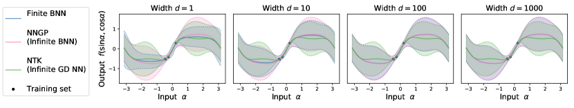
Figure 1: Posterior sample mean and variance of a deep finite BNN converge to those of an NNGP (infinite BNN) as width $d$ increases (left to right). For a given training set, posterior mean and variances are computed using rejection sampling for the finite BNN, and in closed form as a GP posterior (see (Rasmussen & Williams, 2006, page 16) for the NNGP, and Equation 16 in (Lee et al., 2019) for the NTK). As width $d$ increases, posterior predictions of a finite BNN and NNGP become indistinguishable, but clearly different from the NTK. Presented is a fully connected network with $L=3$ hidden layers and $\phi=$ Erf nonlinearities. All models use a Gaussian likelihood (Equation 2) with observation noise $\sigma^{2}=0.01$. NNGP and NTK predictions are computed with the Neural Tangents library (Novak et al., 2020). For each width $d\in\{1,10,100,1000\}$, a total of $2\cdot 10^{6}$ proposals are sampled, resulting in $3187$, $6796$, $8348$, and $8596$ accepts respectively. See Figure 2 for a numerical measure of convergence.

To understand Proposition 2, we can note that the ‘infinite-width, finite fan-out’ construction ensures the posterior marginal over ‘active’ parameters (those used in computation of the outputs) is exactly the posterior distribution we would have obtained had no extra parameters been introduced. Since convergence on the infinite dimensional space typically implies convergence of all finite-dimensional marginals, we can draw conclusions about the behaviour of the ‘active’ marginals.

However, the types of conclusions we can draw also show the crucial limitation of this approach. For example, $P_{\theta_{n}\operatorname{|}D}\Rightarrow P_{\theta}$ in the ‘infinite-width, finite fan-out’ sense implies that for any continuous bounded real-valued function $h$, $\operatorname*{\mathbb{E}}h(\theta_{n})\to\operatorname*{\mathbb{E}}h(\theta)$, including $h$ which only depend on the ‘active’ parameters of the $(n^{\prime})$^th network for any chosen $n^{\prime}$; unfortunately, this does not guarantee the expectations are close for the $(n^{\prime})$^th network itself! In other words, Proposition 2 tells us little about behaviour of finite BNNs.

One might still wonder about the $\delta_{0}$ limit under the standard parametrisation, since most NN architectures output a constant if all the parameters but biases are zero. This is due to the requirement that $P_{\theta_{n}}$ is selected such that $P_{f_{n}}$ converges, which will generally force each weight’s variance to vanish as $n\to\infty$ (see Equation 1 for an example). This typically translates into the same scaling under the posterior essentially because neurons in each layer are exchangeable (Matthews et al., 2018; Garriga-Alonso et al., 2019; Hron et al., 2020), implying no single parameter will be ‘pushed too far away’ from the prior by the likelihood (a similar effect can be seen in Example 1 in Appendix A). Since concentration in an increasingly ‘small’ region around zero is sufficient for weak convergence, the result follows.

Furthermore, we emphasise $P_{\theta}$ only describes a point in the distribution space to which the ‘infinite-width, finite fan-out’ $P_{\theta_{n}}$ converge, but should not be interpreted as a distribution over parameters of an infinitely wide BNN since the $\theta\mapsto f$ map for ‘$n=\infty$’ is not well-defined (as mentioned in Section 3). To see why, let us consider the single-layer FCN example with prior as in Equation 1. Our first impulse may be to define the $\gamma\colon\theta\mapsto f$ map as the pointwise limit of the functions $\gamma_{n}\colon\theta\mapsto f$ where each takes in a point $\theta\in\mathbb{R}^{\mathbb{N}}$ and computes the function implemented by the NN with corresponding index $n$ (as in Equation 5).

If the function $\gamma(\theta)$ is to be real-valued, we need

$$\gamma(\theta)(x)=\lim_{n\to\infty}\gamma_{n}(\theta)(x)=b^{2}+\lim_{n\to\infty}\sum_{i=1}^{0pt_{n}^{1}}w_{i}^{2}\phi(f_{i}^{1}(x))$$

to be well-defined and finite which is only true if $[w_{i}^{2}\phi(f_{i}^{1}(x))]_{i\in\mathbb{N}}$ is summable for each $x$ at the same time. This is not an issue under the standard parametrisation (since $w^{2}=0$ a.s.), but it is not satisfied under the NTK parametrisation where the support of $P_{\theta}$ is all of $\mathbb{R}^{\mathbb{N}}$.

Since the pointwise limit approach yields $f=b^{2}$ a.s. when $w^{2}=0$ a.s., and $f=\pm\infty$ a.s. or is undefined (if $\lim_{n\to\infty}\gamma_{n}(\theta)(x)$ does not exist) when $P_{\tilde{\theta}}$ has full $\mathbb{R}^{\mathbb{N}}$ support (NTK parametrisation), we may instead try to look for $\gamma$ satisfying $\gamma(\theta)\sim P_{f\operatorname{|}D}$, $\theta\sim P_{\theta\operatorname{|}D}$, for all possible finite $D$, with $P_{f\operatorname{|}D}$ the limit posterior from Proposition 1. As demonstrated, this is not satisfied by the pointwise limit. It also cannot be satisfied by any other deterministic $\gamma$ if $P_{\tilde{\theta}\operatorname{|}D}=\delta_{0}$, and there will be more than one solution if $P_{\theta\operatorname{|}D}$ has full support on $\mathbb{R}^{\mathbb{N}}$ (at least if we only require agreement on a fixed countable marginal of $P_{f\operatorname{|}D}$).

All in all, we see no obvious way of defining $\gamma$ without placing restrictive assumptions on $P_{\theta\operatorname{|}D}$. This is related to the dimensionality issue discussed at the beginning which forced us to adopt the additional ‘infinite-width, finite fan-out’ assumption. Since the ‘infinite-width, finite fan-out’ interpretation proved much less innocuous than in the case of input-to-output mappings where it is little more than a technicality (Matthews et al., 2018; Garriga-Alonso et al., 2019; Hron et al., 2020), we study two alternative choices in Appendix A. Unfortunately, neither yields a parameter space limit free of the pathologies we observed here.

5 Experimental validation

We sample from the exact finite BNN posterior using rejection sampling. For a given width $d_{n}$, we use $p_{\theta_{n}}$ as the proposal that envelops the unnormalised posterior density:

$$p(\theta\operatorname{|}\mathcal{Y},\mathcal{X}) \propto\ell(f_{\theta}(\mathcal{X}))p_{\theta_{n}}(\theta)\leq p_{\theta_{n}}(\theta),$$ (6)

where $\ell(f_{\theta}(\mathcal{X}))$ is the unnormalised Gaussian likelihood from Equation 2. Relatedly, prior sampling was recently used by Aitchison (2020) to estimate model evidence. Figures 1 and 2 confirm that as the finite BNN gets wider, its posterior mean and covariance converge to the NNGP ones.

6 Conclusion

We proved the sequence of exact posteriors of increasingly wide BNNs converges to the posterior induced by the infinite width limit of the prior and the same likelihood (when treated as a function of the NN outputs only). If the computation of the infinite width limit posterior is tractable, our result opens a path to tractable function space inference even if evaluation of parameter space posterior is intractable. We further studied conditions under which infinite width analysis in parameter space is possible and outlined several potential pitfalls. In experiments, we have shown how to draw samples from the exact BNN posterior on small datasets, and validated our function space convergence predictions. We hope our work provides theoretical basis for further study of exact BNN posteriors, and inspires development of more accurate BNN approximation techniques.

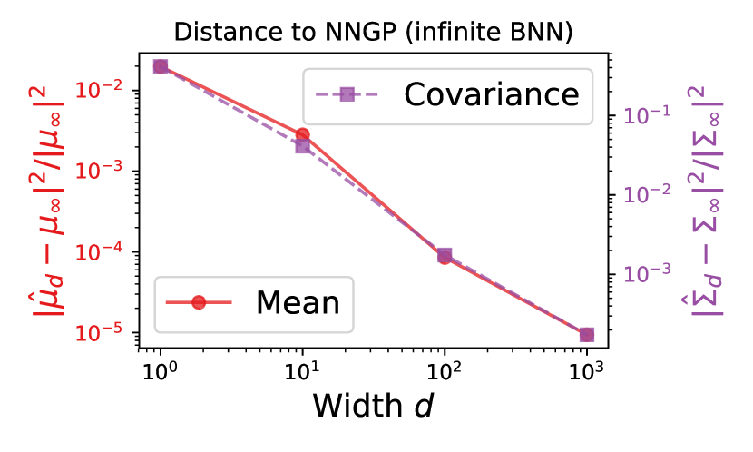
Figure 2: Posterior sample mean and covariance of a deep finite BNN converge to those of an NNGP (infinite BNN) as width $d$ increases (left to right, as measured by the relative Frobenius distance). Values evaluated at $100$ equidistant test points on $\left[-\pi;\pi\right]$. See Figure 1 for a visual demonstration and further details about the setup.

Appendix A Alternatives to the ‘infinite width, finite fan-out’ interpretation

The following is an (admittedly unconventional) attempt to gain intuition for the behaviour of parameter space posterior in wide BNNs by studying the simpler Bayesian linear regression model, and in particular, by measuring the discrepancy between the prior and the posterior of this model in 2-Wasserstein distance and Kullback-Leibler (KL) divergence.

Example 1.

Let $X\in\mathbb{R}^{m\times n}$ be a matrix of $m$ inputs and $y\in\mathbb{R}^{m}$ the vector of corresponding regression targets. Assume the usual Bayesian linear regression model $y\operatorname{|}X,w\sim\mathcal{N}(Xw,\beta I_{m})$, $w\sim\mathcal{N}(0,\frac{\alpha}{n}I_{n})$; to avoid notational clutter, we take $\alpha=\beta=1$. The induced posterior has closed form $w\sim\mathcal{N}(\mu_{n},\Sigma_{n})$ with

$$\Sigma_{n} =\left(nI_{n}+X^{\top}X\right)^{-1}$$

$$=\tfrac{1}{n}\left(I_{n}-\tfrac{1}{n}X^{\top}\left(I_{m}+\tfrac{1}{n}XX^{\top}\right)^{-1}X\right)\,,$$

$$\mu_{n} =\tfrac{1}{n}X^{\top}\left(I_{m}+\tfrac{1}{n}XX^{\top}\right)^{-1}y\,.$$

Note that if $X$ was replaced, e.g., by the outputs of FCN’s layer, $K_{n}\coloneqq\frac{1}{n}XX^{\top}$ would be converging almost surely to a constant $m\times m$ matrix as $n\to\infty$ (for an overview see, e.g., Yang, 2019a, b). To simplify our analysis, we assume the entries of $K_{n}$ are uniformly bounded with the implicit understanding that the results would have to be converted to high probability statements in order to hold for an actual BNN (e.g., using the results of Yang).

(I) We look at the squared 2-Wasserstein distance between the posterior and the prior

$$\mathcal{W}_{2}^{2}\left(\mathcal{N}(\mu_{n},\,\Sigma_{n}),\mathcal{N}(0,\tfrac{1}{n}I_{n})\right) =\|\mu_{n}\|_{2}^{2}+\mathrm{Tr}\left(\tfrac{1}{n}I_{n}+\Sigma_{n}-\tfrac{2}{\sqrt{n}}\Sigma_{n}^{1/2}\right)\,.$$

By the uniform entry bound assumption, $\|\mu_{n}\|_{2}\leq\frac{1}{n}[\lambda_{\text{min}}(I_{m}+K_{n})]^{-1}\|X\|_{2}\|y\|_{2}=\mathcal{O}(n^{-1/2})$ since $\|y\|_{2}$ is constant and $\frac{1}{\sqrt{n}}\|X\|_{2}=[\lambda_{\text{max}}(K_{n})]^{1/2}$, where $\lambda_{\text{min}}$ and $\lambda_{\text{max}}$ are the minimum and maximum eigenvalues. With a bit of algebra, one can also show that the value of the trace can be upper bounded by $\frac{m}{n}(1-(1+\lambda_{\text{min}}(K_{n}))^{-1/2})^{2}=\mathcal{O}(n^{-1})$. Hence the Wasserstein distance between the prior and the posterior shrinks to zero at $n^{-1/2}$ rate.

If we used the ‘infinite-width, finite fan-out’ construction, $\mathcal{N}(0,\frac{1}{n}I_{\mathbb{N}})$ would be converging weakly to $\delta_{0}$, and the same can be shown for the induced posterior analogously to Proposition 2. On one hand, the convergence of the prior-to-posterior 2-Wasserstein distance to zero could be interpreted as a confirmation of this result. On the other hand, $\mathcal{W}_{2}(\delta_{0},\mathcal{N}(0,\frac{1}{n}I_{n}))=1$ for all $n$, meaning that the prior (and thus the posterior) never approaches $\delta_{0}$ in $\mathcal{W}_{2}$. This is because $\mathcal{W}_{2}$ is defined w.r.t. the $\ell^{2}$ metric here which is inappropriate for $w\sim\mathcal{N}(0,\frac{1}{n}I_{\mathbb{N}})$ since such $w$ is not a.s. square summable.

(II) The KL-divergence between the posterior and the prior is

$$2\mathrm{KL}\left(\mathcal{N}(\mu_{n},\Sigma_{n})\,\|\,\mathcal{N}(0,\tfrac{1}{n}I_{n})\right) =n\|\mu_{n}\|_{2}^{2}-n+n\mathrm{Tr}(\Sigma_{n})-n\log n-\log|\Sigma_{n}|\,,$$

where we know that the sum of all the terms from the second to the last must be non-negative (it is equal to $2\mathrm{KL}(\mathcal{N}(0,\Sigma_{n})\,\|\,\mathcal{N}(0,\tfrac{1}{n}I_{n}))$). Hence we can lower bound by $n\|\mu_{n}\|_{2}^{2}$ which is order one (can be obtained analogously to the upper bound derived in our discussion of $\mathcal{W}_{2}$). This is perhaps not surprising as KL-divergence is lower bounded by (two times the square of) the total variation distance (Pinsker’s inequality) in which even $\mathcal{N}(0,\frac{1}{n}I_{k})$—for some fixed $k\in\mathbb{N}$—does not converge to $\delta_{0}$.

While Example 1 assumes the standard parametrisation, comparing to the conclusions that would have been drawn under the NTK parametrisation is instructive. Since the posterior remains Gaussian (with $\mu_{n}$ and $\Sigma_{n}$ scaled respectively by $\sqrt{n}$ and $n$), it is easy to check that KL-divergence remains unchanged (as it is invariant under any injective transformation), but the 2-Wasserstein distance grows by a multiplicative factor of $\sqrt{n}$ since

$$\mathcal{W}_{2}^{2}(\mathcal{N}(\sqrt{n}\mu_{n},n\Sigma_{n}),\mathcal{N}(0,I_{n})) =\inf_{\Gamma}\operatorname*{\mathbb{E}}_{(w_{0},w)\sim\Gamma}\|w_{0}-w\|_{2}^{2}$$

$$=n\,\inf_{\Gamma}\operatorname*{\mathbb{E}}_{(w_{0},w)\sim\Gamma}\biggl{\|}\frac{w_{0}}{\sqrt{n}}-\frac{w}{\sqrt{n}}\biggr{\|}_{2}^{2}=n\,\mathcal{W}_{2}^{2}(\mathcal{N}(\mu_{n},\Sigma_{n}),\mathcal{N}(0,I_{n}))\,,$$

where the infinum ranges over all joint distributions $\Gamma$ on $\mathbb{R}^{2n}$ which have $\mathcal{N}(\sqrt{n}\mu_{n},n\Sigma_{n})$ and $\mathcal{N}(0,I_{n})$ as their respective $n$-dimensional marginals. In other words, the prior-to-posterior Wasserstein distance does not converge to zero when Euclidean distance is used (it will converge to zero when used with the metric from Footnote 8 though, which is why the above is not a contradiction of Proposition 2; cf. the last statement in (I), Example 1).

The above implies we need to be careful in interpreting rates of convergence, and in particular, that some discrepancy measures like the Wasserstein metrics necessitate choice of measurement unit for the parameters. KL-divergence does not suffer from such issues but its relation with the total variation distance could make it excessively strict (total variation distance implies weak convergence but the reverse is not true; see the example in the last statement in (II) in Example 1).

While we cannot offer a definite answer to the above issues, it is worth pointing out that what we care about in practice is the accuracy of the function space approximation where issues of changing dimensionality disappear, and measurement units are dictated by the dataset we are trying to model. Hence a potentially more fruitful approach would be to refocus our attention from the parameter space to measurement and optimisation of function space approximation accuracy.

Appendix B Proofs

Proof of Proposition 1.

By the definition of weak convergence, all we need to show is that for any continuous bounded function $h\colon f\mapsto h(f)\in\mathbb{R}$, the expectation converges $\int\!h\,\mathrm{d}P_{f_{n}\operatorname{|}D}\to\int\!h\,\mathrm{d}P_{f\operatorname{|}D}$. The key observation is that 1 ensures each posterior $P_{f_{n}\operatorname{|}D}$ has a density w.r.t. the prior (e.g. Schervish, 2012, theorem 1.31)

$$\frac{\mathrm{d}P_{f_{n}\operatorname{|}D}}{\mathrm{d}P_{f_{n}}}(f)=\frac{\ell(f(\mathcal{X}))}{Z_{n}}\,,$$

where $Z_{n}\coloneqq\int\!\ell\,\mathrm{d}P_{f_{n}}$. Substituting

$$\int\!h(f)\,\mathrm{d}P_{f_{n}\operatorname{|}D}(f)=\frac{1}{Z_{n}}\int\!h(f)\ell(f(\mathcal{X}))\,\mathrm{d}P_{f_{n}}(f)\,.$$

Since $\ell$ is continuous bounded and $Z=\int\!\ell\,\mathrm{d}P_{f}>0$ by assumption, $Z_{n}\to Z$ by $P_{f_{n}}\Rightarrow P_{f}$. Similarly, $f\mapsto h(f)\ell(f(\mathcal{X}))$ is continuous bounded, and thus also

$$\int\!h(f)\ell(f(\mathcal{X}))\,\mathrm{d}P_{f_{n}}(f)\to\int\!h(f)\ell(f(\mathcal{X}))\,\mathrm{d}P_{f}(f)\,.$$

The proof is concluded by observing theorem 1.31 (Schervish, 2012) applies also to the density of $P_{f\operatorname{|}D}$ w.r.t. $P_{f}$. ∎

Proof of Corollary 1.

Following the proof strategy of Proposition 1

$$\int\!h\,\mathrm{d}P_{f_{n}\operatorname{|}D}=\frac{1}{Z_{n}}\int\!h({f})\ell({f}(\mathcal{X}))\,\mathrm{d}P_{f_{n}}({f})\,,$$

we see that all we need to prove is the convergence of the integral on the right hand side ($Z_{n}\to Z$ established in Proposition 1). Let $f_{n}\sim P_{f_{n}}$ and $f\sim P_{f}$. Since $h$ is continuous, $|h(f_{n})|\Rightarrow|h(f)|$ by the continuous mapping theorem. Because the expectation of $|h|$ converges under the prior by assumption, $\{h(f_{n})\}_{n\geq 1}$ is uniformly integrable by theorem 3.6 in (Billingsley, 1986). Because $\ell$ is bounded by assumption, $\{h(f_{n})\ell(f_{n}(\mathcal{X}))\}_{n\geq 1}$ is uniformly integrable as well by definition. Since $h(f_{n})\ell(f_{n}(\mathcal{X}))\Rightarrow h(f)\ell(f(\mathcal{X}))$ by the continuous mapping theorem again

$$\int\!h({f})\ell({f}(\mathcal{X}))\,\mathrm{d}P_{f_{n}}({f})\to\int\!h({f})\ell({f}(\mathcal{X}))\,\mathrm{d}P_{f}({f})\,,$$

by theorem 3.5 in (Billingsley, 1986). ∎

Proof of Proposition 2.

By (Billingsley, 1986, theorem 2.4), it will be sufficient to prove convergence of finite dimensional marginals of $P_{\theta_{n}\operatorname{|}D}$. Denoting indices of this marginal by $J$ and the corresponding sequence of marginal distributions by $P_{\theta_{n}^{J}\operatorname{|}D}$, all we need to establish is that for any continuous bounded real-valued function $h$, $\int\!h\,\mathrm{d}P_{\theta_{n}^{J}\operatorname{|}D}\to\int\!h\,\mathrm{d}P_{\theta^{J}}\,.$ By 1, we can rewrite both the integrals in terms of the prior; for the $\int\!h\,\mathrm{d}P_{\theta_{n}^{J}\operatorname{|}D}$ this yields

$$\int\!h\,\mathrm{d}P_{\theta_{n}^{J}\operatorname{|}D}=\frac{1}{Z_{n}}\int\!h(\theta^{J})\ell(f_{\theta}(\mathcal{X}))\,\mathrm{d}P_{\theta_{n}}(\theta)\,,$$

where $\theta^{J}$ denotes the appropriate subset of entries of $\theta$, and $Z_{n}=\int\!\ell(f_{\theta}(\mathcal{X}))\,\mathrm{d}P_{\theta_{n}}(\theta)$. By the same argument as in the proof of Proposition 1, $Z_{n}\to Z=\int\ell(f(\mathcal{X}))\,\mathrm{d}P_{f}(f)$ where $Z>0$ by assumption. Hence we can focus on

$$\int\!h(\theta^{J})\ell(f_{\theta}(\mathcal{X}))\,\mathrm{d}P_{\theta_{n}}(\theta)=\int\!h(\theta^{J})\int\!\ell(f_{\theta}(\mathcal{X}))\mathrm{d}P_{\theta_{n}^{\mathbb{N}\setminus J}}(\theta^{\mathbb{N}\setminus J})\,\mathrm{d}P_{\theta_{n}^{J}}(\theta^{J})$$

where $\theta^{\mathbb{N}\setminus J}$ are all the entries of $\theta$ not in $J$, and the equality is by boundedness of both $h$ and $\ell$, the Tonelli-Fubini theorem, and diagonal Gaussian prior (implying $P_{\theta_{n}^{\mathbb{N}\setminus J}\operatorname{|}\theta_{n}^{J}}=P_{\theta_{n}^{\mathbb{N}\setminus J}}$ for all $\theta^{J}$). Also by the diagonal Gaussian assumption, we can use the change of variable formula to replace any weight $\theta_{i}$ by $\theta_{i}(\varepsilon)=\sigma\varepsilon_{i}/\sqrt{0pt_{n}^{l}}$ for an appropriate $l$ and $\varepsilon_{i}\sim\mathcal{N}(0,1)$ i.i.d. (this step is of course not necessary under the NTK parametrisation). The r.h.s. above can then be rewritten as

$$\int\!h_{n}(\varepsilon^{J})z_{n}(\varepsilon^{J})\mathrm{d}P_{\varepsilon^{J}}(\varepsilon^{J})\,,$$

where

$$h_{n}(\varepsilon^{J})\coloneqq h(\theta^{J}(\varepsilon^{J}))\,,\qquad z_{n}(\varepsilon^{J})\coloneqq\int\!\ell(f_{\theta^{J}(\varepsilon^{J})\cup\theta^{\mathbb{N}\setminus J}}(\mathcal{X}))\mathrm{d}P_{\theta_{n}^{\mathbb{N}\setminus J}}(\theta^{\mathbb{N}\setminus J})\,.$$

Let us assume there are no top-layer biases for now, and add them back at a later point. Our current goal is to show that $h_{n}(\varepsilon^{J})z_{n}(\varepsilon^{J})\to h_{\star}(\varepsilon^{J})Z$ pointwise for some function $h_{\star}\colon\mathbb{R}^{J}\to\mathbb{R}$ such that $\int\!h_{*}(\varepsilon^{J})\,\mathrm{d}P_{\varepsilon^{J}}(\varepsilon^{J})=\int\!h(\theta^{J})\,\mathrm{d}P_{\theta}^{J}(\theta^{J})$ for $P_{\theta^{J}}=\delta_{0^{J}}$ under the standard, and $P_{\theta^{J}}=\mathcal{N}(0,I_{|J|})$ under the NTK parametrisation. Since both $h$ and $\ell$ are bounded by assumption, $h_{n}\cdot z_{n}$ are uniformly bounded and thus the pointwise convergence could be combined with the dominated convergence theorem to conclude the proof. Since $h$ is continuous by assumption, $h_{*}(\varepsilon^{J})=h(0)$ under the standard, and $h_{*}(\varepsilon^{J})=h(\varepsilon^{J})$ for all $\varepsilon^{J}$ values under the NTK parametrisation. One can easily verify that $\int\!h_{*}(\varepsilon^{J})\,\mathrm{d}P_{\varepsilon^{J}}(\varepsilon^{J})=\int\!h(\theta^{J})\,\mathrm{d}P_{\theta}^{J}(\theta^{J})$ in both cases as required. All that remains is thus to show $z_{n}\to Z$ pointwise.

To do so, we will show that fixing a finite set of parameters while letting the others vary does not affect the convergence of the induced input-to-output mappings $P_{f_{n}\operatorname{|}\varepsilon^{J}}\Rightarrow P_{f}$ where $P_{f_{n}\operatorname{|}\varepsilon^{J}}$ denotes the function space distribution given the fixed $\varepsilon^{J}$. We achieve this by a modification of the proof techniques in (Matthews et al., 2018; Garriga-Alonso et al., 2019; Hron et al., 2020). The arguments therein are invariably build around an inductive application of the central limit theorem for infinitely exchangeable triangular arrays (eCLT) due to Blum et al. (1958) to linear projections of a finite subset of units. Since convergence in distribution of all such projections implies pointwise convergence of the characteristic function ($x\mapsto e^{\sqrt{-1}x}$ is continuous bounded), convergence in distribution follows. It will thus be sufficient to show how to modify the recursive application of the eCLT.

What follows is a high-level description of this modification; a detailed description showcasing how to fill in the details on the FCN example can be found in Section B.1. Let us consider layer $l\geq 2$ and the corresponding vector of activations $f_{n}^{l}(\mathcal{X})=\{f_{n,i}^{l}(x)\}_{(x,i)\in\mathcal{X}\times\mathbb{N}}$ (by the definition of $z_{n}$, we only need weak convergence of $f_{n}$ evaluated on the training set). By theorem 2.4 in (Billingsley, 1986), weak convergence is implied by weak convergence of all finite marginals. Denote the indices of these final marginals by $K$, and define $f_{n}^{l,K}(\mathcal{X})=\{f_{n,i}^{l}(x)\}_{(x,i)\in\mathcal{X}\times K}$.

As mentioned, weak convergence of $f_{n}^{l,K}(\mathcal{X})$ is implied by weak convergence of linear projections, so fix a vector $\alpha\in\mathbb{R}^{K}$, and consider the scalar random variable $\langle\alpha,f_{n}^{l,K}(\mathcal{X})\rangle$. Conveniently, $\langle\alpha,f_{n}^{l,K}(\mathcal{X})\rangle$ can always be rewritten as

$$\frac{1}{\sqrt{0pt_{n}^{l-1}}}\sum_{j\in B_{n}}c_{n,j}\varepsilon_{j}^{l}\,,$$

for some (random) coefficients $c_{n,j}$, and a subset of indices $B_{n}\subset\mathbb{N}$ s.t. $|B_{n}|=0pt_{n}^{l-1}$, $B_{n}\subseteq B_{n+1}$ for all $n\in\mathbb{N}$. Here $c_{n,j}$ are essentially a combination of the projection coefficients $\alpha$ and the inputs to the layer, whereas $\varepsilon_{j}^{l}$ are the Gaussian random variables constituting $\theta^{l}(\varepsilon^{l})$ (either directly under NTK, or by reparametrisation under standard parametrisation); see Equations 8, 9 and 10 for an example.

Defining $B\coloneqq\bigcup_{n}B_{n}$, for all $n$ large enough

$$\frac{1}{\sqrt{0pt_{n}^{l-1}}}\sum_{j\in B_{n}}c_{n,j}\varepsilon_{j}^{l}=\frac{1}{\sqrt{0pt_{n}^{l-1}}}\sum_{i\in J\cap B}c_{n,i}\varepsilon_{i}^{l}+\frac{\sqrt{0pt_{n}^{l-1}-|J|}}{\sqrt{0pt_{n}^{l-1}}}\frac{1}{\sqrt{0pt_{n}^{l-1}-|J|}}\sum_{j\in B_{n}\setminus J}c_{n}^{j}\varepsilon^{j}\,.$$ (7)

Using $|J|<\infty$, the first term on the r.h.s. can be shown to converge to zero in probability. Since $[0pt_{n}^{l-1}-|J|)/0pt_{n}^{l-1}]^{1/2}\to 1$, and the remaining sum is properly scaled by $(0pt_{n}^{l-1}-|J|)^{1/2}$, an argument analogous to that of Matthews et al. can be used to establish it converges in distribution to the desired limit as it does not depend on any of the fixed parameters in the $l$^th layer, and dependence on the fixed values in the previous layers vanishes as $n\to\infty$ by the recursive application of the above argument (of course there are no terms that depend on the fixed values for $j\in B_{n}\setminus J$ when $l=2$). A simple application of Slutsky’s lemmas (if $X_{n}\Rightarrow X$ and $Y_{n}\to c$ in probability, $c\in\mathbb{R}$, then $X_{n}+Y_{n}\Rightarrow X+c$, and $X_{n}Y_{n}\Rightarrow cX$) then yields that for any fixed values of $\langle\alpha,f_{n}^{l,K}(\mathcal{X})\rangle$ converges in distribution to the desired limit. Hence, $P_{f_{n}\operatorname{|}\varepsilon^{J}}\Rightarrow P_{f}$ for any fixed value of $\varepsilon^{J}$ as desired.

All that remains is to add back the top-layer biases. As we have seen, the $P_{f_{n}\operatorname{|}\varepsilon^{J}}$ distribution without top-layer biases converges to $P_{f-b^{0pt+1}}$ (the prior limit after subtraction of top-layer biases), and thus the biases may be simply added on top. In the case of a Gaussian $P_{f}$, this will result in an additive $\sigma_{b}^{2}$ term in the covariance matrix as usual (this can be proved by standard argument via characteristic function using the assumed Gaussian diagonal prior over all parameters). The posterior over the top-layer biases will then be same as if we did joint posterior update over $f\sim P_{f-b^{0pt+1}}$ and $b^{0pt+1}$ a prior distributed according to the weak limit of the corresponding marginals of $P_{\theta_{n}}$. ∎

B.1 Proving $z_{n}(\varepsilon^{J})\to Z$ pointwise in a fully-connected network

Note: All of the references to (Matthews et al., 2018) here are to the version accessible at https://arxiv.org/abs/1804.11271v2

The goal of this section is to adapt the original proof by Matthews et al. (2018). We thus omit introduction of the notation as well as substantial discussion of the steps that do not require modifications. We also modify our notation to match that of Matthews et al. to make comparison easier. It is thus advisable to consult section 2 in (Matthews et al., 2018) which introduces the general notation before reading on, and then referring to section 6 whenever necessary.

We can follow the same steps as Matthews et al. right until the application of the Cramér-Wold device and definition of projections $\mathcal{T}$ and summands $\gamma$ (Matthews et al., 2018, p. 19-20). The application of eCLT (resp. its modified version (Matthews et al., 2018, p. 22, lemma 10)) essentially reduces the problem of establishment of weak convergence of $f_{n}$ to that of proving of convergence of its first few finite-dimensional moments. Following Matthews et al., we define the projections $\mathcal{T}$ and summands $\gamma$ as in their equations (25) to (27) which we restate here for convenience:

$$\mathcal{T}^{(l)}[n] \coloneqq\sum_{(x,i)\in\mathcal{L}}\alpha^{(x,i)}\left[{f}^{l}_{i}{(x)}[n]-{b}^{l}_{i}{}\right]\,,$$ (8)

$$\gamma^{(l)}_{j}[n] \coloneqq\sum_{(x,i)\in\mathcal{L}}\alpha^{(x,i)}{\varepsilon}^{l}_{i,j}{}{g}^{l-1}_{j}{(x)}[n]\sqrt{\hat{C}_{w}^{(l)}}\,,$$ (9)

$$\mathcal{T}^{(l)}[n] =\frac{1}{\sqrt{h^{l-1}(n)}}\sum_{j=1}^{h^{l-1}(n)}\gamma^{(l)}_{j}[n]\,.$$ (10)

Here ${g}^{l}_{i}{(x)}[n]=\phi({f}^{l}_{i}{(x)}[n])$ is the $i$^th post-nonlinearity in $l$^th layer of the $n$^th network evaluated at point $x$, $h^{l}(n)$ is the width of the same layer, $\mathcal{L}\subset\mathcal{X}\times\mathbb{N}$ identifies the finite marginal of the countably infinite vector $\{{f}^{l}_{i}{(x)}\}_{(x,i)\in\mathcal{X}\times\mathbb{N}}$ under consideration, and $\alpha=\{\alpha^{(x,i)}\}_{(x,i)\in\mathcal{L}}\in\mathbb{R}^{\alpha}$ is the Cramér-Wold projection vector.

Note that Matthews et al. define ${f}^{l}_{i}{(x)}[n]$ as the sum of the inner product of the relevant weight vector with ${g}^{l-1}_{i}{(x)}[n]$ and the bias term ${b}^{l}_{i}{}$, which is why ${b}^{l}_{i}{}$ is subtracted in Equation 8. In contrast, we omitted subtraction of ${b}^{l}_{i}{}$ in the previous section to reduce the notational clutter. From now on, we stick with the notation of Equations 8, 9 and 10. Last point where our notation differs from Matthews et al. is in omitting the dependence of $\mathcal{T}^{(l)}[n]$ and $\gamma^{(l)}_{j}[n]$ on $\mathcal{L}$ and $\alpha$ (the original notation was $\mathcal{T}^{(l)}(\mathcal{L},\alpha)[n]$ and $\gamma^{(l)}_{j}(\mathcal{L},\alpha)[n]$).

Our goal is to prove convergence of the outputs $\{{f}^{0pt+1}_{i}{(x)}\}_{(x,i)\in\mathcal{X}\times\mathbb{N}}$ given that a finite subset of $\{{\varepsilon}^{l}_{i,j}{}\}_{\begin{subarray}{c}i,j\in\mathbb{N}\\ \end{subarray};1\leq l\leq 0pt+1}$ is fixed to an arbitrary value. As in (Matthews et al., 2018), we approach this problem by an inductive application of their lemma 10 to the projections $\mathcal{T}$ combined with theorem 3.5 from (Billingsley, 1986). We will thus need to prove the sums defined in Equation 10 satisfy all the desired properties for any choice of $\mathcal{L}$, $\alpha\in\mathbb{R}^{\mathcal{L}}$, and $l=2,\ldots,0pt+1$; recall that $f^{1}$ corresponds to the pre-nonlinearities in the first layer and thus even for a single layer neural network, $f^{2}$ is the output. This is important because the input dimension is fixed and thus the distribution of $f^{1}$ need not be Gaussian for a given $\varepsilon^{J}$ as we can trivially select $|J|$ bigger than the input dimension and thus control value of any finite subset of the pre-nonlinearities in the first layer. As you may suspect, the fact that we can only ever affect a finite subset of these activations will be crucial in the next paragraphs.

We turn to applying lemma 10 from (Matthews et al., 2018) for $l\geq 2$. As the lemma applies only to exchangeable sequences, our first step will be to isolate the non-exchangeable terms. Matthews et al. prove exchangeability of the summands $\gamma_{j}^{(l)}[n]$ over the index $j$ in their lemma 8. The key observation here is that the same proof still works if we exclude all indices $j$ s.t. $\exists\,i\in\mathcal{L}_{\mathbb{N}}$ with ${\varepsilon}^{l}_{i,j}{}\in\varepsilon^{J}$ (where $\mathcal{L}_{\mathbb{N}}$ is the set of width indices in $\mathcal{L}$), i.e., if we exclude all summands for which at least one weight is fixed through $\varepsilon^{J}$. Defining $J^{l}\coloneqq\{j\in\mathbb{N}\colon\exists\,i\in\mathcal{L}_{\mathbb{N}}\text{ s.t.\ }{\varepsilon}^{l}_{i,j}{}\in\varepsilon^{J}\}$, we can rewrite Equation 10 as

$$\mathcal{T}^{(l)}[n]=\frac{\sum_{i\in J^{l}}\gamma^{(l)}_{i}[n]}{\sqrt{h^{l-1}(n)}}+\frac{\sqrt{h^{l-1}(n)-|J^{l}|}}{\sqrt{h^{l-1}(n)}}\frac{\sum_{j\in[h^{l-1}(n)]\setminus J^{l}}\gamma^{(l)}_{j}[n]}{\sqrt{h^{l-1}(n)-|J^{l}|}}\,,$$ (11)

which mirrors the format of Equation 7 from the previous section.

Our next step is thus to apply Slutsky’s lemmas, which in particular means that we need to show that the first term on the r.h.s. of Equation 11 converges in probability to zero, and the second in distribution to the relevant GP limit as in (Matthews et al., 2018). We will start with the first term. Let us define

$$\gamma^{(l)}_{j}[n] \coloneqq\alpha^{\top}\tilde{g}_{j}^{l}[n] j\in\mathbb{N}\,,$$

$$\tilde{g}_{j}^{l}[n]_{i} \coloneqq{\varepsilon}^{l}_{(i),j}{}{g}^{l-1}_{j}{(x_{(i)})}[n] i\in\{1,\ldots,|\mathcal{L}|\}\,,$$

as in (Matthews et al., 2018, appendix B.1) and also, to reduce notational clutter, w.l.o.g. assume the weight variance scaling $\hat{C}_{w}^{(l)}$ is equal to one $\forall l$. Now observe

$$\biggl{|}\frac{1}{\sqrt{h^{l-1}(n)}}\sum_{i\in J^{l}}\gamma^{(l)}_{i}[n]\biggr{|}\leq\frac{1}{\sqrt{h^{l-1}(n)}}\sum_{i\in J^{l}}\|\alpha\|_{2}\|\tilde{g}_{i}^{l}[n]\|_{2}\qquad\text{a.s.}\,,$$ (12)

by a simple application of the Cauchy-Schwarz inequality. Since $|J^{l}|<\infty$ and $\|\alpha\|_{2}<\infty$, an easy approach of showing that the sum converges in probability to zero is to apply the Markov’s inequality to obtain that for any $\delta>0$

$$\operatorname{\mathbb{P}}\biggl{(}\sum_{i\in J^{l}}\|\tilde{g}_{i}^{l}[n]\|_{2}\geq\sqrt{h^{l-1}(n)}\delta\biggr{)}\leq\frac{\operatorname*{\mathbb{E}}\biggl{[}\biggl{(}\sum_{i\in J^{l}}\|\tilde{g}_{i}^{l}[n]\|_{2}\biggr{)}^{2}\biggr{]}}{\delta^{2}h^{l-1}(n)}\leq\frac{|J^{l}|\sum_{i\in J^{l}}\operatorname*{\mathbb{E}}\|\tilde{g}_{i}^{l}[n]\|_{2}^{2}}{\delta^{2}h^{l-1}(n)}\,,$$

where we have used $(\sum_{k=1}^{K}|x_{k}|)^{2}\leq K(\max(|x_{1}|,\ldots|x_{K}|))^{2}\leq K\sum_{k=1}^{K}x_{k}^{2}$. Hence a sufficient condition for convergence to zero in probability is that the expected norms of the activations over $\mathcal{L}$ converge to a constant. By definition

$$\operatorname*{\mathbb{E}}\|\tilde{g}_{j}^{l}[n]\|_{2}^{2}=\sum_{(x,i)\in\mathcal{L}}\operatorname*{\mathbb{E}}[({\varepsilon}^{l}_{i,j}{})^{2}]\operatorname*{\mathbb{E}}[({g}^{l-1}_{j}{(x)}[n])^{2}]\,.$$

Since $\operatorname*{\mathbb{E}}[({\varepsilon}^{l}_{i,j}{})^{2}]\leq\max(1,\max_{j\in J}(\varepsilon^{j})^{2})<\infty$, and by the ‘linear envelope condition’ $\operatorname*{\mathbb{E}}[({g}^{l-1}_{j}{(x)}[n])^{2}]\leq 2(c^{2}+m^{2}\operatorname*{\mathbb{E}}[({f}^{l-1}_{j}{(x)}[n])^{2}])$, we can establish the convergence by proving lemma 20 from (Matthews et al., 2018) still holds.

Since lemma 20 from (Matthews et al., 2018) is also necessary to prove that the second term on the r.h.s. of Equation 11 converges, we now turn to this latter term. As already mentioned, our strategy for the latter term will be to prove its convergence in distribution using lemma 10 from (Matthews et al., 2018). Aligning the notation by substituting $X_{n,j}=\gamma^{(l)}_{j}[n]$ so that

$$S_{n}=\frac{1}{\sqrt{h^{l-1}(n)-|J^{l}|}}\sum_{j\in[h^{l-1}(n)]\setminus J^{l}}\gamma^{(l)}_{j}[n]\,,$$ (13)

we satisfy exchangeability by definition of $J^{l}$, and $\operatorname*{\mathbb{E}}\gamma^{(l)}_{i}[n]=0$ as well as $\operatorname*{\mathbb{E}}\gamma^{(l)}_{j}[n]\gamma^{(l)}_{j}[n]=0$ hold as long as lemma 20 from (Matthews et al., 2018) is true so that $\operatorname*{\mathbb{E}}|{g}^{l-1}_{j}{(x)}[n]|^{2}<\infty$ (since $\operatorname*{\mathbb{E}}{\varepsilon}^{l}_{i,j}{}=0$ for all $j\in\mathbb{N}\setminus J^{(l)})$. Finiteness of variance and the absolute third moments as well as $\sigma_{\star}^{2}=\lim_{n}\sigma_{n}^{2}\coloneqq\lim_{n\to\infty}\operatorname*{\mathbb{V}}(\gamma^{(l)}_{j}[n])$ will be established in course of proving that the conditions b) $\lim_{n\to\infty}\operatorname*{\mathbb{E}}\gamma^{(l)}_{i}[n]^{2}\gamma^{(l)}_{j}[n]^{2}=\sigma_{\star}^{4}$, and c) $\operatorname*{\mathbb{E}}|\gamma^{(l)}_{j}[n]|^{3}=\mathrm{o}(\sqrt{h^{l-1}(n)-|J^{l}|})$ of lemma 10 from (Matthews et al., 2018) still hold.

We thus turn to proving conditions b) and c) are satisfied for any fixed value of $\varepsilon^{J}$. In the original paper, this is accomplished respectively in lemmas 15 and 16. On closer inspection, fixing $\varepsilon^{J}$ can only affect the proofs of these lemmas by invalidating lemma 20 or 21 from (Matthews et al., 2018). Lemma 20 establishes that for any fixed input $x\in\mathcal{X}$, $\operatorname*{\mathbb{E}}|{f}^{l}_{i}{(x)}|^{8}$ is bounded by a constant independent of $n$ and $i$, for all $l\in[0pt+1]$. As in the original proof, we proceed by induction. For $l=1$, the distribution of ${f}^{l}_{i}{(x)}$ is Gaussian or a Dirac’s delta distribution which is either zero mean (if $i\notin J^{(1)}$), or centred at some point in $\mathbb{R}$ determined by the ${\varepsilon}^{1}_{i,j}{}\in\varepsilon^{J}$. In either case, the eighth moments will be finite by basic properties of univariate Gaussian distributions. This bound will be independent of $n$ by definition of $f^{1}(x)$, and of $i$ by finiteness of $J^{1}$ and exchangeability of the remaining terms.

As in the original, we proceed by induction. Assume that the condition holds for all $l=1,2,\ldots,t-1$ (for some $t\in\{2,\ldots,0pt+1\}$). Then

$$\operatorname*{\mathbb{E}}|{f}^{t}_{i}{(x)}[n]|^{8}\leq 2^{8-1}\operatorname*{\mathbb{E}}\biggl{[}|b_{i}^{t}|^{8}+\biggl{|}\sum_{j=1}^{h^{t-1}(n)}w_{i,j}^{t}g_{j}^{t-1}(x)[n]\biggr{|}^{8}\biggr{]}\,.$$

Immediately, $\sup_{i}\operatorname*{\mathbb{E}}|b_{i}^{t}|^{8}<\infty$ by $|J|<\infty$ and Gaussianity of the other biases. Moving on to the second term, we can upper bound the expectation

$$\operatorname*{\mathbb{E}}\biggl{|}\sum_{j=1}^{h^{t-1}(n)}w_{i,j}^{t}g_{j}^{t-1}(x)[n]\biggr{|}^{8} \leq 2^{8-1}\operatorname*{\mathbb{E}}\biggl{|}\sum_{j\in J^{t}}w_{i,j}^{t}g_{j}^{t-1}(x)[n]\biggr{|}^{8}+\biggl{|}\sum_{j\in[h^{t-1}(n)]\setminus J^{t}}w_{i,j}^{t}g_{j}^{t-1}(x)[n]\biggr{|}^{8}\,,$$

The rest of the argument in lemma 20 (Matthews et al., 2018) still holds for the sum over $j\in[h^{t-1}(n)]\setminus J^{t}$ which will give us a constant bound on its contribution independent of $n$ and $i$. For the other term, we have

$$\operatorname*{\mathbb{E}}\biggl{|}\sum_{j\in J^{t}}w_{i,j}^{t}g_{j}^{t-1}(x)[n]\biggr{|}^{8}\leq\frac{2^{8-1}|J^{t}|}{|h^{t-1}(n)|^{4}}\sum_{j\in J^{t}}\operatorname*{\mathbb{E}}[|{\varepsilon}^{t}_{i,j}{}|^{8}](c^{8}+m^{8}\operatorname*{\mathbb{E}}|{f}^{t-1}_{i}{(x)}[n]|^{8})\,,$$

and thus we can again upper bound by a constant independent of $n$ and $i$ using $|J^{t}|<\infty$, $\operatorname*{\mathbb{E}}|{\varepsilon}^{t}_{i,j}{}|^{8}\leq\max(1,\max_{j\in J}|\varepsilon^{j}|^{8})$, $|h^{t-1}(n)|^{4}\geq 1$, and the inductive hypothesis on $\operatorname*{\mathbb{E}}|{f}^{t-1}_{i}{(x)}[n]|^{8}$. This concludes the proof of lemma 20.

The last outstanding task is thus to check that lemma 21 from (Matthews et al., 2018) holds for any fixed $\varepsilon^{J}$. Inspecting the original proof, the argument therein holds when we substitute the strengthened version of the lemma 20 from above. Recalling that the updated version of lemma 20 was also the only thing needed to finish the proof that the first term in Equation 13 converges in probability to zero, the above implies that $S_{n}$ from the same equation converges in probability to the desired limit. We can thus proceed with application of Slutsky’s lemmas as described in the previous section, concluding $z_{n}\to Z$ pointwise as desired.

References

• Aitchison (2020) Aitchison, L. Why bigger is not always better: on finite and infinite neural networks. In International Conference on Machine Learning, 2020.
• Billingsley (1986) Billingsley, P. Probability and Measure. John Wiley and Sons, second edition, 1986.
• Blum et al. (1958) Blum, J. R., Chernoff, H., Rosenblatt, M., and Teicher, H. Central limit theorems for interchangeable processes. Canadian Journal of Mathematics, 10:222–229, 1958.
• Garriga-Alonso et al. (2019) Garriga-Alonso, A., Rasmussen, C. E., and Aitchison, L. Deep convolutional networks as shallow Gaussian processes. In International Conference on Learning Representations, 2019.
• Hron et al. (2020) Hron, J., Bahri, Y., Sohl-Dickstein, J., and Novak, R. Infinite attention: NNGP and NTK for deep attention networks. In International Conference on Machine Learning, 2020.
• Jacot et al. (2018) Jacot, A., Gabriel, F., and Hongler, C. Neural tangent kernel: Convergence and generalization in neural networks. In Advances in Neural Information Processing Systems, 2018.
• Lee et al. (2018) Lee, J., Sohl-dickstein, J., Pennington, J., Novak, R., Schoenholz, S., and Bahri, Y. Deep neural networks as Gaussian processes. In International Conference on Learning Representations, 2018.
• Lee et al. (2019) Lee, J., Xiao, L., Schoenholz, S. S., Bahri, Y., Novak, R., Sohl-Dickstein, J., and Pennington, J. Wide neural networks of any depth evolve as linear models under gradient descent. In Advances in Neural Information Processing Systems, 2019.
• Matthews et al. (2018) Matthews, A. G., Rowland, M., Hron, J., Turner, R. E., and Ghahramani, Z. Gaussian process behaviour in wide deep neural networks. arXiv preprint arXiv:1804.11271, 2018.
• Neal (1996) Neal, R. M. Bayesian Learning for Neural Networks. Springer, 1996.
• Novak et al. (2019) Novak, R., Xiao, L., Bahri, Y., Lee, J., Yang, G., Hron, J., Abolafia, D. A., Pennington, J., and Sohl-Dickstein, J. Bayesian deep convolutional networks with many channels are Gaussian processes. In International Conference on Learning Representations, 2019.
• Novak et al. (2020) Novak, R., Xiao, L., Hron, J., Lee, J., Alemi, A. A., Sohl-Dickstein, J., and Schoenholz, S. S. Neural tangents: Fast and easy infinite neural networks in python. In International Conference on Learning Representations, 2020.
• Rasmussen & Williams (2006) Rasmussen, C. E. and Williams, C. K. Gaussian processes for machine learning, volume 1. MIT press Cambridge, 2006.
• Schervish (2012) Schervish, M. J. Theory of statistics. Springer Science & Business Media, 2012.
• Sohl-Dickstein et al. (2020) Sohl-Dickstein, J., Novak, R., Schoenholz, S. S., and Lee, J. On the infinite width limit of neural networks with a standard parameterization. arXiv preprint arXiv:2001.07301, 2020.
• Yang (2019a) Yang, G. Scaling limits of wide neural networks with weight sharing: Gaussian process behavior, gradient independence, and neural tangent kernel derivation. arXiv preprint arXiv:1902.04760, 2019a.
• Yang (2019b) Yang, G. Wide feedforward or recurrent neural networks of any architecture are Gaussian processes. In Advances in Neural Information Processing Systems 32, pp. 9947–9960. Curran Associates, Inc., 2019b.