SE(3)-Transformers: 3D Roto-Translation Equivariant Attention Networks

Abstract

We introduce the SE(3)-Transformer, a variant of the self-attention module for 3D point clouds and graphs, which is equivariant under continuous 3D roto-translations. Equivariance is important to ensure stable and predictable performance in the presence of nuisance transformations of the data input. A positive corollary of equivariance is increased weight-tying within the model. The SE(3)-Transformer leverages the benefits of self-attention to operate on large point clouds and graphs with varying number of points, while guaranteeing SE(3)-equivariance for robustness. We evaluate our model on a toy $N$-body particle simulation dataset, showcasing the robustness of the predictions under rotations of the input. We further achieve competitive performance on two real-world datasets, ScanObjectNN and QM9. In all cases, our model outperforms a strong, non-equivariant attention baseline and an equivariant model without attention.

1 Introduction

Self-attention mechanisms [31] have enjoyed a sharp rise in popularity in recent years. Their relative implementational simplicity coupled with high efficacy on a wide range of tasks such as language modeling [31], image recognition [18], or graph-based problems [32], make them an attractive component to use. However, their generality of application means that for specific tasks, knowledge of existing underlying structure is unused. In this paper, we propose the SE(3)-Transformer shown in Fig. 1, a self-attention mechanism specifically for 3D point cloud and graph data, which adheres to equivariance constraints, improving robustness to nuisance transformations and general performance.

Point cloud data is ubiquitous across many fields, presenting itself in diverse forms such as 3D object scans [29], 3D molecular structures [21], or $N$-body particle simulations [14]. Finding neural structures which can adapt to the varying number of points in an input, while respecting the irregular sampling of point positions, is challenging. Furthermore, an important property is that these structures should be invariant to global changes in overall input pose; that is, 3D translations and rotations of the input point cloud should not affect the output. In this paper, we find that the explicit imposition of equivariance constraints on the self-attention mechanism addresses these challenges. The SE(3)-Transformer uses the self-attention mechanism as a data-dependent filter particularly suited for sparse, non-voxelised point cloud data, while respecting and leveraging the symmetries of the task at hand.

Self-attention itself is a pseudo-linear map between sets of points. It can be seen to consist of two components: input-dependent attention weights and an embedding of the input, called a value embedding. In Fig. 1, we show an example of a molecular graph, where attached to every atom we see a value embedding vector and where the attention weights are represented as edges, with width corresponding to the attention weight magnitude. In the SE(3)-Transformer, we explicitly design the attention weights to be invariant to global pose. Furthermore, we design the value embedding to be equivariant to global pose. Equivariance generalises the translational weight-tying of convolutions. It ensures that transformations of a layer’s input manifest as equivalent transformations of the output. SE(3)-equivariance in particular is the generalisation of translational weight-tying in 2D known from conventional convolutions to roto-translations in 3D. This restricts the space of learnable functions to a subspace which adheres to the symmetries of the task and thus reduces the number of learnable parameters. Meanwhile, it provides us with a richer form of invariance, since relative positional information between features in the input is preserved.

The works closest related to ours are tensor field networks (TFN) [28] and their voxelised equivalent, 3D steerable CNNs [37]. These provide frameworks for building SE(3)-equivariant convolutional networks operating on point clouds. Employing self-attention instead of convolutions has several advantages. (1) It allows a natural handling of edge features extending TFNs to the graph setting. (2) This is one of the first examples of a nonlinear equivariant layer. In Section 3.2, we show our proposed approach relieves the strong angular constraints on the filter compared to TFNs, therefore adding representational capacity. This constraint has been pointed out in the equivariance literature to limit performance severely [36]. Furthermore, we provide a more efficient implementation, mainly due to a GPU accelerated version of the spherical harmonics. The TFN baselines in our experiments leverage this and use significantly scaled up architectures compared to the ones used in [28].

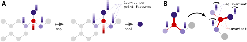
Figure 1: A) Each layer of the SE(3)-Transformer maps from a point cloud to a point cloud (or graph to graph) while guaranteeing equivariance. For classification, this is followed by an invariant pooling layer and an MLP. B) In each layer, for each node, attention is performed. Here, the red node attends to its neighbours. Attention weights (indicated by line thickness) are invariant w.r.t. input rotation.

Our contributions are the following:

• We introduce a novel self-attention mechanism, guaranteeably invariant to global rotations and translations of its input. It is also equivariant to permutations of the input point labels.

• We show that the SE(3)-Transformer resolves an issue with concurrent SE(3)-equivariant neural networks, which suffer from angularly constrained filters.

• We introduce a Pytorch implementation of spherical harmonics, which is 10x faster than Scipy on CPU and $100-1000\times$ faster on GPU. This directly addresses a bottleneck of TFNs [28]. E.g., for a ScanObjectNN model, we achieve $\approx 22\times$ speed up of the forward pass compared to a network built with SH from the lielearn library (see Appendix C).

• Code available at https://github.com/FabianFuchsML/se3-transformer-public

2 Background And Related Work

In this section we introduce the relevant background materials on self-attention, graph neural networks, and equivariance. We are concerned with point cloud based machine learning tasks, such as object classification or segmentation. In such a task, we are given a point cloud as input, represented as a collection of $n$ coordinate vectors $\textbf{x}_{i}\in\mathbb{R}^{3}$ with optional per-point features $\textbf{f}_{i}\in\mathbb{R}^{d}$.

2.1 The Attention Mechanism

The standard attention mechanism [31] can be thought of as consisting of three terms: a set of query vectors $\textbf{q}_{i}\in\mathbb{R}^{p}$ for $i=1,...,m$, a set of key vectors $\textbf{k}_{j}\in\mathbb{R}^{p}$ for $j=1,...,n$, and a set of value vectors $\textbf{v}_{j}\in\mathbb{R}^{r}$ for $j=1,...,n$, where $r$ and $p$ are the dimensions of the low dimensional embeddings. We commonly interpret the key $\textbf{k}_{j}$ and the value $\textbf{v}_{j}$ as being ‘attached’ to the same point $j$. For a given query $\textbf{q}_{i}$, the attention mechanism can be written as

$$\text{Attn}\left(\textbf{q}_{i},\{\textbf{k}_{j}\},\{\textbf{v}_{j}\}\right)=\sum_{j=1}^{n}\alpha_{ij}\textbf{v}_{j},\qquad\alpha_{ij}=\frac{\exp(\textbf{q}_{i}^{\top}\textbf{k}_{j})}{\sum_{j^{\prime}=1}^{n}\exp(\textbf{q}_{i}^{\top}\textbf{k}_{j^{\prime}})}$$ (1)

where we used a softmax as a nonlinearity acting on the weights. In general, the number of query vectors does not have to equal the number of input points [16]. In the case of self-attention the query, key, and value vectors are embeddings of the input features, so

$$\textbf{q}=h_{Q}(\textbf{f}), \textbf{k}=h_{K}(\textbf{f}), \textbf{v}=h_{V}(\textbf{f}),$$ (2)

where $\{h_{Q},h_{K},h_{V}\}$ are, in the most general case, neural networks [30]. For us, query $\textbf{q}_{i}$ is associated with a point $i$ in the input, which has a geometric location $\textbf{x}_{i}$. Thus if we have $n$ points, we have $n$ possible queries. For query $\textbf{q}_{i}$, we say that node $i$ attends to all other nodes $j\neq i$.

Motivated by a successes across a wide range of tasks in deep learning such as language modeling [31], image recognition [18], graph-based problems [32], and relational reasoning [30, 9], a recent stream of work has applied forms of self-attention algorithms to point cloud data [44, 42, 16]. One such example is the Set Transformer [16]. When applied to object classification on ModelNet40 [41], the input to the Set Transformer are the cartesian coordinates of the points. Each layer embeds this positional information further while dynamically querying information from other points. The final per-point embeddings are downsampled and used for object classification.

Permutation equivariance A key property of self-attention is permutation equivariance. Permutations of point labels $1,...,n$ lead to permutations of the self-attention output. This guarantees the attention output does not depend arbitrarily on input point ordering. Wagstaff et al. [33] recently showed that this mechanism can theoretically approximate all permutation equivariant functions. The SE(3)-transformer is a special case of this attention mechanism, inheriting permutation equivariance. However, it limits the space of learnable functions to rotation and translation equivariant ones.

2.2 Graph Neural Networks

Attention scales quadratically with point cloud size, so it is useful to introduce neighbourhoods: instead of each point attending to all other points, it only attends to its nearest neighbours. Sets with neighbourhoods are naturally represented as graphs. Attention has previously been introduced on graphs under the names of intra-, self-, vertex-, or graph-attention [17, 31, 32, 12, 26]. These methods were unified by Wang et al. [34] with the non-local neural network. This has the simple form

$$\textbf{y}_{i}=\frac{1}{\mathcal{C}(\{\textbf{f}_{j}\in\mathcal{N}_{i}\})}\sum_{j\in\mathcal{N}_{i}}w(\textbf{f}_{i},\textbf{f}_{j})h(\textbf{f}_{j})$$ (3)

where $w$ and $h$ are neural networks and $\mathcal{C}$ normalises the sum as a function of all features in the neighbourhood $\mathcal{N}_{i}$. This has a similar structure to attention, and indeed we can see it as performing attention per neighbourhood. While non-local modules do not explicitly incorporate edge-features, it is possible to add them, as done in Veličković et al. [32] and Hoshen [12].

2.3 Equivariance

Given a set of transformations $T_{g}:\mathcal{V}\to\mathcal{V}$ for $g\in G$, where $G$ is an abstract group, a function $\phi:\mathcal{V}\to\mathcal{Y}$ is called equivariant if for every $g$ there exists a transformation $S_{g}:\mathcal{Y}\to\mathcal{Y}$ such that

$$S_{g}[\phi(v)]=\phi(T_{g}[v])\qquad\text{for all }g\in G,v\in\mathcal{V}.$$ (4)

The indices $g$ can be considered as parameters describing the transformation. Given a pair $(T_{g},S_{g})$, we can solve for the family of equivariant functions $\phi$ satisfying Equation 4. Furthermore, if $(T_{g},S_{g})$ are linear and the map $\phi$ is also linear, then a very rich and developed theory already exists for finding $\phi$ [6]. In the equivariance literature, deep networks are built from interleaved linear maps $\phi$ and equivariant nonlinearities. In the case of 3D roto-translations it has already been shown that a suitable structure for $\phi$ is a tensor field network [28], explained below. Note that Romero et al. [24] recently introduced a 2D roto-translationally equivariant attention module for pixel-based image data.

Group Representations In general, the transformations $(T_{g},S_{g})$ are called group representations. Formally, a group representation $\rho:G\to GL(N)$ is a map from a group $G$ to the set of $N\times N$ invertible matrices $GL(N)$. Critically $\rho$ is a group homomorphism; that is, it satisfies the following property $\rho(g_{1}g_{2})=\rho(g_{1})\rho(g_{2})$ for all $g_{1},g_{2}\in G$. Specifically for 3D rotations $G=SO(3)$, we have a few interesting properties: 1) its representations are orthogonal matrices, 2) all representations can be decomposed as

$$\rho(g)=\textbf{Q}^{\top}\left[\bigoplus_{\ell}\textbf{D}_{\ell}(g)\right]\textbf{Q},$$ (5)

where Q is an orthogonal, $N\times N$, change-of-basis matrix [5]; each $\textbf{D}_{\ell}$ for $\ell=0,1,2,...$ is a $(2\ell+1)\times(2\ell+1)$ matrix known as a Wigner-D matrix; and the $\bigoplus$ is the direct sum or concatenation of matrices along the diagonal. The Wigner-D matrices are irreducible representations of SO(3)—think of them as the ‘smallest’ representations possible. Vectors transforming according to $\textbf{D}_{\ell}$ (i.e. we set $\textbf{Q}=\textbf{I}$), are called type-$\ell$ vectors. Type-0 vectors are invariant under rotations and type-1 vectors rotate according to 3D rotation matrices. Note, type-$\ell$ vectors have length $2\ell+1$. They can be stacked, forming a feature vector f transforming according to Eq. 5.

Tensor Field Networks Tensor field networks (TFN) [28] are neural networks, which map point clouds to point clouds under the constraint of SE(3)-equivariance, the group of 3D rotations and translations. For point clouds, the input is a vector field $\textbf{f}:\mathbb{R}^{3}\to\mathbb{R}^{d}$ of the form

$$\textbf{f}(\textbf{x})=\sum_{j=1}^{N}\textbf{f}_{j}\delta(\textbf{x}-\textbf{x}_{j}),$$ (6)

where $\delta$ is the Dirac delta function, $\{\textbf{x}_{j}\}$ are the 3D point coordinates and $\{\textbf{f}_{j}\}$ are point features, representing such quantities as atomic number or point identity. For equivariance to be satisfied, the features of a TFN transform under Eq. 5, where $\textbf{Q}=\textbf{I}$. Each $\textbf{f}_{j}$ is a concatenation of vectors of different types, where a subvector of type-$\ell$ is written $\textbf{f}_{j}^{\ell}$. A TFN layer computes the convolution of a continuous-in-space, learnable weight kernel $\textbf{W}^{\ell k}:\mathbb{R}^{3}\to\mathbb{R}^{(2\ell+1)\times(2k+1)}$ from type-$k$ features to type-$\ell$ features. The type-$\ell$ output of the TFN layer at position $\textbf{x}_{i}$ is

$$\textbf{f}_{\text{out},i}^{\ell}=\sum_{k\geq 0}\underbrace{\int\textbf{W}^{\ell k}(\textbf{x}^{\prime}-\textbf{x}_{i})\textbf{f}_{\text{in}}^{k}(\textbf{x}^{\prime})\,\mathrm{d}\textbf{x}^{\prime}}_{k\to\ell\text{ convolution}}=\sum_{k\geq 0}\sum_{j=1}^{n}\underbrace{\textbf{W}^{\ell k}(\textbf{x}_{j}-\textbf{x}_{i})\textbf{f}_{\text{in},j}^{k},}_{\text{node $j\to$ node $i$ message}}$$ (7)

We can also include a sum over input channels, but we omit it here. Weiler et al. [37], Thomas et al. [28] and Kondor [15] showed that the kernel $\textbf{W}^{\ell k}$ lies in the span of an equivariant basis $\{\textbf{W}_{J}^{\ell k}\}_{J=|k-\ell|}^{k+\ell}$. The kernel is a linear combination of these basis kernels, where the $J$^th coefficient is a learnable function $\varphi_{J}^{\ell k}:\mathbb{R}_{\geq 0}\to\mathbb{R}$ of the radius $\|\textbf{x}\|$. Mathematically this is

$$\textbf{W}^{\ell k}(\textbf{x})=\sum_{J=|k-\ell|}^{k+\ell}\varphi_{J}^{\ell k}(\|\textbf{x}\|)\textbf{W}_{J}^{\ell k}(\textbf{x}),\qquad\text{where }\textbf{W}_{J}^{\ell k}(\textbf{x})=\sum_{m=-J}^{J}Y_{Jm}(\textbf{x}/\|\textbf{x}\|)\textbf{Q}_{Jm}^{\ell k}.$$ (8)

Each basis kernel $\textbf{W}_{J}^{\ell k}:\mathbb{R}^{3}\to\mathbb{R}^{(2\ell+1)\times(2k+1)}$ is formed by taking a linear combination of Clebsch-Gordan matrices $\textbf{Q}_{Jm}^{\ell k}$ of shape $(2\ell+1)\times(2k+1)$, where the $J,m$^th linear combination coefficient is the $m$^th dimension of the $J$^th spherical harmonic $Y_{J}:\mathbb{R}^{3}\to\mathbb{R}^{2J+1}$. Each basis kernel $\textbf{W}_{J}^{\ell k}$ completely constrains the form of the learned kernel in the angular direction, leaving the only learnable degree of freedom in the radial direction. Note that $\textbf{W}_{J}^{\ell k}(\textbf{0})\neq\textbf{0}$ only when $k=\ell$ and $J=0$, which reduces the kernel to a scalar $w$ multiplied by the identity, $\textbf{W}^{\ell\ell}=w^{\ell\ell}\textbf{I}$, referred to as self-interaction [28]. As such we can rewrite the TFN layer as

$$\textbf{f}_{\text{out},i}^{\ell}=\underbrace{w^{\ell\ell}\textbf{f}_{\text{in},i}^{\ell}}_{\text{self-interaction}}+\sum_{k\geq 0}\sum_{j\neq i}^{n}\textbf{W}^{\ell k}(\textbf{x}_{j}-\textbf{x}_{i})\textbf{f}_{\text{in},j}^{k},$$ (9)

Eq. 7 and Eq. 9 present the convolution in message-passing form, where messages are aggregated from all nodes and feature types. They are also a form of nonlocal graph operation as in Eq. 3, where the weights are functions on edges and the features $\{\textbf{f}_{i}\}$ are node features. We will later see how our proposed attention layer unifies aspects of convolutions and graph neural networks.

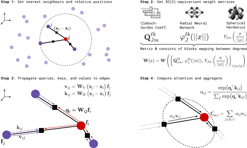
Figure 2: Updating the node features using our equivariant attention mechanism in four steps. A more detailed description, especially of step 2, is provided in the Appendix. Steps 3 and 4 visualise a graph network perspective: features are passed from nodes to edges to compute keys, queries and values, which depend both on features and relative positions in a rotation-equivariant manner.

3 Method

Here, we present the SE(3)-Transformer. The layer can be broken down into a procedure of steps as shown in Fig. 2, which we describe in the following section. These are the construction of a graph from a point cloud, the construction of equivariant edge functions on the graph, how to propagate SE(3)-equivariant messages on the graph, and how to aggregate them. We also introduce an alternative for the self-interaction layer, which we call attentive self-interaction.

3.1 Neighbourhoods

Given a point cloud $\{(\textbf{x}_{i},\textbf{f}_{i})\}$, we first introduce a collection of neighbourhoods $\mathcal{N}_{i}\subseteq\{1,...,N\}$, one centered on each point $i$. These neighbourhoods are computed either via the nearest-neighbours methods or may already be defined. For instance, molecular structures have neighbourhoods defined by their bonding structure. Neighbourhoods reduce the computational complexity of the attention mechanism from quadratic in the number of points to linear. The introduction of neighbourhoods converts our point cloud into a graph. This step is shown as Step 1 of Fig. 2.

3.2 The SE(3)-Transformer

The SE(3)-Transformer itself consists of three components. These are 1) edge-wise attention weights $\alpha_{ij}$, constructed to be SE(3)-invariant on each edge $ij$, 2) edge-wise SE(3)-equivariant value messages, propagating information between nodes, as found in the TFN convolution of Eq. 7, and 3) a linear/attentive self-interaction layer. Attention is performed on a per-neighbourhood basis as follows:

$$\textbf{f}_{\text{out},i}^{\ell}=\underbrace{\textbf{W}_{V}^{\ell\ell}\textbf{f}_{\text{in},i}^{\ell}}_{\text{ \raisebox{-0.9pt}{3}⃝ self-interaction}}+\sum_{k\geq 0}\sum_{j\in\mathcal{N}_{i}\setminus i}\underbrace{\alpha_{ij}}_{\text{\raisebox{-0.6pt}{1}⃝ attention}}\underbrace{\textbf{W}_{V}^{\ell k}(\textbf{x}_{j}-\textbf{x}_{i})\textbf{f}_{\text{in},j}^{k}}_{\text{\raisebox{-0.9pt}{2}⃝ value message}}.$$ (10)

These components are visualised in Fig. 2. If we remove the attention weights then we have a tensor field convolution, and if we instead remove the dependence of $\textbf{W}_{V}$ on $(\textbf{x}_{j}-\textbf{x}_{i})$, we have a conventional attention mechanism. Provided that the attention weights $\alpha_{ij}$ are invariant, Eq. 10 is equivariant to SE(3)-transformations. This is because it is just a linear combination of equivariant value messages. Invariant attention weights can be achieved with a dot-product attention structure shown in Eq. 11. This mechanism consists of a normalised inner product between a query vector $\textbf{q}_{i}$ at node $i$ and a set of key vectors $\{\textbf{k}_{ij}\}_{j\in\mathcal{N}_{i}}$ along each edge $ij$ in the neighbourhood $\mathcal{N}_{i}$ where

$$\alpha_{ij}=\frac{\exp(\textbf{q}_{i}^{\top}\textbf{k}_{ij})}{\sum_{j^{\prime}\in\mathcal{N}_{i}\setminus i}\exp(\textbf{q}_{i}^{\top}\textbf{k}_{ij^{\prime}})},\;\;\;\textbf{q}_{i}=\bigoplus_{\ell\geq 0}\sum_{k\geq 0}\textbf{W}_{Q}^{\ell k}\textbf{f}_{\text{in},i}^{k},\;\;\;\textbf{k}_{ij}=\bigoplus_{\ell\geq 0}\sum_{k\geq 0}\textbf{W}_{K}^{\ell k}(\textbf{x}_{j}-\textbf{x}_{i})\textbf{f}_{\text{in},j}^{k}.$$ (11)

$\bigoplus$ is the direct sum, i.e. vector concatenation in this instance. The linear embedding matrices $\textbf{W}_{Q}^{\ell k}$ and $\textbf{W}_{K}^{\ell k}(\textbf{x}_{j}-\textbf{x}_{i})$ are of TFN type (c.f. Eq. 8). The attention weights $\alpha_{ij}$ are invariant for the following reason. If the input features $\{\textbf{f}_{\text{in},j}\}$ are SO(3)-equivariant, then the query $\textbf{q}_{i}$ and key vectors $\{\textbf{k}_{ij}\}$ are also SE(3)-equivariant, since the linear embedding matrices are of TFN type. The inner product of SO(3)-equivariant vectors, transforming under the same representation $\textbf{S}_{g}$ is invariant, since if $\textbf{q}\mapsto\textbf{S}_{g}\textbf{q}$ and $\textbf{k}\mapsto\textbf{S}_{g}\textbf{k}$, then $\textbf{q}^{\top}\textbf{S}_{g}^{\top}\textbf{S}_{g}\textbf{k}=\textbf{q}^{\top}\textbf{k}$, because of the orthonormality of representations of SO(3), mentioned in the background section. We follow the common practice from the self-attention literature [31, 16], and chosen a softmax nonlinearity to normalise the attention weights to unity, but in general any nonlinear function could be used.

Aside: Angular Modulation The attention weights add extra degrees of freedom to the TFN kernel in the angular direction. This is seen when Eq. 10 is viewed as a convolution with a data-dependent kernel $\alpha_{ij}\textbf{W}_{V}^{\ell k}(\textbf{x})$. In the literature, SO(3) equivariant kernels are decomposed as a sum of products of learnable radial functions $\varphi_{J}^{\ell k}(\|\textbf{x}\|)$ and non-learnable angular kernels $\textbf{W}_{J}^{\ell k}(\textbf{x}/\|\textbf{x}\|)$ (c.f. Eq. 8). The fixed angular dependence of $\textbf{W}_{J}^{\ell k}(\textbf{x}/\|\textbf{x}\|)$ is a strange artifact of the equivariance condition in noncommutative algebras and while necessary to guarantee equivariance, it is seen as overconstraining the expressiveness of the kernels. Interestingly, the attention weights $\alpha_{ij}$ introduce a means to modulate the angular profile of $\textbf{W}_{J}^{\ell k}(\textbf{x}/\|\textbf{x}\|)$, while maintaining equivariance.

Channels, Self-interaction Layers, and Non-Linearities Analogous to conventional neural networks, the SE(3)-Transformer can straightforwardly be extended to multiple channels per representation degree $\ell$, so far omitted for brevity. This sets the stage for self-interaction layers. The attention layer (c.f. Fig. 2 and circles 1 and 2 of Eq. 10) aggregates information over nodes and input representation degrees $k$. In contrast, the self-interaction layer (c.f. circle 3 of Eq. 10) exchanges information solely between features of the same degree and within one node—much akin to 1x1 convolutions in CNNs. Self-interaction is an elegant form of learnable skip connection, transporting information from query point $i$ in layer $L$ to query point $i$ in layer $L+1$. This is crucial since, in the SE(3)-Transformer, points do not attend to themselves. In our experiments, we use two different types of self-interaction layer: (1) linear and (2) attentive, both of the form

$$\textbf{f}_{\text{out},i,c^{\prime}}^{\ell} =\sum_{c}w_{i,c^{\prime}c}^{\ell\ell}\textbf{f}_{\text{in},i,c}^{\ell}.$$ (12)

Linear: Following Schütt et al. [25], output channels are a learned linear combination of input channels using one set of weights $w_{i,c^{\prime}c}^{\ell\ell}=w_{c^{\prime}c}^{\ell\ell}$ per representation degree, shared across all points. As proposed in Thomas et al. [28], this is followed by a norm-based non-linearity.

Attentive: We propose an extension of linear self-interaction, attentive self-interaction, combining self-interaction and nonlinearity. We replace the learned scalar weights $w_{c^{\prime}c}^{\ell\ell}$ with attention weights output from an MLP, shown in Eq. 13 ($\bigoplus$ means concatenation.). These weights are SE(3)-invariant due to the invariance of inner products of features, transforming under the same representation.

$$w_{i,c^{\prime}c}^{\ell\ell}=\text{MLP}\left(\bigoplus_{c,c^{\prime}}\textbf{f}_{\text{in},i,c^{\prime}}^{\ell\top}\textbf{f}_{\text{in},i,c}^{\ell}\right)$$ (13)

3.3 Node and Edge Features

Point cloud data often has information attached to points (node-features) and connections between points (edge-features), which we would both like to pass as inputs into the first layer of the network. Node information can directly be incorporated via the tensors $\textbf{f}_{j}$ in Eqs. 6, LABEL: and 10. For incorporating edge information, note that $\textbf{f}_{j}$ is part of multiple neighbourhoods. One can replace $\textbf{f}_{j}$ with $\textbf{f}_{ij}$ in Eq. 10. Now, $\textbf{f}_{ij}$ can carry different information depending on which neighbourhood $\mathcal{N}_{i}$ we are currently performing attention over. In other words, $\textbf{f}_{ij}$ can carry information both about node $j$ but also about edge $ij$. Alternatively, if the edge information is scalar, it can be incorporated into the weight matrices $\textbf{W}_{V}$ and $\textbf{W}_{K}$ as an input to the radial network (see step 2 in Fig. 2).

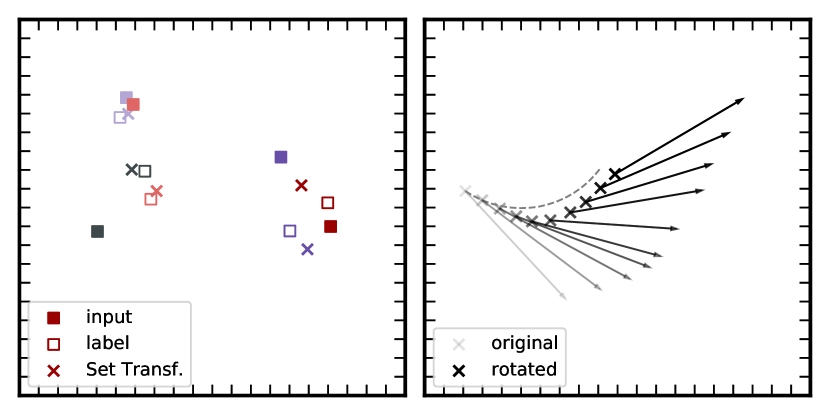
(a) Set Transformer

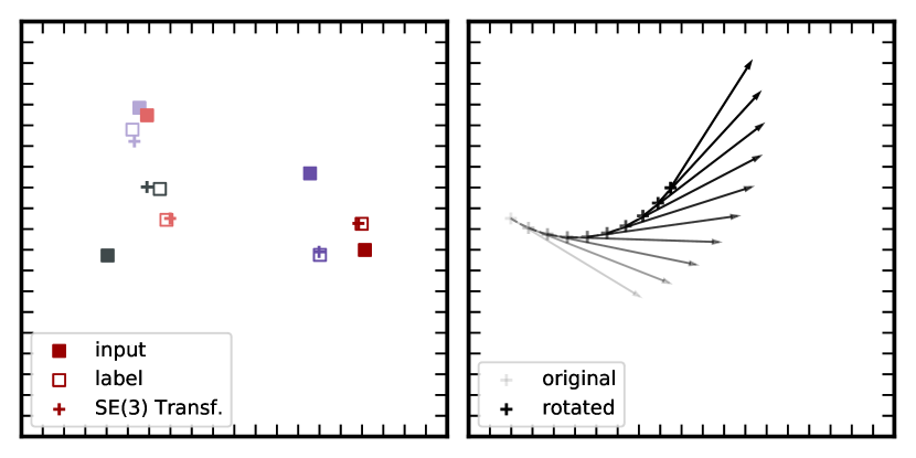
(b) SE(3)-Transformer

Figure 3: A model based on conventional self-attention (left) and our rotation-equivariant version (right) predict future locations and velocities in a 5-body problem. The respective left-hand plots show input locations at time step $t=0$, ground truth locations at $t=500$, and the respective predictions. The right-hand plots show predicted locations and velocities for rotations of the input in steps of 10 degrees. The dashed curves show the predicted locations of a perfectly equivariant model.

4 Experiments

We test the efficacy of the SE(3)-Transformer on three datasets, each testing different aspects of the model. The N-body problem is an equivariant task: rotation of the input should result in rotated predictions of locations and velocities of the particles. Next, we evaluate on a real-world object classification task. Here, the network is confronted with large point clouds of noisy data with symmetry only around the gravitational axis. Finally, we test the SE(3)-Transformer on a molecular property regression task, which shines light on its ability to incorporate rich graph structures. We compare to publicly available, state-of-the-art results as well as a set of our own baselines. Specifically, we compare to the Set-Transformer [16], a non-equivariant attention model, and Tensor Field Networks [28], which is similar to SE(3)-Transformer but does not leverage attention.

Similar to [27, 39], we measure the exactness of equivariance by applying uniformly sampled SO(3)-transformations to input and output. The distance between the two, averaged over samples, yields the equivariance error. Note that, unlike in Sosnovik et al. [27], the error is not squared:

$$\Delta_{EQ}=\left\|L_{s}\Phi(f)-\Phi L_{s}(f)\right\|_{2}/\left\|L_{s}\Phi(f)\|_{2}\right.$$ (14)

4.1 N-Body Simulations

In this experiment, we use an adaptation of the dataset from Kipf et al. [14]. Five particles each carry either a positive or a negative charge and exert repulsive or attractive forces on each other. The input to the network is the position of a particle in a specific time step, its velocity, and its charge. The task of the algorithm is then to predict the relative location and velocity 500 time steps into the future. We deliberately formulated this as a regression problem to avoid the need to predict multiple time steps iteratively. Even though it certainly is an interesting direction for future research to combine equivariant attention with, e.g., an LSTM, our goal here was to test our core contribution and compare it to related models. This task sets itself apart from the other two experiments by not being invariant but equivariant: When the input is rotated or translated, the output changes respectively (see Fig. 3).

We trained an SE(3)-Transformer with 4 equivariant layers, each followed by an attentive self-interaction layer (details are provided in the Appendix). Table 1 shows quantitative results. Our model outperforms both an attention-based, but not rotation-equivariant approach (Set Transformer) and a equivariant approach which does not levarage attention (Tensor Field). The equivariance error shows that our approach is indeed fully rotation equivariant up to the precision of the computations.

Table 1: Predicting future locations and velocities in an electron-proton simulation.

		Linear	DeepSet [46]	Tensor Field [28]	Set Transformer [16]	SE(3)-Transformer
	MSE $x$	$0.0691$	$0.0639$	$0.0151$	$0.0139$	$\bm{0.0076}$
Position	std	-	$0.0086$	$0.0011$	$0.0004$	$0.0002$
	$\Delta_{EQ}$	-	$0.038$	$1.9\cdot 10^{-7}$	$0.167$	$3.2\cdot 10^{-7}$
	MSE $v$	$0.261$	$0.246$	$0.125$	$0.101$	$\bm{0.075}$
Velocity	std	-	$0.017$	$0.002$	$0.004$	$0.001$
	$\Delta_{EQ}$	-	$1.11$	$5.0\cdot 10^{-7}$	$0.37$	$6.3\cdot 10^{-7}$

4.2 Real-World Object Classification on ScanObjectNN

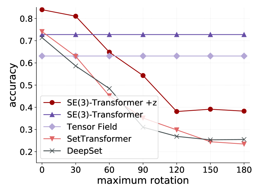
(a) Training without data augmentation.

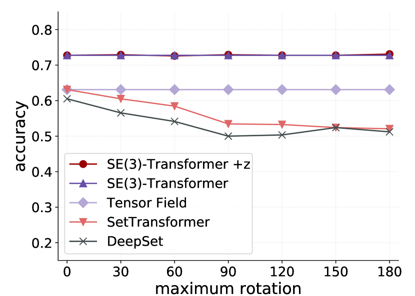
(b) Training with data augmentation.

Figure 4: ScanObjectNN: $x$-axis shows data augmentation on the test set. The $x$-value corresponds to the maximum rotation around a random axis in the $x$-$y$-plane. If both training and test set are not rotated ($x=0$ in a), breaking the symmetry of the SE(3)-Transformer by providing the $z$-component of the coordinates as an additional, scalar input improves the performance significantly. Interestingly, the model learns to ignore the additional, symmetry-breaking input when the training set presents a rotation-invariant problem (strongly overlapping dark red circles and dark purple triangles in b).

Object classification from point clouds is a well-studied task. Interestingly, the vast majority of current neural network methods work on scalar coordinates without incorporating vector specific inductive biases. Some recent works explore rotation invariant point cloud classification [45, 47, 4, 22]. Our method sets itself apart by using roto-translation equivariant layers acting directly on the point cloud without prior projection onto a sphere [22, 45, 7]. This allows for weight-tying and increased sample efficiency while transporting information about local and global orientation through the network - analogous to the translation equivariance of CNNs on 2D images. To test our method, we choose ScanObjectNN, a recently introduced dataset for real-world object classification. The benchmark provides point clouds of 2902 objects across 15 different categories. We only use the coordinates of the points as input and object categories as training labels. We train an SE(3)-Transformer with 4 equivariant layers with linear self-interaction followed by max-pooling and an MLP. Interestingly, the task is not fully rotation invariant, in a statistical sense, as the objects are aligned with respect to the gravity axis. This results in a performance loss when deploying a fully SO(3) invariant model (see Fig. 4(a)). In other words: when looking at a new object, it helps to know where ‘up’ is. We create an SO(2) invariant version of our algorithm by additionally feeding the $z$-component as an type-0 field and the $x$, $y$ position as an additional type-1 field (see Appendix). We dub this model SE(3)-Transformer +z. This way, the model can ‘learn’ which symmetries to adhere to by suppressing and promoting different inputs (compare Fig. 4(a) and Fig. 4(b)). In Table 2, we compare our model to the current state-of-the-art in object classification. Despite the dataset not playing to the strengths of our model (full SE(3)-invariance) and a much lower number of input points, the performance is competitive with models specifically designed for object classification - PointGLR [23], for instance, is pre-trained on the larger ModelNet40 dataset [41]. For a discussion of performance vs. number of input points used, see Section D.1.2.

Table 2: Classification accuracy on the ’object only’ category of the ScanObjectNN dataset⁴. The performance of the SE(3)-Transformer is averaged over 5 runs (standard deviation 0.7%).

	Tensor Field	DeepSet	SE(3)-Transf.	3DmFV	Set Transformer	PointNet	SpiderCNN	Tensor Field +z	PointNet++	SE(3)-Transf.+z	PointCNN	DGCNN	PointGLR
No. Points	128	1024	128	1024	1024	1024	1024	128	1024	128	1024	1024	1024
Accuracy	63.1%	71.4%	72.8 %	73.8%	74.1%	79.2%	79.5%	81.0%	84.3%	85.0%	85.5%	86.2%	87.2%

4.3 QM9

Table 3: QM9 Mean Absolute Error. Top: Non-equivariant models. Bottom: Equivariant models. SE(3)-Tr. is averaged over 5 runs.

Task	$\alpha$	$\Delta\varepsilon$	$\varepsilon_{\text{HOMO}}$	$\varepsilon_{\text{LUMO}}$	$\mu$	$C_{\nu}$
Units	$\text{bohr}^{3}$	meV	meV	meV	D	cal/mol K
WaveScatt [11]	.160	118	85	76	.340	.049
NMP [10]	.092	69	43	38	.030	.040
SchNet [25]	.235	63	41	34	.033	.033
Cormorant [1]	.085	61	34	38	.038	.026
LieConv(T3) [8]	.084	49	30	25	.032	.038
TFN [28]	.223	58	40	38	.064	.101
SE(3)-Transformer	.142$\pm$.002	53.0$\pm$0.3	35.0$\pm$.9	33.0$\pm$.7	.051$\pm$.001	.054$\pm$.002

The QM9 regression dataset [21] is a publicly available chemical property prediction task. There are 134k molecules with up to 29 atoms per molecule. Atoms are represented as a 5 dimensional one-hot node embeddings in a molecular graph connected by 4 different chemical bond types (more details in Appendix). ‘Positions’ of each atom are provided. We show results on the test set of Anderson et al. [1] for 6 regression tasks in Table 3. Lower is better. The table is split into non-equivariant (top) and equivariant models (bottom). Our nearest models are Cormorant and TFN (own implementation). We see that while not state-of-the-art, we offer competitive performance, especially against Cormorant and TFN, which transform under irreducible representations of SE(3) (like us), unlike LieConv(T3), using a left-regular representation of SE(3), which may explain its success.

5 Conclusion

We have presented an attention-based neural architecture designed specifically for point cloud data. This architecture is guaranteed to be robust to rotations and translations of the input, obviating the need for training time data augmentation and ensuring stability to arbitrary choices of coordinate frame. The use of self-attention allows for anisotropic, data-adaptive filters, while the use of neighbourhoods enables scalability to large point clouds. We have also introduced the interpretation of the attention mechanism as a data-dependent nonlinearity, adding to the list of equivariant nonlinearties which we can use in equivariant networks. Furthermore, we provide code for a speed up of spherical harmonics computation of up to 3 orders of magnitudes. This speed-up allowed us to train significantly larger versions of both the SE(3)-Transformer and the Tensor Field network [28] and to apply these models to real-world datasets.

Our experiments showed that adding attention to a roto-translation-equivariant model consistently led to higher accuracy and increased training stability. Specifically for large neighbourhoods, attention proved essential for model convergence. On the other hand, compared to convential attention, adding the equivariance constraints also increases performance in all of our experiments while at the same time providing a mathematical guarantee for robustness with respect to rotations of the input data.

Broader Impact

The main contribution of the paper is a mathematically motivated attention mechanism which can be used for deep learning on point cloud based problems. We do not see a direct potential of negative impact to the society. However, we would like to stress that this type of algorithm is inherently suited for classification and regression problems on molecules. The SE(3)-Transformer therefore lends itself to application in drug research. One concrete application we are currently investigating is to use the algorithm for early-stage suitability classification of molecules for inhibiting the reproductive cycle of the coronavirus. While research of this sort always requires intensive testing in wet labs, computer algorithms can be and are being used to filter out particularly promising compounds from large databases of millions of molecules.

Appendix A Group Theory and Tensor Field Networks

Groups

A group is an abstract mathematical concept. Formally a group $(G,\circ)$ consists of a set $G$ and a binary composition operator $\circ:G\times G\to G$ (typically we just use the symbol $G$ to refer to the group). All groups must adhere to the following 4 axioms

• Closure: $g\circ h\in G$ for all $g,h\in G$

• Associativity: $f\circ(g\circ h)=(f\circ g)\circ h=f\circ g\circ h$ for all $f,g,h\in G$

• Identity: There exists an element $e\in G$ such that $e\circ g=g\circ e=g$ for all $g\in G$

• Inverses: For each $g\in G$ there exists a $g^{-1}\in G$ such that $g^{-1}\circ g=g\circ g^{-1}=e$

In practice, we omit writing the binary composition operator $\circ$, so would write $gh$ instead of $g\circ h$. Groups can be finite or infinite, countable or uncountable, compact or non-compact. Note that they are not necessarily commutative; that is, $gh\neq hg$ in general.

Actions/Transformations

Groups are useful concepts, because they allow us to describe the structure of transformations, also sometimes called actions. A transformation (operator) $T_{g}:\mathcal{X}\to\mathcal{X}$ is an injective map from a space into itself. It is parameterised by an element $g$ of a group $G$. Transformations obey two laws:

• Closure: $T_{g}\circ T_{h}$ is a valid transformation for all $g,h\in G$

• Identity: There exists at least one element $e\in G$ such that $T_{e}[\textbf{x}]=\textbf{x}$ for all $\textbf{x}\in\mathcal{X}$,

where $\circ$ denotes composition of transformations. For the expression $T_{g}[\textbf{x}]$, we say that $T_{g}$ acts on x. It can also be shown that transformations are associative under composition. To codify the structure of a transformation, we note that due to closure we can always write

$$T_{g}\circ T_{h}=T_{gh},$$ (15)

If for any $x,y\in\mathcal{X}$ we can always find a group element $g$, such that $T_{g}[x]=y$, then we call $\mathcal{X}$ a homogeneous space. Homogeneous spaces are important concepts, because to each pair of points $x,y$ we can always associate at least one group element.

Equivariance and Intertwiners

As written in the main body of the text, equivariance is a property of functions $f:\mathcal{X}\to\mathcal{Y}$. Just to recap, given a set of transformations $T_{g}:\mathcal{X}\to\mathcal{X}$ for $g\in G$, where $G$ is an abstract group, a function $f:\mathcal{X}\to\mathcal{Y}$ is called equivariant if for every $g$ there exists a transformation $S_{g}:\mathcal{Y}\to\mathcal{Y}$ such that

$$S_{g}[f(\textbf{x})]=f(T_{g}[\textbf{x}])\qquad\text{for all }g\in G,\textbf{x}\in\mathcal{X}.$$ (16)

If $f$ is linear and equivariant, then it is called an intertwiner. Two important questions arise: 1) How do we choose $S_{g}$? 2) once we have $(T_{g},S_{g})$, how do we solve for $f$? To answer these questions, we need to understand what kinds of $S_{g}$ are possible. For this, we review representations.

Representations

A group representation $\rho:G\to GL(N)$ is a map from a group $G$ to the set of $N\times N$ invertible matrices $GL(N)$. Critically $\rho$ is a group homomorphism; that is, it satisfies the following property $\rho(g_{1}g_{2})=\rho(g_{1})\rho(g_{2})$ for all $g_{1},g_{2}\in G$. Representations can be used as transformation operators, acting on $N$-dimensional vectors $\textbf{x}\in\mathbb{R}^{N}$. For instance, for the group of 3D rotations, known as $SO(3)$, we have that 3D rotation matrices, $\rho(g)=\textbf{R}_{g}$ act on (i.e., rotate) 3D vectors, as

$$T_{g}[\textbf{x}]=\rho(g)\textbf{x}=\textbf{R}_{g}\textbf{x},\qquad\text{for all }\textbf{x}\in\mathcal{X},g\in G.$$ (17)

However, there are many more representations of $SO(3)$ than just the 3D rotation matrices. Among representations, two representations $\rho$ and $\rho^{\prime}$ of the same dimensionality are said to be equivalent if they can be connected by a similarity transformation

$$\rho^{\prime}(g)=\textbf{Q}^{-1}\rho(g)\textbf{Q},\qquad\text{for all }g\in G.$$ (18)

We also say that a representation is reducible if is can be written as

$$\rho(g)=\textbf{Q}^{-1}(\rho_{1}(g)\oplus\rho_{2}(g))\textbf{Q}=\textbf{Q}^{-1}\begin{bmatrix}\rho_{1}(g)&\\ &\rho_{2}(g)\end{bmatrix}\textbf{Q},\qquad\text{for all }g\in G.$$ (19)

If the representations $\rho_{1}$ and $\rho_{2}$ are not reducible, then they are called irreducible representations of $G$, or irreps. In a sense, they are the atoms among representations, out of which all other representations can be constructed. Note that each irrep acts on a separate subspace, mapping vectors from that space back into it. We say that subspace $\mathcal{X}_{\ell}\in\mathcal{X}$ is invariant under irrep $\rho_{\ell}$, if $\{\rho_{\ell}(g)\textbf{x}\,\,|\,\,\textbf{x}\in\mathcal{X}_{\ell},g\in G\}\subseteq\mathcal{X}_{\ell}$.

Representation theory of $SO(3)$

As it turns out, all linear representations of compact groups (such as $SO(3)$) can be decomposed into a direct sum of irreps, as

$$\rho(g)=\textbf{Q}^{\top}\left[\bigoplus_{J}\textbf{D}_{J}(g)\right]\textbf{Q},$$ (20)

where Q is an orthogonal, $N\times N$, change-of-basis matrix [5]; and each $\textbf{D}_{J}$ for $J=0,1,2,...$ is a $(2J+1)\times(2J+1)$ matrix known as a Wigner-D matrix. The Wigner-D matrices are the irreducible representations of $SO(3)$. We also mentioned that vectors transforming according to $\textbf{D}_{J}$ (i.e. we set $\textbf{Q}=\textbf{I}$), are called type-$J$ vectors. Type-0 vectors are invariant under rotations and type-1 vectors rotate according to 3D rotation matrices. Note, type-$J$ vectors have length $2J+1$. In the previous paragraph we mentioned that irreps act on orthogonal subspaces $\mathcal{X}_{0},\mathcal{X}_{1},...$. The orthogonal subspaces corresponding to the Wigner-D matrices are the space of spherical harmonics.

The Spherical Harmonics

The spherical harmonics $\textbf{Y}_{J}:S^{2}\to\mathbb{C}^{2J+1}$ for $J\geq 0$ are square-integrable complex-valued functions on the sphere $S^{2}$. They have the satisfying property that they are rotated directly by the Wigner-D matrices as

$$\textbf{Y}_{J}(\textbf{R}_{g}^{-1}\textbf{x})=\textbf{D}_{J}^{*}(g)\textbf{Y}_{J}(\textbf{x}),\qquad\textbf{x}\in S^{2},g\in G,$$ (21)

where $\textbf{D}_{J}$ is the $J$^th Wigner-D matrix and $\textbf{D}_{J}^{*}$ is its complex conjugate. They form an orthonormal basis for (the Hilbert space of) square-integrable functions on the sphere $L^{2}(S^{2})$, with inner product given as

$$\left\langle f,h\right\rangle_{S^{2}}=\int_{S^{2}}f(\textbf{x})h^{*}(\textbf{x})\,\mathrm{d}\textbf{x}.$$ (22)

So $\left\langle Y_{Jm},Y_{J^{\prime}m^{\prime}}\right\rangle_{S^{2}}=\delta_{JJ^{\prime}}\delta_{mm^{\prime}}$, where $Y_{Jm}$ is the $m$^th element of $\textbf{Y}_{J}$. We can express any function in $L^{2}(S^{2})$ as a linear combination of spherical harmonics, where

$$f(\textbf{x})=\sum_{J\geq 0}\textbf{f}_{J}^{\top}\textbf{Y}_{J}(\textbf{x}),\qquad\textbf{x}\in S^{2},$$ (23)

where each $\textbf{f}_{J}$ is a vector of coefficients of length $2J+1$. And in the opposite direction, we can retrieve the coefficients as

$$\textbf{f}_{J}=\int_{S^{2}}f(\textbf{x})\textbf{Y}_{J}^{*}(\textbf{x})\,\mathrm{d}\textbf{x}$$ (24)

following from the orthonormality of the spherical harmonics. This is in fact a Fourier transform on the sphere and the the vectors $\textbf{f}_{J}$ can be considered Fourier coefficients. Critically, we can represent rotated functions as

$$f(\textbf{R}_{g}^{-1}\textbf{x})=\sum_{J\geq 0}\textbf{f}_{J}^{\top}\textbf{D}_{J}^{*}(g)\textbf{Y}_{J}(\textbf{x}),\qquad\textbf{x}\in S^{2},g\in G.$$ (25)

The Clebsch-Gordan Decomposition

In the main text we introduced the Clebsch-Gordan coefficients. These are used in the construction of the equivariant kernels. They arise in the situation where we have a tensor product of Wigner-D matrices, which as we will see is part of the equivariance constraint on the form of the equivariant kernels. In representation theory a tensor product of representations is also a representation, but since it is not an easy object to work with, we seek to decompose it into a direct sum of irreps, which are easier. This decomposition is of the form of Eq. 20, written

$$\textbf{D}_{k}(g)\otimes\textbf{D}_{\ell}(g)=\textbf{Q}^{\ell k\top}\left[\bigoplus_{J=|k-\ell|}^{k+\ell}\textbf{D}_{J}(g)\right]\textbf{Q}^{\ell k}.$$ (26)

In this specific instance, the change of basis matrices $\textbf{Q}^{\ell k}$ are given the special name of the Clebsch-Gordan coefficients. These can be found in many mathematical physics libraries.

Tensor Field Layers

In Tensor Field Networks [28] and 3D Steerable CNNs [37], the authors solve for the intertwiners between SO(3) equivariant point clouds. Here we run through the derivation again in our own notation.

We begin with a point cloud $f(\textbf{x})=\sum_{j=1}^{N}\textbf{f}_{j}\delta(\textbf{x}-\textbf{x}_{j})$, where $\textbf{f}_{j}$ is an equivariant point feature. Let’s say that $\textbf{f}_{j}$ is a type-$k$ feature, which we write as $\textbf{f}_{j}^{k}$ to remind ourselves of the fact. Now say we perform a convolution $*$ with kernel $\textbf{W}^{\ell k}:\textbf{R}^{3}\to\mathbb{R}^{(2\ell+1)\times(2k+1)}$, which maps from type-$k$ features to type-$\ell$ features. Then

$$\textbf{f}_{\text{out,i}}^{\ell} =[\textbf{W}^{\ell k}*\textbf{f}_{\text{in}}^{k}](\textbf{x})$$ (27)

$$=\int_{\mathbb{R}^{3}}\textbf{W}^{\ell k}(\textbf{x}^{\prime}-\textbf{x}_{i})\textbf{f}_{\text{in}}^{k}(\textbf{x}^{\prime})\,\mathrm{d}\textbf{x}^{\prime}$$ (28)

$$=\int_{\mathbb{R}^{3}}\textbf{W}^{\ell k}(\textbf{x}^{\prime}-\textbf{x}_{i})\sum_{j=1}^{N}\textbf{f}_{\text{in},j}^{k}\delta(\textbf{x}^{\prime}-\textbf{x}_{j})\,\mathrm{d}\textbf{x}^{\prime}$$ (29)

$$=\sum_{j=1}^{N}\int_{\mathbb{R}^{3}}\textbf{W}^{\ell k}(\textbf{x}^{\prime}-\textbf{x}_{i})\textbf{f}_{\text{in},j}^{k}\delta(\textbf{x}^{\prime}-\textbf{x}_{j})\,\mathrm{d}\textbf{x}^{\prime} \text{change of variables }\textbf{x}^{\prime\prime}=\textbf{x}^{\prime}-\textbf{x}_{j}$$ (30)

$$=\sum_{j=1}^{N}\int_{\mathbb{R}^{3}}\textbf{W}^{\ell k}(\textbf{x}^{\prime\prime}+\textbf{x}_{j}-\textbf{x}_{i})\textbf{f}_{\text{in},j}^{k}\delta(\textbf{x}^{\prime\prime})\,\mathrm{d}\textbf{x}^{\prime\prime}$$ sifting theorem (31)

$$=\sum_{j=1}^{N}\textbf{W}^{\ell k}(\textbf{x}_{j}-\textbf{x}_{i})\textbf{f}_{\text{in},j}^{k}.$$ (32)

Now let’s apply the equivariance condition to this expression, then

$$\textbf{D}_{\ell}(g)\textbf{f}_{\text{out,i}}^{\ell} =\sum_{j=1}^{N}\textbf{W}^{\ell k}(\textbf{R}_{g}^{-1}(\textbf{x}_{j}-\textbf{x}_{i}))\textbf{D}_{k}(g)\textbf{f}_{\text{in},j}^{k}$$ (33)

$$\implies\textbf{f}_{\text{out,i}}^{\ell} =\sum_{j=1}^{N}\textbf{D}_{\ell}(g)^{-1}\textbf{W}^{\ell k}(\textbf{R}_{g}^{-1}(\textbf{x}_{j}-\textbf{x}_{i}))\textbf{D}_{k}(g)\textbf{f}_{\text{in},j}^{k}$$ (34)

Now we notice that this expression should also be equal to Eq. 32, which is the convolution with an unrotated point cloud. Thus we end up at

$$\boxed{\textbf{W}^{\ell k}(\textbf{R}_{g}^{-1}\textbf{x})=\textbf{D}_{\ell}(g)\textbf{W}^{\ell k}(\textbf{x})\textbf{D}_{k}(g)^{-1},}$$ (35)

which is sometimes refered to as the kernel constraint. To solve the kernel constraint, we notice that it is a linear equation and that we can rearrange it as

$$\text{vec}(\textbf{W}^{\ell k}(\textbf{R}_{g}^{-1}\textbf{x}))=(\textbf{D}_{k}(g)\otimes\textbf{D}_{\ell}(g))\text{vec}(\textbf{W}^{\ell k}(\textbf{x}))$$ (36)

where we used the identity $\text{vec}(\textbf{AXB})=(\textbf{B}^{\top}\otimes\textbf{A})\text{vec}(\textbf{X})$ and the fact that the Wigner-D matrices are orthogonal. Using the Clebsch-Gordan decomposition we rewrite this as

$$\text{vec}(\textbf{W}^{\ell k}(\textbf{R}_{g}^{-1}\textbf{x}))=\textbf{Q}^{\ell k\top}\left[\bigoplus_{J=|k-\ell|}^{k+\ell}\textbf{D}_{J}(g)\right]\textbf{Q}^{\ell k}\text{vec}(\textbf{W}^{\ell k}(\textbf{R}_{g}^{-1}\textbf{x})).$$ (37)

Lastly, we can left multiply both sides by $\textbf{Q}^{\ell k}$ and denote $\bm{\eta}^{\ell k}(\textbf{x})\triangleq\textbf{Q}^{\ell k}\text{vec}(\textbf{W}^{\ell k}(\textbf{x}))$, noting the the Clebsch-Gordan matrices are orthogonal. At the same time we

$$\bm{\eta}^{\ell k}(\textbf{R}_{g}^{-1}\textbf{x})=\left[\bigoplus_{J=|k-\ell|}^{k+\ell}\textbf{D}_{J}(g)\right]\bm{\eta}^{\ell k}(\textbf{x}).$$ (38)

Thus we have that $\bm{\eta}^{\ell k}_{J}(\textbf{R}_{g}^{-1}\textbf{x})$ the $J$^th subvector of $\bm{\eta}^{\ell k}(\textbf{R}_{g}^{-1}\textbf{x})$ is subject to the constraint

$$\bm{\eta}_{J}^{\ell k}(\textbf{R}_{g}^{-1}\textbf{x})=\textbf{D}_{J}(g)\bm{\eta}_{J}^{\ell k}(\textbf{x}),$$ (39)

which is exactly the transformation law for the spherical harmonics from Eq. 21! Thus one way how $\textbf{W}^{\ell k}(\textbf{x})$ can be constructed is

$$\text{vec}\left(\textbf{W}^{\ell k}(\textbf{x})\right)=\textbf{Q}^{\ell k\top}\bigoplus_{J=|k-\ell|}^{k+\ell}\textbf{Y}_{J}(\textbf{x}).$$ (40)

Appendix B Recipe for Building an Equivariant Weight Matrix

One of the core operations in the SE(3)-Transformer is multiplying a feature vector f, which transforms according to $SO(3)$, with a matrix W while preserving equivariance:

$$S_{g}[\textbf{W}*\textbf{f}](\textbf{x})=[\textbf{W}*T_{g}[\textbf{f}]](\textbf{x}),$$ (41)

where $T_{g}[\textbf{f}](\textbf{x})=\rho_{\text{in}}(g)\textbf{f}(\textbf{R}_{g}^{-1}\textbf{x})$ and $S_{g}[\textbf{f}](\textbf{x})=\rho_{\text{out}}(g)\textbf{f}(\textbf{R}_{g}^{-1}\textbf{x})$. Here, as in the previous section we showed how such a matrix W could be constructed when mapping between features of type-$k$ and type-$\ell$, where $\rho_{\text{in}}(g)$ is a block diagonal matrix of type-$k$ Wigner-D matrices and similarly $\rho_{\text{in}}(g)$ is made of type-$\ell$ Wigner-D matrices. W is dependent on the relative position x and underlies the linear equivariance constraints, but is also has learnable components, which we did not show in the previous section. In this section, we show how such a matrix is constructed in practice.

Previously we showed that

$$\text{vec}\left(\textbf{W}^{\ell k}(\textbf{x})\right)=\textbf{Q}^{\ell k\top}\bigoplus_{J=|k-\ell|}^{k+\ell}\textbf{Y}_{J}(\textbf{x}),$$ (42)

which is an equivariant mapping between vectors of types $k$ and $\ell$. In practice, we have multiple input vectors $\{\textbf{f}_{c}^{k}\}_{c}$ of type-$k$ and multiple output vectors of type-$\ell$. For simplicity, however, we ignore this and pretend we only have a single input and single output. Note that $\textbf{W}^{\ell k}$ has no learnable components. Note that the kernel constraint only acts in the angular direction, but not in the radial direction, so we can introduce scalar radial functions $\varphi_{J}^{\ell k}:\textbf{R}_{\geq 0}\to\textbf{R}$ (one for each $J$), such that

$$\text{vec}\left(\textbf{W}^{\ell k}(\textbf{x})\right)=\textbf{Q}^{\ell k\top}\bigoplus_{J=|k-\ell|}^{k+\ell}\varphi_{J}^{\ell k}(\|\textbf{x}\|)\textbf{Y}_{J}(\textbf{x}),$$ (43)

The radial functions $\varphi_{J}^{\ell k}(\|\textbf{x}\|)$ act as an independent, learnable scalar factor for each degree $J$. The vectorised matrix has dimensionality $(2\ell+1)(2k+1)$. We can unvectorise the above yielding

$$\textbf{W}^{\ell k}(\textbf{x}) =\text{unvec}\left(\textbf{Q}^{\ell k\top}\bigoplus_{J=|k-\ell|}^{k+\ell}\varphi_{J}^{\ell k}(\|\textbf{x}\|)\textbf{Y}_{J}(\textbf{x})\right)$$ (44)

$$=\sum_{J=|k-\ell|}^{k+\ell}\varphi_{J}^{\ell k}(\|\textbf{x}\|)\text{unvec}\left(\textbf{Q}_{J}^{\ell k\top}\textbf{Y}_{J}(\textbf{x})\right)$$ (45)

where $\textbf{Q}_{J}^{\ell k}$ is a $(2\ell+1)(2k+1)\times(2J+1)$ slice from $\textbf{Q}^{\ell k}$, corresponding to spherical harmonic $\textbf{Y}_{J}.$ As we showed in the main text, we can also rewrite the unvectorised Clebsch-Gordan–spherical harmonic matrix-vector product as

$$\text{unvec}\left(\textbf{Q}_{J}^{\ell k\top}\textbf{Y}_{J}(\textbf{x})\right)=\sum_{m=-J}^{J}\textbf{Q}_{Jm}^{\ell k\top}Y_{Jm}(\textbf{x}).$$ (46)

In contrast to Weiler et al. [37], we do not voxelise space and therefore x will be different for each pair of points in each point cloud. However, the same $\textbf{Y}_{J}\left(\textbf{x}\right)$ will be used multiple times in the network and even multiple times in the same layer. Hence, precomputing them at the beginning of each forward pass for the entire network can significantly speed up the computation. The Clebsch-Gordan coefficients do not depend on the relative positions and can therefore be precomputed once and stored on disk. Multiple libraries exist which approximate those coefficients numerically.

Appendix C Accelerated Computation of Spherical Harmonics

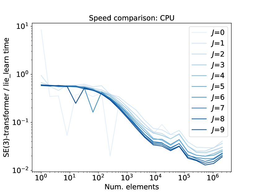
(a) Speed comparison on the CPU.

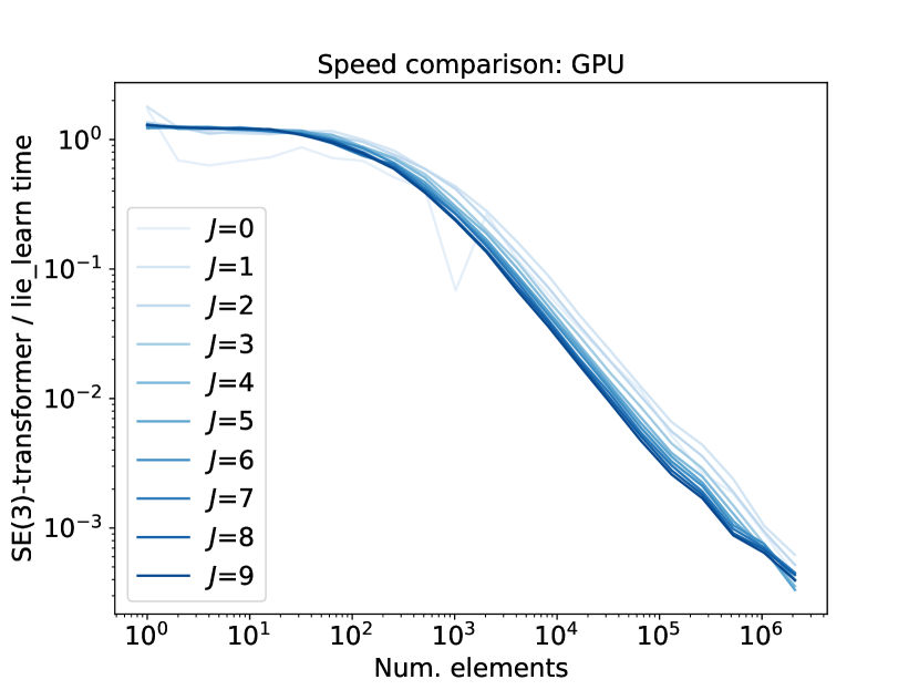
(b) Speed comparison on the GPU.

Figure 5: Spherical harmonics computation of our own implementation compared to the lie-learn library. We found that speeding up the computation of spherical harmonics is critical to scale up both Tensor Field Networks [28] and SE(3)-Transformers to solve real-world machine learning tasks.

The spherical harmonics (SH) typically have to be computed on the fly for point cloud methods based on irreducible computations, a bottleneck of TFNs [28]. Thomas et al. [28] ameliorate this by restricting the maximum type of feature to type-2, trading expressivity for speed. Weiler et al. [37] circumvent this challenge by voxelising the input, allowing them to pre-compute spherical harmonics for fixed relative positions. This is at the cost of detail as well as exact rotation and translation equivariance.

The number of spherical harmonic lookups in a network based on irreducible representations can quickly become large (number of layers $\times$ number of points $\times$ number of neighbours $\times$ number of channels $\times$ number of degrees needed). This motivates parallelised computation on the GPU - a feature not supported by common libraries. To that end, we wrote our own spherical harmonics library in Pytorch, which can generate spherical harmonics on the GPU. We found this critical to being able to run the SE(3)-Transformer and Tensor Field network baselines in a reasonable time. This library is accurate to within machine precision against the scipy counterpart scipy.special.sph_harm and is significantly faster. E.g., for a ScanObjectNN model, we achieve $\sim 22\times$ speed up of the forward pass compared to a network built with SH from the lielearn library. A speed comparison isolating the computation of the spherical harmonics is shown in Fig. 5. Code is available at https://github.com/FabianFuchsML/se3-transformer-public. In the following, we outline our method to generate them.

The tesseral/real spherical harmonics are given as

$$Y_{Jm}(\theta,\phi)=\sqrt{\frac{2J+1}{4\pi}\frac{(J-m)!}{(J+m)!}}P_{J}^{|m|}(\cos\theta)\cdot\left\{\begin{matrix}[l]\sin(|m|\phi)&m<0,\\ 1&m=0,\\ \cos(m\phi)&m>0,\end{matrix}\right.$$ (47)

where $P_{J}^{|m|}$ is the associated Legendre polynomial (ALP), $\theta\in[0,2\pi)$ is azimuth, and $\phi\in[0,\pi]$ is a polar angle. The term $P_{J}^{|m|}$ is by far the most expensive component to compute and can be computed recursively. To speed up the computation, we use dynamic programming storing intermediate results in a memoization.

We make use of the following recursion relations in the computation of the ALPs:

$$P_{J}^{|J|}(x) =(-1)^{|J|}\cdot(1-x^{2})^{|J|/2}\cdot(2|J|-1)!! J=m$$ boundary: (48)

$$P_{J}^{-m}(x) =(-1)^{J}\frac{(\ell-m)!}{(\ell+m)!}P_{J}^{m}(x) m$$ negate (49)

$$P_{J}^{|m|}(x) =\frac{2J-1}{J-|m|}xP_{J-1}^{m}(x)+\mathbb{I}[J-|m|>1]\frac{J+|m|-1}{J-|m|}P_{J-2}^{m}(x)$$ recurse (50)

where the semifactorial is defined as $x!!=x(x-2)(x-4)\cdots$, and $\mathbb{I}$ is the indicator function. These relations are helpful because they define a recursion.

To understand how we recurse, we consider an example. Fig. 6 shows the space of $J$ and $m$. The black vertices represent a particular ALP, for instance, we have highlighted $P_{3}^{-1}(x)$. When $m<0$, we can use Eq. 49 to compute $P_{3}^{-1}(x)$ from $P_{3}^{1}(x)$. We can then use Eq. 50 to compute $P_{3}^{1}(x)$ from $P_{2}^{1}(x)$ and $P_{1}^{1}(x)$. $P_{2}^{1}(x)$ can also be computed from Eq. 50 and the boundary value $P_{1}^{1}(x)$ can be computed directly using Eq. 48. Crucially, all intermediate ALPs are stored for reuse. Say we wanted to compute $P_{4}^{-1}(x)$, then we could use Eq. 49 to find it from $P_{4}^{-1}(x)$, which can be recursed from the stored values $P_{3}^{1}(x)$ and $P_{2}^{1}(x)$, without needing to recurse down to the boundary.

Figure 6: Subproblem graph for the computatin of the associated Legendre polynomials. To compute $P_{3}^{-1}(x)$, we compute $P_{3}^{1}(x)$, for which we need $P_{2}^{1}(x)$ and $P_{1}^{1}(x)$. We store each intermediate computation, speeding up average computation time by a factor of $\sim 10$ on CPU.

Appendix D Experimental Details

D.1 ScanObjectNN

D.1.1 SE(3)-Transformer and Tensor Field Network

A particularity of object classification from point clouds is the large number of points the algorithm needs to handle. We use up to 200 points out of the available 2024 points per sample and create neighbourhoods with up to 40 nearest neighbours. It is worth pointing out that especially in this setting, adding self-attention (i.e. when comparing the SE(3) Transformer to Tensor Field Networks) significantly increased the stability. As a result, whenever we swapped out the attention mechanism for a convolution to retrieve the Tensor Field network baseline, we had to decrease the model size to obtain stable training. However, we would like to stress that all the Tensor Field networks we trained were significantly bigger than in the original paper [28], mostly enabled by the faster computation of the spherical harmonics.

For the ablation study in Fig. 4, we trained networks with 4 hidden equivariant layers with 5 channels each, and up to representation degree 2. This results in a hidden feature size per point of

$$5\cdot\sum_{\ell=0}^{2}(2\ell+1)=45$$ (51)

We used 200 points of the point cloud and neighbourhood size 40. For the Tensor Field network baseline, in order to achieve stable training, we used a smaller model with 3 instead of 5 channels, 100 input points and neighbourhood size 10, but with representation degrees up to 3.

We used 1 head per attention mechanism yielding one attention weight for each pair of points but across all channels and degrees (for an implementation of multi-head attention, see Section D.3). For the query embedding, we used the identity matrix. For the key embedding, we used a square equivariant matrix preserving the number of degrees and channels per degree.

For the quantitative comparison to the start-of-the-art in Table 2, we used 128 input points and neighbourhood size 10 for both the Tensor Field network baseline and the SE(3)-Transformer. We used farthest point sampling with a random starting point to retrieve the 128 points from the overall point cloud. We used degrees up to 3 and 5 channels per degree, which we again had to reduce to 3 channels for the Tensor Field network to obtain stable training. We used a norm based non-linearity for the Tensor Field network (as in [28]) and no extra non-linearity (beyond the softmax in the self-attention algorithm) for the SE(3) Transformer.

For all experiments, the final layer of the equivariant encoder maps to 64 channels of degree 0 representations. This yields a 64-dimensional SE(3) invariant representation per point. Next, we pool over the point dimension followed by an MLP with one hidden layer of dimension 64, a ReLU and a 15 dimensional output with a cross entropy loss. We trained for 60000 steps with batch size 10. We used the Adam optimizer [13] with a start learning of 1e-2 and a reduction of the learning rate by 70% every 15000 steps. Training took up to 2 days on a system with 4 CPU cores, 30 GB of RAM, and an NVIDIA GeForce GTX 1080 Ti GPU.

The input to the Tensorfield network and the Se(3) Transformer are relative x-y-z positions of each point w.r.t. their neighbours. To guarantee equivariance, these inputs are provided as fields of degree 1. For the ‘+z‘ versions, however, we deliberately break the SE(3) equivariance by providing additional and relative z-position as two additional scalar fields (i.e. degree 0), as well as relative x-y positions as a degree 1 field (where the z-component is set to 0).

D.1.2 Number of Input Points

Limiting the input to 128/200 points in our experiments on ScanObjectNN was not primarily due to computational limitations: we conducted experiments with up to 2048 points, but without performance improvements. We suspect this is due to the global pooling. Examining cascaded pooling via attention is a future research direction. Interestingly, when limiting other methods to using 128 points, the SE(3)-Transformer outperforms the baselines (PointCNN: $80.3\pm 0.8\%$, PointGLR: $81.5\pm 1.0\%$, DGCNN: $82.2\pm 0.8\%$, ours: $85.0\pm 0.7\%$). It is worth noting that these methods were explicitly designed for the well-studied task of point classification whereas the SE(3)-Transformer was applied as is. Combining different elements from the current state-of-the-art methods with the geometrical inductive bias of the SE(3)-Transformer could potentially yield additional performance gains, especially with respect to leveraging inputs with more points. It is also worth noting that the SE(3)-Transformer was remarkably stable with respect to lowering the number of input points in an ablation study (16 points: $79.2\%$, 32 points: $81.4\%$, 64 points: $82.5\%$, 128 points: $85.0\%$, 256 points: $82.6\%$).

D.1.3 Sample Complexity

Equivariance is known to often lead to smaller sample complexity, meaning that less training data is needed (Fig. 10 in Worrall et al. [40], Fig. 4 in Winkels and Cohen [38], Fig. 4 in Weiler et al. [37]). We conducted experiments with different amounts of training samples $N_{\text{samples}}$ from the ScanObjectNN dataset. The results showed that for all $N_{\text{samples}}$, the SE(3)-Transformer outperformed the Set Transformer, a non-equivariant network based on attention. The performance delta was also slightly higher for the smallest $N_{\text{samples}}$ we tested ($3.1\%$ of the samples available in the training split of ScanObjectNN) than when using all the data indicating that the SE(3)-Transformer performs particularly well on small amounts of training data. However, performance differences can be due to multiple reasons. Especially for small datasets, such as ScanObjectNN, where the performance does not saturate with respect to amount of data available, it is difficult to draw conclusions about sample complexity of one model versus another. In summary, we found that our experimental results are in line with the claim that equivariance decreases sample complexity in this specific case but do not give definitive support.

D.1.4 Baselines

DeepSet Baseline

We originally replicated the implementation proposed in [46] for their object classification experiment on ModelNet40 [41]. However, most likely due to the relatively small number of objects in the ScanObjectNN dataset, we found that reducing the model size helped the performance significantly. The reported model had 128 units per hidden layer (instead of 256) and no dropout but the same number of layers and type of non-linearity as in [46].

Set Transformer Baseline

We used the same architecture as [16] in their object classification experiment on ModelNet40 [41] with an ISAB (induced set attention block)-based encoder followed by PMA (pooling by multihead attention) and an MLP.

D.2 Relational Inference

Following Kipf et al. [14], we simulated trajectories for $5$ charged, interacting particles. Instead of a 2d simulation setup, we considered a 3d setup. Positive and negative charges were drawn as Bernoulli trials ($p=0.5$). We used the provided code base https://github.com/ethanfetaya/nri with the following modifications: While we randomly sampled initial positions inside a $[-5,5]^{3}$ box, we removed the bounding-boxes during the simulation. We generated $5\text{k}$ simulation samples for training and $1\text{k}$ for testing. Instead of phrasing it as a time-series task, we posed it as a regression task: The input data is positions and velocities at a random time step as well as the signs of the charges. The labels (which the algorithm is learning to predict) are the positions and velocities 500 simulation time steps into the future.

Training Details

We trained each model for 100,000 steps with batch size 128 using an Adam optimizer [13]. We used a fixed learning rate throughout training and conducted a separate hyper parameter search for each model to find a suitable learning rate.

SE(3)-Transformer Architecture

We trained an SE(3)-Transformer with 4 equivariant layers, where the hidden layers had representation degrees $\{0,1,2,3\}$ and 3 channels per degree. The input is handled as two type-1 fields (for positions and velocities) and one type-0 field (for charges). The learning rate was set to 3e-3. Each layer included attentive self-interaction.

We used 1 head per attention mechanism yielding one attention weight for each pair of points but across all channels and degrees (for an implementation of multi-head attention, see Section D.3). For the query embedding, we used the identity matrix. For the key embedding, we used a square equivariant matrix preserving the number of degrees and channels per degree.

Baseline Architectures

All our baselines fulfill permutation invariance (ordering of input points), but only the Tensor Field network and the linear baseline are SE(3) equivariant. For the Tensor Field Network[28] baseline, we used the same hyper parameters as for the SE(3) Transformer but with a linear self-interaction and an additional norm-based nonlinearity in each layer as in Thomas et al. [28]. For the DeepSet[46] baseline, we used 3 fully connected layers, a pooling layer, and two more fully connected layers with 64 units each. All fully connected layers act pointwise. The pooling layer uses max pooling to aggregate information from all points, but concatenates this with a skip connection for each point. Each hidden layer was followed by a LeakyReLU. The learning rate was set to 1e-3. For the Set Transformer[16], we used 4 self-attention blocks with 64 hidden units and 4 heads each. For each point this was then followed by a fully connected layer (64 units), a LeakyReLU and another fully connected layer. The learning rate was set to 3e-4.

For the linear baseline, we simply propagated the particles linearly according to the simulation hyperparamaters. The linear baseline can be seen as removing the interactions between particles from the prediction. Any performance improvement beyond the linear baseline can therefore be interpreted as an indication for relational reasoning being performed.

D.3 QM9

The QM9 regression dataset [21] is a publicly available chemical property prediction task consisting of 134k small drug-like organic molecules with up to 29 atoms per molecule. There are 5 atomic species (Hydrogen, Carbon, Oxygen, Nitrogen, and Flourine) in a molecular graph connected by chemical bonds of 4 types (single, double, triple, and aromatic bonds). ‘Positions’ of each atom, measured in ångtröms, are provided. We used the exact same train/validation/test splits as Anderson et al. [1] of sizes 100k/18k/13k.

The architecture we used is shown in Table 4. It consists of 7 multihead attention layers interspersed with norm nonlinearities, followed by a TFN layer, max pooling, and two linear layers separated by a ReLU. For each attention layer, shown in Fig. 7, we embed the input to half the number of feature channels before applying multiheaded attention [31]. Multiheaded attention is a variation of attention, where we partition the queries, keys, and values into $H$ attention heads. So if our embeddings have dimensionality $(4,16)$ (denoting 4 feature types with 16 channels each) and we use $H=8$ attention heads, then we partition the embeddings to shape $(4,2)$. We then combine each of the 8 sets of shape $(4,2)$ queries, keys, and values individually and then concatenate the results into a single vector of the original shape $(4,16)$. The keys and queries are edge embeddings, and thus the embedding matrices are of TFN type (c.f. Eq. 8). For TFN type layers, the radial functions are learnable maps. For these we used neural networks with architecture shown in Table 5.

For the norm nonlinearities [40], we use

$$\texttt{Norm ReLU}(\textbf{f}^{\ell})=\texttt{ReLU}(\texttt{LN}\left(\|\textbf{f}^{\ell}\|\right))\cdot\frac{\textbf{f}^{\ell}}{\|\textbf{f}^{\ell}\|},\qquad\text{where }\|\textbf{f}^{\ell}\|=\sqrt{\sum_{m=-\ell}^{\ell}(f_{m}^{\ell})^{2}},$$ (52)

where LN is layer norm [2] applied across all features within a feature type. For the TFN baseline, we used the exact same architecture but we replaced each of the multiheaded attention blocks with a TFN layer with the same output shape.

The input to the network is a sparse molecular graph, with edges represented by the molecular bonds. The node embeedings are a 6 dimensional vector composed of a 5 dimensional one-hot embedding of the 5 atomic species and a 1 dimension integer node embedding for number of protons per atom. The edges embeddings are a 5 dimensional vector consisting of a 4 dimensional one-hot embedding of bond type and a positive scalar for the Euclidean distance between the two atoms at the ends of the bond. For each regression target, we normalised the values by mean and dividing by the standard deviation of the training set.

We trained for 50 epochs using Adam [13] at initial learning rate 1e-3 and a single-cycle cosine rate-decay to learning rate 1e-4. The batch size was 32, but for the TFN baseline we used batch size 16, to fit the model in memory. We show results on the 6 regression tasks not requiring thermochemical energy subtraction in Table 3. As is common practice, we optimised architectures and hyperparameters on $\varepsilon_{\text{HOMO}}$ and retrained each network on the other tasks. Training took about 2.5 days on an NVIDIA GeForce GTX 1080 Ti GPU with 4 CPU cores and 15 GB of RAM.

Table 4: QM9 Network architecture: $d_{\text{out}}$ is the number of feature types of degrees $0,1,...,d_{\text{out}}-1$ at the output of the corresponding layer and $C$ is the number of multiplicities/channels per feature type. For the norm nonlinearity we use ReLUs, preceded by equivariant layer norm [37] with learnable affine transform.

No. repeats	Layer Type	$d_{\text{out}}$	$C$
1x	Input	1	6
1x	Attention: 8 heads	4	16
	Norm Nonlinearity	4	16
6x	Attention: 8 heads	4	16
	Norm Nonlinearity	4	16
1x	TFN layer	1	128
1x	Max pool	1	128
1x	Linear	1	128
1x	ReLU	1	128
1x	Linear	1	1

Table 5: QM9 Radial Function Architecture. $C$ is the number of output channels at each layer. Layer norm [2] is computed per pair of input and output feature types, which have $C_{\text{in}}$ and $C_{\text{out}}$ channels each.

Layer Type	$C$
Input	6
Linear	32
Layer Norm	32
ReLU	32
Linear	32
Layer Norm	32
ReLU	32
Linear	$d_{\text{out}}*C_{\text{in}}*C_{\text{out}}$

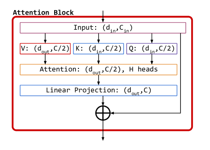
Figure 7: Attention block for the QM9 dataset. Each component is listed with a tuple of numbers representing the output feature types and multiplicities, so $(4,32)$ means feature types $0,1,2,3$ (with dimensionalities $1,3,5,7$), with 32 channels per type.

D.4 General Remark

Across experiments on different datasets with the SE(3)-Transformer, we made the observation that the number of representation degrees have a significant but saturating impact on performance. A big improvement was observed when switching from degrees $\{0,1\}$ to $\{0,1,2\}$. Adding type-3 latent representations gave small improvements, further representation degrees did not change the performance of the model. However, higher representation degrees have a significant impact on memory usage and computation time. We therefore recommend representation degrees up to 2, when computation time and memory usage is a concern, and 3 otherwise.

References

- Anderson et al. [2019] Brandon Anderson, Truong Son Hy, and Risi Kondor. Cormorant: Covariant molecular neural networks. In Advances in Neural Information Processing Systems (NeurIPS). 2019.
- Ba et al. [2016] Lei Jimmy Ba, Jamie Ryan Kiros, and Geoffrey E. Hinton. Layer normalization. arXiv Preprint, 2016.
- Ben-Shabat et al. [2018] Yizhak Ben-Shabat, Michael Lindenbaum, and Anath Fischer. 3dmfv: Three-dimensional point cloud classification in realtime using convolutional neural networks. IEEE Robotics and Automation Letters, 2018.
- Chen et al. [2019] Chao Chen, Guanbin Li, Ruijia Xu, Tianshui Chen, Meng Wang, and Liang Lin. ClusterNet: Deep Hierarchical Cluster Network with Rigorously Rotation-Invariant Representation for Point Cloud Analysis. In Proceedings of the IEEE Conference on Computer Vision and Pattern Recognition (CVPR), 2019.
- Chirikjian et al. [2001] Gregory S Chirikjian, Alexander B Kyatkin, and AC Buckingham. Engineering applications of noncommutative harmonic analysis: with emphasis on rotation and motion groups. Appl. Mech. Rev., 54(6):B97–B98, 2001.
- Cohen and Welling [2017] Taco S. Cohen and Max Welling. Steerable cnns. International Conference on Learning Representations (ICLR), 2017.
- Cohen et al. [2018] Taco S. Cohen, Mario Geiger, Jonas Koehler, and Max Welling. Spherical cnns. In International Conference on Learning Representations (ICLR), 2018.
- Finzi et al. [2020] Marc Finzi, Samuel Stanton, Pavel Izmailov, and Andrew Wilson. Generalizing convolutional neural networks for equivariance to lie groups on arbitrary continuous data. Proceedings of the International Conference on Machine Learning, ICML, 2020.
- Fuchs et al. [2020] Fabian B. Fuchs, Adam R. Kosiorek, Li Sun, Oiwi Parker Jones, and Ingmar Posner. End-to-end recurrent multi-object tracking and prediction with relational reasoning. arXiv preprint, 2020.
- Gilmer et al. [2020] Justin Gilmer, Samuel S. Schoenholz, Patrick F. Riley, and Oriol Vinyals George E. Dahl. Neural message passing for quantum chemistry. Proceedings of the International Conference on Machine Learning, ICML, 2020.
- Hirn et al. [2017] Matthew J. Hirn, Stéphane Mallat, and Nicolas Poilvert. Wavelet scattering regression of quantum chemical energies. Multiscale Model. Simul., 15(2):827–863, 2017.
- Hoshen [2017] Yedid Hoshen. Vain: Attentional multi-agent predictive modeling. Advances in Neural Information Processing Systems (NeurIPS), 2017.
- Kingma and Ba [2015] Diederik P. Kingma and Jimmy Ba. Adam: A method for stochastic optimization. In International Conference on Learning Representations, ICLR, 2015.
- Kipf et al. [2018] Thomas N. Kipf, Ethan Fetaya, Kuan-Chieh Wang, Max Welling, and Richard S. Zemel. Neural relational inference for interacting systems. In Proceedings of the International Conference on Machine Learning, ICML, 2018.
- Kondor [2018] Risi Kondor. N-body networks: a covariant hierarchical neural network architecture for learning atomic potentials. arXiv preprint, 2018.
- Lee et al. [2019] Juho Lee, Yoonho Lee, Jungtaek Kim, Adam R. Kosiorek, Seungjin Choi, and Yee Whye Teh. Set transformer: A framework for attention-based permutation-invariant neural networks. In Proceedings of the International Conference on Machine Learning, ICML, 2019.
- Lin et al. [2017] Zhouhan Lin, Minwei Feng, Cicero Nogueira dos Santos, Mo Yu, Bing Xiang, Bowen Zhou, and Yoshua Bengio. A structured self-attentive sentence embedding. International Conference on Learning Representations (ICLR), 2017.
- Parmar et al. [2019] Niki Parmar, Prajit Ramachandran, Ashish Vaswani, Irwan Bello, Anselm Levskaya, and Jon Shlens. Stand-alone self-attention in vision models. In Advances in Neural Information Processing System (NeurIPS), 2019.
- Qi et al. [2017a] Charles R Qi, Hao Su, Kaichun Mo, and Leonidas J Guibas. Pointnet: Deep learning on point sets for 3d classification and segmentation. IEEE Conference on Computer Vision and Pattern Recognition (CVPR), 2017a.
- Qi et al. [2017b] Charles R Qi, Li Yi, Hao Su, and Leonidas J Guibas. Pointnet++: Deep hierarchical feature learning on point sets in a metric space. Advances in Neural Information Processing Systems (NeurIPS), 2017b.
- Ramakrishnan et al. [2014] Raghunathan Ramakrishnan, Pavlo Dral, Matthias Rupp, and Anatole von Lilienfeld. Quantum chemistry structures and properties of 134 kilo molecules. Scientific Data, 1, 08 2014.
- Rao et al. [2019] Yongming Rao, Jiwen Lu, and Jie Zhou. Spherical fractal convolutional neural networks for point cloud recognition. In Proceedings of the IEEE Conference on Computer Vision and Pattern Recognition (CVPR), 2019.
- Rao et al. [2020] Yongming Rao, Jiwen Lu, and Jie Zhou. Global-local bidirectional reasoning for unsupervised representation learning of 3d point clouds. In Proceedings of the IEEE Conference on Computer Vision and Pattern Recognition (CVPR), 2020.
- Romero et al. [2020] David W. Romero, Erik J. Bekkers, Jakub M. Tomczak, and Mark Hoogendoorn. Attentive group equivariant convolutional networks. Proceedings of the International Conference on Machine Learning (ICML), 2020.
- Schütt et al. [2017] K. T. Schütt, P.-J. Kindermans, H. E. Sauceda, S. Chmiela1, A. Tkatchenko, and K.-R. Müller. Schnet: A continuous-filter convolutional neural network for modeling quantum interactions. Advances in Neural Information Processing Systems (NeurIPS), 2017.
- Shaw et al. [2018] Peter Shaw, Jakob Uszkoreit, and Ashish Vaswani. Self-attention with relative position representations. Annual Conference of the North American Chapter of the Association for Computational Linguistics (NAACL-HLT), 2018.
- Sosnovik et al. [2020] Ivan Sosnovik, Michał Szmaja, and Arnold Smeulders. Scale-equivariant steerable networks. International Conference on Learning Representations (ICLR), 2020.
- Thomas et al. [2018] Nathaniel Thomas, Tess Smidt, Steven M. Kearnes, Lusann Yang, Li Li, Kai Kohlhoff, and Patrick Riley. Tensor field networks: Rotation- and translation-equivariant neural networks for 3d point clouds. ArXiv Preprint, 2018.
- Uy et al. [2019] Mikaela Angelina Uy, Quang-Hieu Pham, Binh-Son Hua, Duc Thanh Nguyen, and Sai-Kit Yeung. Revisiting point cloud classification: A new benchmark dataset and classification model on real-world data. In International Conference on Computer Vision (ICCV), 2019.
- van Steenkiste et al. [2018] Sjoerd van Steenkiste, Michael Chang, Klaus Greff, and Jürgen Schmidhuber. Relational neural expectation maximization: Unsupervised discovery of objects and their interactions. International Conference on Learning Representations (ICLR), 2018.
- Vaswani et al. [2017] Ashish Vaswani, Noam Shazeer, Niki Parmar, Jakob Uszkoreit, Llion Jones, Aidan N. Gomez, Lukasz Kaiser, and Illia Polosukhin. Attention is all you need. Advances in Neural Information Processing Systems (NeurIPS), 2017.
- Veličković et al. [2018] Petar Veličković, Guillem Cucurull, Arantxa Casanova, Adriana Romero, Pietro Liò, and Yoshua Bengio. Graph attention networks. International Conference on Learning Representations (ICLR), 2018.
- Wagstaff et al. [2019] Edward Wagstaff, Fabian B. Fuchs, Martin Engelcke, Ingmar Posner, and Michael A. Osborne. On the limitations of representing functions on sets. International Conference on Machine Learning (ICML), 2019.
- Wang et al. [2017] Xiaolong Wang, Ross Girshick, Abhinav Gupta, and Kaiming He. Non-local neural networks. IEEE Conference on Computer Vision and Pattern Recognition (CVPR), 2017.
- Wang et al. [2019] Yue Wang, Yongbin Sun, Ziwei Liu, Sanjay E. Sarma, Michael M. Bronstein, and Justin M. Solomon. Dynamic graph cnn for learning on point clouds. ACM Transactions on Graphics (TOG), 2019.
- Weiler and Cesa [2019] Maurice Weiler and Gabriele Cesa. General E(2)-Equivariant Steerable CNNs. In Conference on Neural Information Processing Systems (NeurIPS), 2019.
- Weiler et al. [2018] Maurice Weiler, Mario Geiger, Max Welling, Wouter Boomsma, and Taco Cohen. 3d steerable cnns: Learning rotationally equivariant features in volumetric data. In Advances in Neural Information Processing Systems (NeurIPS), 2018.
- Winkels and Cohen [2018] Marysia Winkels and Taco S. Cohen. 3d g-cnns for pulmonary nodule detection. 1st Conference on Medical Imaging with Deep Learning (MIDL), 2018.
- Worrall and Welling [2019] Daniel E. Worrall and Max Welling. Deep scale-spaces: Equivariance over scale. In Advances in Neural Information Processing Systems (NeurIPS), 2019.
- Worrall et al. [2017] Daniel E. Worrall, Stephan J. Garbin, Daniyar Turmukhambetov, and Gabriel J. Brostow. Harmonic networks: Deep translation and rotation equivariance. IEEE Conference on Computer Vision and Pattern Recognition (CVPR), 2017.
- Wu et al. [2015] Zhirong Wu, Shuran Song, Aditya Khosla, Fisher Yu, Linguang Zhang, Xiaoou Tang, and Jianxiong Xiao. 3d shapenets: A deep representation for volumetric shapes. IEEE Conference on Computer Vision and Pattern Recognition (CVPR), 2015.
- Xie et al. [2018] Saining Xie, Sainan Liu, and Zeyu Chen Zhuowen Tu. Attentional shapecontextnet for point cloud recognition. IEEE Conference on Computer Vision and Pattern Recognition (CVPR), 2018.
- Xu et al. [2018] Yifan Xu, Tianqi Fan, Mingye Xu, Long Zeng, and Yu Qiao. Spidercnn: Deep learning on point sets with parameterized convolutional filters. European Conference on Computer Vision (ECCV), 2018.
- Yang et al. [2019] Jiancheng Yang, Qiang Zhang, and Bingbing Ni. Modeling point clouds with self-attention and gumbel subset sampling. IEEE Conference on Computer Vision and Pattern Recognition (CVPR), 2019.
- You et al. [2019] Yang You, Yujing Lou, Qi Liu, Yu-Wing Tai, Lizhuang Ma, Cewu Lu, and Weiming Wang. Pointwise Rotation-Invariant Network with Adaptive Sampling and 3D Spherical Voxel Convolution. In AAAI Conference on Artificial Intelligence, 2019.
- Zaheer et al. [2017] Manzil Zaheer, Satwik Kottur, Siamak Ravanbhakhsh, Barnabás Póczos, Ruslan Salakhutdinov, and Alexander Smola. Deep Sets. In Advances in Neural Information Processing Systems (NeurIPS), 2017.
- Zhang et al. [2019] Zhiyuan Zhang, Binh-Son Hua, David W. Rosen, and Sai-Kit Yeung. Rotation invariant convolutions for 3d point clouds deep learning. In International Conference on 3D Vision (3DV), 2019.