Parameterized Inapproximability
of Independent Set in $H$-Free Graphs

Abstract

We study the Independent Set problem in $H$-free graphs, i.e., graphs excluding some fixed graph $H$ as an induced subgraph. We prove several inapproximability results both for polynomial-time and parameterized algorithms.

Halldórsson [SODA 1995] showed that for every $\delta>0$ the Independent Set problem has a polynomial-time $(\frac{d-1}{2}+\delta)$-approximation algorithm in $K_{1,d}$-free graphs. We extend this result by showing that $K_{a,b}$-free graphs admit a polynomial-time $\mathcal{O}(\alpha(G)^{1-1/a})$-approximation, where $\alpha(G)$ is the size of a maximum independent set in $G$. Furthermore, we complement the result of Halldórsson by showing that for some $\gamma=\Theta(d/\log d),$ there is no polynomial-time $\gamma$-approximation algorithm for these graphs, unless NP = ZPP.

Bonnet et al. [Algorithmica 2020] showed that Independent Set parameterized by the size $k$ of the independent set is W[1]-hard on graphs which do not contain (1) a cycle of constant length at least $4$, (2) the star $K_{1,4}$, and (3) any tree with two vertices of degree at least $3$ at constant distance. We strengthen this result by proving three inapproximability results under different complexity assumptions for almost the same class of graphs (we weaken conditions (1) and (2) that $G$ does not contain a cycle of constant length at least 5 or $K_{1,5}$). First, under the ETH, there is no $f(k)\cdot n^{o(k/\log k)}$ algorithm for any computable function $f$. Then, under the deterministic Gap-ETH, there is a constant $\delta>0$ such that no $\delta$-approximation can be computed in $f(k)\cdot n^{O(1)}$ time. Also, under the stronger randomized Gap-ETH there is no such approximation algorithm with runtime $f(k)\cdot n^{o(\sqrt{k})}$.

Finally, we consider the parameterization by the excluded graph $H$, and show that under the ETH, Independent Set has no $n^{o(\alpha(H))}$ algorithm in $H$-free graphs. Also, we prove that there is no $d/k^{o(1)}$-approximation algorithm for $K_{1,d}$-free graphs with runtime $f(d,k)\cdot n^{\mathcal{O}(1)}$, under the deterministic Gap-ETH.

1 Introduction

The Independent Set problem, which asks for a maximum sized set of pairwise non-adjacent vertices in a graph, is one of the most well-studied problems in algorithmic graph theory. It was among the first 21 problems that were proven to be NP-hard by Karp [30], and is also known to be hopelessly difficult to approximate in polynomial time: Håstad [29] proved that under standard assumptions from classical complexity theory the problem admits no $(n^{1-\varepsilon})$-approximation, for any $\varepsilon>0$ (by $n$ we always denote the number of vertices in the input graph). This was later strengthened by Khot and Ponnuswami [31], who were able to exclude any algorithm with approximation ratio $n/(\log n)^{3/4+\varepsilon}$, for any $\varepsilon>0$. Let us point out that the currently best polynomial-time approximation algorithm for Independent Set achieves the approximation ratio $\mathcal{O}(n\frac{(\log\log n)^{2}}{(\log n)^{3}})$ [21].

There are many possible ways of approaching such a difficult problem, in order to obtain some positive results. One could give up on generality, and ask for the complexity of the problem on restricted instances. For example, while the Independent Set problem remains NP-hard in subcubic graphs [24], a straightforward greedy algorithm gives a 3-approximation.

$H$-free graphs.

A large family of restricted instances, for which the Independent Set problem has been well-studied, comes from forbidding certain induced subgraphs. For a (possibly infinite) family $\mathcal{H}$ of graphs, a graph $G$ is $\mathcal{H}$-free if it does not contain any graph of $\mathcal{H}$ as an induced subgraph. If $\mathcal{H}$ consists of just one graph, say $\mathcal{H}=\{H\}$, then we say that $G$ is $H$-free. The investigation of the complexity of Independent Set in $\mathcal{H}$-free graphs dates back to Alekseev, who observed that the so-called “Poljak construction” [44] yields the following.

Theorem 1.1 (Alekseev [2], Poljak [44]).

Let $s\geq 3$ be a constant. The Independent Set problem is NP-hard in graphs that do not contain any of the following induced subgraphs:

1. a cycle on at most $s$ vertices,

2. the star $K_{1,4}$, and

3. any tree with two vertices of degree at least 3 at distance at most $s$.

We can restate Theorem 1.1 as follows: the Independent Set problem is NP-hard in $H$-free graphs, unless $H$ is a subgraph of a subdivided claw (i.e., three paths which meet at one of their endpoints). The reduction also implies that for each such $H$ the problem is APX-hard and cannot be solved in subexponential time, unless the Exponential Time Hypothesis (ETH) fails. On the other hand, polynomial-time algorithms are known only for very few cases. First let us consider the case when $H=P_{t}$, i.e., we forbid a path on $t$ vertices. Note that the case of $t=3$ is trivial, as every $P_{3}$-free graph is a disjoint union of cliques. Already in 1981 Corneil, Lerchs, and Burlingham [14] showed that Independent Set is tractable for $P_{4}$-free graphs. For many years there was no improvement, until the breakthrough algorithm of Lokshtanov, Vatshelle, and Villanger [34] for $P_{5}$-free graphs. Their approach later recently extended to $P_{6}$-free graphs by Grzesik, Klimošova, Pilipczuk, and Pilipczuk [27]. The general belief that the problem should be polynomial-time solvable for $P_{t}$-free graphs, for any fixed $t$, is suppotred by recent quasipolynomial-time algorithm by Gartland and Lokshtanov [25]; see also a simplified version of Pilipczuk, Pilipczuk, and Rzążewski [43].

Even less is known for the case if $H$ is a subdivided claw. The problem can be solved in polynomial time in claw-free (i.e., $K_{1,3}$-free) graphs, see Sbihi [45] and Minty [42]. This was later extended to $H$-free graphs, where $H$ is a claw with one edge once subdivided (see Alekseev [1] for the unweighted version and Lozin, Milanič [36] for the weighted one). We also know that for any subdivided claw $H$, the problem can be solved in subexponential time in $H$-free graphs [13, 37].

When it comes to approximations, Halldórsson [28] gave an elegant local search algorithm that finds a $(\frac{d-1}{2}+\delta)$-approximation of a maximum independent set in $K_{1,d}$-free graphs for any constant $\delta>0$ in polynomial time. Chudnovsky, Thomassé, Pilipczuk, and Pilipczuk [13] designed a QPTAS (quasi-polynomial-time approximation scheme) that works for subdivided claw $H$; see also the improved version of Majewski et al. [37]. Recall that if $H$ is not (a subgraph of) a subdivided claw, then the problem is APX-hard. The existence of algorithms for MIS in $H$-free graph with approximation guararantee $n^{1-\delta}$ for constant $\delta$ was studied recently by Bonnet et al. [8] in the connection to the famous Erdős-Hajnal conjecture.

Parameterized complexity.

Another approach that one could take is to look at the problem from the parameterized perspective: we no longer insist on finding a maximum independent set, but want to verify whether some independent set of size at least $k$ exists. To be more precise, we are interested in knowing how the complexity of the problem depends on $k$. The best type of behavior we are hoping for is fixed-parameter tractability (FPT), i.e., the existence of an algorithm with running time $f(k)\cdot n^{\mathcal{O}(1)}$, for some function $f$ (note that since the problem is NP-hard, we expect $f$ to be super-polynomial).

It is known [15] that on general graphs the Independent Set problem is W[1]-hard parameterized by $k$, which is a strong indication that it does not admit an FPT algorithm. Furthermore, it is even unlikely to admit any non-trivial fixed-parameter approximation (FPA): a $\beta$-FPA algorithm (for $\beta>1$) for the Independent Set problem is an algorithm that takes as input a graph $G$ and an integer $k$, and in time $f(k)\cdot n^{\mathcal{O}(1)}$ either correctly concludes that $G$ has no independent set of size at least $k$, or outputs an independent set of size at least $k/\beta$ (note that $\beta$ does not have to be a constant). It was shown in [9] that on general graphs no $o(k)$-FPA exists for Independent Set, unless the deterministic Gap-ETH fails.

Parameterized complexity in $H$-free graphs.

As we pointed out, none of the discussed approaches, i.e., considering $H$-free graphs or considering parameterized algorithms, seems to make the Independent Set problem more tractable. However, some positive results can be obtained by combining these two settings, i.e., considering the parameterized complexity of Independent Set in $H$-free graphs. For example, the Ramsey theorem implies that any graph with $\Omega(4^{p})$ vertices contains a clique or an independent set of size $\Omega(p)$. Since the proof actually tells us how to construct a clique or an independent set in polynomial time [20], we immediately obtain a very simple FPT algorithm for $K_{p}$-free graphs. Dabrowski [16] provided some positive and negative results for the complexity of the Independent Set problem in $H$-free graphs, for various $H$. The systematic study of the problem was initiated by Bonnet, Bousquet, Charbit, Thomassé, and Watrigant [6] and continued by Bonnet, Bousquet, Thomassé, and Watrigant [7]. Among other results, Bonnet et al. [6] obtained the following analog of Theorem 1.1.

Theorem 1.2 (Bonnet et al. [6]).

Let $s\geq 4$ be a constant. The Independent Set problem is W[1]-hard in graphs that do not contain any of the following induced subgraphs:

1. a cycle on at least 4 and at most $s$ vertices,

2. the star $K_{1,4}$, and

3. any tree with two vertices of degree at least 3 at distance at most $s$.

Note that, unlike in Theorem 1.1, we are not able to show hardness for $C_{3}$-free graphs: as already mentioned, the Ramsey theorem implies that Independent Set is FPT in $C_{3}$-free graphs. Thus, graphs $H$ for which there is hope for FPT algorithms in $H$-free graphs are essentially obtained from paths and subdivided claws (or their subgraphs) by replacing each vertex with a clique.

Let us point out that, even though it is not stated there explicitly, the reduction of Bonnet et al. [6] also excludes any algorithm solving the problem in time $f(k)\cdot n^{o(\sqrt{k})}$, unless the ETH fails.

Our results.

We study the approximation of the Independent Set problem in $H$-free graphs, mostly focusing on approximation hardness. Our first two results are related to Halldórsson’s [28] polynomial-time $(\frac{d-1}{2}+\delta)$-approximation algorithm for $K_{1,d}$-free graphs. First, in Section 3 we extend this result to $K_{a,b}$-free graphs, for any constants $a,b$, showing the following theorem.

Theorem 1.3 ().

Given a $K_{a,b}$-free graph $G$, an $\mathcal{O}\bigl{(}(a+b)^{1/a}\cdot\alpha(G)^{1-1/a}\bigr{)}$-approximation can be computed in $n^{\mathcal{O}(a)}$ time.

Then, in Section 4 we show that the approximation ratio of the algorithm of Halldórsson [28] is optimal, up to logarithmic factors.

Theorem 1.4 ().

There is a constant $d^{\star}$ and a function $\beta=\Theta(d/\log d)$ such that for any $d\geq d^{\star}$ the Independent Set problem does not admit a polynomial time $\beta$-approximation algorithm in $K_{1,d}$-free graphs, unless ZPP = NP.

We remark that for graphs of maximum degree $d$, which are also $K_{1,d}$-free, Independent Set admits a polynomial time $\tilde{O}(d/\log^{2}d)$-approximation [4] (where the $\tilde{O}$-notation hides poly($\log\log d$) factors) and this is tight [3] (up to poly($\log\log d$) factors) under the Unique Games Conjecture. Also, assuming P $\neq$ NP no $\mathcal{O}(d/\log^{4}d)$-approximation exists [10]. This means that the hardness of Theorem 1.4 together with the algorithm in [4] give a separation between graphs of maximum degree $d$ and $K_{1,d}$-free graphs in terms of approximation.

Then in Section 5 we study the existence of fixed-parameter approximation algorithms (cf. [23]) for the Independent Set problem in $H$-free graphs. We show the following strengthening of Theorem 1.2, which also gives (almost) tight runtime lower bounds assuming the ETH or the randomized Gap-ETH (for more information about complexity assumptions used in the following theorems see Section 2).

Theorem 1.5 ().

Let $s\geq 5$ be a constant, and let $\mathcal{G}$ be the class of graphs that do not contain any of the following induced subgraphs:

1. a cycle on at least 5 and at most $s$ vertices,

2. the star $K_{1,5}$, and

3. 1. the star $K_{1,4}$, or

   2. a cycle on 4 vertices and any tree with two vertices of degree at least 3 at distance at most $s$.

The Independent Set problem on $\mathcal{G}$ does not admit the following:

1. an exact algorithm with runtime $f(k)\cdot n^{o(k/\log k)}$, for any computable function $f$, under the ETH,

2. a $\beta$-approximation algorithm with runtime $f(k)\cdot n^{\mathcal{O}(1)}$ for some constant $\beta>1$ and any computable function $f$, under the deterministic Gap-ETH,

3. a $\beta$-approximation algorithm with runtime $f(k)\cdot n^{o(\sqrt{k})}$ for some constant $\beta>1$ and any computable function $f$, under the randomized Gap-ETH.

By gap amplification using the lexicographical graph product, we are able to strengthen statement (b) of Theorem 1.5, but we need to consider a larger class of graphs to obtain the lower bound. We say two vertices $u,v$ are twins if, apart from the adjacency between them, their neighborhoods are the same, i.e., $N(u)\setminus\{v\}=N(v)\setminus\{u\}$.

Theorem 1.6 ().

Let $s\geq 5$ be a constant, and let $\mathcal{G}^{\prime}$ be the class of graphs that do not contain any of the following induced subgraphs:

1. a cycle on at least 5 and at most $s$ vertices, and

2. any tree without twins and with two vertices of degree at least 3 at distance at most $s$.

Then for any constant $\beta>1$, the Independent Set problem on $\mathcal{G}^{\prime}$ does not admit a $\beta$-approximation algorithm with runtime $f(k)\cdot n^{\mathcal{O}(1)}$ for any computable function $f$, under the deterministic Gap-ETH.

In contrast with statement (b) of Theorem 1.5, Theorem 1.6 refuses any constant-factor FPT approximation for the Independent Set problem on the class $\mathcal{G}^{\prime}$. However, the gap amplification works only for forbidden graphs without twins. Thus, the class $\mathcal{G}^{\prime}$ is larger than the class $\mathcal{G}$ defined in Theorem 1.5, and the family of forbidden subgraphs of $\mathcal{G}^{\prime}$ is exactly the family of forbidden subgraphs of $\mathcal{G}$ restricted to graphs without twins. We prove Theorem 1.6 in Section 5.3.

Finally, in Section 6 we study a slightly different setting, where the graph $H$ is not considered to be fixed. As mentioned before, Independent Set is known to be polynomial-time solvable in $P_{t}$-free graphs for $t\leq 6$. The algorithms for increasing values of $t$ get significantly more complicated and their complexity increases. Thus it is natural to ask whether this is an inherent property of the problem and can be formalized by a runtime lower bound when parameterized by $t$.

We give an affirmative answer to this question, even if the forbidden family is not a family of paths: note that the independent set number $\alpha(P_{t})$ of a path on $t$ vertices is $\lceil t/2\rceil$.

Proposition 1 ().

For any integer $d$, let $\mathcal{H}_{d}$ be a class of graphs so that $\alpha(H)>d$ for every $H\in\mathcal{H}_{d}$, and let $\zeta$ be any function in $\omega(1)$. Consider an instance $(G,k)$ of Independent Set and let $d$ be the minimum value for which $G$ is $\mathcal{H}_{d}$-free. The Independent Set problem is W[1]-hard parameterized by $d$ and cannot be solved in $n^{o(d)}$ time, unless the ETH fails. Furthermore, no $d^{o(1)}$-approximation can be computed in $f(d)n^{\mathcal{O}(1)}$ time under ETH, and no independent set of size $\zeta(d)$ can be computed in $f(d)n^{\zeta(d)}$ time under the deterministic Gap-ETH.

We also study the special case when $H=K_{1,d}$ and consider the inapproximability of the problem parameterized by both $\alpha(K_{1,d})=d$ and $k$. Unfortunately, for the parameterized version we do not obtain a clear-cut statement as in Theorem 1.4, since in the following theorem $d$ cannot be chosen independently of $k$ in order to obtain an inapproximability gap.

Proposition 2 ().

Let $\varepsilon>0$ be any constant, $\xi(k)=2^{(\log k)^{1/2+\varepsilon}}$, and $\zeta$ be any function in $\omega(1)$. The Independent Set problem in $K_{1,d}$-free graphs has no $d/\xi(k)$- and no $d/\zeta(k)$-approximation algorithm with runtime $f(d,k)\cdot n^{\mathcal{O}(1)}$ for any computable function $f$, unless the deterministic Gap-ETH or the Strongish Planted Clique Hypothesis fails, respectively.

Note that this in particular shows that if we allow $d$ to grow as a polynomial $k^{\varepsilon}$ for any constant $0<\varepsilon<1/2$, then no $k^{\delta}$-approximation is possible for any $\delta<\varepsilon$ (since $\xi(k)=k^{o(1)}$), under the deterministic Gap-ETH. Under the Strongish Planted Clique Hypothesis, we can even allow $d$ to grow arbitrarily slowly in $k$ and still get an approximation lower bound. This indicates that the $(\frac{d-1}{2}+\delta)$-approximation for $K_{1,d}$-free graphs [28] is likely to be best possible (up to sub-polynomial factors), even when parameterizing by $k$ and $d$. The proofs of Proposition 1 and Proposition 2 can be found in Section 6.

2 Preliminaries

All our hardness results for Independent Set are obtained by reductions from some variant of the Maximum Colored Subgraph Isomorphism (MCSI) problem. This optimization problem has been widely studied in the literature, both to obtain polynomial-time and parameterized inapproximability results, but also in its decision version to obtain parameterized runtime lower bounds. We note that by applying standard transformations, MCSI contains the well-known problems Label Cover [32] and Binary CSP [35]: for Binary CSP the graph $J$ is a complete graph, while for Label Cover $J$ is usually bipartite.

Maximum Colored Subgraph Isomorphism (MCSI)
Input:	A graph $G$, whose vertex set is partitioned into subsets $V_{1},\dots,V_{\ell}$, and a graph $J$ on vertex set $\{1,\dots,\ell\}$.
Goal:	Find an assignment $\phi:V(J)\to V(G)$, where $\phi(i)\in V_{i}$ for every $i\in[\ell]$, that maximizes the number $S(\phi)$ of satisfied edges, i.e., $S(\phi):=\bigl{|}\bigl{\{}ij\in E(J)\;|\;\phi(i)\phi(j)\in E(G)\bigr{\}}\bigr{|}.$

Given an instance $\Gamma=(G,V_{1},\ldots,V_{\ell},J)$ of MCSI, we refer to the number of vertices of $G$ as the size of $\Gamma$. Any assignment $\phi:V(J)\to V(G)$, such that for every $i$ it holds that $\phi(i)\in V_{i}$, is called a solution of $\Gamma$. The value of a solution $\phi$ is $\operatorname{val}(\phi):=S(\phi)/|E(J)|$, i.e., the fraction of satisfied edges. The value of the instance $\Gamma$, denoted by $\operatorname{val}(\Gamma)$, is the maximum value of any solution of $\Gamma$.

When considering the decision version of MCSI, i.e., determining whether $\operatorname{val}(\Gamma)=1$ or $\operatorname{val}(\Gamma)<1$, a classic hardness result for Multicolored Clique (i.e., if $J$ is a complete graph) implies that that under the Exponential Time Hypothesis (ETH) the problem cannot be solved in $f(\ell)\cdot n^{o(\ell)}$ time for any computable function $f$. For the optimization version of MCSI, an $\alpha$-approximation is a solution $\phi$ with $\operatorname{val}(\phi)\geq 1/\alpha$. When $J$ is a complete graph, a result by Dinur and Manurangsi [17, 18] states that there is no $\ell/\xi(\ell)$-approximation algorithm, where $\xi(\ell)=2^{(\log\ell)^{1/2+\varepsilon}}=\ell^{o(1)}$ for any constant $\varepsilon>0$, with runtime $f(\ell)\cdot n^{O(1)}$ for any computable function $f$, unless the deterministic Gap-ETH fails (see Theorem 6.3). This hypothesis assumes that there exists some constant $\delta>0$ such that no deterministic $2^{o(n)}$ time algorithm for 3-SAT can decide whether all or at most a $(1-\delta)$-fraction of the clauses can be satisfied. A recent result by Manurangsi [38] uses an even stronger assumption, which also rules out randomized algorithms, and in turn obtains a better runtime lower bound at the expense of a worse approximation lower bound: when $J$ is a complete graph, there is no $\beta$-approximation algorithm for MCSI with runtime $f(\ell)\cdot n^{o(\ell)}$ for any computable function $f$ and any constant $\beta$, under the randomized Gap-ETH. This assumes that there exists some constant $\delta>0$ such that no randomized $2^{o(n)}$ time algorithm for 3-SAT can decide whether all or at most a $(1-\delta)$-fraction of the clauses can be satisfied. Another related conjecture that was recently used to obtain lower bounds for MCSI where $J$ is a clique, is the Strongish Planted Clique Hypothesis. It states that no randomized algorithm with runtime $n^{o(\log n)}$ can find a planted clique of size $n^{\delta}$ for some $0<\delta<1/2$ in a random graph on $n$ vertices. Manurangsi et al. [39] prove that under this conjecture, no $f(\ell)\cdot n^{O(1)}$ time algorithm can compute a $o(\ell)$-approximation to MCSI (see Theorem 6.3).

For our results we will often need the special case of MCSI when the graph $J$ has bounded degree. We define this problem in the following.

Degree-$t$ Maximum Colored Subgraph Isomorphism (MCSI($t$))
Input:	A graph $G$, whose vertex set is partitioned into subsets $V_{1},\dots,V_{\ell}$, and a graph $J$ on vertex set $\{1,\dots,\ell\}$ and maximum degree $t$.
Goal:	Find an assignment $\phi:V(J)\to V(G)$, where $\phi(i)\in V_{i}$ for every $i\in[\ell]$, that maximizes the number $S(\phi)$ of satisfied edges, i.e., $S(\phi):=\bigl{|}\bigl{\{}ij\in E(J)\;|\;\phi(i)\phi(j)\in E(G)\bigr{\}}\bigr{|}.$

The bounded degree case has been considered before, and we harness some of the known hardness results for MCSI($t$) in our proofs. First, a reduction of Marx [40] implies that assuming the ETH, MCSI($3$) cannot be solved in time $f(\ell)\cdot n^{o(\ell/\log\ell)}$, for any computable function $f$ (see also Marx and Pilipczuk [41, Theorem 5.5]). We also use a polynomial-time approximation lower bound given by Laekhanukit [32], where $t$ can be set to any constant and the approximation gap depends on $t$ (see Theorem 4.1). The complexity assumption of this reduction is that NP-hard problems do not have polynomial time Las Vegas algorithms, i.e., NP $\neq$ ZPP. For parameterized approximations, we use a result by Lokshtanov et al. [35], who obtain a constant approximation gap for the case when $t=3$ (see Theorem 5.2). It seems that this result for parameterized algorithms is not easily generalizable to arbitrary constants $t$ so that the approximation gap would depend only on $t$, as in the result for polynomial-time algorithms provided by Laekhanukit [32]: neither the techniques found in [32] nor those of [35] seem to be usable to obtain an approximation gap that depends only on $t$ but not the parameter $\ell$. However, we develop a weaker parameterized inapproximability result for the case when $t\geq\xi(\ell)=\ell^{o(1)}$ or $t\geq\zeta(\ell)=\omega(1)$ (see Theorem 6.1 in Section 6), and use it to prove Proposition 2.

3 Approximation for $K_{a,b}$-free Graphs

In this section we give a polynomial-time $\mathcal{O}\bigl{(}(a+b)^{1/a}\cdot\alpha(G)^{1-1/a}\bigr{)}$-approximation algorithm for Independent Set on $K_{a,b}$-free graphs, where $\alpha(G)$ is the size of a maximum independent set in the input graph $G$. The algorithm is a generalization of a known local search procedure. Note that it asymptotically matches the approximation factor of the $(\frac{d-1}{2}+\delta)$-approximation algorithm for $K_{1,d}$-free graphs of Halldórsson [28] by setting $a=1$ and $b=d$. We note here that the following theorem was independently discovered by Bonnet, Thomassé, Tran, and Watrigant [8].

See 1.3

Proof.

The algorithm first computes a maximal independent set $I\subseteq V(G)$ in the given graph $G$, which can be done in linear time using a simple greedy approach. Since $I$ is maximal, every vertex in $V(G)\setminus I$ has at least one neighbor in $I$. Now, we consider the vertices in $V(G)\setminus I$ that are neighbors to at most $a-1$ vertices of $I$, and call this set $V_{1}$. Let $C\subseteq I$ be a set of size $c\in[a-1]$, and let $V_{C}:=\{v\in V_{1}\mid N(v)\cap I=C\}$. If the graph induced by $V_{C}\cup C$ contains an independent set $I^{\prime}$ of size $|C|+1$, then we can find it in time $n^{\mathcal{O}(|C|+1)}=n^{\mathcal{O}(a)}$. Furthermore, $(I\setminus C)\cup I^{\prime}$ is an independent set, since no vertex of $V_{C}\cup C$ is adjacent to any vertex of $I\setminus C$, and $(I\setminus C)\cup I^{\prime}$ is larger by one than $I$. Thus the algorithm replaces $I\setminus C$ by $I^{\prime}$ in $I$. The algorithm repeats this procedure until the largest independent set in each subgraph induced by a set $V_{C}\cup C$ (defined for the current $I$) is of size at most $|C|$. At this point the algorithm outputs $I$.

Let $k=|I|$ be the size of the output at the end of the algorithm. We claim that $\alpha(G)\leq(a-1)k^{a-1}+(b-1)k^{a}=\mathcal{O}\bigl{(}(a+b)k^{a}\bigr{)}$ and this would prove the theorem, since then $k=\Omega\bigl{(}(\frac{\alpha(G)}{a+b})^{1/a}\bigr{)}$, which implies that $I$ is an $\mathcal{O}\bigl{(}(a+b)^{1/a}\cdot\alpha(G)^{1-1/a}\bigr{)}$-approximation.

To show the claim, first note that the family $\bigl{\{}V_{C}\ \mid C\subseteq I\text{ and }|C|\in[a-1]\bigr{\}}$ is a partition of $V_{1}$ into at most $\sum_{c=1}^{a-1}{k\choose c}$ many sets. For each relevant $C$, no subgraph induced by a set $V_{C}\cup C$ contains an independent set larger than $|C|$, and thus if $I^{*}$ denotes a maximum independent set of $G$, then $\bigl{|}(V_{C}\cup C)\cap I^{*}\bigr{|}\leq|C|$. Thus,

$$\bigl{|}(V_{1}\cup I)\cap I^{*}\bigr{|}\leq\sum_{c=1}^{a-1}c{k\choose c}=\sum_{c=1}^{a-1}k\binom{k-1}{c-1}\leq\sum_{c=1}^{a-1}k^{c}\leq(a-1)k^{a-1}.$$

Now consider the remaining set $V_{2}:=V(G)\setminus(V_{1}\cup I)$, and observe that every $v\in V_{2}$ has at least $a$ neighbors in $I$ due to the definition of $V_{1}$. For each $D\subseteq I$ with $|D|=a$, we construct a set $V_{D}$ by fixing an arbitrary subset $S(v)\subseteq(N(v)\cap I)$ of size $a$ for every $v\in V_{2}$, and putting $v$ into $V_{D}$ if and only if $S(v)=D$. Observe that these sets $V_{D}$ form a partition of $V_{2}$ of size at most ${k\choose a}$. We claim that each $V_{D}$ induces a subgraph of $G$ for which every independent set has size less than $b$. Assume not, and let $I^{\prime}$ be an independent set in $V_{D}$ of size $b$. But then $D\cup I^{\prime}$ induces a $K_{a,b}$ in $G$, since every vertex of $I^{\prime}\subseteq V_{D}$ is adjacent to every vertex of $D\subseteq I$. As this contradicts the fact that $G$ is $K_{a,b}$-free, we have $|V_{D}\cap I^{*}|\leq b-1$, and consequently $|V_{2}\cap I^{*}|\leq(b-1){k\choose a}\leq(b-1)k^{a}$. Together with the above bound on the number of vertices of $I^{*}$ in $V_{1}\cup I$ we get

$$\alpha(G)=|I^{*}|\leq(a-1)k^{a-1}+(b-1)k^{a},$$

which concludes the proof. ∎

4 Polynomial Time Inapproximability in $K_{1,d}$-free Graphs

In this section, we show polynomial time approximation lower bounds for Independent Set on $K_{1,d}$-free graphs.

See 1.4

For that, we reduce from the MCSI($t$) problem, and leverage the lower bound by Laekhanukit [32, Theorem $6$]. Let us point out that the original statement of the lower bound by Laekhanukit [32] is in terms of the Label Cover problem, but, as we already mentioned, this is a special case of MCSI.

Theorem 4.1 (Laekhanukit [32]).

Let $\Gamma=(G,V_{1},\dots,V_{\ell},J)$ be an instance of MCSI($t$) where $J$ is a bipartite graph. Assuming ZPP $\neq$ NP, there exist constants $t^{\star}$ and $c$ such that for any constant $\varepsilon>0$ and any $t\geq t^{\star}$, there is no polynomial time algorithm that can distinguish between the two cases:

1. (YES-case) $\operatorname{val}(\Gamma)\geq 1-\varepsilon$, and

2. (NO-case) $\operatorname{val}(\Gamma)\leq c\log(t)/t+\varepsilon$.

We use a standard reduction from MCSI to Independent Set, which can be seen as a variant of the so-called FGLSS-graph [22]. For instances of MCSI($t$) with bounded degree $t$ gives the following lemma.

Lemma 1 ().

Let $\Gamma=(G,V_{1},\dots,V_{\ell},J)$ be an instance of MCSI($t$). Given $\Gamma$, in polynomial time we can construct an instance $G^{\prime}$ of Independent Set  such that

1. $G^{\prime}$ does not have $K_{1,d}$ as an induced subgraph for any $d\geq 2t+2$,

2. if $\operatorname{val}(\Gamma)\geq\mu$ then $G^{\prime}$ has an independent set of size at least $\mu|E(J)|$, and

3. if $\operatorname{val}(\Gamma)\leq\nu$ then every independent set of $G^{\prime}$ has size at most $\nu|E(J)|$.

Proof.

We first describe the construction of $G^{\prime}$ given $\Gamma=(G,V_{1},\dots,V_{\ell},J)$, where we denote by $E_{ij}$ the edge set between $V_{i}$ and $V_{j}$ for each edge $ij\in E(J)$. The graph $G^{\prime}$ has a vertex $v_{e}$ for each edge $e$ of $G$, an edge between $v_{e}$ and $v_{f}$ if $e,f\in E_{ij}$ for some $ij\in E(J)$, and an edge between $v_{e}$ and $v_{f}$ if $e\in E_{ij}$ and $f\in E_{ij^{\prime}}$ and $e$ and $f$ do not share a vertex in $G$ for some three vertices $i,j,j^{\prime}\in[\ell]$ of $J$ such that $ij\in E(J)$ and $ij^{\prime}\in E(J)$. Note that the vertex set $V^{\prime}_{ij}=\{v_{e}\in V(G^{\prime})\mid e\in E_{ij}\}$ induces a clique in $G^{\prime}$. This finishes the construction of $G^{\prime}$. See Figure 1 for better understanding of the construction.

Figure 1: Example of the construction of the graph $G^{\prime}$ from $G$ for $J$ being a path on 3 vertices.

To see the first part of the lemma, for the sake of contradiction, let us suppose $G^{\prime}$ has a $K_{1,d}$ as an induced subgraph for $d\geq 2t+2$. We know that for any $e\in E(J)$ the vertices in $V^{\prime}_{e}$ form a clique in $G^{\prime}$, so the star $K_{1,d}$ can intersect with a fixed $V^{\prime}_{e}$ in at most two vertices of which one must be the center vertex of $K_{1,d}$ with degree $d$. As $K_{1,d}$ has $d+1$ vertices, this means there are (at least) $d$ distinct vertex sets $V^{\prime}_{e_{1}},V^{\prime}_{e_{2}},\ldots,V^{\prime}_{e_{d}}$ of $G$ that intersect the $K_{1,d}$ for some edges $e_{1},e_{2},\ldots,e_{d}\in E(J)$. Without loss of generality, let the center vertex of the $K_{1,d}$ come from $V^{\prime}_{e_{1}}$. Note that the $K_{1,d}$ has an edge between a vertex from $V^{\prime}_{e_{1}}$ and a vertex from $V^{\prime}_{e_{z}}$ for each $z\in\{2,\ldots,d\}$. Hence if $e_{1}=jj^{\prime}$, we have that either $j\in e_{z}$ or $j^{\prime}\in e_{z}$ for every $z\in[d]$ by the construction of $G^{\prime}$. This means that either $j$ or $j^{\prime}$ has at least $(d-1)/2$ neighbours in $J$. That is, the maximum degree of $J$ is at least $(d-1)/2$. As $d\geq 2t+2$, we obtain that the maximum degree of $J$ is more than $t$, which is a contradiction with the definition of MCSI($t$).

Now, to see the second claim of the lemma, first we need to show that if $\operatorname{val}(\Gamma)\geq\mu$, then $G^{\prime}$ has an independent set of size at least $\mu|E(J)|$. To see that, let $\phi:V(J)\rightarrow V(G)$ be a mapping that satisfies at least a $\mu$-fraction of the edges of $E(J)$. We claim that $S=\{v_{uw}\in V^{\prime}_{ij}\mid ij\in E(J),\phi(i)=u,\phi(j)=w\}$ is an independent set of size at least $\mu|E(J)|$ in $G^{\prime}$. Since $\phi$ satisfies at least $\mu$-fraction of edges, $S$ has size at least $\mu|E(J)|$. So all we need to show is that $S$ is indeed an independent set. Suppose it was not the case, i.e., there exist $v_{e},v_{f}\in S$ that are adjacent in $G^{\prime}$. By construction of $G^{\prime}$ there can be an edge between $v_{e}$ and $v_{f}$ only if $e\in E_{ij}$ and $f\in E_{ij^{\prime}}$ where possibly $j=j^{\prime}$. Note that $\phi(i)=u\in V_{i}$ is a common endpoint of both $e$ and $f$. If indeed $j=j^{\prime}$, then $\phi(j)=w\in V_{j}$ is also a common endpoint of both $e$ and $f$, so that $e=f$, i.e., $v_{e}$ and $v_{f}$ are not distinct. Hence it must be that $j\neq j^{\prime}$. But in this case, the construction of $G^{\prime}$ implies that $e$ and $f$ do not share a vertex, which contradicts the fact that they have $u$ as a common endpoint.

For the third part of the lemma, we prove the contrapositive: we claim that if $G^{\prime}$ has an independent set $S$ of size $k\geq\nu|E(J)|$, then there exists an assignment $\phi:V(J)\rightarrow V(G)$ satisfying at least $k$ edges in $\Gamma$. To see that, first observe that the set $S$ can contain at most one vertex from $V^{\prime}_{e}$ as any two vertices in $V^{\prime}_{e}$ are adjacent. Let $E_{S}:=\{e\in E(J)\mid S\cap V^{\prime}_{e}\neq\emptyset\}$, for which we then have $|E_{S}|=|S|$. We claim that all the edges in $E_{S}$ can be satisfied by an assignment $\phi$ defined as follows. For $ij\in E_{S}$, let $S\cap V^{\prime}_{ij}=\{v_{uw}\}$. Then we set $\phi(i)=u$ and $\phi(j)=w$. We need to show that the function $\phi$ is well-defined. Suppose some vertex $i\in V(J)$ gets mapped to more than one vertex of $V(G)$ by $\phi$. This must mean that there exist two edges in $G$ that contain one endpoint in $V_{i}$ and are in $E_{S}$. But this would mean that the two vertices in $S$ corresponding to these two edges in $E_{S}$ are adjacent due to the construction of $G^{\prime}$. This is a contradiction to $S$ being an independent set. Also, $\phi(i)\phi(j)\in E(G)$ for all $ij\in E_{S}$, since for each $v_{uw}$ we have $uw\in E(G)$, and we have set $\phi(i)=u$ and $\phi(j)=w$. This concludes the proof. ∎

Now we are ready to prove Theorem 1.4.

Proof of Theorem 1.4.

Assume there was a polynomial time algorithm $\mathcal{A}$ to approximate the Independent Set problem within a factor $\frac{1-\varepsilon}{c\log(t)/t+\varepsilon}$ for some $\varepsilon>0$ in $K_{1,d}$-free graphs, where $t=\lfloor\frac{d}{2}-1\rfloor\geq t^{\star}$, and $c$ is the constant given by Theorem 4.1. Given an instance $\Gamma=(G,V_{1},\dots,V_{\ell},J)$ of MCSI($t$) and $\varepsilon$, we can reduce it to an instance of Independent Set in $K_{1,d}$-free graphs in polynomial time by using the reduction of Lemma 1. Now, setting $\mu=1-\varepsilon$ and $\nu=(c\log(t)/t)+\varepsilon$ in the statement of Lemma 1, this gives that given an instance $\Gamma$ of MCSI($t$) and $\varepsilon$, we can now use $\mathcal{A}$ to differentiate between the YES- and NO-cases of Theorem 4.1 in polynomial time, which would mean that ZPP = NP. As $\frac{1-\varepsilon}{c\log(t)/t+\varepsilon}=\mathcal{O}(d/\log d)$, this implies Theorem 1.4, where $d^{\star}$ is the constant for which $\lfloor\frac{d^{\star}}{2}-1\rfloor=t^{\star}$. ∎

5 Parameterized Approximation for Fixed $H$

In this section we prove Theorem 1.5 and Theorem 1.6, that follows from Theorem 1.5 using a gap amplification. Thus, we first prove Theorem 1.5. Let us define an auxiliary family of classes of graphs: for integers $4\leq a\leq b$ and $c\geq 3$, let $\mathcal{H}([a,b],c)$ be a family of graph consists of $K_{1,c}$ and cycles $C_{p}$ for all $p\in[a,b]$. Further, let $\mathcal{C}([a,b],c)$ be a class of $\mathcal{H}([a,b],c)$-free graphs. Let ${\cal T}(b^{\prime})$ be the class of trees with two vertices of degree at least 3 at distance at most $b^{\prime}$. Let $\mathcal{C}^{*}([a,b],c)\subseteq\mathcal{C}([a,b],c)$ be the set of those $G\in\mathcal{C}([a,b],c)$, which are are also ${\cal T}(\lceil\frac{b-1}{2}\rceil)$-free, i.e., $\mathcal{C}^{*}([a,b],c)$ consists of $\mathcal{H}([a,b],c)\cup{\cal T}(\lceil\frac{b-1}{2}\rceil)$-free graphs. Actually, we will prove the following theorem, which implies Theorem 1.5.

Theorem 5.1 ().

Let $z\geq 5$ be a constant. The following lower bounds hold for the Independent Set problem on graphs $G\in\mathcal{C}^{*}([4,z],5)\cup\mathcal{C}([5,z],4)$ with $n$ vertices.

1. For any computable function $f$, there is no $f(k)\cdot n^{o(k/\log k)}$-time algorithm that determines if $\alpha(G)\geq k$, unless the ETH fails.

2. There exists a constant $\gamma>0$, such that for any computable function $f$, there is no $f(k)\cdot n^{\mathcal{O}(1)}$-time algorithm that can distinguish between the two cases: $\alpha(G)\geq k$, or $\alpha(G)<(1-\gamma)\cdot k$, unless the deterministic Gap-ETH fails.

3. There exists a constant $\gamma>0$, such that for any computable function $f$, there is no $f(k)\cdot n^{o(\sqrt{k})}$-time algorithm that can distinguish between the two cases: $\alpha(G)\geq k$, or $\alpha(G)<(1-\gamma)\cdot k$, unless the randomized Gap-ETH fails.

The proof of Theorem 5.1 consists of two steps: first we will prove it for graphs in $\mathcal{C}^{*}([4,z],5)$, and then for graphs in $\mathcal{C}([5,z],4)$. In both proofs we will reduce from the MCSI($3$) problem. Let $\Gamma=(G,V_{1},\dots,V_{\ell},J)$ be an instance of MCSI($3$). For $ij\in E(J)$, by $E_{ij}=E_{ji}$ we denote the set of edges between $V_{i}$ and $V_{j}$. Note that we may assume that $J$ has no isolated vertices, each $V_{i}$ is an independent set, and $E_{ij}\neq\emptyset$ if and only if $ij\in E(J)$.

Lokshtanov et al. [35] gave the following hardness result (the first statement actually follows from Marx [40] and Marx, Pilipczuk [41]). We note that Lokshtanov et al. [35] conditioned their result on the Parameterized Inapproximability Hypothesis (PIH) and W[1] $\neq$ FPT. Here we use stronger assumptions, i.e., the deterministic and randomized Gap-ETH, which are more standard in the area of parameterized approximation. The reduction in [35] yields the following theorem, when starting from [17, 18] and [38], respectively (see also [11, Corollary 7.9]).

Theorem 5.2 (Lokshtanov et al. [35]).

Consider an arbitrary instance $\Gamma=(G,V_{1},\dots,V_{\ell},J)$ of MCSI($3$) with size $n$.

1. Assuming the ETH, for any computable function $f$, there is no $f(\ell)\cdot n^{o(\ell/\log\ell)}$ time algorithm that solves $\Gamma$.

2. Assuming the deterministic Gap-ETH there exists a constant $\gamma>0$, such that for any computable function $f$, there is no $f(\ell)\cdot n^{\mathcal{O}(1)}$ time algorithm that can distinguish between the two cases: (YES-case) $\operatorname{val}(\Gamma)=1$, and (NO-case) $\operatorname{val}(\Gamma)<1-\gamma$.

3. Assuming the randomized Gap-ETH there exists a constant $\gamma>0$, such that for any computable function $f$, there is no $f(\ell)\cdot n^{o(\sqrt{\ell})}$ time algorithm that can distinguish between the two cases: (YES-case) $\operatorname{val}(\Gamma)=1$, and (NO-case) $\operatorname{val}(\Gamma)<1-\gamma$.

5.1 Hardness for $(C_{4},C_{5}\ldots,C_{z},K_{1,5},{\cal T}(\lceil\frac{z-1}{2}\rceil))$-free Graphs

First, let us show Theorem 5.1 for $\mathcal{C}^{*}([4,z],5)$, i.e., for $(C_{4},C_{5}\ldots,C_{z},K_{1,5},{\cal T}(s))$-free graphs for $s=\lceil\frac{z-1}{2}\rceil$. Let $\Gamma=(G,V_{1},\dots,V_{\ell},J)$ be an instance of MCSI(3). We aim to build an instance $(G^{\prime},k)$ of Independent Set, such that the graph $G^{\prime}\in\mathcal{C}^{*}([4,z],5)$.

For each $ij\in E(J)$, we introduce a clique $C_{ij}$ of size $|E_{ij}|$, whose every vertex represents a different edge from $E_{ij}$. The cliques constructed at this step will be called primary cliques, note that their number is $|E(J)|$. Choosing a vertex $v$ from $C_{ij}$ to an independent set of $G^{\prime}$ will correspond to mapping $i$ and $j$ to the appropriate endvertices of the edge from $E_{ij}$, corresponding to $v$.

Now we need to ensure that the choices in primary cliques corresponding to edges of $G$ are consistent. Consider $i\in V(J)$ and suppose it has three neighbors $j_{1},j_{2},j_{3}$ (the cases if $i$ has fewer neighbors are dealt with analogously). We will connect the cliques $C_{ij_{1}},C_{ij_{2}},C_{ij_{3}}$ using a gadget called a vertex-cycle, whose construction we describe below. For each $a\in\{1,2,3\}$, we introduce $s$ copies of $C_{ij_{a}}$ and denote them by $D^{1}_{ij_{a}},D^{2}_{ij_{a}},\ldots,D^{s}_{ij_{a}}$, respectively. Let us call these copies secondary cliques. The vertices of secondary cliques represent the edges from $E_{ij_{a}}$ analogously as the ones of $C_{ij_{a}}$. We call primary and secondary cliques as base cliques. We connect the base cliques corresponding to the vertex $i\in V(J)$ into vertex-cycle ${\cal C}_{i}$. Imagine that secondary cliques, along with primary cliques $C_{ij_{1}},C_{ij_{2}},C_{ij_{3}}$, are arranged in a cycle-like fashion, as follows:

$$C_{ij_{1}},D_{ij_{1}}^{1},D_{ij_{1}}^{2},\ldots,D_{ij_{1}}^{s},C_{ij_{2}},D_{ij_{2}}^{1},D_{ij_{2}}^{2},\ldots,D_{ij_{2}}^{s},C_{ij_{3}},D_{ij_{3}}^{1},D_{ij_{3}}^{2},\ldots,D_{ij_{3}}^{s},C_{ij_{1}}.$$

This cyclic ordering of cliques constitutes the vertex-cycle, let us point out that we treat this cycle as a directed one. As we describe below we put some edges between two base cliques $B_{1}$ and $B_{2}$ only if they belong to some vertex-cycle ${\cal C}_{i}$. See Figure 2 for an example of how we connect base cliques.

Figure 2: A part of the construction of $G^{\prime}$ for $s=2$. Cliques $C_{ab}$ representing edge sets $E_{ab}\subseteq E(G)$ are connected through secondary cliques $D^{p}_{ab}$.

Now, we describe how we connect the consecutive cliques in ${\cal C}_{i}$. Recall that each vertex $v$ of each clique represents exactly one edge $uw$ of $G$, whose exactly one vertex, say $u$, is in $V_{i}$. We extend the notion of representing and say that $v$ represents $u$, and denote it by $r_{i}(v)=u$.

Let us fix an arbitrary ordering $\prec_{i}$ on $V_{i}$. Now, consider two consecutive cliques of the vertex-cycle. Let $v$ be a vertex of the first clique and $v^{\prime}$ be a vertex from the second clique, and let $u$ and $u^{\prime}$ be the vertices of $V_{i}$ represented by $v$ and $v^{\prime}$, respectively. The edge $vv^{\prime}$ exists in $G^{\prime}$ if and only if $u\prec_{i}u^{\prime}$. See Figure 3 how we connect two consecutive base cliques in a vertex-cycle. This finishes the construction of ${\cal C}_{i}$.

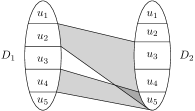
Figure 3: Example of edges between two consecutive cliques $B_{1}$ and $B_{2}$ in a vertex-cycle ${\cal C}_{i}$, where $V_{i}=\{u_{1},\dots,u_{5}\}$. Each region marked with $u_{b}$ in $B_{1}$ and $B_{2}$ contains vertices corresponding to edges of $E_{ij}\subseteq E(G)$ incident to $u_{b}$. Thus, the vertices from the region $u_{b}$ in $B_{1}$ are connected to the vertices of regions $u_{b^{\prime}}$ in $B_{2}$ for all $b^{\prime}>b$. For simplicity, we depicted only edges incident to regions $b_{2}$ and $b_{4}$ in $B_{1}$ .

We introduce a vertex-cycle ${\cal C}_{i}$ for every vertex $i$ of $J$, note that each primary clique $C_{ij}$ is in exactly two vertex-cycles: ${\cal C}_{i}$ and ${\cal C}_{j}$. The number of all base cliques is

$$k:=\underbrace{|E(J)|}_{\begin{subarray}{c}\text{primary}\\ \text{cliques}\end{subarray}}+\underbrace{\sum\nolimits_{i\in V(J)}\deg_{J}(i)\cdot s}_{\text{secondary cliques}}=|E(J)|\cdot\Bigl{(}1+\frac{s}{2}\Bigr{)}\leq\frac{3\ell}{2}\cdot\Bigl{(}1+\frac{s}{2}\Bigr{)}=\mathcal{O}(\ell).$$

This concludes the construction of $(G^{\prime},k)$. Since $V(G^{\prime})$ is partitioned into $k$ base cliques, $k$ is an upper bound on the size of any independent set in $G^{\prime}$, and a solution of size $k$ contains exactly one vertex from each base clique.

We claim that the graph $G^{\prime}$ is in the class $\mathcal{C}^{*}([4,z],5)$. Moreover, if $\operatorname{val}(\Gamma)=1$, then the graph $G^{\prime}$ has an independent set of size $k$ and if the graph $G^{\prime}$ has an independent set of size at least $(1-\gamma^{\prime})\cdot k$ for $\gamma^{\prime}=\frac{\gamma}{6+3s}$, then $\text{val}(\Gamma)\geq 1-\gamma$. By Theorem 5.2, we conclude Theorem 5.1 holds for the class $\mathcal{C}^{*}([4,z],5)$.

Now, we will prove our claims about $G^{\prime}$. For two distinct base cliques $B_{1},B_{2}$, by $E(B_{1},B_{2})$ we denote the set of edges with one endvertex in $B_{1}$ and another in $B_{2}$. We say that $B_{1},B_{2}$ are adjacent if $E(B_{1},B_{2})\neq\emptyset$.

Claim 5.1.

Let $B_{1},B_{2}$ be two distinct base cliques in $G^{\prime}$. Then the size of a maximum induced matching in the graph induced by $E(B_{1},B_{2})$ is at most 1.

Proof.

If $E(B_{1},B_{2})$ is empty, then the lemma holds trivially. Consider two disjoint edges $e=v_{1}v_{2}$ and $e^{\prime}=v^{\prime}_{1}v^{\prime}_{2}$ in $E(B_{1},B_{2})$, where $v_{1},v^{\prime}_{1}\in B_{1}$ and $v_{2},v^{\prime}_{2}\in B_{2}$. We prove that there is an edge $f\in E(B_{1},B_{2})$ such that $f$ intersect both $e$ and $e^{\prime}$.

By construction, $B_{1}$ and $B_{2}$ are consecutive cliques in a vertex-cycle ${\cal C}_{i}$ for some $i\in V(J)$. Assume that $B_{2}$ is the successor of $B_{1}$ on this cycle. Recall that each $v\in\{v_{1},v^{\prime}_{1},v_{2},v^{\prime}_{2}\}$ represents some vertex $r_{i}(v)\in V_{i}$. Since $v_{1}v_{2},v^{\prime}_{1}v^{\prime}_{2}\in E(G^{\prime})$, we observe that $r_{i}(v_{1})\prec_{i}r_{i}(v_{2})$ and $r_{i}(v^{\prime}_{1})\prec_{i}r_{i}(v^{\prime}_{2})$. Thus, at least one of the following holds $r_{i}(v_{1})\prec_{i}r_{i}(v^{\prime}_{2})$ or $r_{i}(v^{\prime}_{1})\prec_{i}r_{i}(v_{2})$. Therefore, at least one of the edges $v_{1}v^{\prime}_{2}$ or $v^{\prime}_{1}v_{2}$ exists in $G^{\prime}$. ∎

Claim 5.2.

The graph $G^{\prime}$ is $(C_{4},\dots,C_{z})$-free.

Proof.

For contradiction, suppose that there exists an induced cycle $K$ in $G^{\prime}$ with consecutive vertices $(v_{1},v_{2},\ldots,v_{p})$, where $p\in[4,z]$. Note that two consecutive vertices of $K$ might be in the same base clique, or two adjacent base cliques. Furthermore, no non-consecutive vertices of $K$ may be in one base clique.

Note that each vertex-cycle in $G^{\prime}$ has at least $2s+2>z$ base cliques. Moreover, if $K$ contains vertices of more than on vertex-cycle, then it has to contains a vertices of at least 4 primary cliques. Thus, the the length of $K$ would be larger than $4s+4>z$. Therefore, we conclude that $K$ cannot intersect more than two base cliques. It cannot intersect one base clique, as $p>3$, so suppose that $K$ intersects exactly two base cliques $B_{1}$ and $B_{2}$. Observe that this means that $p=4$ and $v_{1},v_{2}\in B_{1}$, while $v_{3},v_{4}\in B_{2}$. However, by Claim 5.1, we observe that either $v_{1}$ and $v_{3}$, or $v_{2}$ and $v_{4}$, are adjacent in $G^{\prime}$, so $K$ is not induced. ∎

Claim 5.3.

The graph $G^{\prime}$ is $K_{1,5}$-free.

Proof.

By contradiction suppose that the set $\{v,v_{1},v_{2},v_{3},v_{4},v_{5}\}\subseteq V(G^{\prime})$ induces a copy of $K_{1,5}$ in $G^{\prime}$ with $v$ being the central vertex. Let $B$ be the base clique containing $v$. Since each of $v_{1},v_{2},v_{3},v_{4},v_{5}$ must be in a different base clique and $B$ is adjacent to at most four other base cliques, we conclude that one of $v_{a}$’s, say $v_{5}$, belongs to $B$. For $a\in[4]$, let $B_{i}$ be the base clique containing $u_{a}$. Furthermore, note that $B$ must be a primary clique, say $B=C_{ij}$, since only those ones are adjacent to four base cliques. Therefore two of $B_{a}$’s, say $B_{1}$ and $B_{2}$, must belong to the vertex-cycle ${\cal C}_{i}$. Let $B_{1}$ precede $B$, and $B_{2}$ succeed $B$ on this cycle. Consider the vertices $r_{i}(v),r_{i}(v_{1}),r_{i}(v_{2}),r_{i}(v_{5})$ and recall that since $v$ is adjacent to $v_{1},v_{2}$, we have $r_{i}(v_{1})\prec_{i}r_{i}(v)\prec_{i}r_{i}(v_{2})$. However, $v_{5}$ is non-adjacent to $v_{1},v_{2}$, which means that $r_{i}(v_{2})\prec_{i}r_{i}(v_{5})\prec_{i}r_{i}(v_{1})$, which is a contradiction, since $\prec_{i}$ is transitive. ∎

Claim 5.4.

Let $T\in{\cal T}(s)$. Then, the graph $G^{\prime}$ is $T$-free.

Proof.

Suppose that $G^{\prime}$ contains $T$ as an induced subgraph. Let $v,v^{\prime}\in V(T)$ such that $\deg_{T}(v),\deg_{T}(v^{\prime})\geq 3$ and $\text{dist}_{T}(v,v^{\prime})\leq s$. Note that any two primary cliques are at distance at least $s+1$. Thus, $v$ and $v^{\prime}$ can not be both in primary cliques. Without loss of generality, let $v$ be in a secondary clique $D$ of a vertex-cycle ${\cal C}_{i}$. There are only two base cliques $B_{1}$ and $B_{2}$ adjacent to the secondary clique $D$. Let $v_{1},v_{2}$ and $v_{3}$ be distinct neighbors of $v$ in $T$. Since $v_{1},v_{2}$, and $v_{3}$ form an independent set in $T$, they have to be in distinct base cliques in $G$. Thus, we can suppose $v_{1}\in V(B_{1}),v_{2}\in V(B_{2})$ and $v_{3}\in V(D)$. However, by the same argument as in proof of Claim 5.3 these four vertices $v,v_{1},v_{2}$, and $v_{3}$ cannot exist. ∎

Claim 5.5.

If $\operatorname{val}(\Gamma)=1$, then the graph $G^{\prime}$ has an independent set of size $k$.

Proof.

Let $\phi$ be a solution of $\Gamma$ of value 1, i.e., for each $ij\in E(J)$ holds that $\phi(i)\phi(j)$ is an edge of $G$. We will find an independent set $I$ in $G^{\prime}$ of size $k$. For each $ij\in E(J)$ we add to the set $I$ the vertex from the primary clique $C_{ij}$ which represents the edge $\phi(i)\phi(j)$. Thus, we pick one vertex from each primary clique. Recall that each secondary clique $D$ is a copy of some primary clique $C$. If we pick a vertex $v$ from $C$, then we add to $I$ also a copy of $v$ from $D$. Thus, we add one vertex from each base clique to the set $I$ and therefore $|I|=k$.

We claim that $I$ is independent. Suppose there exist $v,v^{\prime}\in I$ such that $vv^{\prime}\in E(G^{\prime})$. Let $v\in V(B_{1})$ and $v^{\prime}\in V(B_{2})$ for some base cliques $B_{1}$ and $B_{2}$. First, suppose that $B_{1}$ and $B_{2}$ are copies of the same primary clique $C_{ij}$ (or one of them is the primary clique itself and the second one is the copy). Thus, the vertices $v$ and $v^{\prime}$ represent the same edge in $E_{ij}$ and by construction, vertices in primary and secondary cliques representing the same edge in $E_{ij}$ are not adjacent.

Therefore $B_{1}=D^{s}_{ij_{1}}$ and $B_{2}=C_{ij_{2}}$ (or vice versa) for some edges $ij_{1}$ and $ij_{2}$ in $E(J)$. Edges between $B_{1}$ and $B_{2}$ were added according to the ordering $\prec_{i}$ of vertices in $V_{i}$. Note that the vertices $v$ and $v^{\prime}$ represent edges $\phi(i)\phi(j_{1})$ and $\phi(i)\phi(j_{2})$. Thus, $r_{i}(v)=\phi(i)=r_{i}(w)$. Since $v$ and $v^{\prime}$ are adjacent in $G^{\prime}$, it holds that $r_{i}(v)\prec_{i}r_{i}(v^{\prime})$ by construction, which is a contradiction with $r_{i}(v)=r_{i}(v^{\prime})$. Therefore, $I$ is an independent set. ∎

Claim 5.6.

Let $\gamma>0$. If the graph $G^{\prime}$ has an independent set of size at least $(1-\gamma^{\prime})\cdot k$ for $\gamma^{\prime}=\frac{\gamma}{6+3s}$, then $\text{val}(\Gamma)\geq 1-\gamma$.

Proof.

Let

• $I$ be a maximum independent set of $G^{\prime}$ of size at least $(1-\gamma^{\prime})\cdot k$,

• $i$ be a vertex of $J$, and suppose its degree is 3 (the case of vertices of smaller degree is treated analogously),

• $j_{1},j_{2},j_{3}$ be the neighbors of $i$ in $J$,

• $I_{i}$ be an intersection of $I$ and vertices of cliques in ${\cal C}_{i}$.

Suppose that $|I_{i}|=3s+3$, i.e., $I$ intersects each clique in ${\cal C}_{i}$. Let $v_{1},v_{2},v_{3}$ be vertices of intersections of $I$ and $C_{ij_{1}}$, $C_{ij_{2}}$, and $C_{ij_{3}}$, respectively. We claim that $r_{i}(v_{1})=r_{i}(v_{2})=r_{i}(v_{3})$.

Denote the consecutive cliques of ${\cal C}_{i}$ by $B_{1},B_{2},\ldots,B_{3s+3}$. Recall that two cliques in ${\cal C}_{i}$ are adjacent if and only if they are consecutive. For $p\in[3s+3]$ let $v^{\prime}_{p}$ be the unique vertex in $I\cap V(B_{p})$. Define a relation $\succeq_{i}$ on $V_{i}$, such that $v\succeq_{i}v^{\prime}$ iff $v\not\prec_{i}v^{\prime}$. Since $\prec_{i}$ is a total order on $V_{i}$, we have that $v\succeq_{i}v^{\prime}$ iff $v^{\prime}\prec_{i}v$ or $v=v^{\prime}$. Since $v^{\prime}_{1},\dots,v^{\prime}_{3s+3}$ are pairwise nonadjacent, it holds that $r_{i}(v^{\prime}_{1})\succeq_{i}r_{i}(v^{\prime}_{2})\succeq_{i}\dots\succeq_{i}r_{i}(v^{\prime}_{3s+3})\succeq_{i}r_{i}(v^{\prime}_{1})$ by construction. This implies that all vertices $v^{\prime}_{p}$ represent the same vertex $u\in V_{i}$, in particular, $r_{i}(v_{1})=r_{i}(v_{2})=r_{i}(v_{3})=u$.

Now, if $|I_{i}|=3s+3$, we define $\phi(i)=u$ (where $u$ is as in the previous paragraph). If $|I_{i}|<3s+3$ we define $\phi(i)$ arbitrarily. Vertices $i^{\prime}\in V(J)$ of degree 2 are processed similarly, however the size of $I_{i^{\prime}}$ is compared to value $2s+2$. We say that the set $I_{i}$ is complete if $|I_{i}|=(s+1)\cdot\deg(i)$. Thus, if $I_{i}$ and $I_{j}$ are complete, then $\phi(i)\phi(j)$ is an edge of $G$.

Let $Q\subseteq V(J)$ be a set of vertices $i$ of $J$ such that $I_{i}$ is not complete. Note that a primary clique $C_{ij}$ is in two vertex-cycles of base cliques ${\cal C}_{i}$ and ${\cal C}_{j}$ and each secondary clique is in exactly one vertex-cycle of base cliques. Since there are fewer than $\gamma^{\prime}\cdot k$ base cliques $B$ such that $I\cap B=\emptyset$, the set $Q$ has size less than $2\gamma^{\prime}\cdot k$. The vertices in $Q$ are incident to at most $6\gamma^{\prime}\cdot k$ edges in $J$, and all remaining edges of $J$ are satisfied by $\phi$. Therefore,

$$\text{val}(\Gamma)\geq\frac{|E(J)|-6\gamma^{\prime}\cdot k}{|E(J)|}=1-6\gamma^{\prime}\cdot\Bigl{(}1+\frac{s}{2}\Bigr{)}=1-\gamma.\qed$$

This completes the proof of Theorem 5.1 in this case.

5.2 Hardness for $(C_{5}\ldots,C_{z},K_{1,4})$-free Graphs

In this section we show Theorem 5.1 for $\mathcal{C}([5,z],4)$, i.e., for $(C_{5}\ldots,C_{z},K_{1,4})$-free graphs. The proof is similar to the case of $\mathcal{C}^{*}([4,z],5)$. Let $\Gamma=(G,V_{1},\dots,V_{\ell},J)$ be an instance of MCSI(3), we will create an instance $(G^{\prime},k)$ of Independent Set, where $G^{\prime}\in\mathcal{C}(5,z,4)$. Consider an edge $ij$ of $J$. We introduce four primary cliques $C^{1}_{ij},C^{2}_{ij},C^{3}_{ij},C^{4}_{ij}$, each of size $|E_{ij}|$. For each $q\in[4]$, each vertex $v$ of $C^{q}_{ij}$ represents one edge in $E_{ij}$, denote this edge by $r^{\prime}(v)$.

For each $q\in[4]$, we create $s:=\lceil(z-3)/4\rceil$ copies of $C^{q}_{ij}$, denoted by $D^{q,1}_{ij},\ldots,D^{q,s}_{ij}$. Each vertex of a copy represents the same edge as the corresponding vertex in $C^{q}_{ij}$. The cliques created in this step will be called cycle cliques. Again, we imagine that the primary and cycle cliques are arranged in a cyclic way and constitute the edge-cycle corresponding to $ij$:

$$C^{1}_{ij},D^{1,1}_{ij},\ldots,D^{1,s}_{ij},C^{2}_{ij},D^{2,1}_{ij},\ldots,D^{2,s}_{ij},C^{3}_{ij},D^{3,1}_{ij},\ldots,D^{3,s}_{ij},C^{4}_{ij},D^{4,1}_{ij},\ldots,D^{4,s}_{ij},C^{1}_{ij}.$$

Note that all cliques in the edge-cycle are identical. We fix some arbitrary ordering $\prec_{ij}$ on $E_{ij}$, For each two consecutive cliques $B_{1}$ and $B_{2}$ of the edge-cycle, where $B_{1}$ precedes $B_{2}$, and for any vertex $v_{1}$ from $B_{1}$ and any vertex $v_{2}$ from $B_{2}$, we make $v_{1}v_{2}$ adjacent in $G^{\prime}$ if and only if $r^{\prime}(v_{1})\prec_{ij}r^{\prime}(v_{2})$.

After repeating the previous step for every edge $ij$ of $J$, we arrive at the point that $G^{\prime}$ consists of separate edge-cycles, one for each edge of $J$. Since $J$ has maximum degree 3, each edge of $J$ intersects at most 4 other edges. So for each pair of intersecting edges $ij$ and $ij^{\prime}$ we can assign a pair of primary cliques, one in the edge-cycle corresponding to $ij$, and the other one in the edge-cycle corresponding to $ij^{\prime}$, so that no primary clique is assigned twice.

Consider two edges of $J$, that share a vertex, say edges $ij$ and $ij^{\prime}$, and suppose the primary cliques chosen in the last step are $C^{p}_{ij}$ and $C^{q}_{ij^{\prime}}$. We need to provide some connection between these cliques, to make the choices for edges $ij$ and $ij^{\prime}$ consistent. Let us arbitrarily choose one of cliques $C^{p}_{ij}$ and $C^{q}_{ij^{\prime}}$, say $C^{p}_{ij}$, and create $s$ copies of it, denote these cliques by $F^{1}_{ijj^{\prime}},F^{2}_{ijj^{\prime}},\ldots,F^{s}_{ijj^{\prime}}$ (again, the represented edges are inherited from the primary clique). We call these cliques equality cliques. We build an equality gadget by arranging these cliques in a sequence as follows:

$$C^{p}_{ij},F^{1}_{ijj^{\prime}},F^{2}_{ijj^{\prime}},\ldots,F^{s}_{ijj^{\prime}},C^{q}_{ij^{\prime}}.$$

Consider two consecutive cliques $B_{1}$ and $B_{2}$ of this sequence, except for the last pair. These cliques are identical. Between them we add edges that form an antimatching, i.e., for a vertex $v_{1}$ of $B_{1}$ and a vertex $v_{2}$ of $B_{2}$, we add an edge $v_{1}v_{2}$ if and only if $r^{\prime}(v_{1})\neq r^{\prime}(v_{2})$. Finally, for a vertex $v_{1}$ of $F^{s}_{ijj^{\prime}}$ and a vertex $v_{2}$ of $C^{q}_{ij}$, we add an edge $v_{1}v_{2}$ if and only if $r^{\prime}(v_{1})\cap r^{\prime}(v_{2})\neq\emptyset$, i.e., edges represented by these vertices contain different vertices from $V_{i}$.

This completes the construction of $G^{\prime}$. By base cliques we mean primary cliques, cycle cliques, and equality cliques. Let $k$ be the number of all base cliques, i.e.,

$$k:=\underbrace{4|E(J)|}_{\begin{subarray}{c}\text{primary}\\ \text{cliques}\end{subarray}}+\underbrace{4s|E(J)|}_{\begin{subarray}{c}\text{cycle}\\ \text{cliques}\end{subarray}}+\underbrace{\sum_{i\in V(J)}\binom{\deg_{J}(i)}{2}\cdot s}_{\text{equality cliques}}=\mathcal{O}(\ell).$$

Let us upper-bound $k$. If $\ell_{2}$ and $\ell_{3}$ are, respectively, the numbers of vertices of $J$ with degree 2 and 3, then we obtain

$$k=4|E(J)|(s+1)+s(\ell_{2}+3\ell_{3})\leq\frac{9s}{2}\cdot|E(J)|+4\leq 5s\cdot|E(J)|.$$ (1)

The following claim is proven in an analogous way to Claim 5.2, note that this time we might obtain induced copies of $C_{4}$, where two vertices are in an equality clique, and the other two are in a different base clique in the same equality gadget (either an equality clique or a primary clique).

Claim 5.7.

The graph $G^{\prime}$ is $(C_{5},\dots,C_{z})$-free.

The next claim is in turn analogous to Claim 5.3.

Claim 5.8.

The graph $G^{\prime}$ is $K_{1,4}$-free.

Proof.

Observe that each clique is adjacent to at most three other cliques, and the only cliques adjacent to three other cliques are primary cliques. So if we hope to find an induced $K_{1,4}$, the center and one leaf must be in a primary clique, say $C^{q}_{ij}$, and other three leaves are in distinct base cliques adjacent to $C^{q}_{ij}$. However, two of cliques adjacent to $C^{q}_{ij}$ must belong to the same edge-cycle (and the third one is an equality clique). Similarly as in the proof of Claim 5.3, we observe that the leaf that belongs to $C^{q}_{ij}$ must be adjacent to at least one of the remaining leaves. ∎

The following claims are analogous to the corresponding claims in Section 5.1. Therefore we provide only sketches of proofs.

Claim 5.9.

If $\operatorname{val}(\Gamma)=1$, then the graph $G^{\prime}$ has an independent set of size $k$.

Proof.

Consider a solution $\phi$ of $\Gamma$ of value 1. Therefore, for each $ij\in E(J)$, the pair $\phi(i)\phi(j)$ is an edge of $G$. Note that this edge is represented by some $v$ in each primary clique $C^{q}_{ij}$. We select those vertices to the set $I$. Recall that each remaining clique $B$ (i.e., a cycle clique or an equality clique), is a copy of some primary clique $C$. For each such clique $B$ we include to $I$ the vertex, which is a copy of the selected vertex in $C$.

By an argument analogous to the one in the proof of Claim 5.5 we observe that the selected vertices belonging to one edge-cycle are pairwise non-adjacent. Furthermore, note that the edges between adjacent cliques in an equality gadget are defined in a way, so that all selected vertices from cliques in this gadget are pairwise non-adjacent. Thus, the $I$ is an independent set of size $k$. ∎

Claim 5.10.

Let $\gamma>0$. If the graph $G^{\prime}$ has an independent set of size at least $(1-\gamma^{\prime})\cdot k$ for $\gamma^{\prime}=\frac{\gamma}{45s}$, then $\text{val}(\Gamma)\geq 1-\gamma$.

Proof.

Consider an independent set $I$ in $G$ of size at least $(1-\gamma^{\prime})\cdot k$, and a vertex $i\in V(J)$. Suppose that $\deg(i)=3$ and the neighbors of $i$ in $J$ are $j_{1},j_{2},j_{3}$ (if the degree of $i$ is smaller, the reasoning is analogous).

Let $\mathcal{S}^{i}$ be the union of all base cliques corresponding to $i$, i.e.,

1. belonging to edge-cycles corresponding to $ij_{1},ij_{2},ij_{3}$, and

2. belonging to equality gadgets between these edge-cycles.

Note that the number of cliques in $\mathcal{S}^{i}$ is $3\cdot 4(s+1)+3\cdot s=15s+12$, and let $I_{i}$ be the intersection of $I$ with the vertices of $\mathcal{S}^{i}$. Suppose that the size of $I_{i}$ is $15s+12$, i.e., we selected a vertex from each base clique in $\mathcal{S}^{i}$ – we call such $I_{i}$ complete. By the reasoning analogous to Claim 5.6, we observe that for each of three edge-cycles in $\mathcal{S}^{i}$, the selected vertices correspond to the same edge of $G$, denote these edges by $e_{1},e_{2},e_{3}$, respectively. Furthermore, as in the proof of Claim 5.9, we observe that the edges $e_{1},e_{2},e_{3}$ share a vertex $v\in V_{i}$. If $I_{i}$ is complete, we set $\phi(i)=v$. Otherwise, we set $\phi(i)$ arbitrarily.

Let $Q$ be the set of those $i$, for which $I_{i}$ is not complete. We observe that each base clique $B$ is in at most three sets $\mathcal{S}^{i}$. Consider a base clique $B$. If $B$ is a primary clique or a cycle clique, then it corresponds to some $E_{ij}$, and $B$ belongs $\mathcal{S}^{i}$ and $\mathcal{S}^{j}$. In the last case, if $B$ is an equality clique in the equality gadget joining edge-cycles corresponding to, say, $ij_{1}$ and $ij_{2}$, then $C$ belongs to $\mathcal{S}^{i},\mathcal{S}^{j_{1}},\mathcal{S}^{j_{2}}$. Summing up, each base clique belongs to at most three sets $\mathcal{S}^{i}$. Since there are fewer than $\gamma^{\prime}\cdot k$ base cliques $B$, such that $B\cap I=\emptyset$, we observe that the size of $Q$ is at most $3\gamma^{\prime}\cdot k$. The vertices in $Q$ are incident to at most $9\gamma^{\prime}\cdot k$ edges in $J$, and all remaining edges are satisfied by $\phi$. So, using (1), we obtain

$$\operatorname{val}(\Gamma)\geq\frac{|E(J)|-9\gamma^{\prime}\cdot k}{|E(J)|}\geq 1-45s\cdot\gamma^{\prime}=1-\gamma.\qed$$

5.3 Refuting Constant-Factor FPT Approximation

In this section we prove Theorem 1.6. However, as mentioned in Section 1, we need to consider a larger class than $\mathcal{C}^{*}([4,z],5)$ to obtain the lower bound. Let ${\cal P}(a,b)$ be a graph family consisting of cycles $C_{p}$ for all $p\in[a,b]$ and all trees without twins in ${\cal T}(\lceil\frac{b-1}{2}\rceil)$ and let $\mathcal{D}(a,b)$ be the class of ${\cal P}(a,b)$-free graphs. Note that $\mathcal{C}^{*}([a,b],c)\subseteq{\cal D}(a,b)$ as ${\cal P}(a,b)\subseteq\mathcal{H}([a,b],c)\cup{\cal T}(\lceil\frac{b-1}{2}\rceil)$. We will prove the following theorem that implies Theorem 1.6.

Theorem 5.3.

Let $z\geq 5$ be a constant. Let $\gamma>0$ be a constant and let $f:\mathbb{N}\to\mathbb{N}$ be a computable function. Unless the deterministic Gap-ETH fails, there is no algorithm, given an $n$-vertex instance $G\in\mathcal{D}(5,z)$ and an integer $k$, runs in time $f(k)\cdot n^{\mathcal{O}(1)}$ and can distinguish between the two cases: $\alpha(G)\geq k$, and $\alpha(G)<(1-\gamma)\cdot k$.

The idea of the proof is to use the lexicographic product to amplify the approximation factor given by statement (2) of Theorem 5.1. Let $G_{1}=(V_{1},E_{1})$ and $G_{2}=(V_{2},E_{2})$ be graphs. The lexicographic product $G_{1}\times_{\ell}G_{2}$ is the graph $G=(V,E)$ such that $V=V_{1}\times V_{2}$ and $(u_{1},v_{1})(u_{2},v_{2})\in E$ if $u_{1}u_{2}\in E_{1}$ or $u_{1}=u_{2}$ and $v_{1}v_{2}\in E_{2}$. In other words, the graph $G$ consist of copies $G^{u}_{2}$ of $G_{2}$, one for each $u\in V_{1}$, and a vertex $v_{1}$ from $G^{u_{1}}_{2}$ and a vertex $v_{2}$ from $G^{u_{2}}_{2}$ (for $u_{1}\neq u_{2}$) are adjacent if and only if $u_{1}u_{2}\in E_{1}$. We use the following two properties of the lexicographic product to obtain our result.

Proposition 3 (Geller and Stahl [26]).

For graphs $G_{1},G_{2}$, it holds that $\alpha(G_{1}\times_{\ell}G_{2})=\alpha(G_{1})\cdot\alpha(G_{2})$.

Unfortunately, the lexicographic product does not preserve “$H$-freeness” for all graphs $H\in\mathcal{H}([a,b],c)\cup{\cal T}(b^{\prime})$. Indeed, it might contain a copy of $H$ even if the original graphs were $H$-free. However, this might happen only if $H$ has some specific structure, as shown in the next proposition. Note that no graph in $\mathcal{H}([a,b],c)$ and ${\cal T}(b^{\prime})$ contains a triangle and they are all connected.

Proposition 4.

Let $H$ be connected, triangle-free graph without twins. Let $G_{1}$ and $G_{2}$ be $H$-free graphs. Then, $G_{1}\times_{\ell}G_{2}$ is also $H$-free.

Proof.

Suppose for a contradiction that $G=G_{1}\times_{\ell}G_{2}$ contains $H$ as an induced subgraph. As we mentioned above, $G$ consists of copies $G^{u}_{2}$ of $G_{2}$ for each $u\in V_{1}$. First, the copy of $H$ cannot be completely contained in one copy $G^{u}_{2}$ as $G_{2}$ is $H$-free. Supose that each copy $G^{u}_{2}$ contains at most one vertex of $H$. Then, the graph $G_{1}$ would contain $H$ as an induced subgraph. Thus, there is a copy $G^{u_{1}}_{2}$ that contains at least two vertices of $H$, say $w_{1}=(u_{1},v_{2})$ and $w_{2}=(u_{1},v_{2})$.

The graph $H$ has no twins and the neighbors of $w_{1}$ and $w_{2}$ outside of $G^{u_{1}}_{2}$ are the same. Thus, there is another vertex $w_{3}=(u_{1},v_{3})$ of $H$ in $G^{u_{1}}_{2}$ such that $w_{3}$ is adjacent to one of the vertices $w_{1}$ and $w_{2}$, without loss of generality say $w_{1}$. Since the graph $H$ is connected and is not entirely contained in $G^{u_{1}}_{2}$, there is a vertex $w_{4}=(u_{2},v^{\prime})$ of $H$ in $G^{u_{2}}_{2}$ such that $w_{4}$ is adjacent to at least one vertex of $w_{1},w_{2},w_{3}$. However, since at least one edge is present between $G^{u_{1}}_{2}$ and $G^{u_{2}}_{2}$, there is an edge $u_{1}u_{2}\in E(G_{2})$ and therefore, there is a complete bipartite graph between $G^{u_{1}}_{2}$ and $G^{u_{2}}_{2}$. Thus, $w_{4}$ is connected to all $w_{1},w_{2}$, and $w_{3}$. Since $H$ is an induced subgraph of $G$, the graph $H$ would contain a triangle $w_{1},w_{3},w_{4}$, which is a contradiction. ∎

When we restrict the family $\mathcal{C}([4,b],c)$ to the graphs without twins we get exactly a family consisting of cycles of length at least 5 and at most $b$, as cycles of length at least 5 do not contain twins and on the other hand the stars and $C_{4}$ contain twins. Hence, by restricting the family $\mathcal{C}^{*}([4,z],5)$ (as used in Theorem 5.1) to the graphs without twins we obtain exactly the family ${\cal P}(5,z)$. Note that graphs in $\mathcal{C}([5,z],4)$ without twins are in ${\cal P}(5,z)$ as well.

Proof of Theorem 5.3.

Suppose for a contradiction there is a constant $\gamma_{0}>0$ and an algorithm $\mathcal{A}$ with runtime $f(k)\cdot n^{c}$ for a computable function $f$ and a constant $c$ that for an input graph $G\in\mathcal{D}(5,z)$ can distinguish between two cases whether $\alpha(G)\geq k$ or $\alpha(G)<(1-\gamma_{0})\cdot k$. Let $\gamma$ be a constant given by statement (2) of Theorem 5.1. Recall that $\mathcal{C}^{*}([4,z],5)\subseteq\mathcal{D}(5,z)$. Thus in particular, there is no algorithm with runtime $f(k)\cdot n^{\mathcal{O}(1)}$ that can distinguish between the cases whether $\alpha(G)\geq k$ or $\alpha(G)<(1-\gamma)\cdot k$ (under the deterministic Gap-ETH).

Let $d$ be the smallest integer such that $(1-\gamma)^{d}\leq(1-\gamma_{0})$. Now, let $G^{d}$ be a $d$-fold lexicographic product of $G$ with itself, i.e.,

$$G^{d}=\underbrace{G\times_{\ell}\dots\times_{\ell}G}_{d}.$$

Recall that each graph in ${\cal P}(5,z)$ is connected, triangle-free and without twins, thus by Proposition 4, $G^{d}\in\mathcal{D}(5,z)$ as well. Further by Proposition 3, $\alpha(G^{d})=\alpha(G)^{d}$. Now consider the two cases listed in the statement. If $\alpha(G)\geq k$, then $\alpha(G^{d})\geq k^{d}$. On the other hand, if $\alpha(G)<(1-\gamma)\cdot k$, then $\alpha(G^{d})<(1-\gamma)^{d}\cdot k^{d}\leq(1-\gamma_{0})\cdot k^{d}$ by the definition of $d$. Thus, the algorithm $\mathcal{A}$ would distinguish the cases whether $\alpha(G^{d})\geq k^{d}$ or $\alpha(G^{d})<(1-\gamma_{0})\cdot k^{d}$ in time $f(k^{d})\cdot n^{c}$. Subsequently, we can distinguish between the cases whether $\alpha(G)\geq k$ or $\alpha(G)\leq(1-\gamma)\cdot k$ in time $f(k^{d})\cdot(n^{d})^{c}=f^{\prime}(k)\cdot n^{\mathcal{O}(1)}$ for a computable function $f^{\prime}$, which is a contradiction with statement (2) of Theorem 5.1. ∎

6 Parameterized Approximation with $H$ as a Parameter

In this section we still consider the Independent Set problem in $H$-free graphs, but now our parameter is related to the graph $H$. First, we show Proposition 1. We point out that a similar argument was also observed by Bonnet [5].

See 1

Proof.

We will reduce from Multicolored Independent Set, for which the vertices of the input graph are partitioned into $k$ disjoint sets $V_{1},V_{2}\ldots,V_{k}$, each of which forms a clique. Note that any independent set can contain at most one vertex from each set $V_{i}$ where $i\in\{1,\ldots,k\}$. Let $\mathcal{H}_{d}$ be a class of graphs as in the statement. Set $k=d$ and let $G$ be an instance of Multicolored Independent Set. Let us observe that the vertex set of $G$ is partitioned into $k=d$ cliques, so $G$ is clearly $H$-free for every $H\in\mathcal{H}_{d}$.

By simply taking the complement of the input graph, we can easily establish that Multicolored Independent Set is as hard as MCSI where $J$ is a clique, i.e., the Multicolored Clique problem. Thus Multicolored Independent Set is W[1]-hard and has no $n^{o(k)}$ algorithm, unless the ETH fails [15, Theorem 13.25 and Corollary 14.23]. Furthermore, by a result of Lin et al. [33] the Multicolored Clique problem has no $k^{o(1)}$-approximation in $f(k)n^{O(1)}$ time under ETH, and by Chalermsook et al. [9] no clique of size $\zeta(k)$ can be computed in $f(k)n^{\zeta(k)}$ time under the deterministic Gap-ETH. From these results the statement follows. ∎

Now let us consider the Independent Set problem in $K_{1,d}$-free graphs, parameterized by both $k$ and $d$. In this case we are able to give parameterized approximation lower bounds based on the following sparsification of MCSI.

Theorem 6.1.

Consider an instance $\Gamma=(G,V_{1},\dots,V_{\ell},J)$ of MCSI($t$) with size $n$. Let $\xi(\ell)=2^{(\log\ell)^{1/2+\varepsilon}}$ for any constant $0<\varepsilon<1/2$, and let $\zeta$ be any function in $\omega(1)$. Given that $t>\xi(\ell)$ or $t>\zeta(\ell)$, respectively, for any computable function $f$, there is no $f(\ell)\cdot n^{\mathcal{O}(1)}$ time algorithm that can distinguish between the two cases:

1. (YES-case) $\operatorname{val}(\Gamma)=1$, and

2. (NO-case)

   • $\operatorname{val}(\Gamma)\leq\xi(\ell)/t$ assuming the deterministic Gap-ETH, and

   • $\operatorname{val}(\Gamma)\leq\zeta(\ell)/t$ assuming the Strongish Planted Clique Hypothesis.

To prove Theorem 6.1 we need two facts. The first is the Erdős-Gallai theorem on degree sequences, which are sequences of non-negative integers $d_{1},\ldots,d_{n}$, for each of which there exists a simple graph on $n$ vertices such that vertex $i\in[n]$ has degree $d_{i}$. We use the following constructive formulation due to Choudum [12].

Theorem 6.2 (Erdős-Gallai theorem [12]).

A sequence of non-negative integers $d_{1}\geq\dots\geq d_{n}$ is a degree sequence of a simple graph on $n$ vertices if $d_{1}+\dots+d_{n}$ is even and for every $1\leq k\leq n$ the following inequality holds:
$\sum_{i=1}^{k}d_{i}\leq k(k-1)+\sum_{i=k+1}^{n}\min(d_{i},k).$ Moreover, given such a degree sequence, a corresponding graph can be constructed in polynomial time.

We also need parameterized approximation lower bounds for MCSI, as given by Dinur and Manurangsi [17] and Manurangsi et al. [39].

Theorem 6.3 (Dinur and Manurangsi [17], Manurangsi et al. [39]).

Consider an instance $\Gamma=(G,V_{1},\dots,V_{\ell},J)$ of MCSI with size $n$ and $J$ a complete graph. Let $\xi(\ell)=2^{(\log\ell)^{1/2+\varepsilon}}$ for any constant $0<\varepsilon<1/2$, and let $\zeta$ be any function in $\omega(1)$. There is no $f(\ell)\cdot n^{\mathcal{O}(1)}$ time algorithm for any computable function $f$ that can distinguish between the following two cases:

1. (YES-case) $\operatorname{val}(\Gamma)=1$, and

2. (NO-case)

   • $\operatorname{val}(\Gamma)\leq\xi(\ell)/{\ell}$ under the deterministic Gap-ETH, and

   • $\operatorname{val}(\Gamma)\leq\zeta(\ell)/{\ell}$ under the Strongish Planted Clique Hypothesis.

Proof of Theorem 6.1.

Let $\Gamma=(G,V_{1},\dots,V_{\ell},J)$ be an instance of MCSI where $J$ is a complete graph. To find an instance of MCSI($t$) given $\Gamma$, we first need to construct a graph $J^{\prime}$ with maximum degree $t$, for which we use the Erdős-Gallai theorem. For this, let $\ell^{\prime}=\ell$ if $\ell$ is even and $\ell^{\prime}=\ell-1$ if $\ell$ is odd. Now, by Theorem 6.2 it is easy to verify that a $t$-regular graph on $\ell^{\prime}$ vertices exists as $t\ell^{\prime}$ is even. Moreover, the proof of Theorem 6.2 by Choudum [12] is constructive, so that we can compute $J^{\prime}$ on $\ell$ vertices in polynomial time by setting it to the constructed $t$-regular graph if $\ell^{\prime}=\ell$, or by adding one more isolated vertex if $\ell^{\prime}=\ell-1$. Note that $V(J^{\prime})=V(J)=\{1,\ldots,\ell\}$, $E(J^{\prime})\subseteq E(J)$ as $J$ is a complete graph, and $|E(J^{\prime})|=t\ell^{\prime}/2$.

We create a graph $G^{\prime}$ by removing edges from $G$ according to $J^{\prime}$. That is, for any $1\leq i,j\leq\ell$, if $ij\not\in E(J^{\prime})$ then we remove all edges between sets $V_{i}$ and $V_{j}$. The resulting subgraph of $G$ is called $G^{\prime}$, and we get an instance $\Gamma^{\prime}=(G^{\prime},V_{1},\dots,V_{\ell},J^{\prime})$ of MCSI($t$).

It is easy to see that if $\text{val}(\Gamma)=1$, then $\text{val}(\Gamma^{\prime})=1$ as well: we just use the optimal solution for $\Gamma$ and remove any edges non-existent in $G^{\prime}$. Now suppose that $\text{val}(\Gamma)\leq\nu$, which means that every solution $\phi$ satisfies at most a $\nu$-fraction of edges of $J$. Let $\phi$ be an arbitrary solution of $\Gamma^{\prime}$, which is also a solution for $\Gamma$ as $G^{\prime}\subseteq G$ and $J^{\prime}\subseteq J$. By our assumption we know that it satisfies at most $\nu\cdot|E(J)|$ edges of $J$. Thus, the solution $\phi$ satisfies at most $\nu\cdot|E(J)|$ edges of $J^{\prime}$ as well, and we obtain

$$\operatorname{val}(\Gamma^{\prime})\leq\frac{\nu\cdot|E(J)|}{|E(J^{\prime})|}=\nu\cdot\frac{\ell(\ell-1)/2}{t\ell^{\prime}/2}\leq\nu\cdot\frac{\ell(\ell-1)}{t(\ell-1)}=\nu\cdot\frac{\ell}{t}.$$

By the first part of Theorem 6.3, no $f(\ell)\cdot n^{\mathcal{O}(1)}$ time algorithm can distinguish between $\operatorname{val}(\Gamma)=1$ and $\operatorname{val}(\Gamma)\leq{\xi(\ell)}/{\ell}$ given $\Gamma$, where $\xi(\ell)=2^{(\log k)^{1/2+\varepsilon}}$ for any constant $0<\varepsilon<1/2$, under the deterministic Gap-ETH. By the above calculations, for $\Gamma^{\prime}$ we obtain that no such algorithm can distinguish between $\operatorname{val}(\Gamma^{\prime})=1$ and $\operatorname{val}(\Gamma^{\prime})\leq\xi(\ell)/t$ by setting $\nu={\xi(\ell)}/{\ell}$, and so we obtain the first part of Theorem 6.1.

When using the second part of Theorem 6.3 instead, under the Strongish Planted Clique Hypothesis, given $\Gamma$ and any function $\zeta\in\omega(1)$, no $f(\ell)\cdot n^{\mathcal{O}(1)}$ time algorithm can distinguish between $\operatorname{val}(\Gamma)=1$ and $\operatorname{val}(\Gamma)\leq{\zeta(\ell)}/{\ell}$. Analogous to before, we obtain the second part of Theorem 6.1 by setting $\nu=\zeta(\ell)/\ell$. ∎

Based on Theorem 6.1 we can prove Proposition 2 using the reduction of Lemma 1.

See 2

Proof.

We reduce via Lemma 1 from MCSI($t$) to Independent Set, which given an instance $\Gamma$ of MCSI($t$) results in a $K_{1,2t+2}$-free graph $G$ for Independent Set. We thus set $d=2t+2$. If $\operatorname{val}(\Gamma)=1$, then $G$ has an independent set of size $k={\ell\choose 2}$. If $\operatorname{val}(\Gamma)\leq\xi(\ell)/t$ or $\operatorname{val}(\Gamma)\leq\zeta(\ell)/t$, then every independent set of $G$ has size at most $\xi(\ell){\ell\choose 2}/t\leq\frac{\xi(k)k}{d/2-1}$ or $\zeta(\ell){\ell\choose 2}/t\leq\frac{\zeta(k)k}{d/2-1}$, respectively, assuming w.l.o.g. that $k\geq 4$ so that $\ell\leq 2\sqrt{k}\leq k$. In the first case, given a constant $\varepsilon^{\prime}>0$ we may choose $\varepsilon$ small enough in Theorem 6.1 so that $\frac{\xi(k)k}{d/2-1}\leq 2^{(\log k)^{1/2+\varepsilon^{\prime}}}k/d$. Thus, for $\xi^{\prime}(k)=2^{(\log k)^{1/2+\varepsilon^{\prime}}}$, a $d/\xi^{\prime}(k)$-approximation algorithm for Independent Set would be able to distinguish between the YES- and NO-case of $\Gamma$. In the second case, given any function $\zeta^{\prime}\in\omega(1)$, we may choose an appropriate function $\zeta\in\omega(1)$ in Theorem 6.1 for which $\frac{\zeta(k)k}{d/2-1}\leq\zeta^{\prime}(k)k/d$. Thus a $d/\zeta^{\prime}(k)$-approximation algorithm for Independent Set would be able to distinguish between the YES- and NO-case of $\Gamma$.

Note that $d=2t+2\leq 2\ell$ as the maximum degree of the graph $J$ is $\ell-1$. Thus if the runtime of this algorithm is $f(d,k)\cdot n^{\mathcal{O}(1)}$, then for some function $f^{\prime}$ this would be a $f^{\prime}(\ell)\cdot n^{\mathcal{O}(1)}$ time algorithm for MCSI($t$). However, according to Theorem 6.1 this would be a contradiction, unless the deterministic Gap-ETH or the Strongish Planted Clique Hypothesis fails, respectively. We may rename $\xi^{\prime}(k)$ to $\xi(k)$ or $\zeta^{\prime}(k)$ to $\zeta(k)$ to obtain Proposition 2. ∎

7 Conclusion and Open Problems

Our parameterized inapproximability results of Theorem 1.5 suggest that the Independent Set problem is hard to approximate to within some constant, whenever it is W[1]-hard to solve on $H$-free graphs, according to Theorem 1.2. In most cases it is unclear though whether any approximation can be computed (either in polynomial time or by exploiting the parameter $k$), which beats the strong lower bounds for polynomial-time algorithms for general graphs. The only known exceptions to this are the $K_{1,d}$-free case, where a polynomial-time $(\frac{d-1}{2}+\delta)$-approximation algorithm was shown by Halldórsson [28], and the $K_{a,b}$-free case, for which we showed a polynomial-time $\mathcal{O}\bigl{(}(a+b)^{1/a}\cdot\alpha(G)^{1-1/a}\bigr{)}$-approximation algorithm in Theorem 1.3. For $K_{1,d}$-free graphs, we were also able to show an almost asymptotically tight lower bound for polynomial-time algorithms in Theorem 1.4. For parameterized algorithms, our lower bound of Proposition 2 for $K_{1,d}$-free graphs does not give a tight bound, but seems to suggest that parameterizing by $k$ does not help to obtain an improvement.

Settling the question whether $H$-free graphs admit better approximations to Independent Set than general graphs, remains a challenging open problem, both for polynomial-time algorithms and algorithms exploiting the parameter $k$.

Let us point out one more, concrete open question. Recall from Theorem 1.2 Bonnet et al. [6] were able to show W[1]-hardness for graphs which simultanously exclude $K_{1,4}$ and all induced cycles of length in $[4,z]$, for any constant $z\geq 5$. On the other hand, we presented two separate reductions, one for $(K_{1,5},C_{4},\ldots,C_{z})$-free graphs, and another one for $(K_{1,4},C_{5},\ldots,C_{z})$-free graphs. It would be nice to provide a uniform reduction, i.e., prove hardness for parameterized approximation in $(K_{1,4},C_{4},\ldots,C_{z})$-free graphs.

Finally, note that the statement (3) of Theorem 5.2 only excludes algorithms with running time $f(k)\cdot n^{o(\sqrt{k})}$. However, a straightforward algorithm has running time $f(k)\cdot n^{\mathcal{O}(k)}$. Is is possible to obtain a matching lower bound (at least up to polylogarithmic factors in the exponent)?

8 Acknowledgement

We would like to thank to the anonymous reviewer, who suggested using gap amplification to obtain Theorem 1.6. We are also grateful to the other reviewer for pointing out the mistake in Theorem 1.5 in the conference version of our paper [19].

References

- [1] V. Alekseev. Polynomial algorithm for finding the largest independent sets in graphs without forks. Discrete Applied Mathematics, 135(1):3 – 16, 2004. Russian Translations II.
- [2] V. E. Alekseev. The effect of local constraints on the complexity of determination of the graph independence number. Combinatorial-algebraic methods in applied mathematics, pages 3–13, 1982.
- [3] P. Austrin, S. Khot, and M. Safra. Inapproximability of vertex cover and independent set in bounded degree graphs. Theory of Computing, 7(1):27–43, 2011.
- [4] N. Bansal, A. Gupta, and G. Guruganesh. On the Lovász theta function for independent sets in sparse graphs. SIAM Journal on Computing, 47(3):1039–1055, 2018.
- [5] É. Bonnet. private communication.
- [6] É. Bonnet, N. Bousquet, P. Charbit, S. Thomassé, and R. Watrigant. Parameterized complexity of independent set in h-free graphs. Algorithmica, 82(8):2360–2394, 2020.
- [7] É. Bonnet, N. Bousquet, S. Thomassé, and R. Watrigant. When maximum stable set can be solved in FPT time. In 30th International Symposium on Algorithms and Computation, ISAAC 2019, December 8-11, 2019, Shanghai University of Finance and Economics, Shanghai, China, pages 49:1–49:22, 2019.
- [8] É. Bonnet, S. Thomassé, X. T. Tran, and R. Watrigant. An algorithmic weakening of the erdős-hajnal conjecture. In F. Grandoni, G. Herman, and P. Sanders, editors, 28th Annual European Symposium on Algorithms, ESA 2020, September 7-9, 2020, Pisa, Italy (Virtual Conference), volume 173 of LIPIcs, pages 23:1–23:18. Schloss Dagstuhl - Leibniz-Zentrum für Informatik, 2020.
- [9] P. Chalermsook, M. Cygan, G. Kortsarz, B. Laekhanukit, P. Manurangsi, D. Nanongkai, and L. Trevisan. From gap-exponential time hypothesis to fixed parameter tractable inapproximability: Clique, dominating set, and more. SIAM Journal on Computing, 49(4):772–810, 2020.
- [10] S. O. Chan. Approximation resistance from pairwise-independent subgroups. Journal of the ACM (JACM), 63(3):1–32, 2016.
- [11] R. Chitnis, A. E. Feldmann, and P. Manurangsi. Parameterized approximation algorithms for bidirected Steiner Network problems, 2017.
- [12] S. Choudum. A simple proof of the Erdős-Gallai theorem on graph sequences. Bulletin of the Australian Mathematical Society, 33(1):67–70, 1986.
- [13] M. Chudnovsky, M. Pilipczuk, M. Pilipczuk, and S. Thomassé. Quasi-polynomial time approximation schemes for the maximum weight independent set problem in H-free graphs. In Proceedings of the 2020 ACM-SIAM Symposium on Discrete Algorithms, SODA 2020, Salt Lake City, UT, USA, January 5-8, 2020, pages 2260–2278, 2020.
- [14] D. Corneil, H. Lerchs, and L. Burlingham. Complement reducible graphs. Discrete Applied Mathematics, 3(3):163 – 174, 1981.
- [15] M. Cygan, F. V. Fomin, L. Kowalik, D. Lokshtanov, D. Marx, M. Pilipczuk, M. Pilipczuk, and S. Saurabh. Parameterized Algorithms. Springer, 2015.
- [16] K. Dabrowski, V. V. Lozin, H. Müller, and D. Rautenbach. Parameterized algorithms for the independent set problem in some hereditary graph classes. In Combinatorial Algorithms - 21st International Workshop, IWOCA 2010, London, UK, July 26-28, 2010, Revised Selected Papers, pages 1–9, 2010.
- [17] I. Dinur and P. Manurangsi. ETH-hardness of approximating 2-CSPs and Directed Steiner Network. In 9th Innovations in Theoretical Computer Science Conference, ITCS 2018, January 11-14, 2018, Cambridge, MA, USA, pages 36:1–36:20, 2018.
- [18] I. Dinur and P. Manurangsi. ETH-hardness of approximating 2-CSPs and Directed Steiner Network. CoRR, abs/1805.03867, 2018.
- [19] P. Dvořák, A. E. Feldmann, A. Rai, and P. Rzążewski. Parameterized inapproximability of independent set in h-free graphs. In I. Adler and H. Müller, editors, Graph-Theoretic Concepts in Computer Science - 46th International Workshop, WG 2020, Leeds, UK, June 24-26, 2020, Revised Selected Papers, volume 12301 of Lecture Notes in Computer Science, pages 40–53. Springer, 2020.
- [20] P. Erdős and G. Szekeres. A Combinatorial Problem in Geometry, pages 49–56. Birkhäuser Boston, Boston, MA, 1987.
- [21] U. Feige. Approximating maximum clique by removing subgraphs. SIAM J. Discrete Math., 18(2):219–225, 2004.
- [22] U. Feige, S. Goldwasser, L. Lovász, S. Safra, and M. Szegedy. Interactive proofs and the hardness of approximating cliques. J. ACM, 43(2):268–292, 1996.
- [23] A. E. Feldmann, Karthik C. S., E. Lee, and P. Manurangsi. A survey on approximation in parameterized complexity: Hardness and algorithms. Algorithms, 13(6):146, 2020.
- [24] M. Garey, D. Johnson, and L. Stockmeyer. Some simplified NP-complete graph problems. Theoretical Computer Science, 1(3):237 – 267, 1976.
- [25] P. Gartland and D. Lokshtanov. Independent set on -free graphs in quasi-polynomial time. In IEEE 61st Annual Symposium on Foundations of Computer Science (FOCS), pages 613–624, 2020.
- [26] D. Geller and S. Stahl. The chromatic number and other functions of the lexicographic product. Journal of Combinatorial Theory, Series B, 19(1):87–95, 1975.
- [27] A. Grzesik, T. Klimošová, M. Pilipczuk, and M. Pilipczuk. Polynomial-time algorithm for maximum weight independent set on P-free graphs. ACM Trans. Algorithms, 18(1):4:1–4:57, 2022.
- [28] M. M. Halldórsson. Approximating discrete collections via local improvements. In Proceedings of the Sixth Annual ACM-SIAM Symposium on Discrete Algorithms, 22-24 January 1995. San Francisco, California, USA, pages 160–169, 1995.
- [29] J. Håstad. Clique is hard to approximate within . In Acta Mathematica, pages 627–636, 1996.
- [30] R. M. Karp. Reducibility among combinatorial problems. In Complexity of Computer Computations, pages 85–103. Springer US, 1972.
- [31] S. Khot and A. K. Ponnuswami. Better inapproximability results for Max Clique, Chromatic Number and Min-3Lin-Deletion. In M. Bugliesi, B. Preneel, V. Sassone, and I. Wegener, editors, Automata, Languages and Programming, pages 226–237, Berlin, Heidelberg, 2006. Springer Berlin Heidelberg.
- [32] B. Laekhanukit. Parameters of two-prover-one-round game and the hardness of connectivity problems. In Proceedings of the twenty-fifth annual ACM-SIAM symposium on Discrete algorithms (SODA), pages 1626–1643. SIAM, 2014.
- [33] B. Lin, X. Ren, Y. Sun, and X. Wang. On Lower Bounds of Approximating Parameterized k-Clique. In 49th International Colloquium on Automata, Languages, and Programming (ICALP 2022), volume 229, pages 90:1–90:18, 2022.
- [34] D. Lokshantov, M. Vatshelle, and Y. Villanger. Independent set in P-free graphs in polynomial time. In Proceedings of the Twenty-Fifth Annual ACM-SIAM Symposium on Discrete Algorithms, SODA 2014, Portland, Oregon, USA, January 5-7, 2014, pages 570–581, 2014.
- [35] D. Lokshtanov, M. S. Ramanujan, S. Saurabh, and M. Zehavi. Parameterized complexity and approximability of directed odd cycle transversal. In Proceedings of the Thirty-First Annual ACM-SIAM Symposium on Discrete Algorithms, SODA ’20, page 2181–2200, USA, 2020. Society for Industrial and Applied Mathematics.
- [36] V. V. Lozin and M. Milanič. A polynomial algorithm to find an independent set of maximum weight in a fork-free graph. J. Discrete Algorithms, 6(4):595–604, 2008.
- [37] K. Majewski, T. Masařík, J. Novotná, K. Okrasa, M. Pilipczuk, P. Rzążewski, and M. Sokołowski. Max weight independent set in graphs with no long claws: An analog of the gyárfás’ path argument. In M. Bojanczyk, E. Merelli, and D. P. Woodruff, editors, 49th International Colloquium on Automata, Languages, and Programming, ICALP 2022, July 4-8, 2022, Paris, France, volume 229 of LIPIcs, pages 93:1–93:19. Schloss Dagstuhl - Leibniz-Zentrum für Informatik, 2022.
- [38] P. Manurangsi. Tight running time lower bounds for strong inapproximability of maximum k-coverage, unique set cover and related problems (via t-wise agreement testing theorem). In Proceedings of the 2020 ACM-SIAM Symposium on Discrete Algorithms, SODA 2020, Salt Lake City, UT, USA, January 5-8, 2020, pages 62–81, 2020.
- [39] P. Manurangsi, A. Rubinstein, and T. Schramm. The Strongish Planted Clique Hypothesis and Its Consequences. In 12th Innovations in Theoretical Computer Science Conference (ITCS 2021), volume 185 of Leibniz International Proceedings in Informatics (LIPIcs), pages 10:1–10:21, 2021.
- [40] D. Marx. Can you beat treewidth? Theory of Computing, 6(1):85–112, 2010.
- [41] D. Marx and M. Pilipczuk. Optimal parameterized algorithms for planar facility location problems using voronoi diagrams. ACM Trans. Algorithms, 18(2):13:1–13:64, 2022.
- [42] G. J. Minty. On maximal independent sets of vertices in claw-free graphs. Journal of Combinatorial Theory, Series B, 28(3):284 – 304, 1980.
- [43] M. Pilipczuk, M. Pilipczuk, and P. Rzążewski. Quasi-polynomial-time algorithm for independent set in -free graphs via shrinking the space of induced paths. In H. V. Le and V. King, editors, 4th Symposium on Simplicity in Algorithms, SOSA 2021, Virtual Conference, January 11-12, 2021, pages 204–209. SIAM, 2021.
- [44] S. Poljak. A note on stable sets and colorings of graphs. Commentationes Mathematicae Universitatis Carolinae, 15:307–309, 1974.
- [45] N. Sbihi. Algorithme de recherche d’un stable de cardinalite maximum dans un graphe sans etoile. Discrete Mathematics, 29(1):53 – 76, 1980.