Low-Rank Autoregressive Tensor Completion for Multivariate Time Series Forecasting

Abstract

Time series prediction has been a long-standing research topic and an essential application in many domains. Modern time series collected from sensor networks (e.g., energy consumption and traffic flow) are often large-scale and incomplete with considerable corruption and missing values, making it difficult to perform accurate predictions. In this paper, we propose a low-rank autoregressive tensor completion (LATC) framework to model multivariate time series data. The key of LATC is to transform the original multivariate time series matrix (e.g., sensor$\times$time point) to a third-order tensor structure (e.g., sensor$\times$time of day$\times$day) by introducing an additional temporal dimension, which allows us to model the inherent rhythms and seasonality of time series as global patterns. With the tensor structure, we can transform the time series prediction and missing data imputation problems into a universal low-rank tensor completion problem. Besides minimizing tensor rank, we also integrate a novel autoregressive norm on the original matrix representation into the objective function. The two components serve different roles. The low-rank structure allows us to effectively capture the global consistency and trends across all the three dimensions (i.e., similarity among sensors, similarity of different days, and current time v.s. the same time of historical days). The autoregressive norm can better model the local temporal trends. Our numerical experiments on three real-world data sets demonstrate the superiority of the integration of global and local trends in LATC in both missing data imputation and rolling prediction tasks.

1 Introduction

Time series prediction serves as the foundation for a wide range of real-world applications and decision-making processes. Although the field of time series analysis has been developed for a long time, traditional time series models (e.g., autoregressive (AR), ARIMA, exponential smoothing) mainly focus on parametric models for small-scale problems [1]. However, the structure and properties of emerging “big” time series data have posed new challenges [2]. In particular, modern time series data collected from field applications and sensor networks are often large-scale (e.g., time series from thousands of sensors), high-dimensional (e.g., matrix/tensor-variate sequences [3, 4]), and incomplete (even sparse) with considerable corruption and missing values. A critical challenge is to perform efficient and reliable predictions for large-scale time series with missing values [5].

The fundamental of modeling of modern large-scale, high-dimensional time series is to effectively characterize the complex dependencies and correlations across different dimensions. Spatiotemporal data is an excellent example with complex dependencies/correlations across both spatial and temporal dimensions [6]. Taking traffic flow time series collected from a network of sensors as an example, we often observe clear spatial consistency (e.g., nearby sensors generate similar readings) and both long-term and short-term temporal trends and correlations [7]. To model both long-term and short-term correlations, various neural sequence models have been developed [8, 9, 10, 11]. However, these models cannot effectively deal with the missing data problem, and most of them requiring performing imputation as a preprocessing step, which may introduce potential bias. How to incorporate long-term/short-term patterns and sensor correlation in the presence of missing data remains an important research question.

To address data incompleteness, dimensionality reduction methods such as matrix/tensor factorization have been applied to model multivariate and high-order (matrix/tensor-variate) time series data [3, 5, 12, 4, 13]. To acquire prediction power, it is essential for these factorization-based models to impose certain time series structures on the latent layer. However, real-world time series data often have complex temporal structures beyond the simple AR model, exhibiting patterns at different scales and resolutions (weekly, daily, and hourly). For example, human behavior related time series (e.g., household energy consumption and highway traffic flow data) often simultaneously demonstrate long-term patterns at the daily and weekly levels and short-term perturbations. Clearly, these short-term and long-term patterns are critical to prediction tasks. Potential solutions to accommodate both of them are to introduce kernel structures in Gaussian process [14] and to use the Hankel transformation following singular spectrum analysis and Hankel structured low-rank models [15, 16]; however, the computational cost makes it challenging for large (number of sensors) and long (number of time points) multivariate time series data.

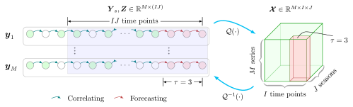
Figure 1: Illustration of the proposed LATC imputer/predictor with a prediction window $\tau$ (green nodes: observed values; white nodes: missing values; red nodes/panel: prediction; blue panel: training data to construct the tensor). For example, if $\boldsymbol{Y}$ captures hourly traffic flow and the goal is perform prediction for the next $\tau=3$ hours, we can set $I=24$ and choose $J$ accordingly.

In this paper, we propose a low-rank autoregressive tensor completion (LATC) framework to model large-scale multivariate time series with missing values. In LATC, the original multivariate time series matrix is transformed to a third-order tensor based on the most important seasonality, and thus both missing data imputation and future value prediction problems can be naturally translated to a universal tensor completion problem (see Figure 1). To achieve better prediction power, we use tensor nuclear norm minimization and truncated nuclear norm minimization to preserve the long-term/global trends. We then define a new autoregressive norm on the original matrix representation to characterize short-term/local trends. With this approach, all the observed data in tensor $\boldsymbol{\mathcal{X}}$ will contribute to the final prediction (i.e., the red panel in Figure 1). We evaluate LATC on three real-world data sets for both missing data imputation and rolling prediction tasks, and compare it with several state-of-the-art approaches. Our numerical experiments show encouraging performance of LATC, suggesting that the model can effectively capture both global and local trends in time series data.

2 Related work

In this paper, we focus on developing low-rank models for large-scale multivariate time series data in the presence of missing values. Essentially, there are three types of approaches for this problem.

Temporal factorization Low-rank completion is a popular technique for collaborative filtering and missing data imputation. Some recent studies have used low-rank models for multivariate and high-order time series data [3, 5, 4, 11, 13]. Essentially, these models require a well-designed generative mechanism on the temporal latent layer to achieve smoothing and to harness prediction power. For example, AR models are used to regularize factor matrix and core tensors in [5, 13] and [4]. However, these models essentially only capture the global consistency/similarity among different time series, but they cannot effectively accommodate the global trends (daily/weekly patterns) on the temporal dimension. Therefore, a critical challenge is to design an effective temporal model, since AR might be too limited to capture periodic pattern at different scales.

Hankel/delay embedding Singular spectrum analysis (SSA) and Hankel structured low-rank completion are powerful approaches for time series analysis [15, 16]. They are model-free approaches to detect spectral patterns at different scales in time series data. Essentially, SSA applies singular value decomposition (SVD) on the Hankel matrix obtained from the original univariate time series, and then uses those principle components to analyze the time series. The default SSA model is for univariate time series but it can be easily extended to the multivariate case. This approach can accomplish both missing data imputation and prediction tasks by performing low-rank completion on the Hankel matrix [17, 18, 19, 20, 21, 22]. However, such model is computationally expensive to model the Hankel matrices/tensors. It might be infeasible to deal with large and long multivariate time series.

Tensor representation Another approach is to fold a time series matrix into a tensor by introducing an additional “season” dimension (e.g., a third-order tensor with a “day” dimension). In fact, many real-world time series data resulted from human behavior/activities (e.g., traffic flow, customer demand, electricity consumption) exhibit both long-term and short-term patterns. Recent studies have used the tensor representation [sensor$\times$day$\times$time of day] to capture the patterns (e.g., [23, 24, 25, 26]). The tensor representation also offers prediction ability by performing tensor completion [24, 25]. The tensor representation not only preserves the dependencies among sensors but also provides a new alternative to capture both local and global temporal patterns. These models have shown superiority over matrix-based models in missing data imputation tasks [26].

3 Preliminaries

Notations

We use boldface uppercase letters to denote matrices, e.g., $\boldsymbol{X}\in\mathbb{R}^{M\times N}$, boldface lowercase letters to denote vectors, e.g., $\boldsymbol{x}\in\mathbb{R}^{M}$, and lowercase letters to denote scalars, e.g., $x$. Given a multivariate time series matrix $\boldsymbol{X}\in\mathbb{R}^{M\times N}$ ($M$ sensors over $N$ time points), we use $\boldsymbol{X}_{[:t]}\in\mathbb{R}^{M\times t}$ and $\boldsymbol{X}_{[t+1:]}\in\mathbb{R}^{M\times(N-t)}$ to denote the submatrices of $\boldsymbol{X}$ that consist of the first $t$ columns and the last $N-t$ columns, respectively. Let $\boldsymbol{X}_{[t_{1}:t_{2}]}\in\mathbb{R}^{M\times(t_{2}-t_{1}+1)}$ denote the submatrix of $\boldsymbol{X}$ formed by columns $t_{1}$ to $t_{2}$ and $\boldsymbol{x}_{t}$ denote the vector at time $t$. We denote the $(m,n)$th entry in $\boldsymbol{X}$ by $x_{m,n}$. The Frobenius norm of $\boldsymbol{X}$ is defined as $\|\boldsymbol{X}\|_{F}=\sqrt{\sum_{m,n}x_{m,n}^{2}}$. The nuclear norm (NN) is defined as $\|\boldsymbol{X}\|_{*}=\sum_{i=1}^{\min\{M,N\}}\sigma_{i}$, where $\sigma_{i}$ denotes the $i$th largest singular value of $\boldsymbol{X}$. The truncated nuclear norm (TNN) of $\boldsymbol{X}$ is defined as the sum of the $\left(\min\{M,N\}-\theta\right)$ smallest singular values, i.e., $\|\boldsymbol{X}\|_{\theta,*}=\sum_{i=\theta+1}^{\min\{M,N\}}\sigma_{i}$. The $\ell_{2}$-norm of $\boldsymbol{x}$ is defined as $\|\boldsymbol{x}\|_{2}=\sqrt{\sum_{m}x_{m}^{2}}$. We denote a third-order tensor by $\boldsymbol{\mathcal{X}}\in\mathbb{R}^{M\times I\times J}$ and the $k$th-mode ($k=1,2,3$) unfolding of $\boldsymbol{\mathcal{X}}$ by $\boldsymbol{\mathcal{X}}_{(k)}$ [27]. Correspondingly, we define a folding operator that converts a matrix to a third-order tensor in the $k$th-mode as $\operatorname{fold}_{k}(\cdot)$; thus, we have $\operatorname{fold}_{k}(\boldsymbol{\mathcal{X}}_{(k)})=\boldsymbol{\mathcal{X}}$.

Low-rank matrix/tensor completion

The low-rank matrix completion (LRMC) model imposes an underlying low-rank structure to recover an incomplete matrix. Given a partially observed matrix $\boldsymbol{Y}\in\mathbb{R}^{M\times N}$ with an index set $\Omega$ of observed entries, LRMC can be formulated as:

$$\min_{\boldsymbol{X}}{} \operatorname{rank}(\boldsymbol{X})$$ (1)

s.t. $$\mathcal{P}_{\Omega}(\boldsymbol{X})=\mathcal{P}_{\Omega}(\boldsymbol{Y}),$$

where $\boldsymbol{X}$ is the recovered matrix. The symbol $\operatorname{rank}(\cdot)$ denotes the rank of a given matrix. The operator $\mathcal{P}_{\Omega}:\mathbb{R}^{M\times N}\mapsto\mathbb{R}^{M\times N}$ is an orthogonal projection supported on $\Omega$:

$$[\mathcal{P}_{\Omega}(\boldsymbol{X})]_{m,n}=\left\{\begin{array}[]{ll}x_{m,n},&\text{if $(m,n)\in\Omega$,}\\ 0,&\text{otherwise}.\\ \end{array}\right.$$

Problem (1) is NP-hard. A convex relaxation is to use $\|\boldsymbol{X}\|_{*}$ as a surrogate for the rank function [28]. Low-rank tensor completion (LRTC) extends LRMC to higher-order tensors. Ref. [29] defines the tensor nuclear norm as the weighted sum of NNs of all the unfolded matrices, i.e., $\|\boldsymbol{\cal{X}}\|_{*}=\sum_{k}\alpha_{k}\|\boldsymbol{\cal{X}}_{(k)}\|_{*}$, where $\alpha_{k}$s are non-negative weight parameters with $\sum_{k}\alpha_{k}=1$.

Autoregressive model of time series

Autoregressive model is a standard statistical model for time series. Given a time series matrix $\boldsymbol{X}\in\mathbb{R}^{M\times N}$, the vector autoregressive (VAR) model gives

$$\boldsymbol{x}_{t}=\sum_{i}\boldsymbol{A}_{i}\boldsymbol{x}_{t-h_{i}}+{\epsilon}_{t},$$ (2)

where $\mathcal{H}=\{h_{1},\ldots,h_{d}\}$ is a set of time lags, $\boldsymbol{A}_{i}$ is a coefficients matrix for lag $h_{i}$, and $\epsilon_{mt}$s are Gaussian noises. VAR can capture the dependencies among different time series, but in the meanwhile it has a large number of parameters $M\times M\times d$. We can also model each individual time series follows an independent autoregressive model as ${x}_{m,t}=\sum_{i}{a}_{m,i}{x}_{m,t-h_{i}}+{\epsilon}_{m,t}$, and this reduces the coefficients to a matrix $\boldsymbol{A}=[a_{m,i}]\in\mathbb{R}^{M\times d}$.

4 Low-rank autoregressive tensor completion

In this section, we introduce the low-rank autoregressive tensor completion (LATC) framework to impute missing values and predict future values of a multivariate time series matrix $\boldsymbol{Y}$. The setting of LATC is essentially the same as in TRMF [5] and BTMF [13]. The two models introduce an autoregressive regularizer (on the temporal factor matrix $\boldsymbol{X}$) to characterize temporal dynamics when factorizing matrix $\boldsymbol{Y}\approx\boldsymbol{F}\boldsymbol{X}$. The learned autoregressive regularizer enables us perform prediction on the temporal factor matrix $\boldsymbol{X}$ to get $\boldsymbol{X}_{\text{new}}$, and then the final prediction can be obtained by $\boldsymbol{Y}_{\text{new}}=\boldsymbol{F}\boldsymbol{X}_{\text{new}}$. A fundamental challenge in factorization-based time series models is to design the structural model to effectively capture both long-term and short-term temporal dependencies.

The key idea of the proposed LATC model is to transform the matrix-based prediction/imputation problem to a universal low-rank tensor completion problem (see the illustration in Figure 1). Our main motivation to transform the time series matrix to a tensor is that many real-world time series, such as traffic flow and energy consumption data, are characterized by both long-term/global trends and short-term/local trends [7]. The long-term trends refer to certain periodic, seasonal, and cyclical patterns. For example, traffic flow data over 24 hours on a typical weekday often shows a systematic “M” shape resulted from travelers’ behavioral rhythms, with two peaks during morning and evening rush hours [9]. The pattern also exists at the weekly level with substantial differences from weekdays to weekends. The short-term trends capture certain temporary volatility/perturbation that deviates from the global patterns (e.g., due to incident/event). The short-term trends seem more “random”, but they are common and ubiquitous in reality. LATC leverages both global and local patterns by using a tensor structure. As shown in Figure 1, the first step of LATC is to convert the multivariate time series matrix $\boldsymbol{Y}$ into a tensor. We define an operator $\mathcal{Q}(\cdot)$, which converts the multivariate time series matrix into a third-order tensor. For instance, a partially observed matrix $\boldsymbol{Y}\in\mathbb{R}^{M\times(IJ)}$ can be converted into tensor $\mathcal{Q}(\boldsymbol{Y})\in\mathbb{R}^{M\times I\times J}$. Note that, given the size constraint, not all values are in $\boldsymbol{Y}$ to construct the tensor (see Figure 1). Correspondingly, $\mathcal{Q}^{-1}(\cdot)$ denotes the inverse operator that converts the third-order tensor into a multivariate time series matrix.

We define LATC as the following optimization problem:

$$\min_{\boldsymbol{\mathcal{X}},\boldsymbol{Z},\boldsymbol{A}}{} \|\boldsymbol{\mathcal{X}}\|_{*}+\lambda\|\boldsymbol{Z}\|_{\boldsymbol{A},\mathcal{H}}$$ (3)

s.t. $$\left\{\begin{array}[]{l}\boldsymbol{\mathcal{X}}=\mathcal{Q}\left(\boldsymbol{Z}\right),\\ \mathcal{P}_{\Omega}(\boldsymbol{Z})=\mathcal{P}_{\Omega}(\boldsymbol{Y}),\\ \end{array}\right.$$

where $\boldsymbol{Y}\in\mathbb{R}^{M\times(IJ)}$ is the partially observed time series matrix and $\boldsymbol{Z}$ has the same size as $\boldsymbol{Y}$, and $\lambda$ is a weight parameter that controls the trade-off between the two terms in the objective function. We define the autoregressive norm of matrix $\boldsymbol{Z}$ with a lag set $\mathcal{H}$ and coefficient matrix $\boldsymbol{A}$ as:

$$\|\boldsymbol{Z}\|_{\boldsymbol{A},\mathcal{H}}=\sum_{m,t}(z_{m,t}-\sum_{i}a_{m,i}z_{m,t-h_{i}})^{2}.$$ (4)

Note that, with this definition, $\boldsymbol{A}$ is also a variable to estimate. For simplicity, we use independent autoregressive models in Eq. (4) instead of a full vector autoregressive model. To solve the optimization problem, we perform the following transformation by introducing auxiliary variables $\boldsymbol{\mathcal{X}}_{k}$:

$$\min_{\{\boldsymbol{\mathcal{X}}_{k}\}_{k=1}^{3},\boldsymbol{Z},\boldsymbol{A}}{} \sum_{k}\alpha_{k}\|\boldsymbol{\mathcal{X}}_{k(k)}\|_{*}+\lambda\|\boldsymbol{Z}\|_{\boldsymbol{A},\mathcal{H}}$$ (5)

s.t. $$\left\{\begin{array}[]{l}\boldsymbol{\mathcal{X}}_{k}=\mathcal{Q}\left(\boldsymbol{Z}\right),~{}k=1,2,3,\\ \mathcal{P}_{\Omega}(\boldsymbol{Z})=\mathcal{P}_{\Omega}(\boldsymbol{Y}).\\ \end{array}\right.$$

We next show the new optimization problem (5) can be efficiently solved by employing the Alternating Direction Method of Multipliers (ADMM) framework. First, we introduce the following lemma, which allows us to estimate $\boldsymbol{A}$.

Lemma 1.

For two time series matrices $\boldsymbol{Z}=\boldsymbol{X}$ consisting of $M$ time series with $N$ time points, suppose the two variables follow an autoregressive model with a lag set $\mathcal{H}=\{h_{1},\ldots,h_{d}\}$:

$${z}_{m,t}=\sum_{i}{a}_{m,i}{x}_{m,t-h_{i}}+{\epsilon}_{m,t},\forall~{}m,t,$$

with $\epsilon_{mt}$ being Gaussian noise. Let $\boldsymbol{Q}_{m}=(\boldsymbol{v}_{h_{d}+1},\cdots,\boldsymbol{v}_{N})^{\top}\in\mathbb{R}^{(N-h_{d})\times d}$ with $\boldsymbol{v}_{t}=({x}_{m,t-h_{1}},\cdots,{x}_{m,t-h_{d}})^{\top}$. Then, the solution to the problem

$$\min_{\boldsymbol{a}_{m}}~{}\frac{1}{2}\|\boldsymbol{z}_{m,[h_{d}+1:]}-\boldsymbol{Q}_{m}\boldsymbol{a}_{m}\|_{2}^{2}$$

can be written as

$$\hat{\boldsymbol{a}}_{m}:=(\boldsymbol{Q}_{m}^{\top}\boldsymbol{Q}_{m})^{-1}\boldsymbol{Q}_{m}^{\top}\boldsymbol{z}_{m,[h_{d}+1:]}=\boldsymbol{Q}_{m}^{+}\boldsymbol{z}_{m,[h_{d}+1:]},$$ (6)

where $\cdot^{+}$ denotes the pseudo-inverse of matrix.

Therefore, we can write down the following subproblems for ADMM:

$$\boldsymbol{\mathcal{X}}_{k}^{l+1} :=\operatorname{arg}\min_{\boldsymbol{\mathcal{X}}}~{}\alpha_{k}\|\boldsymbol{\mathcal{X}}_{(k)}\|_{*}+\frac{\rho}{2}\|\mathcal{Q}^{-1}(\boldsymbol{\mathcal{X}})-\boldsymbol{Z}^{l}\|_{F}^{2}+\big{\langle}\mathcal{Q}^{-1}(\boldsymbol{\mathcal{X}})-\boldsymbol{Z}^{l},\mathcal{Q}^{-1}(\boldsymbol{\mathcal{T}}_{k}^{l})\big{\rangle},$$ (7)

$$\boldsymbol{Z}^{l+1}_{[:h_{d}]} :=\operatorname{arg}\min_{\boldsymbol{Z}}~{}\sum_{k}\left(\frac{\rho}{2}\|\mathcal{Q}^{-1}(\boldsymbol{\mathcal{X}}_{k}^{l+1})_{[:h_{d}]}-\boldsymbol{Z}\|_{F}^{2}+\big{\langle}\mathcal{Q}^{-1}(\boldsymbol{\mathcal{X}}_{k}^{l+1})_{[:h_{d}]}-\boldsymbol{Z},\mathcal{Q}^{-1}(\boldsymbol{\mathcal{T}}_{k}^{l})_{[:h_{d}]}\big{\rangle}\right),$$ (8)

$$\boldsymbol{Z}^{l+1}_{[h_{d}+1:]} \begin{aligned} &:=\operatorname{arg}\min_{\boldsymbol{Z}}~{}\sum_{m}\frac{\lambda}{2}\|\boldsymbol{z}_{m,[h_{d}+1:]}-\boldsymbol{Q}_{m}\boldsymbol{a}_{m}\|_{2}^{2}+\\ &\sum_{k}\left(\frac{\rho}{2}\|\mathcal{Q}^{-1}(\boldsymbol{\mathcal{X}}_{k}^{l+1})_{[h_{d}+1:]}-\boldsymbol{Z}\|_{F}^{2}+\big{\langle}\mathcal{Q}^{-1}(\boldsymbol{\mathcal{X}}_{k}^{l+1})_{[h_{d}+1:]}-\boldsymbol{Z},\mathcal{Q}^{-1}(\boldsymbol{\mathcal{T}}_{k}^{l})_{[h_{d}+1:]}\big{\rangle}\right)\\ \end{aligned}$$ (9)

$$\boldsymbol{a}_{m}^{l+1} :=\boldsymbol{Q}_{m}^{+}\boldsymbol{z}^{l+1}_{m,[h_{d}+1:]},$$ (10)

$$\boldsymbol{\mathcal{T}}_{k}^{l+1} :=\boldsymbol{\mathcal{T}}_{k}^{l}+\rho(\boldsymbol{\mathcal{X}}_{k}^{l+1}-\mathcal{Q}(\boldsymbol{Z}^{l+1})),$$ (11)

where the symbol $\left<\cdot,\cdot\right>$ denotes the inner product, $\rho$ is the learning rate of ADMM algorithm, and $l$ denotes the count of iteration. The matrix $\boldsymbol{Q}_{m}$ used in Eq. (9) and (10) are defined on the matrix $\mathcal{Q}^{-1}(\hat{\boldsymbol{\mathcal{X}}})$ where $\hat{\boldsymbol{\mathcal{X}}}$ is the estimated tensor at iteration $l+1$: $\hat{\boldsymbol{\mathcal{X}}}=\sum_{k}\alpha_{k}\boldsymbol{\mathcal{X}}_{k}^{l+1}$.

The subproblem (7) for computing $\boldsymbol{\mathcal{X}}_{k}$ is convex, and the closed-form solution is given by

$$\boldsymbol{\mathcal{X}}_{k}^{l+1}:=\operatorname{fold}_{k}\left(\mathcal{D}_{\alpha_{k}/\rho}(\mathcal{Q}(\boldsymbol{Z}^{l})_{(k)}-\boldsymbol{\mathcal{T}}_{k(k)}^{l}/\rho)\right),$$ (12)

where the symbol $\mathcal{D}_{\alpha/\rho}(\cdot)$ denotes the operator of singular value thresholding with shrinkage parameter $\alpha/\rho$. The solution in Eq. (12) meets the singular value thresholding as shown in Lemma 2.

Lemma 2.

For any $\alpha,\rho>0$, and $\boldsymbol{Z}\in\mathbb{R}^{M\times N}$, a global optimal solution to the problem $\min_{\boldsymbol{X}}~{}\alpha\|\boldsymbol{X}\|_{*}+\frac{1}{2}\rho\|\boldsymbol{X}-\boldsymbol{Z}\|_{F}^{2}$ is given by the singular value thresholding [30]:

$$\hat{\boldsymbol{X}}:=\mathcal{D}_{\alpha/\rho}(\boldsymbol{Z})=\boldsymbol{U}\mathop{\mathrm{diag}}\left([\boldsymbol{\sigma}(\boldsymbol{Z})-\alpha/\rho]_{+}\right)\boldsymbol{V}^{\top},$$ (13)

where $\boldsymbol{Z}=\boldsymbol{U}\mathop{\mathrm{diag}}(\boldsymbol{\sigma}(\boldsymbol{Z}))\boldsymbol{V}^{\top}$ is the singular value decomposition of $\boldsymbol{Z}$. The symbol $[\cdot]_{+}$ denotes the positive truncation at 0 which satisfies $[\boldsymbol{\sigma}-\alpha/\rho]_{+}=\max\{\boldsymbol{\sigma}-\alpha/\rho,\boldsymbol{0}\}$.

For variable $\boldsymbol{Z}$, the subproblems (8) and  (9) are both convex least squares. We can therefore derive the closed-form solution

$$\boldsymbol{Z}_{[:h_{d}]}^{l+1}:= \frac{1}{3}\sum_{k}\mathcal{Q}^{-1}(\boldsymbol{\mathcal{X}}_{k}^{l+1}+\boldsymbol{\mathcal{T}}_{k}^{l}/\rho)_{[:h_{d}]},$$ (14)

$$\boldsymbol{z}_{m,[h_{d}+1:]}^{l+1}:= \frac{1}{3(\rho+\lambda)}\sum_{k}\mathcal{Q}^{-1}(\rho\boldsymbol{\mathcal{X}}_{k}^{l+1}+\boldsymbol{\mathcal{T}}_{k}^{l})_{m,[h_{d}+1:]}+\frac{\lambda}{\rho+\lambda}\boldsymbol{Q}_{m}\boldsymbol{a}_{m}^{l},$$ (15)

where we impose a fixed consistency constraint, namely $\mathcal{P}_{\Omega}(\boldsymbol{Z}^{l+1}):=\mathcal{P}_{\Omega}(\boldsymbol{Y})$, to guarantee the transformation of observation information at each iteration. In addition, for Eq. (15), we can set $\lambda$ as $c_{0}\cdot\rho$ with $c_{0}$ being a constant determining the relative weight of time series regression.

Until now, we use the NN in the objective function of LATC. In fact, another way to capture global low-rank patterns is through the TNN minimization, which is experimentally proved to be better than NN minimization [31]. In this paper, we also test a variant of LATC based on TNN minimization, and solve the following subproblem for updating $\boldsymbol{\mathcal{X}}_{k}$:

$$\boldsymbol{\mathcal{X}}_{k}^{l+1}:=\operatorname{arg}\min_{\boldsymbol{\mathcal{X}}}~{}\alpha_{k}\|\boldsymbol{\mathcal{X}}_{(k)}\|_{\theta,*}+\frac{1}{2}\rho\|\mathcal{Q}^{-1}(\boldsymbol{\mathcal{X}})-\boldsymbol{Z}^{l}\|_{F}^{2}+\big{\langle}\mathcal{Q}^{-1}(\boldsymbol{\mathcal{X}})-\boldsymbol{Z}^{l},\mathcal{Q}^{-1}(\boldsymbol{\mathcal{T}}_{k}^{l})\big{\rangle},$$ (16)

where $\theta$ is a nonnegative integer. The TNN minimization reduces to NN minimization when $\theta=0$. Thus, Eq. (7) is indeed a special case of Eq. (16). If we integrate Lemma 3 into Eq. (16), we get

$$\boldsymbol{\mathcal{X}}_{k}^{l+1}:=\operatorname{fold}_{k}\left(\mathcal{D}_{\theta,\alpha_{k}/\rho}(\mathcal{Q}(\boldsymbol{Z}^{l})_{(k)}-\boldsymbol{\mathcal{T}}_{k(k)}^{l}/\rho)\right).$$ (17)

Lemma 3.

For any $\alpha,\rho>0$, $\boldsymbol{Z}\in\mathbb{R}^{M\times N}$, and $\theta\in\mathbb{N}_{+}$ where $\theta<\min\{M,N\}$, an optimal solution to the problem $\min_{\boldsymbol{X}}~{}\alpha\|\boldsymbol{X}\|_{\theta,*}+\frac{1}{2}\rho\|\boldsymbol{X}-\boldsymbol{Z}\|_{F}^{2}$ is given by the generalized singular value thresholding [32, 33, 34]:

$$\hat{\boldsymbol{X}}:=\mathcal{D}_{\theta,\alpha/\rho}(\boldsymbol{Z})=\boldsymbol{U}\mathop{\mathrm{diag}}\left([\boldsymbol{\sigma}(\boldsymbol{Z})-\mathfrak{1}_{\theta}\cdot\alpha/\rho]_{+}\right)\boldsymbol{V}^{\top},$$ (18)

where $\boldsymbol{Z}=\boldsymbol{U}\mathop{\mathrm{diag}}(\boldsymbol{\sigma}(\boldsymbol{Z}))\boldsymbol{V}^{\top}$ is the singular value decomposition of $\boldsymbol{Z}$. The symbol $[\cdot]_{+}$ denotes the positive truncation at 0 as defined in Lemma 2. $\mathfrak{1}_{\theta}\in\{0,1\}^{\min\{M,N\}}$ is a binary indicator vector whose first $\theta$ entries are 0 and other entries are 1.

5 Experiments

5.1 Experiment setup

In this section, we assess the performance of LATC using three real-world multivariate time series data sets: (1) PeMS (P) registers traffic speed time series from 228 sensors over 44 days with 288 time points per day (i.e., 5-min frequency). (2) Guangzhou (G) contains traffic speed time series from 214 road segments in Guangzhou, China over 61 days with 144 time points per day (i.e., 10-min frequency). (3) Electricity (E) records hourly electricity consumption transactions of 370 clients from 2011 to 2014. We use a subset of the last five weeks of 321 clients in our experiments.

Our experiments cover the same two tasks as in [5]: missing data imputation and rolling prediction. As mentioned, in LATC, both imputation and prediction are achieved by performing tensor completion. For missing data imputation, we follow the default LATC framework as a general imputer procedure (see Algorithm 1). The default prediction task follows the description in Figure 1, in which we use the recovered values of the red submatrix as the prediction for the future $\tau$ time points as a window. Rolling prediction for multiple windows is obtained by applying LATC repeatedly. Algorithm 2 summarizes the rolling predictor procedure for $S$ rolling windows.

The sizes $M\times I\times J$ of the transformed tensors of the three data sets are: 228$\times$288$\times$44 for (P), 214$\times$144$\times$61 for (G), and 321$\times$24$\times$35 for (E). For the imputation task, we randomly mask certain amount (20%/40%) of values as missing. We consider two missing scenarios: random missing (RM) in which entries are missing randomly, and non-random missing (NM) in which each time series has block missing for randomly selected days (i.e., randomly removing mode-3 fibers in tensor $\mathcal{Q}(\boldsymbol{Y})$). For data set (P), we perform rolling predictions for the last 5 days (i.e., 1440 time points) with $\tau=9$ and $S=160$ for in the presence of missing values. Similarly, we also predict the last 7 days for data set (G) with $\tau=12$ and $S=84$ and the last 5 days for data set (E) with $\tau=6$ and $S=20$. We use $\text{MAPE}=\frac{1}{n}\sum_{i=1}^{n}|\frac{x_{i}-\hat{x}_{i}}{x_{i}}|\times 100$ and $\text{RMSE}=\sqrt{\frac{1}{n}\sum_{i=1}^{n}\left(x_{i}-\hat{x}_{i}\right)^{2}}$ as performance metrics. The adapted data sets and Python implementation for these experiments are available in our GitHub repository https://github.com/xinychen/tensor-learning.

Initialize $\boldsymbol{\mathcal{T}}$ as zeros and $\boldsymbol{A}$ as small random values. Set $\mathcal{P}_{\Omega}(\boldsymbol{Z})=\mathcal{P}_{\Omega}(\boldsymbol{Y})$ and $l=0$.

while not converged do

       for $k=1$ to $3$ do

             Update $\boldsymbol{\mathcal{X}}_{k}^{l+1}$ by Eq. (12) for NN or Eq. (17) for TNN;

      

      Compute $\hat{\boldsymbol{\mathcal{X}}}=\sum_{k}\alpha_{k}\boldsymbol{\mathcal{X}}_{k}^{l+1}$, and then $\hat{\boldsymbol{X}}=\mathcal{Q}^{-1}(\hat{\boldsymbol{\mathcal{X}}})$;

       Update $\boldsymbol{Z}_{[:h_{d}]}^{l+1}$ by Eq. (14);

       for $m=1$ to $M$ do

             Build $\boldsymbol{Q}_{m}$ on $\hat{\boldsymbol{X}}$, and then update $\boldsymbol{z}_{m,[h_{d}+1:]}^{l+1}$ by Eq. (15);

      

      Transform observation information by letting $\mathcal{P}_{\Omega}(\boldsymbol{Z}^{l+1})=\mathcal{P}_{\Omega}(\boldsymbol{Y})$;

       for $m=1$ to $M$ do

             Update $\boldsymbol{a}_{m}^{l+1}$ by Eq. (10);

      

      Update $\boldsymbol{\mathcal{T}}^{l+1}$ by Eq. (11);

       $l:=l+1$;

       $\rho=\min\{1.05\times\rho,\rho_{\text{max}}\}$;

return recovered matrix $\hat{\boldsymbol{X}}$.

Algorithm 1 $\text{imputer}(\boldsymbol{Y},\boldsymbol{\alpha},\rho,\lambda,\theta)$

Initialize $M$-by-$S\tau$ matrix $\tilde{\boldsymbol{X}}$ with zeros.

for $s=1$ to $S$ do

       Stacking data $\boldsymbol{Y}$ from time point $t+s\tau-IJ$ to $t+s\tau$ as $\boldsymbol{Y}_{s}$, in which the last $\tau$ columns (to be predicted) are masked as missing values;

       $\hat{\boldsymbol{X}}_{s}=\text{imputer}(\boldsymbol{Y}_{s},\boldsymbol{\alpha},\rho,\lambda,\theta)$;

       $\tilde{\boldsymbol{X}}_{[s(\tau-1)+1:s\tau]}:=\hat{\boldsymbol{X}}_{s[IJ-\tau+1:]}$;

return predicted matrix $\tilde{\boldsymbol{X}}$.

Algorithm 2 $\text{predictor}(\boldsymbol{Y},t,S,\tau,\boldsymbol{\alpha},\rho,\lambda,\theta)$ # $S$ is the total number of rolling windows

5.2 Baseline models

We compare LATC with some state-of-the-art approaches, including: (1) Temporal Regularized Matrix Factorization (TRMF) [5], which is an autoregression regularized temporal matrix factorization. (2) Bayesian Temporal Matrix Factorization (BTMF) [13], which is a fully Bayesian matrix factorization model by integrating vector autoregressive process into the latent temporal factors. (3) High-accuracy Low-Rank Tensor Completion (HaLRTC) [29], which minimizes NN to achieve completion. (4) HaLRTC-TNN, which replaces NN with TNN in objective function. For the LATC framework, we build two variants: LATC-NN with NN minimization and LATC-TNN with TNN minimization. The detailed settings for these models are presented in Appendix A.

5.3 Results

Table 1: Imputation performance (MAPE/RMSE).

Models	TRMF	BTMF	HaLRTC	HaLRTC-TNN	LATC-NN	LATC-TNN
20%, RM (P)	5.68/3.87	5.82/3.96	5.92/3.90	5.21/3.60	3.36/2.32	2.97/2.14
40%, RM (P)	5.75/3.92	5.93/4.02	7.05/4.56	6.08/4.18	4.13/2.84	3.50/2.54
20%, NM (P)	9.41/6.27	9.40/6.26	8.72/5.64	7.81/5.36	8.79/5.65	7.31/5.15
40%, NM (P)	9.54/6.40	9.51/6.39	9.46/6.04	8.33/5.69	9.70/6.12	7.78/5.46
20%, RM (G)	7.25/3.11	7.39/3.15	8.14/3.33	6.73/2.88	7.12/2.97	6.28/2.73
40%, RM (G)	7.40/3.19	7.63/3.27	8.87/3.61	7.27/3.12	7.82/3.24	6.79/2.96
20%, NM (G)	10.19/4.28	10.17/4.27	10.46/4.21	9.32/3.96	10.46/4.21	9.33/3.95
40%, NM (G)	10.37/4.46	10.38/4.48	10.88/4.38	9.51/4.08	10.89/4.38	9.51/4.07
20%, RM (E)	13.12/723	12.85/948	10.36/530	10.20/482	9.79/527	9.71/530
40%, RM (E)	13.63/862	13.34/1281	11.30/689	11.15/571	10.66/738	10.59/789
20%, NM (E)	26.31/3665	19.72/1623	16.93/2260	16.83/728	16.55/802	16.58/652
40%, NM (E)	22.71/2941	18.00/1817	15.86/4921	15.70/1769	15.51/1467	15.50/1026

Imputation Results Table 1 shows the results for imputation tasks. As can be seen, the proposed LATC achieves the best imputation accuracy in almost all cases. Essentially, TNN-based models offer better performance than NN-based models. The superiority of LATC over HaLRTC clearly shows that the autoregressive norm can better capture temporal dynamics than the pure low-rank structure. On the other hand, LATC also outperforms the two matrix-based models: TRMF and BTMF. The result suggests that LATC can effectively leverage the global (i.e., “daily” for all three data sets) patterns and consistency on the temporal dimension, which is difficult to model using the local autoregressive dynamics alone in the matrix representation.

Prediction Results Table 2 shows the results for rolling prediction tasks. We use the same set of autoregressive lags for TRMF, BTMF, and LATC. As can be seen, the proposed LATC outperforms other models by a substantial margin. Although TRMF an BTMF are powerful in capturing the global consistency/similarity among sensors, the AR model alone is insufficient in capture the temporal patterns at different scales. Moreover, TRMF and BTMF work on the latent layer, which may ignore the local property of each time series. In this case, the tensor representation shows clear advantage. Similar to the imputation task, we find that LATC-TNN essentially gives better results than its NN-based counterpart in most cases. By comparing HaLRTC and LATC-NN side by side, we can clearly see the importance of the autoregressive norm in LATC. Appendix B provides some example results for both the imputation and prediction tasks as figures.

Table 2: Rolling prediction performance in the presence of missing values (MAPE/RMSE).

Models	TRMF	BTMF	HaLRTC	HaLRTC-TNN	LATC-NN	LATC-TNN
Original (P)	11.30/7.19	8.83/5.95	9.98/6.21	7.51/5.37	6.62/4.99	6.39/4.97
20%, RM (P)	10.57/6.79	8.84/5.99	10.09/6.27	7.64/5.44	6.77/5.08	6.53/5.07
40%, RM (P)	10.26/6.64	8.97/6.03	10.27/6.37	7.81/5.54	6.99/5.21	6.82/5.16
20%, NM (P)	11.21/7.07	9.02/6.03	10.35/6.39	7.73/5.50	7.96/5.50	7.32/5.35
40%, NM (P)	11.90/7.31	9.47/6.41	10.90/6.68	8.09/5.73	9.18/6.09	7.88/5.65
Original (G)	13.33/5.22	11.38/4.64	12.79/4.88	10.39/4.29	11.11/4.52	10.39/4.29
20%, RM (G)	13.34/5.22	11.49/4.67	12.86/4.90	10.43/4.30	11.24/4.54	10.42/4.30
40%, RM (G)	13.46/5.19	11.54/4.70	12.98/4.94	10.47/4.32	11.44/4.59	10.48/4.33
20%, NM (G)	13.84/5.30	11.62/4.74	13.05/4.96	10.47/4.33	12.02/4.68	10.48/4.34
40%, NM (G)	14.58/5.55	11.74/4.80	13.47/5.10	10.67/4.42	12.67/4.87	10.67/4.42
Original (E)	28.37/1154	27.83/1016	25.48/953	24.94/779	25.48/953	24.94/779
20%, RM (E)	27.88/1130	28.20/1023	25.87/983	26.31/863	25.87/983	26.31/863
40%, RM (E)	28.64/1336	28.50/1209	26.58/1042	26.63/890	26.07/981	26.63/890
20%, NM (E)	28.99/1142	31.07/1335	27.67/1536	25.15/811	27.67/1536	26.78/861
40%, NM (E)	28.68/1472	32.46/1718	26.92/2179	27.19/899	24.98/1271	27.00/888

6 Conclusion

We proposed LATC as a new framework to model large-scale multivariate time series data with missing values. By transforming the original matrix to a tensor, LATC can model both imputation and prediction as a universal tensor completion problem in which all observed data will contribute to the final prediction. We impose low-rank assumption to capture global patterns across all the three dimensions (sensor, time of day, and day), and further introduce a novel autoregressive norm to characterize local temporal trends. Our numerical experiment on three real-world data sets further confirms the importance of incorporating both global patterns and local trends in time series models. This study can be extended in several ways. A major limitation of LATC is its high computational cost: we have to train a new model for each prediction window. It will be interesting to develop strategies to avoid re-training, and making the prediction model online. LATC can also be extended to a high-dimensional setting for matrix and tensor time series data [13, 4]. In addition, if side information on sensors are available (e.g., location and network structure), additional regularizers can be introduced to impose local consistency for sensors [6].

Supplementary Material

Appendix A Parameter setting

In this section, we give the parameter setting for our experiments. Note that all experiments were tested using Python 3.7 on a laptop with 2.3 GHz Intel Core i5 (CPU) and 8 GB RAM.

A.1 HaLRTC, HaLRTC-TNN, LATC-NN, and LATC-TNN

In our experiments, given season length $I$, we set the time lags to $\mathcal{H}=\left\{1,\ldots,6,I-2,\ldots,I+3\right\}$ for each data set. For instance, in Electricity data, we have season length $I=24$ and set the time lags as $\{1,2,...,6,22,23,...,27\}$. To determine the convergence of the algorithm, we use

$$\mathcal{C}^{l+1}=\frac{\|\hat{\boldsymbol{X}}^{l+1}-\hat{\boldsymbol{X}}^{l}\|_{F}}{\|\mathcal{P}_{\Omega}({\boldsymbol{Y}})\|_{F}}<\epsilon$$

as convergence condition, where $\hat{\boldsymbol{X}}^{l+1}$ and $\hat{\boldsymbol{X}}^{l}$ denote the recovered matrices at the $l+1$th iteration and $l$th iteration, respectively. For reaching convergence, we set $\epsilon=0.0001$ for the algorithm.

For imputation tasks, we set parameters of LATC-TNN for each data set as:

• (P) PeMS data: For RM scenarios, we set parameters $\rho=0.0001$, $\lambda=5\times\rho$, and $\theta=15$ for RM scenarios. For NM scenarios, we set $\rho=0.0001$, $\lambda=1\times\rho$, and $\theta=10$.

• (G) Guangzhou data: For RM scenarios, we set parameters $\rho=0.0001$, $\lambda=5\times\rho$, and $\theta=30$. For NM scenarios, we set $\rho=0.0001$, $\lambda=1\times\rho$, and $\theta=10$.

• (E) Electricity data: For RM scenarios, we set parameters $\rho=0.000001$, $\lambda=5\times\rho$, $\theta=5$ (for 20% missing), and $\theta=3$ (for 40% missing). For NM scenarios, we set $\rho=0.000001$, $\lambda=5\times\rho$, and $\theta=1$.

Here, HaLRTC is a special case of LATC-NN (i.e., with $\lambda=0$), and we evaluate the HaLRTC imputer/predictor with same $\rho$. Similarly, HaLRTC-TNN is a special case of LATC-TNN (i.e., with $\lambda=0$), and we also evaluate the HaLRTC-TNN imputer with same $\rho$ and $\theta$. To evaluate LATC-NN, we let $\theta=0$ in the parameters of LATC-TNN.

For prediction tasks, we choose parameters by testing on validation set. Table 3 shows the tuned parameter setting for HaLRTC, HaLRTC-TNN, LATC-NN, and LATC-TNN on all three data sets according to validation RMSEs. The parameter set and validation set for each data set are given as:

• (P) PeMS data: We choose $\rho$ from $\{0.0001,0.0005,0.001\}$, $\lambda$ from $\rho\times\{0,0.1,0.5,1,5,10\}$, and $\theta$ from $\{0,5,10,15\}$ by predicting the last 20-window time series (i.e., validation set) before the last 5 days (i.e., testing set).

• (G) Guangzhou data: We choose $\rho$ from $\{0.0001,0.0005,0.001\}$, $\lambda$ from $\rho\times\{0,0.1,0.5,1,5,10\}$, and $\theta$ from $\{0,5,10,15\}$ by predicting the last 10-window time series (i.e., validation set) before the last 7 days (i.e., testing set).

• (E) Electricity data: We choose $\rho$ from $\{0.0000001,0.000001,0.00001\}$, $\lambda$ from $\rho\times\{0,0.1,0.5,1,5,10\}$, and $\theta$ from $\{1,3,5,10,15\}$ by predicting the last 10-window time series (i.e., validation set) before the last 5 days (i.e., testing set).

Table 3: Parameter setting for HaLRTC, HaLRTC-TNN, LATC-NN, and LATC-TNN predictors on real-world data sets where $\epsilon=0.0001$ is the stop criterion for convergence.

	HaLRTC	HaLRTC-TNN		LATC-NN		LATC-TNN
	$\rho$	$\rho$	$\theta$	$\rho$	$\lambda$	$\rho$	$\lambda$	$\theta$
Original (P)	0.0001	0.0001	15	0.0005	$10\times\rho$	0.0005	$10\times\rho$	10
20%, RM (P)	0.0001	0.0001	15	0.001	$5\times\rho$	0.0005	$10\times\rho$	10
40%, RM (P)	0.0001	0.0001	15	0.0005	$10\times\rho$	0.0005	$5\times\rho$	15
20%, NM (P)	0.0001	0.0001	15	0.0005	$5\times\rho$	0.0005	$5\times\rho$	5
40%, NM (P)	0.0001	0.0001	15	0.0005	$5\times\rho$	0.0001	$5\times\rho$	15
Original (G)	0.0001	0.0001	10	0.0005	$5\times\rho$	0.0001	$0.5\times\rho$	10
20%, RM (G)	0.0001	0.0001	10	0.0005	$5\times\rho$	0.0001	$0.1\times\rho$	10
40%, RM (G)	0.0005	0.0001	10	0.0005	$5\times\rho$	0.0001	$0.5\times\rho$	10
20%, NM (G)	0.0001	0.0001	15	0.0001	$10\times\rho$	0.0001	$0.1\times\rho$	15
40%, NM (G)	0.0001	0.0001	15	0.0001	$10\times\rho$	0.0001	$0\times\rho$	15
Original (E)	0.000001	0.0000001	5	0.000001	$0\times\rho$	0.0000001	$0\times\rho$	5
20%, RM (E)	0.000001	0.0000001	1	0.000001	$0\times\rho$	0.0000001	$0\times\rho$	1
40%, RM (E)	0.000001	0.0000001	1	0.000001	$1\times\rho$	0.0000001	$0\times\rho$	1
20%, NM (E)	0.0000001	0.0000001	5	0.0000001	$0\times\rho$	0.0000001	$5\times\rho$	1
40%, NM (E)	0.0000001	0.0000001	1	0.000001	$10\times\rho$	0.0000001	$5\times\rho$	1

A.2 TRMF and BTMF

Time lags of imputation and prediction for both TRMF and BTMF are set as $\mathcal{H}=\{1,2\}$ and $\mathcal{H}=\{1,...,6,I-2,...,I+3\}$, respectively. For prediction tasks, the low rank of PeMS data prediction is 20 while of Guangzhou/Electricity data prediction is 10. For imputation tasks, the low ranks are:

• (P) data: 50 (for RM scenarios) and 10 (for NM scenarios) for both TRMF and BTMF.

• (G) data: 80 (for RM scenarios) and 10 (for NM scenarios) for both TRMF and BTMF.

• (E) data: 30 (for RM scenarios) for both TRMF and BTMF. For NM scenarios, we set 10, 30 for TRMF and BTMF, respectively.

Appendix B Imputation/prediction performance

In this section, we provide some visualizations to demonstrate the performance of LATC. Figures 2, 3, and 4 show the imputation performance of LATC-TNN on different data sets under the 40% non-random missing (NM) scenarios. In all the three figures, the green panels represent the observed data, and the white panels correspond to missing values to impute. The blue curves are the ground-truth, and the red curves show the recovered matrix $\hat{\boldsymbol{X}}$. Figures 5, 6, and 7 show the prediction performance of LATC-TNN on different data sets under two missing scenarios (i.e., 40% random missing and 40% non-random missing). These figures only show the final predicted time windows. The prediction is performed by a rolling-window approach: in each step, we predict a length-$\tau$ time window (see Algorithm 2).

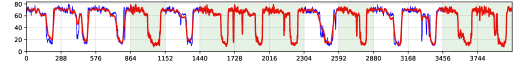
(a) Sensor #2.

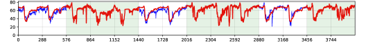
(b) Sensor #3.

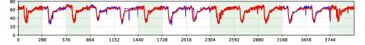
(c) Sensor #4.

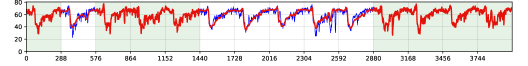
(d) Sensor #5.

Figure 2: Imputation of LATC-TNN on the PeMS data (first two weeks). We show the results from four sensors under 40% NM pattern. The green panels indicate partially observed input data, the blue curves show the ground truth values, and the red curves show the recovered data.

(a) Location #1.

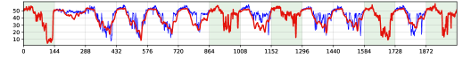
(b) Location #2.

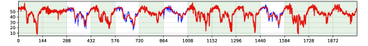
(c) Location #3.

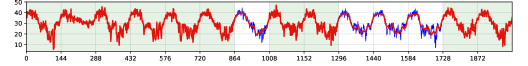
(d) Location #4.

Figure 3: Imputation of LATC-TNN on the Guangzhou data (first two weeks). We show the results from four locations under 40% NM pattern. The green panels indicate partially observed input data, the blue curves show the ground truth values, and the red curves show the recovered data.

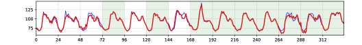
(a) Client #2.

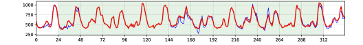
(b) Client #4.

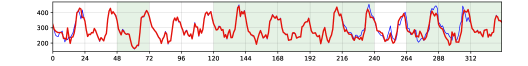
(c) Client #5.

Figure 4: Imputation of LATC-TNN on the Electricity data (first two weeks). We show the results from three clients under 40% NM pattern. The green panels indicate partially observed input data, the blue curves show the ground truth values, and the red curves show the recovered data.

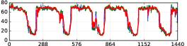
(a) Sensor #2 (40%, RM).

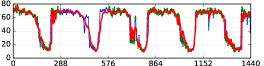
(b) Sensor #2 (40%, NM).

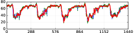
(c) Sensor #3 (40%, RM).

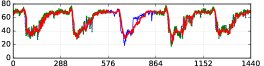
(d) Sensor #3 (40%, NM).

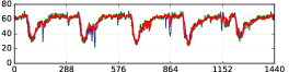
(e) Sensor #4 (40%, RM).

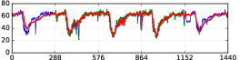
(f) Sensor #4 (40%, NM).

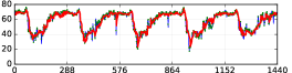
(g) Sensor #5 (40%, RM).

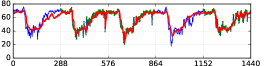
(h) Sensor #5 (40%, NM).

Figure 5: Rolling prediction of LATC-TNN on the PeMS data ($\tau=9$ and $S=160$, 1440 time points in total). We show the results from four sensors under different missing scenarios. The green dots represent partially observed input data, the blue curves show the ground truth values, and the red curves show the prediction.

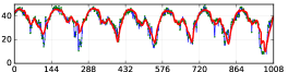
(a) Location #1 (40%, RM).

(b) Location #1 (40%, NM).

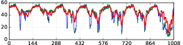
(c) Location #2 (40%, RM).

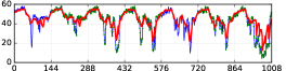
(d) Location #2 (40%, NM).

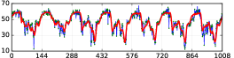
(e) Location #3 (40%, RM).

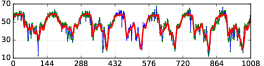
(f) Location #3 (40%, NM).

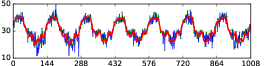
(g) Location #4 (40%, RM).

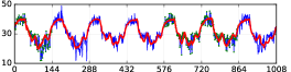
(h) Location #4 (40%, NM).

Figure 6: Rolling prediction of LATC-TNN on the Guangzhou data ($\tau=12$ and $S=84$, 1008 time points in total). We show the results from four locations under different missing scenarios. The green dots represent partially observed input data, the blue curves show the ground truth values, and the red curves show the prediction.

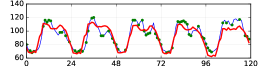
(a) Client #2 (40%, RM).

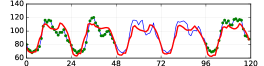
(b) Client #2 (40%, NM).

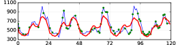
(c) Client #4 (40%, RM).

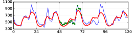
(d) Client #4 (40%, NM).

(e) Client #5 (40%, RM).

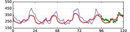
(f) Client #5 (40%, NM).

Figure 7: Rolling prediction of LATC-TNN on the Electricity data ($\tau=6$ and $S=20$, 120 time points in total). We show the results from three clients under different missing scenarios. The green dots represent partially observed input data, the blue curves show the ground truth values, and the red curves show the prediction.

Appendix C Derivation detail

In this section, we provide detailed derivation of some optimization problems in LATC.

C.1 Updating the variable $\boldsymbol{\mathcal{X}}_{k},k=1,2,3$

For the optimization problem in Eq. (7), we can first write it as follows,

$$\boldsymbol{\mathcal{X}}_{k}^{l+1}:= \operatorname{arg}\min_{\boldsymbol{\mathcal{X}}}~{}\alpha_{k}\|\boldsymbol{\mathcal{X}}_{(k)}\|_{*}+\frac{\rho}{2}\|\mathcal{Q}^{-1}(\boldsymbol{\mathcal{X}})-\boldsymbol{Z}^{l}\|_{F}^{2}+\big{\langle}\mathcal{Q}^{-1}(\boldsymbol{\mathcal{X}})-\boldsymbol{Z}^{l},\mathcal{Q}^{-1}(\boldsymbol{\mathcal{T}}_{k}^{l})\big{\rangle},$$ (19)

$$= \operatorname{arg}\min_{\boldsymbol{\mathcal{X}}}~{}\alpha_{k}\|\boldsymbol{\mathcal{X}}_{(k)}\|_{*}+\frac{\rho}{2}\big{\langle}\mathcal{Q}^{-1}(\boldsymbol{\mathcal{X}})-\boldsymbol{Z}^{l},\mathcal{Q}^{-1}(\boldsymbol{\mathcal{X}})-\boldsymbol{Z}^{l}\big{\rangle}+\big{\langle}\mathcal{Q}^{-1}(\boldsymbol{\mathcal{X}}),\mathcal{Q}^{-1}(\boldsymbol{\mathcal{T}}_{k}^{l})\big{\rangle}$$

$$= \operatorname{arg}\min_{\boldsymbol{\mathcal{X}}}~{}\alpha_{k}\|\boldsymbol{\mathcal{X}}_{(k)}\|_{*}+\frac{\rho}{2}\big{\langle}\mathcal{Q}^{-1}(\boldsymbol{\mathcal{X}}),\mathcal{Q}^{-1}(\boldsymbol{\mathcal{X}})\big{\rangle}-\big{\langle}\mathcal{Q}^{-1}(\boldsymbol{\mathcal{X}}),\rho\boldsymbol{Z}^{l}-\mathcal{Q}^{-1}(\boldsymbol{\mathcal{T}}_{k}^{l})\big{\rangle}$$

$$= \operatorname{arg}\min_{\boldsymbol{\mathcal{X}}}~{}\alpha_{k}\|\boldsymbol{\mathcal{X}}_{(k)}\|_{*}+\frac{\rho}{2}\big{\langle}\mathcal{Q}^{-1}(\boldsymbol{\mathcal{X}})-\boldsymbol{Z}^{l}+\frac{1}{\rho}\mathcal{Q}^{-1}(\boldsymbol{\mathcal{T}}_{k}^{l}),\mathcal{Q}^{-1}(\boldsymbol{\mathcal{X}})-\boldsymbol{Z}^{l}+\frac{1}{\rho}\mathcal{Q}^{-1}(\boldsymbol{\mathcal{T}}_{k}^{l})\big{\rangle}$$

$$= \operatorname{arg}\min_{\boldsymbol{\mathcal{X}}}~{}\alpha_{k}\|\boldsymbol{\mathcal{X}}_{(k)}\|_{*}+\frac{\rho}{2}\|\mathcal{Q}^{-1}(\boldsymbol{\mathcal{X}})-\boldsymbol{Z}^{l}+\mathcal{Q}^{-1}(\boldsymbol{\mathcal{T}}_{k}^{l})/\rho\|_{F}^{2}$$

$$= \operatorname{arg}\min_{\boldsymbol{\mathcal{X}}}~{}\alpha_{k}\|\boldsymbol{\mathcal{X}}_{(k)}\|_{*}+\frac{\rho}{2}\|\boldsymbol{\mathcal{X}}_{(k)}-\mathcal{Q}(\boldsymbol{Z}^{l})_{(k)}+\boldsymbol{\mathcal{T}}_{k(k)}^{l}/\rho\|_{F}^{2},$$

then applying Lemma 3, we can therefore obtain the optimal solution to the variable $\boldsymbol{\mathcal{X}}$ as

$$\boldsymbol{\mathcal{X}}_{k}^{l+1}:=\operatorname{fold}_{k}\left(\mathcal{D}_{\alpha_{k}/\rho}(\mathcal{Q}(\boldsymbol{Z}^{l})_{(k)}-\boldsymbol{\mathcal{T}}_{k(k)}^{l}/\rho)\right).$$ (20)

Similarly, we can write the closed-form solution to Eq. (16) with TNN minimization.

C.2 Updating the variable $\boldsymbol{Z}$

For the optimization problem in Eq. (8), we have

$$\boldsymbol{Z}^{l+1}_{[:h_{d}]}:= \operatorname{arg}\min_{\boldsymbol{Z}}~{}\sum_{k}\left(\frac{\rho}{2}\|\mathcal{Q}^{-1}(\boldsymbol{\mathcal{X}}_{k}^{l+1})_{[:h_{d}]}-\boldsymbol{Z}\|_{F}^{2}+\big{\langle}\mathcal{Q}^{-1}(\boldsymbol{\mathcal{X}}_{k}^{l+1})_{[:h_{d}]}-\boldsymbol{Z},\mathcal{Q}^{-1}(\boldsymbol{\mathcal{T}}_{k}^{l})_{[:h_{d}]}\big{\rangle}\right)$$ (21)

$$= \operatorname{arg}\min_{\boldsymbol{Z}}~{}\sum_{k}\left(\frac{\rho}{2}\big{\langle}\boldsymbol{Z},\boldsymbol{Z}\big{\rangle}-\rho\big{\langle}\boldsymbol{Z},\mathcal{Q}^{-1}(\boldsymbol{\mathcal{X}}_{k}^{l+1}+\boldsymbol{\mathcal{T}}_{k}^{l}/\rho)_{[:h_{d}]}\big{\rangle}\right)$$

$$= \operatorname{arg}\min_{\boldsymbol{Z}}~{}\frac{\rho}{2}\sum_{k}\big{\langle}\boldsymbol{Z}-\mathcal{Q}^{-1}(\boldsymbol{\mathcal{X}}_{k}^{l+1}+\boldsymbol{\mathcal{T}}_{k}^{l}/\rho)_{[:h_{d}]},\boldsymbol{Z}-\mathcal{Q}^{-1}(\boldsymbol{\mathcal{X}}_{k}^{l+1}+\boldsymbol{\mathcal{T}}_{k}^{l}/\rho)_{[:h_{d}]}\big{\rangle}$$

$$= \frac{1}{3}\sum_{k}\mathcal{Q}^{-1}(\boldsymbol{\mathcal{X}}_{k}^{l+1}+\boldsymbol{\mathcal{T}}_{k}^{l}/\rho)_{[:h_{d}]}.$$

For the optimization problem in Eq. (9), we have

$$\boldsymbol{Z}^{l+1}_{[h_{d}+1:]} \begin{aligned} &:=\operatorname{arg}\min_{\boldsymbol{Z}}~{}\sum_{m}\frac{\lambda}{2}\|\boldsymbol{z}_{m,[h_{d}+1:]}-\boldsymbol{Q}_{m}\boldsymbol{a}_{m}\|_{2}^{2}+\\ &\sum_{k}\left(\frac{\rho}{2}\|\mathcal{Q}^{-1}(\boldsymbol{\mathcal{X}}_{k}^{l+1})_{[h_{d}+1:]}-\boldsymbol{Z}\|_{F}^{2}+\big{\langle}\mathcal{Q}^{-1}(\boldsymbol{\mathcal{X}}_{k}^{l+1})_{[h_{d}+1:]}-\boldsymbol{Z},\mathcal{Q}^{-1}(\boldsymbol{\mathcal{T}}_{k}^{l})_{[h_{d}+1:]}\big{\rangle}\right)\\ \end{aligned}$$ (22)

$$\Rightarrow\boldsymbol{z}_{m,[h_{d}+1:]}:= \operatorname{arg}\min_{\boldsymbol{z}}~{}\frac{\lambda}{2}\|\boldsymbol{z}-\boldsymbol{Q}_{m}\boldsymbol{a}_{m}\|_{F}^{2}+\frac{\rho}{2}\|\boldsymbol{z}-\frac{1}{3}\sum_{k}\mathcal{Q}^{-1}(\boldsymbol{\mathcal{X}}_{k}^{l+1}+\boldsymbol{\mathcal{T}}_{k}^{l}/\rho)_{m,[h_{d}+1:]}\|_{F}^{2}$$ (23)

$$= \frac{\lambda}{\rho+\lambda}\boldsymbol{Q}_{m}\boldsymbol{a}_{m}^{l}+\frac{1}{3(\rho+\lambda)}\sum_{k}\mathcal{Q}^{-1}(\rho\boldsymbol{\mathcal{X}}_{k}^{l+1}+\boldsymbol{\mathcal{T}}_{k}^{l})_{m,[h_{d}+1:]}.$$

References

- [1] R. J. Hyndman and G. Athanasopoulos, Forecasting: Principles and Practice, 2nd ed. OTexts, 2018.
- [2] C. Faloutsos, J. Gasthaus, T. Januschowski, and Y. Wang, “Forecasting big time series: old and new,” Proceedings of the VLDB Endowment, vol. 11, no. 12, pp. 2102–2105, 2018.
- [3] L. Xiong, X. Chen, T.-K. Huang, J. Schneider, and J. G. Carbonell, “Temporal collaborative filtering with bayesian probabilistic tensor factorization,” in Proceedings of the 2010 SIAM International Conference on Data Mining, 2010, pp. 211–222.
- [4] P. Jing, Y. Su, X. Jin, and C. Zhang, “High-order temporal correlation model learning for time-series prediction,” IEEE Transactions on Cybernetics, vol. 49, no. 6, pp. 2385–2397, 2018.
- [5] H.-F. Yu, N. Rao, and I. S. Dhillon, “Temporal regularized matrix factorization for high-dimensional time series prediction,” in Advances in Neural Information Processing Systems, 2016, pp. 847–855.
- [6] M. T. Bahadori, Q. R. Yu, and Y. Liu, “Fast multivariate spatio-temporal analysis via low rank tensor learning,” in Advances in Neural Information Processing Systems, 2014, pp. 3491–3499.
- [7] L. Li, X. Su, Y. Zhang, Y. Lin, and Z. Li, “Trend modeling for traffic time series analysis: An integrated study,” IEEE Transactions on Intelligent Transportation Systems, vol. 16, no. 6, pp. 3430–3439, 2015.
- [8] R. Yu, S. Zheng, A. Anandkumar, and Y. Yue, “Long-term forecasting using tensor-train RNNs,” Arxiv, 2017.
- [9] G. Lai, W.-C. Chang, Y. Yang, and H. Liu, “Modeling long-and short-term temporal patterns with deep neural networks,” in ACM SIGIR Conference on Research & Development in Information Retrieval, 2018, pp. 95–104.
- [10] S. Li, X. Jin, Y. Xuan, X. Zhou, W. Chen, Y.-X. Wang, and X. Yan, “Enhancing the locality and breaking the memory bottleneck of transformer on time series forecasting,” in Advances in Neural Information Processing Systems, 2019, pp. 5244–5254.
- [11] R. Sen, H.-F. Yu, and I. S. Dhillon, “Think globally, act locally: A deep neural network approach to high-dimensional time series forecasting,” in Advances in Neural Information Processing Systems, 2019, pp. 4838–4847.
- [12] M. R. de Araujo, P. M. P. Ribeiro, and C. Faloutsos, “Tensorcast: Forecasting with context using coupled tensors,” in IEEE International Conference on Data Mining (ICDM), 2017, pp. 71–80.
- [13] L. Sun and X. Chen, “Bayesian temporal factorization for multidimensional time series prediction,” arXiv preprint arXiv:1910.06366, 2019.
- [14] S. Roberts, M. Osborne, M. Ebden, S. Reece, N. Gibson, and S. Aigrain, “Gaussian processes for time-series modelling,” Philosophical Transactions of the Royal Society A: Mathematical, Physical and Engineering Sciences, vol. 371, p. 20110550, 2013.
- [15] N. Golyandina, V. Nekrutkin, and A. A. Zhigljavsky, Analysis of Time Series Structure: SSA and Related Techniques. CRC press, 2001.
- [16] I. Markovsky, Low Rank Approximation Algorithms, Implementation, Applications, 2nd ed. Springer, 2019.
- [17] Y. Chen and Y. Chi, “Robust spectral compressed sensing via structured matrix completion,” IEEE Transactions on Information Theory, vol. 60, no. 10, pp. 6576–6601, 2014.
- [18] J. Gillard and K. Usevich, “Structured low-rank matrix completion for forecasting in time series analysis,” International Journal of Forecasting, vol. 34, no. 4, pp. 582–597, 2018.
- [19] A. Agarwal, M. J. Amjad, D. Shah, and D. Shen, “Model agnostic time series analysis via matrix estimation,” Proceedings of the ACM on Measurement and Analysis of Computing Systems, vol. 2, no. 3, pp. 1–39, 2018.
- [20] T. Yokota, B. Erem, S. Guler, S. K. Warfield, and H. Hontani, “Missing slice recovery for tensors using a low-rank model in embedded space,” in IEEE Conference on Computer Vision and Pattern Recognition, 2018, pp. 8251–8259.
- [21] S. Zhang and M. Wang, “Correction of corrupted columns through fast robust hankel matrix completion,” IEEE Transactions on Signal Processing, vol. 67, no. 10, pp. 2580–2594, 2019.
- [22] Q. Shi, J. Yin, J. Cai, A. Cichocki, T. Yokota, L. Chen, M. Yuan, and J. Zeng, “Block Hankel tensor ARIMA for multiple short time series forecasting,” arXiv preprint arXiv:2002.12135, 2020.
- [23] M. Figueiredo, B. Ribeiro, and A. de Almeida, “Electrical signal source separation via nonnegative tensor factorization using on site measurements in a smart home,” IEEE Transactions on Instrumentation and Measurement, vol. 63, no. 2, pp. 364–373, 2013.
- [24] H. Tan, Y. Wu, B. Shen, P. J. Jin, and B. Ran, “Short-term traffic prediction based on dynamic tensor completion,” IEEE Transactions on Intelligent Transportation Systems, vol. 17, no. 8, pp. 2123–2133, 2016.
- [25] Z. Li, N. D. Sergin, H. Yan, C. Zhang, and F. Tsung, “Tensor completion for weakly-dependent data on graph for metro passenger flow prediction,” arXiv preprint arXiv:1912.05693, 2019.
- [26] X. Chen, J. Yang, and L. Sun, “A nonconvex low-rank tensor completion model for spatiotemporal traffic data imputation,” Transportation Research Part C: Emerging Technologies, 2020.
- [27] T. G. Kolda and B. W. Bader, “Tensor decompositions and applications,” SIAM Review, vol. 51, no. 3, pp. 455–500, 2009.
- [28] B. Recht, M. Fazel, and P. A. Parrilo, “Guaranteed minimum-rank solutions of linear matrix equations via nuclear norm minimization,” SIAM Review, vol. 52, no. 3, pp. 471–501, 2010.
- [29] J. Liu, P. Musialski, P. Wonka, and J. Ye, “Tensor completion for estimating missing values in visual data,” IEEE Transactions on Pattern Analysis and Machine Intelligence, vol. 35, no. 1, pp. 208–220, 2013.
- [30] J.-F. Cai, E. J. Candès, and Z. Shen, “A singular value thresholding algorithm for matrix completion,” SIAM Journal on Optimization, vol. 20, no. 4, pp. 1956–1982, 2010.
- [31] Y. Hu, D. Zhang, J. Ye, X. Li, and X. He, “Fast and accurate matrix completion via truncated nuclear norm regularization,” IEEE Transactions on Pattern Analysis and Machine Intelligence, vol. 35, no. 9, pp. 2117–2130, Sep. 2013.
- [32] Y. Zhang and Z. Lu, “Penalty decomposition methods for rank minimization,” in Advances in Neural Information Processing Systems, 2011, pp. 46–54.
- [33] K. Chen, H. Dong, and K.-S. Chan, “Reduced rank regression via adaptive nuclear norm penalization,” Biometrika, vol. 100, no. 4, pp. 901–920, 2013.
- [34] C. Lu, C. Zhu, C. Xu, S. Yan, and Z. Lin, “Generalized singular value thresholding,” in AAAI Conference on Artificial Intelligence (AAAI), 2015.