Median Matrix Completion: from Embarrassment to Optimality

Abstract

In this paper, we consider matrix completion with absolute deviation loss and obtain an estimator of the median matrix. Despite several appealing properties of median, the non-smooth absolute deviation loss leads to computational challenge for large-scale data sets which are increasingly common among matrix completion problems. A simple solution to large-scale problems is parallel computing. However, embarrassingly parallel fashion often leads to inefficient estimators. Based on the idea of pseudo data, we propose a novel refinement step, which turns such inefficient estimators into a rate (near-)optimal matrix completion procedure. The refined estimator is an approximation of a regularized least median estimator, and therefore not an ordinary regularized empirical risk estimator. This leads to a non-standard analysis of asymptotic behaviors. Empirical results are also provided to confirm the effectiveness of the proposed method.

1 Introduction

Matrix completion (MC) has recently gained a substantial amount of popularity among researchers and practitioners due to its wide applications; as well as various related theoretical advances Candès and Recht (2009); Candès and Plan (2010); Koltchinskii et al. (2011); Klopp (2014). Perhaps the most well-known example of a MC problem is the Netflix prize problem (Bennett and Lanning, 2007), of which the goal is to predict missing entries of a partially observed matrix of movie ratings. Two commonly shared challenges among MC problems are high dimensionality of the matrix and a huge proportion of missing entries. For instance, Netflix data has less than 1% of observed entries of a matrix with around $5\times 10^{5}$ rows and $2\times 10^{4}$ customers. With technological advances in data collection, we are confronting increasingly large matrices nowadays.

Without any structural assumption on the target matrix, it is well-known that MC is an ill-posed problem. A popular and often well-justified assumption is low rankness, which however leads to a challenging and non-convex rank minimization problem Srebro et al. (2005). The seminal works of Candès and Recht (2009); Candès and Tao (2010); Gross (2011) showed that, when the entries are observed without noise, a perfect recovery of a low-rank matrix can be achieved by a convex optimization via near minimal order of sample size, with high probability. As for the noisy setting, some earlier work (Candès and Plan, 2010; Keshavan et al., 2010; Chen, Chi, Fan, Ma and Yan, 2019) focused on arbitrary, not necessarily random, noise. In general, the arbitrariness may prevent asymptotic recovery even in a probability sense.

Recently, a significant number of works (e.g. Bach, 2008; Koltchinskii et al., 2011; Negahban and Wainwright, 2011; Rohde and Tsybakov, 2011; Negahban and Wainwright, 2012; Klopp, 2014; Cai and Zhou, 2016; Fan et al., 2019; Xia and Yuan, 2019) targeted at more amenable random error models, under which (near-)optimal estimators had been proposed. Among these work, trace regression model is one of the most popular models due to its regression formulation. Assume $N$ independent pairs $({\mathbf{X}}_{k},Y_{k})$, for $k=1,\dots,N$, are observed, where ${\mathbf{X}}_{k}$’s are random design matrices of dimension $n_{1}\times n_{2}$ and $Y_{k}$’s are response variables in $\mathbb{R}$. The trace regression model assumes

$$Y_{k}={\rm tr}\left({\mathbf{X}}_{k}^{\rm T}{\mathbf{A}}_{\star}\right)+\epsilon_{k},\qquad k=1,\dots,N,$$ (1.1)

where ${\rm tr}({\mathbf{A}})$ denotes the trace of a matrix ${\mathbf{A}}$, and ${\mathbf{A}}_{\star}\in\mathbb{R}^{n_{1}\times n_{2}}$ is an unknown target matrix. Moreover, the elements of $\bm{\epsilon}=(\epsilon_{1},\dots,\epsilon_{N})$ are $N$ i.i.d. random noise variables independent of the design matrices. In MC setup, the design matrices $\bm{X}_{k}$’s are assumed to lie in the set of canonical bases

$$\mathcal{X}=\{\bm{e}_{j}(n_{1})\bm{e}_{k}(n_{2})^{\rm T}:j=1,\dots,n_{1};k=1,\dots,n_{2}\},$$ (1.2)

where $\bm{e}_{j}(n_{1})$ is the $j$-th unit vector in $\mathbb{R}^{n_{1}}$, and $\bm{e}_{k}(n_{2})$ is the $k$-th unit vector in $\mathbb{R}^{n_{2}}$. Most methods then apply a regularized empirical risk minimization (ERM) framework with a quadratic loss. It is well-known that the quadratic loss is most suitable for light-tailed (sub-Gaussian) error, and leads to non-robust estimations. In the era of big data, a thorough and accurate data cleaning step, as part of data preprocessing, becomes virtually impossible. In this regard, one could argue that robust estimations are more desirable, due to their reliable performances even in the presence of outliers and violations of model assumptions. While robust statistics is a well-studied area with a rich history (Davies, 1993; Huber, 2011), many robust methods were developed for small data by today’s standards, and are deemed too computationally intensive for big data or complex models. This work can be treated as part of the general effort to broaden the applicability of robust methods to modern data problems.

1.1 Related Work

Many existing robust MC methods adopt regularized ERM and assume observations are obtained from a low-rank-plus-sparse structure $\bm{A}_{\star}+\bm{S}+\bm{E}$, where the low-rank matrix $\bm{A}_{\star}$ is the target uncontaminated component; the sparse matrix $\bm{S}$ models the gross corruptions (outliers) locating at a small proportion of entries; and $\bm{E}$ is an optional (dense) noise component. As gross corruptions are already taken into account, many methods with low-rank-plus-sparse structure are based on quadratic loss. Chandrasekaran et al. (2011); Candès et al. (2011); Chen et al. (2013); Li (2013) considered the noiseless setting (i.e., no $\bm{E}$) with an element-wisely sparse $\bm{S}$. Chen et al. (2011) studied the noiseless model with column-wisely sparse $\bm{S}$. Under the model with element-wisely sparse $\bm{S}$, Wong and Lee (2017) looked into the setting of arbitrary (not necessarily random) noise $\bm{E}$, while Klopp et al. (2017) and Chen et al. (2020) studied random (sub-Gaussian) noise model for $\bm{E}$. In particular, it was shown in Proposition 3 of Wong and Lee (2017) that in the regularized ERM framework, a quadratic loss with element-wise $\ell_{1}$ penalty on the sparse component is equivalent to a direct application of a Huber loss without the sparse component. Roughly speaking, this class of robust methods, based on the low-rank-plus-sparse structure, can be understood as regularized ERMs with Huber loss.

Another class of robust MC methods is based on the absolute deviation loss, formally defined in (2.1). The minimizer of the corresponding risk has an interpretation of median (see Section 2.1), and so the regularized ERM framework that applies absolute deviation loss is coined as median matrix completion (Elsener and van de Geer, 2018; Alquier et al., 2019). In the trace regression model, if the medians of the noise variables are zero, the median MC estimator can be treated as a robust estimation of $\bm{A}_{\star}$. Although median is one of the most commonly used robust statistics, the median MC methods have not been studied until recently. Elsener and van de Geer (2018) derived the asymptotic behavior of the trace-norm regularized estimators under both the absolute deviation loss and the Huber loss. Their convergence rates match with the rate obtained in Koltchinskii et al. (2011) under certain conditions. More complete asymptotic results have been developed in Alquier et al. (2019), which derives the minimax rates of convergence with any Lipschitz loss functions including absolute deviation loss.

To the best of our knowledge, the only existing computational algorithm of median MC in the literature is proposed by Alquier et al. (2019), which is an alternating direction method of multiplier (ADMM) algorithm developed for the quantile MC with median MC being a special case. However, this algorithm is slow and not scalable to large matrices due to the non-smooth nature of both the absolute deviation loss and the regularization term.

Despite the computational challenges, the absolute deviation loss has a few appealing properties as compared to the Huber loss. First, absolute deviation loss is tuning-free while Huber loss has a tuning parameter, which is equivalent to the tuning parameter in the entry-wise $\ell_{1}$ penalty in the low-rank-plus-sparse model. Second, absolute deviation loss is generally more robust than Huber loss. Third, the minimizer of expected absolute deviation loss is naturally tied to median, and is generally more interpretable than the minimizer of expected Huber loss (which may vary with its tuning parameter).

1.2 Our Goal and Contributions

Our goal is to develop a robust and scalable estimator for median MC, in large-scale problems. The proposed estimator approximately solves the regularized ERM with the non-differentiable absolute deviation loss. It is obtained through two major stages — (1) a fast and simple initial estimation via embarrassingly parallel computing and (2) a refinement stage based on pseudo data. As pointed out earlier (with more details in Section 2.2), existing computational strategy (Alquier et al., 2019) does not scale well with the dimensions of the matrix. Inspired by Mackey et al. (2015), a simple strategy is to divide the target matrix into small sub-matrices and perform median MC on every sub-matrices in an embarrassingly parallel fashion, and then naively concatenate all estimates of these sub-matrices to form an initial estimate of the target matrix. Therefore, most computations are done on much smaller sub-matrices, and hence this computational strategy is much more scalable. However, since low-rankness is generally a global (whole-matrix) structure, the lack of communications between the computations of different sub-matrices lead to sub-optimal estimation (Mackey et al., 2015). The key innovation of this paper is a fast refinement stage, which transforms the regularized ERM with absolute deviation loss into a regularized ERM with quadratic loss, for which many fast algorithms exist, via the idea of pseudo data. Motivated by Chen, Liu, Mao and Yang (2019), we develop the pseudo data based on a Newton-Raphson iteration in expectation. The construction of the pseudo data requires only a rough initial estimate (see Condition (C6) in Section 3), which is obtained in the first stage. As compared to Huber-loss-based methods (sparse-plus-low-rank model), the underlying absolute deviation loss is non-differentiable, leading to computational difficulty for large-scale problems. The proposed strategy involves a novel refinement stage to efficiently combine and improve the embarrassingly parallel sub-matrix estimations.

We are able to theoretically show that this refinement stage can improve the convergence rate of the sub-optimal initial estimator to near-optimal order, as good as the computationally expensive median MC estimator of Alquier et al. (2019). To the best of our knowledge, this theoretical guarantee for distributed computing is the first of its kind in the literature of matrix completion.

2 Model and Algorithms

2.1 Regularized Least Absolute Deviation Estimator

Let ${\mathbf{A}}_{\star}=(A_{\star,ij})_{i,j=1}^{n_{1},n_{2}}\in\mathbb{R}^{n_{1}\times n_{2}}$ be an unknown high-dimensional matrix. Assume the $N$ pairs of observations $\{({\mathbf{X}}_{k},Y_{k})\}_{k=1}^{N}$ satisfy the trace regression model (1.1) with noise $\{\varepsilon_{k}\}_{k=1}^{N}$. The design matrices are assumed to be i.i.d. random matrices that take values in $\mathcal{X}$ (1.2). Let $\pi_{st}=\Pr({\mathbf{X}}_{k}={\mathbf{e}}_{s}(n_{1}){\mathbf{e}}_{t}^{\rm T}(n_{2}))$ be the probability of observing (a noisy realization of) the $(s,t)$-th entry of ${\mathbf{A}}_{\star}$ and denote $\bm{\Pi}=(\pi_{1,1},\dots,\pi_{n_{1},n_{2}})^{\rm T}$. Instead of the uniform sampling where $\pi_{st}\equiv\pi$ (Koltchinskii et al., 2011; Rohde and Tsybakov, 2011; Elsener and van de Geer, 2018), out setup allows sampling probabilities to be different across entries, such as in Klopp (2014); Lafond (2015); Cai and Zhou (2016); Alquier et al. (2019). See Condition (C1) for more details. Overall, $(Y_{1},{\mathbf{X}}_{1},\varepsilon_{1}),\dots,(Y_{N},{\mathbf{X}}_{N},\varepsilon_{N})$ are i.i.d. tuples of random variables. For notation’s simplicity, we let $(Y,{\mathbf{X}},\varepsilon)$ be a generic independent tuple of random variables that have the same distribution as $(Y_{1},{\mathbf{X}}_{1},\varepsilon_{1})$. Without additional specification, the noise variable $\varepsilon$ is not identifiable. For example, one can subtract a constant from all entries of ${\mathbf{A}}_{\star}$ and add this constant to the noise. To identify the noise, we assume $\mathbb{P}(\epsilon\leq 0)=0.5$, which naturally leads to an interpretation of ${\mathbf{A}}_{\star}$ as median, i.e., $A_{\star,ij}$ is the median of $Y\mid{\mathbf{X}}={\mathbf{e}}_{i}(n_{1}){\mathbf{e}}_{j}(n_{2})^{\rm T}$. If the noise distribution is symmetric and light-tailed (so that the expectation exists), then $\mathbb{E}(\varepsilon_{k})=0$, and ${\mathbf{A}}_{\star}$ is the also the mean matrix ($A_{\star,ij}=\mathbb{E}(Y\mid{\mathbf{X}}={\mathbf{e}}_{i}(n_{1}){\mathbf{e}}_{j}(n_{2})^{\rm T})$), which aligns with the target of common MC techniques (Elsener and van de Geer, 2018). Let $f$ be the probability density function of the noise. For the proposed method, the required condition of $f$ is specified in Condition (C3) of Section 3, which is fairly mild and is satisfied by many heavy-tailed distributions whose expectation may not exist.

Define a hypothesis class $\mathcal{B}(a,n,m)=\{{\mathbf{A}}\in\mathbb{R}^{n\times m}:\|{\mathbf{A}}\|_{\infty}\leq a\}$ where $a>0$ such that ${\mathbf{A}}_{\star}\in\mathcal{B}(a,n,m)$. In this paper, we use the absolute deviation loss instead of the common quadratic loss (e.g., Candès and Plan, 2010; Koltchinskii et al., 2011; Klopp, 2014). According to Section 4 of the Supplementary Material (Elsener and van de Geer, 2018), ${\mathbf{A}}_{\star}$ is also characterized as the minimizer of the population risk:

$${\mathbf{A}}_{\star}=\underset{{\mathbf{A}}\in\mathcal{B}(a,n_{1},n_{2})}{\arg\min}\mathbb{E}\left\{\left|Y-{\rm tr}({\mathbf{X}}^{\rm T}{\mathbf{A}})\right|\right\}.$$ (2.1)

To encourage a low-rank solution, one natural candidate is the following regularized empirical risk estimator (Elsener and van de Geer, 2018; Alquier et al., 2019):

$$\widehat{\mathbf{A}}_{\text{LADMC}}=\underset{{\mathbf{A}}\in\mathcal{B}(a,n_{1},n_{2})}{\arg\min} \frac{1}{N}\sum_{k=1}^{N}\left|Y_{k}-{\rm tr}({\mathbf{X}}_{k}^{\rm T}{\mathbf{A}})\right|$$

$$+\lambda_{N}^{\prime}\left\|{\mathbf{A}}\right\|_{\ast},$$ (2.2)

where $\|{\mathbf{A}}\|_{\ast}$ denotes the nuclear norm and $\lambda_{N}^{\prime}\geq 0$ is a tuning parameter. The nuclear norm is a convex relaxation of the rank which flavors the optimization and analysis of the statistical property (Candès and Recht, 2009).

Due to non-differentiability of the absolute deviation loss, the objective function in (2.1) is the sum of two non-differentiable terms, rendering common computational strategies based on proximal gradient method (e.g., Mazumder et al., 2010; Wong and Lee, 2017) inapplicable. To the best of our knowledge, there is only one existing computational algorithm for (2.1), which is based on a direct application of alternating direction method of multiplier (ADMM) (Alquier et al., 2019). However, this algorithm is slow and not scalable in practice, when the sample size and the matrix dimensions are large, possibly due to the non-differentiable nature of the loss.

We aim to derive a computationally efficient method for estimating the median matrix ${\mathbf{A}}_{\star}$ in large-scale MC problems. More specifically, the proposed method consists of two stages: (1) an initial estimation via distributed computing (Section 2.2) and (2) a refinement stage to achieve near-optimal estimation (Section 2.3).

2.2 Distributed Initial Estimator

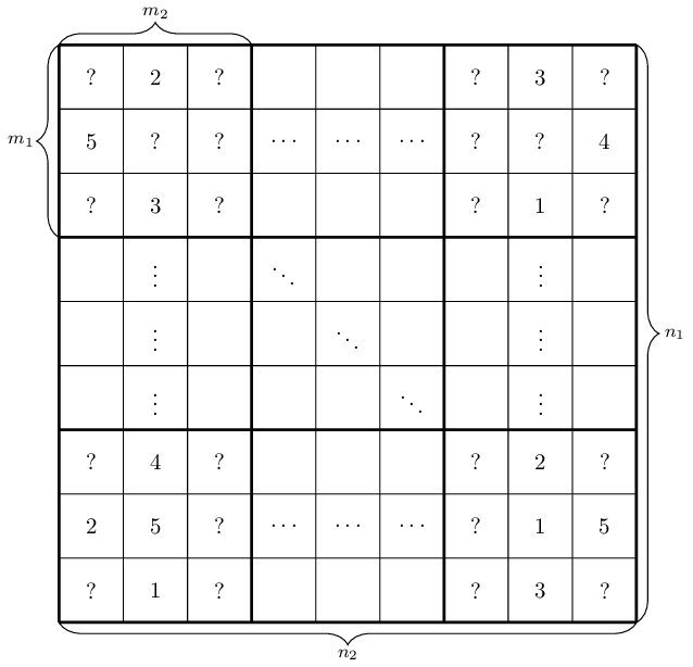
Figure 1: An example of dividing a matrix into sub-matrices.

Similar to many large-scale problems, it is common to harness distributed computing to overcome computational barriers. Motivated by Mackey et al. (2015), we divide the underlying matrix into several sub-matrices, estimate each sub-matrix separately in an embarrassingly parallel fashion and then combine them to form a computationally efficient (initial) estimator of ${\mathbf{A}}_{\star}$.

For the convenience of notations, suppose there exist integers $m_{1}$, $m_{2}$, $l_{1}$ and $l_{2}$ such that $l_{1}=n_{1}/m_{1}$ and $l_{2}=n_{2}/m_{2}$. (Otherwise, the following description can be easily extended with $l_{1}=\lfloor n_{1}/m_{1}\rfloor$ and $l_{2}=\lfloor n_{2}/m_{2}\rfloor$ which leads to slightly different sizes in several sub-matrices.) We divide the row indices $1,\dots,n_{1}$ into $l_{1}$ subsets evenly where each subset contains $m_{1}$ index and similarly divide the column indices $1,\dots,n_{2}$ into $l_{2}$ subsets evenly. Then we obtain $l_{1}l_{2}$ sub-matrices, denoted by ${\mathbf{A}}_{\star,l}\in\mathbb{R}^{m_{1}\times m_{2}}$ for $l=1,\dots,l_{1}l_{2}$. See Figure 1 for a pictorial illustration. Let $\bm{\Omega}_{l}$ be the index set of the observed entries within the $l$-th sub-matrix ${\mathbf{A}}_{\star,l}$, and $N_{l}$ be the corresponding number of observed entries. Next, we apply the ADMM algorithm of Alquier et al. (2019) to each sub-matrix ${\mathbf{A}}_{\star,l}$ and obtain corresponding median estimator:

$$\widehat{\mathbf{A}}_{\text{LADMC},l}=\underset{{\mathbf{A}}_{l}\in\mathcal{B}(a,m_{1},m_{2})}{\arg\min} \frac{1}{N_{l}}\sum_{k\in\bm{\Omega}_{l}}\left|Y_{k}-{\rm tr}({\mathbf{X}}_{l,k}^{\rm T}{\mathbf{A}}_{l})\right|$$

$$+\lambda_{N_{l},l}\left\|{\mathbf{A}}_{l}\right\|_{\ast},$$ (2.3)

where ${\mathbf{X}}_{l,k}$ is a corresponding sub-design matrix of dimensions $m_{1}\times m_{2}$ and $\lambda_{N_{l},l}\geq 0$ is a tuning parameter. Note that the most computationally intensive sub-routine in the ADMM algorithm of Alquier et al. (2019) is (repeated applications of) SVD. For sub-matrices of dimension $m_{1}\times m_{2}$, the computational complexity of a single SVD reduced from $\mathcal{O}(n_{1}^{2}n_{2}+n_{1}n_{2}^{2})$ to $\mathcal{O}(m_{1}^{2}m_{2}+m_{1}m_{2}^{2})$.

After we have all the $\widehat{\mathbf{A}}_{\text{LADMC},l}$ for $l=1,\dots,l_{1}l_{2}$, we can put these estimators of the sub-matrices back together according to their original positions in the target matrix (see Figure 1), and form an initial estimator $\widehat{\mathbf{A}}_{\text{LADMC},0}$.

This computational strategy is conceptually simple and easily implementable. However, despite the low-rank estimations for each sub-matrix, combining them directly cannot guarantee low-rankness of $\widehat{\mathbf{A}}_{\text{LADMC},0}$. Also, the convergence rate of $\widehat{\mathbf{A}}_{\text{LADMC},0}$ is not guaranteed to be (near-)optimal, as long as $m_{1},m_{2}$ are of smaller order than $n_{1},n_{2}$ respectively. See Theorem 1(i) in Section 3. However, for computational benefits, it is desirable to choose small $m_{1},m_{2}$. In the next section, we leverage this initial estimator and formulate a refinement stage.

2.3 The Idea of Refinement

The proposed refinement stage is based on a form of pseudo data, which leverages the idea from the Newton-Raphson iteration. To describe this idea, we start from the stochastic optimization problem (2.1). Write the loss function as $L({\mathbf{A}};\{Y,{\mathbf{X}}\})=|Y-{\rm tr}({\mathbf{X}}^{\rm T}{\mathbf{A}})|$. To solve this stochastic optimization problem, the population version of the Newton-Raphson iteration takes the following form

$$\text{vec}({\mathbf{A}}_{1})=\text{vec}(\widehat{\mathbf{A}}_{0})-{\mathbf{H}}(\widehat{\mathbf{A}}_{0})^{-1}\mathbb{E}_{(Y,{\mathbf{X}})}\left[\bm{l}(\widehat{\mathbf{A}}_{0};\{Y,{\mathbf{X}}\})\right],$$ (2.4)

where $(Y,{\mathbf{X}})$ is defined in Section 2.1 to be independent of the data; $\text{vec}({\mathbf{A}})$ is the vectorization of the matrix ${\mathbf{A}}$; $\widehat{\mathbf{A}}_{0}$ is an initial estimator (to be specified below); and $\bm{l}({\mathbf{A}};\{Y,{\mathbf{X}}\})$ is the sub-gradient of $L({\mathbf{A}};\{Y,{\mathbf{X}}\})$ with respect to $\text{vec}({\mathbf{A}})$. One can show that the population Hessian matrix takes the form ${\mathbf{H}}({\mathbf{A}})=2\mathbb{E}_{(Y,{\mathbf{X}})}(f\{{\rm tr}({\mathbf{X}}^{\rm T}({\mathbf{A}}-{\mathbf{A}}_{\star})\}){\rm diag}(\bm{\Pi})$, where we recall that $\bm{\Pi}=(\pi_{1,1},\dots,\pi_{n_{1},n_{2}})^{\rm T}$ is the vector of observation probabilities; and ${\rm diag}(\cdot)$ transforms a vector into a diagonal matrix whose diagonal is the vector. Also, it can be shown that $\mathbb{E}_{(Y,{\mathbf{X}})}[\bm{l}({\mathbf{A}};\{Y,{\mathbf{X}}\})]=\bm{\Pi}\mathbb{E}_{(Y,{\mathbf{X}})}\{2\mathds{I}\left[Y-{\rm tr}({\mathbf{X}}^{\rm T}{\mathbf{A}})\leq 0\right]-1\}$. Recall that $f(x)$ is the density function of the noise $\epsilon$.

By using ${\mathbf{H}}({\mathbf{A}}_{\star})=2f(0){\rm diag}(\bm{\Pi})$ in (2.4), we obtain the following approximation. When the initial estimator $\widehat{\mathbf{A}}_{0}$ is close to the minimizer ${\mathbf{A}}_{\star}$,

$$\text{vec}({\mathbf{A}}_{1})\approx\text{vec}(\widehat{\mathbf{A}}_{0})$$

$$\qquad-[2f(0){\rm diag}(\bm{\Pi})]^{-1}\mathbb{E}_{(Y,{\mathbf{X}})}[\bm{l}(\widehat{\mathbf{A}}_{0};\{Y,{\mathbf{X}}\})]$$

$$=\mathbb{E}_{(Y,{\mathbf{X}})}\left\{\text{vec}(\widehat{\mathbf{A}}_{0})\right.$$

$$\qquad-\left.[f(0)]^{-1}\left(\mathds{I}\left[Y\leq{\rm tr}({\mathbf{X}}^{\rm T}\widehat{\mathbf{A}}_{0})\right]-\frac{1}{2}\right)\mathds{1}_{n_{1}n_{2}}\right\}$$

$$=[{\rm diag}(\bm{\Pi})]^{-1}\mathbb{E}_{(Y,{\mathbf{X}})}\left[\text{vec}({\mathbf{X}})\left\{\text{vec}({\mathbf{X}})^{\rm T}\text{vec}(\widehat{\mathbf{A}}_{0})\right.\right.$$

$$\qquad\left.\left.-[f(0)]^{-1}\left(\mathds{I}\left[Y\leq{\rm tr}({\mathbf{X}}^{\rm T}\widehat{\mathbf{A}}_{0})\right]-\frac{1}{2}\right)\right\}\right]$$

$$=[{\rm diag}(\bm{\Pi})]^{-1}\mathbb{E}_{(Y,{\mathbf{X}})}\left(\mathrm{vec}({\mathbf{X}})\tilde{Y}^{o}\right)$$ (2.5)

$$=\{\mathbb{E}_{(Y,{\mathbf{X}})}[\text{vec}({\mathbf{X}})\text{vec}({\mathbf{X}})^{\rm T}]\}^{-1}\mathbb{E}_{(Y,{\mathbf{X}})}\left(\text{vec}({\mathbf{X}})\tilde{Y}^{0}\right)$$

where we define the theoretical pseudo data

$$\widetilde{Y}^{o}={\rm tr}({\mathbf{X}}^{\rm T}\widehat{\mathbf{A}}_{0})-[f(0)]^{-1}\left(\mathds{I}\left[Y\leq{\rm tr}({\mathbf{X}}^{\rm T}\widehat{\mathbf{A}}_{0})\right]-\frac{1}{2}\right).$$

Here $\mathds{1}_{n_{1}n_{2}}$ denotes the vector of dimension $n_{1}n_{2}$ with all elements equal to 1. Clearly, (2.3) is the vectorization of the solution to $\arg\min_{{\mathbf{A}}}\mathbb{E}_{(Y,{\mathbf{X}})}\{\widetilde{Y}^{o}-{\rm tr}({\mathbf{X}}^{\rm T}{\mathbf{A}})\}^{2}$, where ${\rm tr}({\mathbf{X}}^{\rm T}{\mathbf{A}})\}=\text{vec}({\mathbf{X}})^{\rm T}\text{vec}({\mathbf{A}})$. From this heuristic argument, we can approximate the population Newton update by a least square solution based on the pseudo data $\tilde{Y}^{0}$, when we start from an $\widehat{\mathbf{A}}_{0}$ close enough to ${\mathbf{A}}_{\star}$. Without the knowledge of $f(0)$, the pseudo data cannot be used. In the above, $f(0)$ can be easily estimated by the kernel density estimator:

$$\widehat{f}(0)=\frac{1}{Nh}\sum_{k=1}^{N}K\left(\frac{Y_{k}-{\rm tr}({\mathbf{X}}_{k}^{\rm T}\widehat{\mathbf{A}}_{0})}{h}\right),$$

where $K(x)$ is a kernel function which satisfies Condition (C4) and $h>0$ is the bandwidth. For each $1\leq k\leq N$, we define the actual pseudo data $\widetilde{\mathbf{Y}}$ used in our proposed procedure to be

$$\widetilde{Y}_{k}={\rm tr}({\mathbf{X}}_{k}^{\rm T}\widehat{\mathbf{A}}_{0})-[\widehat{f}(0)]^{-1}\left(\mathds{I}\left[Y_{k}\leq{\rm tr}({\mathbf{X}}_{k}^{\rm T}\widehat{\mathbf{A}}_{0})\right]-\frac{1}{2}\right),$$

and $\widetilde{\mathbf{Y}}=(\widetilde{Y}_{k})$. For finite sample, regularization is imposed to estimate the high-dimensional parameter ${\mathbf{A}}_{\star}$. By using $\widetilde{\mathbf{Y}}$, one natural candidate for the estimator of ${\mathbf{A}}_{\star}$ is given by

$$\widehat{\mathbf{A}}=\underset{{\mathbf{A}}\in\mathcal{B}(a,n_{1},n_{2})}{\arg\min} \frac{1}{N}\sum_{k=1}^{N}\left(\widetilde{Y}_{k}-{\rm tr}({\mathbf{X}}_{k}^{\rm T}{\mathbf{A}})\right)^{2}$$

$$+\lambda_{N}\left\|{\mathbf{A}}\right\|_{\ast},$$ (2.6)

where $\|\cdot\|_{\ast}$ is the nuclear norm and $\lambda_{N}\geq 0$ is the tuning parameter. If $\widetilde{\mathbf{Y}}$ is replaced by ${\mathbf{Y}}$, the optimization (2.3) is a common nuclear-norm regularized empirical risk estimator with quadratic loss which has been well studied in the literature (Candès and Recht, 2009; Candès and Plan, 2010; Koltchinskii et al., 2011; Klopp, 2014). Therefore, with the knowledge of $\widetilde{\mathbf{Y}}$, corresponding computational algorithms can be adopted to solve (2.3). Note that the pseudo data are based on an initial estimator $\widehat{\mathbf{A}}_{0}$. In Section 3, we show that any initial estimator that fulfills Condition (C5) can be improved by (2.3), which is therefore called a refinement step. It is easy to verify that the initial estimator $\widehat{\mathbf{A}}_{\text{LADMC},0}$ in Section 2.2 fulfills such condition. Note that the initial estimator, like $\widehat{\mathbf{A}}_{\text{LADMC},0}$, introduces complicated dependencies among the entries of $\widetilde{\mathbf{Y}}$, which brings new challenges in analyzing (2.3), as opposed to the common estimator based on ${\mathbf{Y}}$ with independent entries.

From our theory (Section 3), the refined estimator (2.3) improves upon the initial estimator. Depending on how bad the initial estimator is, a single refinement step may not be good enough to achieve a (near-)optimal estimator. But this can remedied by reapplying the refinement step again and again. In Section 3, we show that a finite number of application of the refinement step is enough. In our numerical experiments, 4–5 applications would usually produce enough improvement. Write $\widehat{\mathbf{A}}^{(1)}=\widehat{\mathbf{A}}$ given in (2.3) as the estimator from the first iteration and we can construct an iterative procedure to estimate ${\mathbf{A}}_{\star}$. In particular, let $\widehat{\mathbf{A}}^{(t-1)}$ be the estimator in the $(t-1)$-th iteration. Define

$$\widehat{f}^{(t)}(0)=\frac{1}{Nh_{t}}\sum_{k=1}^{N}K\left(\frac{Y_{k}-{\rm tr}({\mathbf{X}}_{k}^{\rm T}\widehat{\mathbf{A}}^{(t-1)})}{h_{t}}\right),$$

where $K(x)$ is the same smoothing function used to estimate $f(0)$ in the first step and $h_{t}\to 0$ is the bandwidth for the $t$-th iteration. Similarly, for each $1\leq k\leq N$, define

$$\widetilde{Y}_{k}^{(t)}= {\rm tr}({\mathbf{X}}_{k}^{\rm T}\widehat{\mathbf{A}}^{(t-1)})-\left(\widehat{f}^{(t)}\left(0\right)\right)^{-1}\times$$

$$\left(\mathds{I}\left[Y_{k}\leq{\rm tr}({\mathbf{X}}_{k}^{\rm T}\widehat{\mathbf{A}}^{(t-1)})\right]-\frac{1}{2}\right).$$ (2.7)

We propose the following estimator

$$\widehat{\mathbf{A}}^{(t)}=\underset{{\mathbf{A}}\in\mathcal{B}(a,n_{1},n_{2})}{\arg\min} \frac{1}{N}\sum_{k=1}^{N}\left(\widetilde{Y}_{k}^{(t)}-{\rm tr}({\mathbf{X}}_{k}^{\rm T}{\mathbf{A}})\right)^{2}$$

$$+\lambda_{N,t}\left\|{\mathbf{A}}\right\|_{\ast},$$ (2.8)

where $\lambda_{N,t}$ is the tunning parameter in the $t$-th iteration. To summarize, we list the full algorithm in Algorithm 1.

Algorithm 1 Distributed Least Absolute Deviation Matrix Completion

Input: Observed data pairs $\{{\mathbf{X}}_{k},Y_{k}\}$ for $k=1,\ldots,N$, number of observations $N$, dimensions of design matrix ${\mathbf{X}}$ $n_{1},n_{2}$, dimensions of sub-matrices to construct the initial estimator $m_{1},m_{2}$ and the split subsets $\bm{\Omega}_{l}$ for $l=1,\dots,l_{1}l_{2}$, kernel function $K$, a sequence of bandwidths $h_{t}$ and the regularization parameters $\lambda_{N,t}$ for $t=1,\dots,T$.

1:  Get the robust low-rank estimator of each ${\mathbf{A}}_{\star,l}$ by solving the minimization problem (2.2) in parallel.

2:  Set $\widehat{\mathbf{A}}^{(0)}$ to be the same as the initial estimator $\widehat{\mathbf{A}}_{\text{LADMC},0}$ by putting $\widehat{\mathbf{A}}_{\text{LADMC},l}$ together.

3:  for $t=1,2\ldots,T$ do

4:     Compute $\widehat{f}^{(t)}(0):=(Nh_{t})^{-1}\sum_{k=1}^{N}K(h_{t}^{-1}(Y_{k}-{\rm tr}\{{\mathbf{X}}_{k}^{\rm T}\widehat{\mathbf{A}}^{(t-1)}\}))$.

5:     Construct the pseudo data $\{\widetilde{Y}_{k}^{(t)}\}$ by equation (2.3).

6:     Plugin the pseudo data $\{\widetilde{Y}_{k}^{(t)}\}$ and compute the estimator $\widehat{\mathbf{A}}^{(t)}$ by solving the minimization problem (2.3).

7:  end for

Output: The final estimator $\widehat{\mathbf{A}}^{(T)}$.

3 Theoretical Guarantee

To begin with, we introduce several notations. Let $m_{+}=m_{1}+m_{2}$, $m_{\max}=\max\{m_{1},m_{2}\}$ and $m_{\min}=\min\{m_{1},m_{2}\}$. Similarly, write $n_{+}=n_{1}+n_{2}$, $n_{\max}=\max\{n_{1},n_{2}\}$ and $n_{\min}=\min\{n_{1},n_{2}\}$. For a given matrix ${\mathbf{A}}=(A_{ij})\in\mathbb{R}^{n_{1}\times n_{2}}$, denote $\sigma_{i}({\mathbf{A}})$ be the $i$-th largest singular value of matrix ${\mathbf{A}}$. Let $\|{\mathbf{A}}\|=\sigma_{1}({\mathbf{A}})$, $\|{\mathbf{A}}\|_{F}=\sqrt{\sum_{i=1}^{n_{1}}\sum_{j=1}^{n_{2}}A_{ij}^{2}}$ and $\|{\mathbf{A}}\|_{\ast}=\sum_{i=1}^{n_{\min}}\sigma_{i}({\mathbf{A}})$ be the spectral norm (operator norm), the infinity norm, the Frobenius norm and the trace norm of a matrix ${\mathbf{A}}$ respectively. Define a class of matrices $\mathcal{C}_{\ast}(n_{1},n_{2})=\{{\mathbf{A}}\in\mathbb{R}^{n_{1}\times n_{2}}:\|{\mathbf{A}}\|_{\ast}\leq 1\}$. Denote the rank of matrix ${\mathbf{A}}_{\star}$ by $r_{\star}=\text{rank}({\mathbf{A}}_{\star})$ for simplicity. With these notations, we describe the following conditions which are useful in our theoretical analysis.

(C1) For each $k=1,\dots,N$, the design matrix ${\mathbf{X}}_{k}$ takes value in the canonical basis $\mathcal{X}$ as defined in (1.2). There exist positive constants $\underline{c}$ and $\overline{c}$ such that for any $(s,t)\in\{1,\dots,n_{1}\}\times\{1,\dots,n_{2}\}$, $\underline{c}/(n_{1}n_{2})\leq\Pr({\mathbf{X}}_{k}={\mathbf{e}}_{s}(n_{1}){\mathbf{e}}_{t}^{\rm T}(n_{2}))\leq\overline{c}/(n_{1}n_{2})$.

(C2) The local dimensions $m_{1},m_{2}$ on each block satisfies $m_{1}\geq n_{1}^{c}$ and $m_{2}\geq n_{2}^{c}$ for some $0<c<1$. The number of observations in each block $N_{l}$ are comparable for all $l=1,\dots,l_{1}l_{2}$, i.e, $N_{l}\asymp m_{1}m_{2}N/(n_{1}n_{2})$.

(C3) The density function $f(\cdot)$ is Lipschitz continuous (i.e., $|f(x)-f(y)|\leq C_{L}|x-y|$ for any $x,y\in\mathbb{R}$ and some constant $C_{L}>0$). Moreover, there exists a constant $c>0$ such that $f(u)\geq c$ for any $|u|\leq 2a$. Also, $\Pr(\epsilon_{k}\leq 0)=0.5$ for each $k=1,\dots,N$.

Theorem 1 (Alquier et al. (2019), Theorem 4.6, Initial estimator).

Suppose that Conditions (C1)–(C3) hold and ${\mathbf{A}}_{\star}\in\mathcal{B}(a,n_{1},n_{2})$. For each $l=1,\dots,n_{1}n_{2}/(m_{1}m_{2})$, assume that there exists a matrix with rank at most $s_{l}$ in ${\mathbf{A}}_{\star,l}+(\rho_{s_{l}}/20)\mathcal{C}_{\ast}(m_{1},m_{2})$ where $\rho_{s_{l}}=C_{\rho}(s_{l}m_{1}m_{2})(\log(m_{+})/(m_{+}N_{l}))^{1/2}$ with the universal constant $C_{\rho}$.

(i) Then there exist universal constants $c(\underline{c},\overline{c})$ and $C$ such that with $\lambda_{N_{l},l}=c(\underline{c},\overline{c})\sqrt{\log(m_{+})/(m_{\min}N_{l})}$, the estimator $\widehat{\mathbf{A}}_{\text{LADMC},l}$ in (2.2) satisfies

$$\frac{1}{\sqrt{m_{1}m_{2}}}\left\|\widehat{\mathbf{A}}_{\text{LADMC},l}-{\mathbf{A}}_{\star,l}\right\|_{F}\leq C\min\left\{\sqrt{\frac{s_{l}m_{\max}\log(m_{+})}{N_{l}}},\left\|{\mathbf{A}}_{\star,l}\right\|_{\ast}^{1/2}\left(\frac{\log(m_{+})}{m_{\min}N_{l}}\right)^{1/4}\right\},$$ (3.1)

with probability at least $1-C\exp(-Cs_{l}m_{\max}\log(m_{+}))$.

(ii) Moreover, by putting these $l_{1}l_{2}$ estimators $\widehat{\mathbf{A}}_{\text{LADMC},l}$ together, for the same constant $C$ in (i), we have the initial estimator $\widehat{\mathbf{A}}_{\text{LADMC},0}$ satisfies

$$\frac{\left\|\widehat{\mathbf{A}}_{\text{LADMC},0}-{\mathbf{A}}_{\star}\right\|_{F}}{\sqrt{n_{1}n_{2}}}\leq C\min\left\{\sqrt{\frac{\{\sum_{l=1}^{l_{1}l_{2}}s_{l}\}m_{\max}\log(m_{+})}{N}},\right.$$

$$\left.\left(\sum_{l=1}^{l_{1}l_{2}}\left\|{\mathbf{A}}_{\star,l}\right\|_{\ast}^{1/2}\right)\left(\frac{m_{\max}\log(m_{+})}{n_{1}n_{2}N}\right)^{1/4}\right\},$$

with probability at least $1-C\exp(\log(n_{1}n_{2})-Cm_{\max}\log(m_{+}))$.

From Theorem 1, we can guarantee the convergence of the sub-matrix estimator $\widehat{\mathbf{A}}_{\text{LADMC},l}$ when $m_{1},m_{2}\to\infty$. For the initial estimator $\widehat{\mathbf{A}}_{\text{LADMC},0}$, under Condition (C3) and that all the sub-matrices are low-rank ($s_{l}\asymp 1$ for all $l$), we require the number of observation $N\geq C_{1}(m_{1}m_{2})^{-1}(n_{1}n_{2})m_{\max}\log(m_{+})$ for some constant $C_{1}$ to ensure the convergence. As for the rate of convergence, $\sqrt{(n_{1}n_{2})m_{\max}\log(m_{+})/(Nm_{1}m_{2})}$ is slower than the classical optimal rate $\sqrt{r_{\star}n_{\max}\log(n_{+})/N}$ when $m_{1},m_{2}$ are of smaller than $n_{1},n_{2}$ respectively.

(C4) Assume the kernel functions $K(\cdot)$ is integrable with $\int_{-\infty}^{\infty}K(u)du=1$. Moreover, assume that $K(\cdot)$ satisfies $K(u)=0$ if $|u|\geq 1$. Further, assume that $K(\cdot)$ is differentiable and its derivative $K^{\prime}(\cdot)$ is bounded.

(C5) The initial estimator $\widehat{\mathbf{A}}_{0}$ satisfies $(n_{1}n_{2})^{-1/2}\|\widehat{\mathbf{A}}_{0}-{\mathbf{A}}_{\star}\|_{F}=O_{\textsf{P}}((n_{1}n_{2})^{-1/2}a_{N})$, where the initial rate $(n_{1}n_{2})^{-1/2}a_{N}=o(1)$.

For the notation consistency, denote the initial rate $a_{N,0}=a_{N}$ and define that

$$a_{N,t}=\sqrt{\frac{r_{\star}(n_{1}n_{2})n_{\max}\log(n_{+})}{N}}+\frac{n_{\min}}{\sqrt{r_{\star}}}\left(\frac{\sqrt{r_{\star}}a_{N,0}}{n_{\min}}\right)^{2^{t}}$$ (3.2)

Theorem 2 (Repeated refinement).

Suppose that Conditions (C1)–(C5) hold and ${\mathbf{A}}_{\star}\in\mathcal{B}(a,n_{1},n_{2})$. By choosing the bandwidth $h_{t}\asymp(n_{1}n_{2})^{-1/2}a_{N,t-1}$ where $a_{N,t}$ is defined as in (3.2) and taking

$$\lambda_{N,t}=C\left(\sqrt{\frac{\log(n_{+})}{n_{\min}N}}+\frac{a_{N,t-1}^{2}}{n_{\min}(n_{1}n_{2})}\right),$$

where $C$ is a sufficient large constant, we have

$$\frac{\left\|\widehat{\mathbf{A}}^{(t)}-{\mathbf{A}}_{\star}\right\|_{F}^{2}}{n_{1}n_{2}}=O_{\textsf{P}}\left[\max\left\{\sqrt{\frac{\log(n_{+})}{N}},r_{\star}\left(\frac{n_{\max}\log(n_{+})}{N}+\frac{a_{N,t-1}^{4}}{n_{\min}^{2}(n_{1}n_{2})}\right)\right\}\right].$$ (3.3)

When the iteration number $t=1$, it means one-step refinement from the initial estimator $\widehat{\mathbf{A}}_{0}$. For the right hand side of (3.3), it is noted that both the first term $\sqrt{\log(n_{+})/N}$ and the second term $r_{\star}n_{\max}\log(n_{+})/N$ are seen in the error bound of existing works (Elsener and van de Geer, 2018; Alquier et al., 2019). The bound has an extra third term $r_{\star}a_{N,0}^{4}/(n_{\min}^{2}(n_{1}n_{2}))$ due to the initial estimator. After one round of refinement, one can see that the third term $r_{\star}a_{N,0}^{4}/(n_{\min}^{2}(n_{1}n_{2}))$ in (3.3) is faster than $a_{N,0}^{2}/(n_{1}n_{2})$, the convergence rate of the initial estimator (see Condition (C5)), because $r_{\star}n_{\min}^{-2}a_{N,0}^{2}=o(1)$.

With the increasing of the iteration number $t$, Theorem 2 shows that the estimator can be refined again and again, until near-optimal rate of convergence is achieved. It can be shown that when the iteration number $t$ exceeds certain number, i.e,

$$t\geq\log\left\{\frac{\log(r_{\star}^{2}n_{\max}^{2}\log(n_{+}))-\log(n_{\min}N)}{c_{0}\log(r_{\star}a_{N,0}^{2})-2c_{0}\log(n_{min})}\right\}/\log(2),$$

for some $c_{0}>0$, the second term in the term associated with $r_{\star}$ is dominated by the first term and the convergence rate of $\widehat{\mathbf{A}}^{(t)}$ becomes $r_{\star}n_{\max}N^{-1}\log(n_{+})$ which is the near-optimal rate $r_{\star}n_{\max}N^{-1}$ (optimal up to a logarithmic factor). Note that the number of iteration $t$ is usually small due to the logarithmic transformation.

3.1 Main Lemma and Proof Outline

For the $t$-th refinements, let $\xi_{k}^{(t)}=\widetilde{Y}_{k}^{(t)}-\langle{\mathbf{X}}_{k},{\mathbf{A}}_{\star}\rangle$ be the residual of the pseudo data. Also, define the stochastic terms $\bm{\Sigma}^{(t)}=N^{-1}\sum_{k=1}^{N}\xi_{k}^{(t)}{\mathbf{X}}_{k}$. To provide an upper bound of $(n_{1}n_{2})^{-1}\|\widehat{\mathbf{A}}^{(t)}-{\mathbf{A}}_{\star}\|_{F}^{2}$ in Theorem 2, we follow the standard arguments, as used in corresponding key theorems in, e.g., Koltchinskii et al. (2011); Klopp (2014). The key is to control the spectral norm of the stochastic term $\bm{\Sigma}^{(t)}$. A specific challenge of our setup is the dependency among the residuals $\{\xi_{i}^{(t)}\}$. We tackle this by the following lemma:

Lemma 1.

Suppose that Conditions (C1)–(C5) hold and ${\mathbf{A}}_{\star}\in\mathcal{B}(a,n_{1},n_{2})$. For any iteration $t\geq 1$, we choose the bandwidth $h_{t}\asymp(n_{1}n_{2})^{-1/2}a_{N,t}$ where $a_{N,t}$ is defined as in (3.2). Then we have

$$\left\|\bm{\Sigma}^{(t)}\right\|= O_{\textsf{P}}\left(\sqrt{\frac{\log(n_{+})}{n_{\min}N}}+\frac{a_{N,t-1}^{2}}{n_{\min}(n_{1}n_{2})}\right).$$

We now give a proof outline of Lemma 1 for $t=1$. The same argument can be applied iteratively to achieve the repeated refinement results as shown in Lemma 1.

In our proof, we decompose the stochastic term $\Sigma^{(1)}$ into three components ${\mathbf{H}}_{N}(\widehat{\mathbf{A}}_{0})$,
$(N\widehat{f}(0))^{-1}\sum_{i=1}^{N}[{\mathbf{X}}_{i}\mathds{I}\left[\epsilon_{i}\leq 0\right]-{\mathbf{X}}_{i}f(0)]$ and $\widehat{f}^{-1}(0)U_{N}$ where

$${\mathbf{H}}_{N}({\mathbf{A}})=\frac{1}{N}\sum_{i=1}^{N}{\mathbf{X}}_{i}{\rm tr}\left\{{\mathbf{X}}_{i}^{\rm T}\left({\mathbf{A}}-{\mathbf{A}}_{\star}\right)\right\}+\frac{\widehat{f}^{-1}\left(0\right)}{N}\sum_{i=1}^{N}{\mathbf{X}}_{i}\left\{f\left[{\rm tr}\left\{{\mathbf{X}}_{i}^{\rm T}\left({\mathbf{A}}-{\mathbf{A}}_{\star}\right)\right\}\right]-f\left(0\right)\right\},$$

and $U_{N}=\underset{\left\|{\mathbf{A}}-{\mathbf{A}}_{\star}\right\|_{F}\leq a_{N}}{\sup}\left\|{\mathbf{B}}_{N}({\mathbf{A}})\right\|$ with

$${\mathbf{B}}_{N}({\mathbf{A}})=\frac{1}{N}\sum_{i=1}^{N}\left[{\mathbf{X}}_{i}\mathds{I}\left[\epsilon_{i}\leq{\rm tr}\left\{{\mathbf{X}}_{i}^{\rm T}\left({\mathbf{A}}-{\mathbf{A}}_{\star}\right)\right\}\right]\right.\left.-{\mathbf{X}}_{i}f\left({\rm tr}\left\{{\mathbf{X}}_{i}^{\rm T}\left({\mathbf{A}}-{\mathbf{A}}_{\star}\right)\right\}\right)\right]$$

$$-\frac{1}{N}\sum_{i=1}^{N}\left[{\mathbf{X}}_{i}\mathds{I}\left[\epsilon_{i}\leq 0\right]-{\mathbf{X}}_{i}f\left(0\right)\right].$$

Then we control their spectral norms separately.

For ${\mathbf{H}}_{N}(\widehat{\mathbf{A}}_{0})$, we first bound $|{\mathbf{v}}^{\rm T}{\mathbf{H}}_{N}(\widehat{\mathbf{A}}_{0}){\mathbf{u}}|$ for fixed ${\mathbf{u}}$ and ${\mathbf{v}}$ where $\|{\mathbf{u}}\|=\|{\mathbf{v}}\|=1$, by separating the random variables ${\mathbf{X}}_{k}$ and $\epsilon_{k}$ from $\widehat{\mathbf{A}}_{0}-{\mathbf{A}}_{\star}$, and then applying the exponential inequality in Lemma 1 of Cai and Liu (2011). To control the spectral norm, we take supremum over ${\mathbf{u}}$ and ${\mathbf{v}}$, and the corresponding uniform bound can be derived using an $\mathcal{E}-$net argument. The same technique can be used to handle the term $U_{N}$. Therefore, we can bound the spectral norm of ${\mathbf{H}}_{N}(\widehat{\mathbf{A}}_{0})$ and $U_{N}$ for any initial estimator that satisfies Condition (C5).

As for the term $(N\widehat{f}(0))^{-1}\sum_{i=1}^{N}[{\mathbf{X}}_{i}\mathds{I}\left[\epsilon_{i}\leq 0\right]-{\mathbf{X}}_{i}f(0)]$, we first note that it is not difficult to control a simplified version: $(Nf(0))^{-1}\sum_{i=1}^{N}[{\mathbf{X}}_{i}\mathds{I}\left[\epsilon_{i}\leq 0\right]-{\mathbf{X}}_{i}f(0)]$, with $f(0)$ instead of $\widehat{f}(0)$. To control our target term, we provide Proposition 1 in the supplementary materials which shows that $|\widehat{f}(0)-f(0)|=O_{\textsf{P}}(\sqrt{\frac{\log(n_{+})}{Nh}}+\frac{a_{N}}{\sqrt{n_{1}n_{2}}})$.

4 Experiments

4.1 Synthetic Data

We conducted a simulation study, under which we fixed the dimensions to $n_{1}=n_{2}=400$. In each simulated data, the target matrix ${\mathbf{A}}_{\star}$ was generated as ${\mathbf{U}}{\mathbf{V}}^{\rm T}$, where the entries of ${\mathbf{U}}\in\mathbb{R}^{n_{1}\times r}$ and ${\mathbf{V}}\in\mathbb{R}^{n_{2}\times r}$ were all drawn from the standard normal distributions $\mathcal{N}(0,1)$ independently. Here $r$ was set to $3$. Thus ${\mathbf{A}}_{\star}={\mathbf{U}}{\mathbf{V}}^{\rm T}$ was a low-rank matrix. The missing rate was $0.2$, which corresponds to $N=32,000$ We adopted the uniform missing mechanism where all entries had the same chance of being observed. We considered the following four noise distributions:

• Normal: $\epsilon\sim\mathcal{N}(0,1)$.

• Cauchy: $\epsilon\sim\text{Cauchy}(0,1)$.

• Exponential: $\epsilon\sim\text{exp}(1)$.

• t-distribution with degree of freedom $1$: $\epsilon\sim\text{t}_{1}$.

We note that Cauchy distribution is a very heavy-tailed distribution and its first moment (expectation) does not exist. For each of these four settings, we repeated the simulation for 500 times.

Denote the proposed median MC procedure given in Algorithm 1 by DLADMC (Distributed Least Absolute Deviations Matrix Completion). Due to Theorem 1(ii), $\|\widehat{\mathbf{A}}_{\text{LADMC},0}-{\mathbf{A}}^{\star}\|_{F}=O_{p}(\sqrt{(n_{1}n_{2})^{2}m_{\max}\log(m_{+})/(m_{1}m_{2}N)})$, we fixed

$$a_{N}=a_{N,0}=c_{1}\sqrt{\frac{(n_{1}n_{2})^{2}m_{\max}\log(m_{+})}{m_{1}m_{2}N}},$$

where the constant $c_{1}=0.1$. From our experiences, smaller $c_{1}$ leads to similar results. As $h\asymp(n_{1}n_{2})^{-1/2}a_{N}$, the bandwidth $h$ was simply set to $h=c_{2}(n_{1}n_{2})^{-1/2}a_{N}$, and similarly, $h_{t}=c_{2}(n_{1}n_{2})^{-1/2}a_{N,t}$ where $a_{N,t}$ was defined by (3.2) with $c_{2}=0.1$. In addition, all the tuning parameters $\lambda_{N,t}$ in Algorithm 1 were chosen by validation. Namely, we minimized the absolute deviation loss evaluated on an independently generated validation sets with the same dimensions $n_{1},n_{2}$. For the choice of the kernel functions $K(\cdot)$, we adopt the commonly used bi-weight kernel function,

$$\small K(x)=\begin{cases}0,&x\leq-1\\ -\frac{315}{64}x^{6}+\frac{735}{64}x^{4}-\frac{525}{64}x^{2}+\frac{105}{64},&-1\leq x\leq 1\\ 0,&x\geq 1\end{cases}.$$

It is easy to verify that $K(\cdot)$ satisfies Condition (C1) in Section 3. If we compute $e=\|\widehat{\mathbf{A}}^{(t)}-\widehat{\mathbf{A}}^{(t-1)}\|_{F}^{2}/\|\widehat{\mathbf{A}}^{(t-1)}\|_{F}^{2}$ and stop the algorithm once $e\leq 10^{-5}$, it typically only requires $4-5$ iterations. We simply report the results of the estimators with $T=4$ or $T=5$ iterations in Algorithm 1 (depending on the noise distribution).

We compared the performance of the proposed method (DLADMC) with three other approaches:

• BLADMC: Blocked Least Absolute Deviation Matrix Completion $\widehat{\mathbf{A}}_{\text{LADMC},0}$, the initial estimator proposed in section 2.2. Number of row subsets $l_{1}=2$, number of column subsets $l_{2}=2$.

• ACL: Least Absolute Deviation Matrix Completion with nuclear norm penalty based on the computationally expensive ADMM algorithm proposed by Alquier et al. (2019).

• MHT: The squared loss estimator with nuclear norm penalty proposed by Mazumder et al. (2010).

The tuning parameters in these four methods were chosen based on the same validation set. We followed the selection procedure in Section 9.4 of Mazumder et al. (2010) to choose $\lambda$. Instead of fixing $K$ to 1.5 or 2 as in Mazumder et al. (2010), we choose $K$ by an additional pair of training and validation sets (aside from the 500 simulated datasets). We did this for every method to ensure a fair comparison. The performance of all the methods were evaluated via root mean square error (RMSE) and mean absolute error (MAE). The estimated ranks are also reported.

Table 1: The average RMSEs, MAEs, estimated ranks and their standard errors (in parentheses) of DLADMC, BLADMC, ACL and MHT over 500 simulations. The number in the first column within the parentheses represents $T$ in Algorithm 1 for DLADMC.

(T)		DLADMC	BLADMC
S1(4)	RMSE	0.5920 (0.0091)	0.7660 (0.0086)
	MAE	0.4273 (0.0063)	0.5615 (0.006)
	rank	52.90 (2.51)	400 (0.00)
S2(5)	RMSE	0.9395 (0.0544)	1.7421 (0.3767)
	MAE	0.6735 (0.0339)	1.2061 (0.1570)
	rank	36.49 (7.94)	272.25 (111.84)
S3(5)	RMSE	0.4868 (0.0092)	0.6319 (0.0090)
	MAE	0.3418 (0.0058)	0.4484 (0.0057)
	rank	66.66 (1.98)	400 (0.00)
S4(4)	RMSE	1.1374 (0.8945)	1.6453 (0.2639)
	MAE	0.8317 (0.7370)	1.1708 (0.1307)
	rank	47.85 (13.22)	249.16 (111.25)
(T)		ACL	MHT
S1(4)	RMSE	0.5518 (0.0081)	0.4607 (0.0070)
	MAE	0.4031 (0.0056)	0.3375 (0.0047)
	rank	400 (0.00)	36.89 (1.79)
S2(5)	RMSE	1.8236 (1.1486)	106.3660 (918.5790)
	MAE	1.2434 (0.5828)	1.4666 (2.2963)
	rank	277.08 (170.99)	1.25 (0.50)
S3(5)	RMSE	0.4164 (0.0074)	0.4928 (0.0083)
	MAE	0.3121 (0.0054)	0.3649 (0.0058)
	rank	400 (0.00)	37.91 (1.95)
S4(4)	RMSE	1.4968 (0.6141)	98.851 (445.4504)
	MAE	1.0792 (0.3803)	1.4502 (1.1135)
	rank	237.05 (182.68)	1.35 (0.71)

From Table 1, we can see that both DLADMC and MHT produced low-rank estimators while BLADMC and ACL could not reduce the rank too much. As expected, when the noise is Gaussian, MHT performed best in terms of RMSE and MAE. Meanwhile, DLADMC and ACL were close to each other and slightly worse than MHT. It is not surprising that BLADMC was the worst due to its simple way to combine sub-matrices. As for Setting S3, ACL outperformed other three methods while the performances of DLADMC and MHT are close. For the heavy-tailed Settings S2 and S4, our proposed DLADMC performed significantly better than ACL, and MHT fails.

Moreover, to investigate whether the refinement step can be isolated from the distributed optimization, we run the refinement step on an initial matrix that is synthetically generated by making small noises to the ground-truth matrix ${\mathbf{A}}_{\star}$, as suggested by a reviewer. We provide these results in Section B.1 of the supplementary material.

4.2 Real-World Data

We tested various methods on the MovieLens-100K dataset. This data set consists of 100,000 movie ratings provided by 943 viewers on 1682 movies. The ratings range from 1 to 5. To evaluate the performance of different methods, we directly used the data splittings from the data provider, which splits the data into two sets. We refer them to as RawA and RawB. Similar to Alquier et al. (2019), we added artificial outliers by randomly changing $20\%$ of ratings that are equal to $5$ in the two sets, RawA and RawB, to $1$ and constructed OutA and OutB respectively. To avoid rows and columns that contain too few observations, we only keep the rows and columns with at least $20$ ratings. The resulting target matrix ${\mathbf{A}}_{\star}$ is of dimension $739\times 918$. Before we applied those four methods as described in Section 4.1, the data was preprocessed by a bi-scaling procedure (Mazumder et al., 2010). For the proposed DLADMC, we fixed the iteration number to $7$. It is noted that the relative error stopping criterion (in Section 4.1) did not result in a stop within the first 7 iteration, where 7 is just a user-specified upper bound in the implementation. To understand the effect of this bound, we provided additional analysis of this upper bound in Section 2.2 of the supplementary material. Briefly, our conclusion in the rest of this section is not sensitive to this choice of upper bound. The tuning parameters for all the methods were chosen by 5-fold cross-validations. The RMSEs, MAEs, estimated ranks and the total computing time (in seconds) are reported in Table 2. For a fair comparison, we recorded the time of each method in the experiment with the selected tuning parameter.

Table 2: The RMSEs, MAEs and estimated ranks of DLADMC, BLADMC, ACL and MHT under dimensions $n_{1}=739$ and $n_{2}=918$.

		DLADMC	BLADMC	ACL	MHT
RawA	RMSE	0.9235	0.9451	0.9258	0.9166
	MAE	0.7233	0.7416	0.7252	0.7196
	rank	41	530	509	57
	$t$	254.33	65.64	393.40	30.16
RawB	RMSE	0.9352	0.9593	0.9376	0.9304
	MAE	0.7300	0.7498	0.7323	0.7280
	rank	51	541	521	58
	$t$	244.73	60.30	448.55	29.60
OutA	RMSE	1.0486	1.0813	1.0503	1.0820
	MAE	0.8568	0.8833	0.8590	0.8971
	rank	38	493	410	3
	$t$	255.25	89.65	426.78	10.41
OutB	RMSE	1.0521	1.0871	1.0539	1.0862
	MAE	0.8616	0.8905	0.8628	0.9021
	rank	28	486	374	6
	$t$	260.79	104.97	809.26	10.22

It is noted that under the raw data RawA and RawB, both the proposed DLADMC and the least absolute deviation estimator ACL performed similarly as the least squares estimator MHT. BLADMC lost some efficiency due to the embarrassingly parallel computing. For the dataset with outliers, the proposed DLADMC and the least absolute deviation estimator ACL performed better than MHT. Although DLADMC and ACL had similar performance in terms of the RMSEs and MAEs, DLADMC required much lower computing cost.

Suggested by a reviewer, we also performed an experiment with a bigger data set (MovieLens-1M dataset: 1,000,209 ratings of approximately 3,900 movies rated by 6,040 users.) However, ACL is not scalable, and, due to time limitations, we stopped the fitting of ACL when the running time of ACL exceeds five times of the proposed DLADMC. In our analysis, we only compared the remaining methods. The conclusions were similar as in the smaller MoviewLens-100K dataset. The details are presented in Section B.2 of the supplementary material.

5 Conclusion

In this paper, we address the problem of median MC and obtain a computationally efficient estimator for large-scale MC problems. We construct the initial estimator in an embarrassing parallel fashion and refine it through regularized least square minimizations based on pseudo data. The corresponding non-standard asymptotic analysis are established. This shows that the proposed DLADMC achieves the (near-)oracle convergence rate. Numerical experiments are conducted to verify our conclusions.

Appendix A Proofs

Proof of Theorem 1.

As for the (i) in Theorem 1, we obtain the upper bound directly from Theorem 4.6 of Alquier et al. (2019).

As for (ii), by putting these $n_{1}n_{2}/(m_{1}m_{2})$ estimators $\widehat{\mathbf{A}}_{\text{QMC},l}$ together, we focus on both the first and second term of the right hand side of the upper bound (3.1) respectively. It is easy to verify that the upper bound in the right hand side hold.

In terms of the probability, we can conclude that

$$\sum_{l=1}^{l_{1}l_{2}}C_{l}\exp(-C_{l}s_{l}m_{\max}\log(m_{+}))\leq$$

$$\max\{C_{l}\}\exp(\log(n_{1}n_{2})-\min\{C_{l}\}m_{\max}\log(m_{+})).$$

∎

Proposition 1.

Suppose that Conditions (C1)-(C5) hold. Let $h\geq c\log(n_{+})/N$ for some $c>0$ and $h=O((n_{1}n_{2})^{-1/2}a_{N})$. We have

$$\left|\widehat{f}\left(0\right)-f\left(0\right)\right|=O_{\textsf{P}}\left(\sqrt{\frac{\log(n_{+})}{Nh}}+\frac{a_{N}}{\sqrt{n_{1}n_{2}}}\right).$$

Proof of Proposition 1.

Let

$$D_{N,h}\left({\mathbf{A}}\right)=\frac{1}{Nh}\sum_{i=1}^{N}K\left(\frac{Y_{i}-{\rm tr}({\mathbf{X}}_{i}^{\rm T}{\mathbf{A}})}{h}\right).$$

To prove the proposition, without loss of generality, we can assume that $\|{\mathbf{A}}-{\mathbf{A}}_{\star}\|_{F}\leq a_{N}$. It follows that $\widehat{f}(0)=D_{N,h}({\mathbf{A}})$ and

$$\left|\widehat{f}\left(0\right)-f\left(0\right)\right|\leq\underset{\|{\mathbf{A}}-{\mathbf{A}}_{\star}\|_{F}\leq a_{N}}{\sup}\left|D_{N,h}\left({\mathbf{A}}\right)-f\left(0\right)\right|.$$

We denote ${\mathbf{A}}_{\star}=(A_{\star,11},\dots,A_{\star,n_{1}n_{2}})$. For every $s$ and $t$, we divide the interval $[A_{\star,st}-a_{N},A_{\star,st}+a_{N}]$ into $(n_{1}n_{2})^{M}$ small sub-intervals and each has length $2a_{N}/(n_{1}n_{2})^{M}$, where $M$ is a large positive number. Therefore, there exists a set of matrices in $\mathbb{R}^{n_{1}\times n_{2}}$, $\{{\mathbf{A}}_{(k)},1\leq k\leq s_{N}\}$ with $s_{N}\leq(n_{1}n_{2})^{M(n_{1}n_{2})}$ and $\|{\mathbf{A}}_{(k)}-{\mathbf{A}}_{\star}\|_{F}\leq a_{N}$, such that for any ${\mathbf{A}}$ in the ball $\{\mathcal{A}:{\mathbf{A}}\in\mathbb{R}^{n_{1}\times n_{2}},\|{\mathbf{A}}-{\mathbf{A}}_{\star}\|_{F}\leq a_{N}\}$, we have $\|{\mathbf{A}}-{\mathbf{A}}_{(k)}\|_{F}\leq 2\sqrt{n_{1}n_{2}}a_{N}/(n_{1}n_{2})^{M}$ for some $1\leq k\leq s_{N}$. Therefore

$$\left|\frac{1}{h}K\left(\frac{Y_{i}-{\rm tr}({\mathbf{X}}_{i}^{\rm T}{\mathbf{A}})}{h}\right)-\frac{1}{h}K\left(\frac{Y_{i}-{\rm tr}({\mathbf{X}}_{i}^{\rm T}{\mathbf{A}}_{(k)})}{h}\right)\right|\leq$$

$$Ch^{-2}\left|{\rm tr}\{{\mathbf{X}}_{i}^{\rm T}\left({\mathbf{A}}-{\mathbf{A}}_{(k)}\right)\}\right|.$$

This yields that

$$\underset{\|{\mathbf{A}}-{\mathbf{A}}_{\star}\|_{F}\leq a_{N}}{\sup}\left|D_{N,h}\left({\mathbf{A}}\right)-f\left(0\right)\right|-$$

$$\underset{1\leq k\leq s_{N}}{\sup}\left|D_{N,h}\left({\mathbf{A}}_{(k)}\right)-f\left(0\right)\right|\leq\frac{CN\sqrt{n_{1}n_{2}}a_{N}}{(n_{1}n_{2})^{M+1}h^{2}}.$$

By letting $M$ large enough, we have

$$\underset{|{\mathbf{A}}-{\mathbf{A}}_{\star}|_{2}\leq a_{N}}{\sup}\left|D_{N,h}\left({\mathbf{A}}\right)-f\left(0\right)\right|-$$

$$\underset{1\leq k\leq s_{N}}{\sup}\left|D_{N,h}\left({\mathbf{A}}_{(k)}\right)-f\left(0\right)\right|=O_{\textsf{P}}\left(n_{+}^{-\gamma}\right).$$

It is enough to show that $\sup_{k}|D_{N,h}({\mathbf{A}}_{(k)})-\mathbb{E}D_{N,h}({\mathbf{A}}_{(k)})|$ and $\sup_{k}|\mathbb{E}D_{N,h}({\mathbf{A}}_{(k)})-f(0)|$ satisfy the bound in the lemma. Let $\mathbb{E}_{\ast}(\cdot)$ denote the conditional expectation given $\{{\mathbf{X}}_{k}\}$. We have

$$\mathbb{E}_{\ast}\left\{\frac{1}{h}K\left(\frac{\epsilon_{i}-{\rm tr}\{{\mathbf{X}}_{i}^{\rm T}\left({\mathbf{A}}-{\mathbf{A}}_{\star}\right)\}}{h}\right)\right\}=$$

$$\int_{-\infty}^{\infty}K\left(x\right)f\left\{hx+{\rm tr}\{{\mathbf{X}}_{i}^{\rm T}\left({\mathbf{A}}-{\mathbf{A}}_{\star}\right)\}\right\}dx$$

$$=f\left(0\right)+O\left(h+\left|{\rm tr}\{{\mathbf{X}}_{i}^{\rm T}\left({\mathbf{A}}-{\mathbf{A}}_{\star}\right)\}\right|\right).$$

Under Condition (C1), with the fact that $\mathbb{E}|{\rm tr}\{{\mathbf{X}}_{i}^{\rm T}({\mathbf{A}}-{\mathbf{A}}_{\star})\}|\leq(n_{1}n_{2})^{-1}a_{N}$ and $\text{Var}|{\rm tr}\{{\mathbf{X}}_{i}^{\rm T}({\mathbf{A}}-{\mathbf{A}}_{\star})\}|\leq(n_{1}n_{2})^{-1}a_{N}^{2}$, we have

$$\left|\mathbb{E}D_{N,h}\left({\mathbf{A}}_{(k)}\right)-f\left(0\right)\right|\leq$$

$$C\left(h+(n_{1}n_{2})^{-1/2}\left\|{\mathbf{A}}_{(k)}-{\mathbf{A}}_{\star}\right\|_{F}\right)$$

$$=O(h+(n_{1}n_{2})^{-1/2}a_{N}).$$

It remains to bound $\sup_{k}|D_{N,h}({\mathbf{A}}_{(k)})-\mathbb{E}D_{N,h}({\mathbf{A}}_{(k)})|$. Put

$$\xi_{i,k}=K\left(\frac{\epsilon_{i}-{\rm tr}\{{\mathbf{X}}_{i}^{\rm T}\left({\mathbf{A}}_{(k)}-{\mathbf{A}}_{\star}\right)\}}{h}\right).$$

We have

$$\mathbb{E}_{\ast}\xi^{2}_{i,k}=$$

$$h\int_{-\infty}^{\infty}\left\{K\left(x\right)\right\}^{2}f\left\{hx+{\rm tr}({\mathbf{X}}_{i}^{\rm T}\left({\mathbf{A}}_{(k)}-{\mathbf{A}}_{\star}\right))\right\}dx\leq Ch.$$

Since $K(x)$ is bounded, we have by the exponential inequality (Lemma 1 in Cai and Liu (2011)) and the fact that $\log(n_{+})=O(Nh)$, we have for any $\gamma>0$, there exists a constant $C>0$ such that

$$\sup_{k}\mathbb{P}\left(\left|\sum_{i=1}^{N}(\xi_{i,k}-\mathbb{E}\xi_{i,k})\right|\geq C\sqrt{Nh\log(n_{+})}\right)$$

$$=O\left(n_{+}^{-\gamma}\right).$$

By letting $\gamma>M$, we can obtain that

$$\sup_{k}\left|D_{N,h}({\mathbf{A}}_{(k)})-\mathbb{E}D_{N,h}({\mathbf{A}}_{(k)})\right|=$$

$$O_{\textsf{P}}\left(\sqrt{\frac{\log(n_{+})}{Nh}}\right).$$

This completes the proof. ∎

Lemma 2.

We have for any $\gamma>0$, $|{\mathbf{u}}|_{2}=1$ and $|{\mathbf{v}}|_{2}=1$, there exists a constant $C>0$ such that

$$\Pr\left(\frac{1}{N}\sum_{i=1}^{N}\left(|{\mathbf{v}}^{\rm T}{\mathbf{X}}_{i}{\mathbf{u}}|-\mathbb{E}|{\mathbf{v}}^{\rm T}{\mathbf{X}}_{i}{\mathbf{u}}|\right)\geq C\sqrt{\frac{\log(n_{+})}{n_{\min}N}}\right)$$

$$=O(n_{+}^{-\gamma}).$$

Proof of Lemma 2.

On one hand, we have $\mathbb{E}|{\mathbf{v}}^{\rm T}{\mathbf{X}}_{i}{\mathbf{u}}|=O(n_{\min}^{-1})$. On the other hand, to apply Lemma 1 in Cai and Liu (2011), we only need to find $B_{N}$ so that $\sum_{i}^{N}\mathbb{E}(|{\mathbf{v}}^{\rm T}{\mathbf{X}}_{i}{\mathbf{u}}|^{2}\exp{\eta|{\mathbf{v}}^{\rm T}{\mathbf{X}}_{i}{\mathbf{u}}|})\leq B^{2}_{N}$. For each $i=1,\dots,N$, we have

$$\mathbb{E}(|{\mathbf{v}}^{\rm T}{\mathbf{X}}_{i}{\mathbf{u}}|^{2}\exp{(\eta|{\mathbf{v}}^{\rm T}{\mathbf{X}}_{i}{\mathbf{u}}|)})$$

$$\leq\frac{\overline{c}}{n_{1}n_{2}}\sum_{s=1}^{n_{1}}\sum_{t=1}^{n_{2}}u_{s}^{2}v_{t}^{2}\exp{(\eta|u_{s}v_{t}|)}$$

$$\leq\frac{\overline{c}}{n_{1}n_{2}}\sum_{s=1}^{n_{1}}\sum_{t=1}^{n_{2}}u_{s}^{2}v_{t}^{2}\exp{(\eta u_{s}^{2})}\exp{(\eta v_{t}^{2})}$$

$$\leq\frac{C(n_{1}+n_{2})}{n_{1}n_{2}}=\frac{C}{n_{\min}}.$$

Take $x^{2}=\gamma\log(n_{+})$ and $B^{2}_{N}=C\gamma^{-1}Nn_{\min}^{-1}$ in Lemma 1 of Cai and Liu (2011), we can get the conclusion. ∎

Denote ${\mathbf{B}}_{N}({\mathbf{A}})\in\mathbb{R}^{n_{1}\times n_{2}}$ where

$$B_{N}({\mathbf{A}})=\frac{1}{N}\sum_{i=1}^{N}\left[{\mathbf{X}}_{i}\mathds{I}\left[\epsilon_{i}\leq{\rm tr}\left\{{\mathbf{X}}_{i}^{\rm T}\left({\mathbf{A}}-{\mathbf{A}}_{\star}\right)\right\}\right]\right.$$

$$\left.-{\mathbf{X}}_{i}f\left({\rm tr}\left\{{\mathbf{X}}_{i}^{\rm T}\left({\mathbf{A}}-{\mathbf{A}}_{\star}\right)\right\}\right)\right]$$ (A.1)

$$-\frac{1}{N}\sum_{i=1}^{N}\left[{\mathbf{X}}_{i}\mathds{I}\left[\epsilon_{i}\leq 0\right]-{\mathbf{X}}_{i}f\left(0\right)\right].$$ (A.2)

Let $\bm{\Theta}=\{{\mathbf{A}}:\|{\mathbf{A}}-{\mathbf{A}}_{\star}\|_{F}\leq c\}$ for some $c>0$.

Lemma 3.

We have for any $\gamma>0$, there exists a constant $C>0$ such that

$$\sup_{|{\mathbf{v}}|_{2}=1}\sup_{|{\mathbf{u}}|_{2}=1}\Pr\Big{(}\sup_{{\mathbf{A}}\in\bm{\Theta}}\frac{\sqrt{n_{1}n_{2}}|{\mathbf{v}}^{\rm T}B_{N}({\mathbf{A}}){\mathbf{u}}|}{\sqrt{\|{\mathbf{A}}-{\mathbf{A}}_{\star}\|_{F}+n_{\max}\log(n_{+})/N}}\geq$$

$$C\sqrt{\frac{\log(n_{+})}{n_{\min}N}}\Big{)}=O(n_{+}^{-\gamma}).$$

Proof of Lemma 3.

We define $\mathbb{R}^{n_{1}\times n_{2}}$, $\{{\mathbf{A}}_{(k)},1\leq k\leq s_{N}\}$ as in the proof of Proposition 1 with by replacing $a_{N}$ with $c$. Then for any ${\mathbf{A}}\in\bm{\Theta}$, there exists ${\mathbf{A}}_{(k)}$ with $\|{\mathbf{A}}-{\mathbf{A}}_{(k)}\|_{F}\leq 2c\sqrt{n_{1}n_{2}}/(n_{1}n_{2})^{M}$ and we have

$$\Big{|}\frac{\sqrt{n_{1}n_{2}}|{\mathbf{v}}^{\rm T}B_{N}({\mathbf{A}}){\mathbf{u}}|}{\sqrt{\|{\mathbf{A}}-{\mathbf{A}}_{\star}\|_{F}+n_{\max}\log(n_{+})/N}}-$$

$$\frac{\sqrt{n_{1}n_{2}}|{\mathbf{v}}^{\rm T}B_{N}({\mathbf{A}}_{(k)}){\mathbf{u}}|}{\sqrt{\|{\mathbf{A}}_{(k)}-{\mathbf{A}}_{\star}\|_{F}+n_{\max}\log(n_{+})/N}}\Big{|}$$

$$\leq\Big{|}\frac{\sqrt{n_{1}n_{2}}|{\mathbf{v}}^{\rm T}B_{N}({\mathbf{A}}_{(k)}){\mathbf{u}}|}{\sqrt{\|{\mathbf{A}}-{\mathbf{A}}_{\star}\|_{F}+n_{\max}\log(n_{+})/N}}-$$

$$\frac{\sqrt{n_{1}n_{2}}|{\mathbf{v}}^{\rm T}B_{N}({\mathbf{A}}_{(k)}){\mathbf{u}}|}{\sqrt{\|{\mathbf{A}}_{(k)}-{\mathbf{A}}_{\star}\|_{F}+n_{\max}\log(n_{+})/N}}\Big{|}$$

$$\quad+\frac{\sqrt{n_{1}n_{2}}|{\mathbf{v}}^{\rm T}B_{N}({\mathbf{A}}){\mathbf{u}}-{\mathbf{v}}^{\rm T}B_{N}({\mathbf{A}}_{(k)}){\mathbf{u}}|}{\sqrt{\|{\mathbf{A}}-{\mathbf{A}}_{\star}\|_{F}+n_{\max}\log(n_{+})/N}}$$

$$=:I_{1}+I_{2}.$$

It is easy to see that

$$|I_{1}|\leq C\frac{\sum_{i=1}^{N}|{\mathbf{v}}^{\rm T}{\mathbf{X}}_{i}{\mathbf{u}}|{\rm tr}\{{\mathbf{X}}_{i}^{\rm T}\left({\mathbf{A}}_{(k)}-{\mathbf{A}}_{\star}\right)\}}{N}\times$$

$$\frac{\sqrt{n_{1}n_{2}}\times c\sqrt{n_{1}n_{2}}}{(n_{1}n_{2})^{M}(c+n_{\max}\log(n_{+})/N)^{3/2}}=:I_{3}.$$

With Lemma 2, we can show that

$$\Pr\Big{(}I_{3}\geq C\sqrt{\frac{\log(n_{+})}{n_{\min}N}}\Big{)}=O(n_{+}^{-\gamma}),$$

for any $\gamma>0$ by letting $M$ be sufficiently large. For $I_{2}$, noting that

$$\Big{|}f\left({\rm tr}\{{\mathbf{X}}_{i}^{\rm T}\left({\mathbf{A}}-{\mathbf{A}}_{\star}\right)\}\right)-f\left({\rm tr}\{{\mathbf{X}}_{i}^{\rm T}\left({\mathbf{A}}_{(k)}-{\mathbf{A}}_{\star}\right)\}\right)\Big{|}$$

$$\leq C\sqrt{n_{1}n_{2}}/(n_{1}n_{2})^{M},$$

we have

$$|I_{2}|\leq\sqrt{n_{1}n_{2}}\Big{(}\frac{cn_{\max}\log(n_{+})}{N}\Big{)}^{-1/4}\frac{1}{N}\sum_{i=1}^{N}|{\mathbf{v}}^{\rm T}{\mathbf{X}}_{i}{\mathbf{u}}|\times$$

$$\mathds{I}\left[|\epsilon_{i}-{\rm tr}\{{\mathbf{X}}_{i}^{\rm T}\left({\mathbf{A}}_{(k)}-{\mathbf{A}}_{\star}\right)\}|\leq 2c\sqrt{n_{1}n_{2}}/(n_{1}n_{2})^{M}\right]$$

$$+C\frac{cn_{1}n_{2}}{(n_{1}n_{2})^{M}}\Big{(}\frac{cn_{\max}\log(n_{+})}{N}\Big{)}^{-1/4}\times$$

$$\frac{1}{N}\sum_{i=1}^{N}|{\mathbf{v}}^{\rm T}{\mathbf{X}}_{i}{\mathbf{u}}|$$

$$=:I_{4}+I_{5}.$$

It is easy to show that $\mathbb{E}(I_{4})=o(\sqrt{\log(n_{+})/(n_{\min}N)})$ with $M$ large enough and

$$\Pr\Big{(}I_{5}\geq C\sqrt{\frac{\log(n_{+})}{n_{\min}N}}\Big{)}\leq$$

$$\sum_{i=1}^{N}\Pr\Big{(}|{\mathbf{v}}^{\rm T}{\mathbf{X}}_{i}{\mathbf{u}}|\geq\frac{(n_{1}n_{2})^{M-2}N^{1/4}}{n_{\max}\log(n_{+})}\Big{)}$$

$$=O(n_{+}^{-\gamma}),$$

for any $\gamma>0$ by letting $M$ be sufficiently large. Also for some $\eta>0$,

$$\mathbb{E}(|{\mathbf{v}}^{\rm T}{\mathbf{X}}_{i}{\mathbf{u}}|^{2}\exp(\eta|{\mathbf{v}}^{\rm T}{\mathbf{X}}_{i}{\mathbf{u}}|)\times$$

$$\mathds{I}\left[|\epsilon_{i}-{\rm tr}\{{\mathbf{X}}_{i}^{\rm T}\left({\mathbf{A}}_{(k)}-{\mathbf{A}}_{\star}\right)\}|\leq 2c\sqrt{n_{1}n_{2}}/(n_{1}n_{2})^{M}\right])$$

$$\leq C\sqrt{n_{1}n_{2}}(n_{1}n_{2})^{-M}\mathbb{E}|{\mathbf{v}}^{\rm T}{\mathbf{X}}_{i}{\mathbf{u}}|^{2}\exp(\eta|{\mathbf{v}}^{\rm T}{\mathbf{X}}_{i}{\mathbf{u}}|)$$

$$=O(1/((n_{1}n_{2})^{M-1/2}n_{\min})).$$

Now by the exponential inequality in Cai and Liu (2011) (taking $x=\sqrt{\gamma\log(n_{+})}$, $B_{n}=\sqrt{\gamma^{-1}N\log(n_{+})/n_{\min}}$ and noting that $1/((n_{1}n_{2})^{M-1/2}n_{\min})=o(B^{2}_{N})$), we have for large $C>0$,

$$\Pr\Big{(}|I_{4}-\mathbb{E}(I_{4})|\geq C\sqrt{\frac{\log(n_{+})}{n_{\min}N}}\Big{)}$$

$$=O(n_{+}^{-\gamma}).$$

As $s_{N}\leq(n_{1}n_{2})^{M(n_{1}n_{2})}$, by choosing $C$ sufficiently large such that $\gamma>M$, it is enough to show that for any $\gamma>0$,

$$\sup_{|{\mathbf{v}}|_{2}=1}\sup_{|{\mathbf{u}}|_{2}=1}\max_{k}\Pr\Big{(}\sqrt{n_{1}n_{2}}|{\mathbf{v}}^{\rm T}B_{N}({\mathbf{A}}_{(k)}){\mathbf{u}}|\times$$

$$\frac{1}{\sqrt{\|{\mathbf{A}}_{(k)}-{\mathbf{A}}_{\star}\|_{F}+n_{\max}\log(n_{+})/N}}\geq C\sqrt{\frac{\log(n_{+})}{n_{\min}N}}\Big{)}$$

$$=O(n_{+}^{-\gamma}).$$ (A.3)

Set

$$Z_{i}({\mathbf{A}})=\mathds{I}\left[\epsilon_{i}\leq{\rm tr}\{{\mathbf{X}}_{i}^{\rm T}\left({\mathbf{A}}-{\mathbf{A}}_{\star}\right)\}\right]-f\left({\rm tr}\{{\mathbf{X}}_{i}^{\rm T}\left({\mathbf{A}}-{\mathbf{A}}_{\star}\right)\}\right).$$

Then we have

$$\mathbb{E}({\mathbf{v}}^{\rm T}{\mathbf{X}}_{i}{\mathbf{u}})^{2}(Z_{i}({\mathbf{A}})-Z_{i}({\mathbf{A}}_{\star}))^{2}\exp(\eta|{\mathbf{v}}^{\rm T}{\mathbf{X}}_{i}{\mathbf{u}}|)$$

$$\leq C(n_{1}n_{2})^{-1}\|{\mathbf{A}}-{\mathbf{A}}_{\star}\|_{F}\times$$

$$\sup_{|{\mathbf{v}}|_{2}=1,|{\mathbf{u}}|_{2}=1}\mathbb{E}({\mathbf{v}}^{\rm T}{\mathbf{X}}_{i}{\mathbf{u}})^{2}\exp(\eta|{\mathbf{v}}^{\rm T}{\mathbf{X}}_{i}{\mathbf{u}}|)$$

$$\leq C(n_{1}n_{2})^{-1}\|{\mathbf{A}}-{\mathbf{A}}_{\star}\|_{F}n_{\min}^{-1}.$$

Now letting $B^{2}_{N}=C\gamma^{-1}(N\|{\mathbf{A}}_{(k)}-{\mathbf{A}}_{\star}\|_{F}/(n_{1}n_{2})+N\log(n_{+})/n_{\min})$ and $x^{2}=\gamma\log(n_{+})$ in Lemma 1 in Cai and Liu (2011), we can show (A) holds. ∎

Let

$$U_{N}=\underset{\left\|{\mathbf{A}}-{\mathbf{A}}_{\star}\right\|_{F}\leq a_{N}}{\sup}\left\|{\mathbf{B}}_{N}({\mathbf{A}})\right\|.$$

For a unit ball $B$ in $R^{s}$, we have the fact that there exist $q_{s}$ balls with centers ${\mathbf{x}}_{1},\ldots,{\mathbf{x}}_{q_{s}}$ and radius $z$ (i.e., $B_{i}=\{{\mathbf{x}}\in R^{s}:|{\mathbf{x}}-{\mathbf{x}}_{i}|\leq z\}$, $1\leq i\leq q_{s}$) such that $B\subseteq\cup_{i=1}^{q_{s}}B_{i}$ and $q_{s}$ satisfies $q_{s}\leq(1+2/z)^{s}$. Then by a standard $\mathcal{E}-$net argument, for any matrix ${\mathbf{A}}\in\mathbb{R}^{n_{1}\times n_{2}}$, there exist ${\mathbf{v}}_{1},...,{\mathbf{v}}_{b_{1}}$ and ${\mathbf{u}}_{1},...,{\mathbf{u}}_{b_{2}}$ (which do not depend on ${\mathbf{A}}$) with $|{\mathbf{v}}_{i}|_{2}=1$ and $|{\mathbf{u}}_{i}|_{2}=1$, $b_{1}\leq 9^{n_{1}}$ and $b_{2}\leq 9^{n_{2}}$ such that

$$\|{\mathbf{A}}\|\leq 5\max_{1\leq i\leq b_{1}}\max_{1\leq j\leq b_{2}}|{\mathbf{v}}^{\rm T}_{i}{\mathbf{A}}{\mathbf{u}}_{j}|.$$ (A.4)

So we have $U_{N}\leq 5\max_{1\leq i\leq b_{1}}\max_{1\leq j\leq b_{2}}|{\mathbf{v}}^{\rm T}_{i}B_{N}({\mathbf{A}}_{(k)}){\mathbf{u}}_{j}|$. Assume the initial value $(n_{1}n_{2})^{-1/2}\|{\mathbf{A}}_{\star}-\widehat{\mathbf{A}}_{0}\|_{F}=o_{\textsf{P}}(1)$. By Lemma 3, we have

$$U_{N}=O_{\textsf{P}}\left(\sqrt{\frac{\left\|\widehat{\mathbf{A}}_{0}-{\mathbf{A}}_{\star}\right\|_{F}\log(n_{+})}{n_{1}n_{2}n_{\min}N}}+\frac{\log(n_{+})}{n_{\min}N}\right).$$

So we have the following lemma.

Lemma 4.

Assume that Conditions (C1)-(C6) hold. We have

$$U_{N}=O_{\textsf{P}}\Big{(}\sqrt{\frac{a_{N}\log(n_{+})}{n_{1}n_{2}n_{\min}N}}+\frac{\log(n_{+})}{n_{\min}N}\Big{)}.$$

To obtain Theorem 2 which related to the repeated refinements, we consider the following one-step refinement result at first.

Theorem 3 (One-step refinement).

Suppose that Conditions (C1)–(C5) hold and ${\mathbf{A}}_{\star}\in\mathcal{B}(a,n_{1},n_{2})$. By choosing the bandwidth $h\asymp(n_{1}n_{2})^{-1/2}a_{N}$ and taking

$$\lambda_{N}=C\left(\sqrt{\frac{\log(n_{+})}{n_{\min}N}}+\frac{a_{N}^{2}}{n_{\min}(n_{1}n_{2})}\right),$$

where $C$ is a sufficient large constant, we have

$$\frac{\left\|\widehat{\mathbf{A}}^{(1)}-{\mathbf{A}}_{\star}\right\|_{F}^{2}}{n_{1}n_{2}}=O_{\textsf{P}}\left[\max\left\{\sqrt{\frac{\log(n_{+})}{N}},r_{\star}\left(\frac{n_{\max}\log(n_{+})}{N}+\frac{a_{N}^{4}}{n_{\min}^{2}(n_{1}n_{2})}\right)\right\}\right].$$ (A.5)

To obtain Theorems 3 and 2, we require Lemmas 5 and 1 respectively.

Lemma 5.

Suppose that Conditions (C1)–(C5) hold and ${\mathbf{A}}_{\star}\in\mathcal{B}(a,n_{1},n_{2})$. By choosing the bandwidth $h\asymp(n_{1}n_{2})^{-1/2}a_{N}$, we have

$$\left\|\frac{1}{N}\sum_{i=1}^{N}\xi_{i}^{(1)}{\mathbf{X}}_{i}\right\|= O_{\textsf{P}}\left(\sqrt{\frac{\log(n_{+})}{n_{\min}N}}+\frac{a_{N}^{2}}{n_{\min}(n_{1}n_{2})}\right).$$

Lemma 5 obtains the upper bound for the stochastic error term that appears in the first update iteration of the initial estimator $\widehat{\mathbf{A}}_{0}$ fulfill condition (C5). It is easy to verify that our initial estimator $\widehat{\mathbf{A}}_{\text{LADMC},0}$ proposed in section 2.2 satisfy condition (C5).

Proof of Lemma 5.

Denote ${\mathbf{H}}_{N}({\mathbf{A}})\in\mathbb{R}^{n_{1}\times n_{2}}$ where

$$H_{N}({\mathbf{A}})=$$

$$\frac{\widehat{f}^{-1}\left(0\right)}{N}\sum_{i=1}^{N}{\mathbf{X}}_{i}\left\{f\left[{\rm tr}\left\{{\mathbf{X}}_{i}^{\rm T}\left({\mathbf{A}}-{\mathbf{A}}_{\star}\right)\right\}\right]-f\left(0\right)\right\}$$

$$+\frac{1}{N}\sum_{i=1}^{N}{\mathbf{X}}_{i}{\rm tr}\left\{{\mathbf{X}}_{i}^{\rm T}\left({\mathbf{A}}-{\mathbf{A}}_{\star}\right)\right\}.$$

We have

$$\left\|\frac{1}{N}\sum_{i=1}^{N}\xi_{i}^{(1)}{\mathbf{X}}_{i}\right\|\leq$$

$$\left\|-\frac{\widehat{f}^{-1}\left(0\right)}{N}\sum_{i=1}^{N}{\mathbf{X}}_{i}\left(\mathds{I}\left[Y_{i}\leq{\rm tr}\{{\mathbf{X}}_{i}^{\rm T}\widehat{\mathbf{A}}_{0}\}\right]-\tau\right)\right.$$

$$\left.+\frac{1}{N}\sum_{i=1}^{N}{\mathbf{X}}_{i}{\rm tr}\left\{{\mathbf{X}}_{i}^{\rm T}\left(\widehat{\mathbf{A}}_{0}-{\mathbf{A}}_{\star}\right)\right\}\right\|\leq$$

$$\left\|{\mathbf{H}}_{N}(\widehat{\mathbf{A}}_{0})\right\|+\left|\widehat{f}^{-1}(0)\right|\left\|\frac{1}{N}\sum_{i=1}^{N}\left[{\mathbf{X}}_{i}\mathds{I}\left[\epsilon_{i}\leq 0\right]-{\mathbf{X}}_{i}f\left(0\right)\right]\right\|$$

$$+\left|\widehat{f}^{-1}\left(0\right)\right|U_{N}.$$

By Proposition 1 and $(n_{1}n_{2})^{1/2}\log(n_{+})=o(Na_{N})$, we have $\widehat{f}(0)\geq c$ for some $c>0$ with probability tending to one. Therefore, for the last term, by Lemma 4, we have

$$|\widehat{f}^{-1}(0)|U_{N}=O_{\textsf{P}}\left(\sqrt{\frac{a_{N}\log(n_{+})}{n_{1}n_{2}n_{\min}N}}+\frac{\log(n_{+})}{n_{\min}N}\right).$$

For the second term of the right hand side, by (A.4) and the exponential inequality in Cai and Liu (2011), follow the same proof with Lemma 2, we have

$$\left|\widehat{f}^{-1}(0)\right|\left\|\frac{1}{N}\sum_{i=1}^{N}{\mathbf{X}}_{i}\left[\mathds{I}\left[\epsilon_{i}\leq 0\right]-f\left(0\right)\right]\right\|=O_{\textsf{P}}\left(\sqrt{\frac{\log(n_{+})}{n_{\min}N}}\right).$$

By second order Taylor expansion, under condition (C1) we have,

$$\frac{\widehat{f}^{-1}\left(0\right)}{N}\sum_{i=1}^{N}{\mathbf{v}}^{\rm T}{\mathbf{X}}_{i}{\mathbf{u}}\left[f\left({\rm tr}\{{\mathbf{X}}_{i}^{\rm T}\left({\mathbf{A}}_{\star}-\widehat{\mathbf{A}}_{0}\right)\}\right)-f\left(0\right)\right]$$

$$=\frac{\widehat{f}^{-1}\left(0\right)f\left(0\right)}{N}\sum_{i=1}^{N}{\mathbf{v}}^{\rm T}{\mathbf{X}}_{i}{\mathbf{u}}{\rm tr}\left\{{\mathbf{X}}_{i}^{\rm T}\left({\mathbf{A}}_{\star}-\widehat{\mathbf{A}}_{0}\right)\right\}$$

$$+O(1)\frac{\widehat{f}^{-1}\left(0\right)}{N}\sum_{i=1}^{N}|{\mathbf{v}}^{\rm T}{\mathbf{X}}_{i}{\mathbf{u}}|\left[{\rm tr}\left\{{\mathbf{X}}_{i}^{\rm T}\left({\mathbf{A}}_{\star}-\widehat{\mathbf{A}}_{0}\right)\right\}\right]^{2}.$$

Let ${\mathbf{v}}_{1},...,{\mathbf{v}}_{b_{1}}$ and ${\mathbf{u}}_{1},...,{\mathbf{u}}_{b_{2}}$ be defined as in the argument above Lemma 4. Together with Lemma 2,we have

$$\left|{\mathbf{v}}^{\rm T}_{k}{\mathbf{H}}_{N}\left(\widehat{\mathbf{A}}_{0}\right){\mathbf{u}}_{j}\right|\leq\left|\widehat{f}^{-1}\left(0\right)f\left(0\right)-1\right|\times$$

$$\left|\frac{1}{N}\sum_{i=1}^{N}{\mathbf{v}}^{\rm T}_{k}{\mathbf{X}}_{i}{\mathbf{u}}_{j}{\rm tr}\left\{{\mathbf{X}}_{i}^{\rm T}\left({\mathbf{A}}_{\star}-\widehat{\mathbf{A}}_{0}\right)\right\}\right|$$

$$+C\widehat{f}^{-1}\left(0\right)\frac{1}{N}\sum_{i=1}^{N}|{\mathbf{v}}^{\rm T}_{k}{\mathbf{X}}_{i}{\mathbf{u}}_{j}|\left[{\rm tr}\left\{{\mathbf{X}}_{i}^{\rm T}\left({\mathbf{A}}_{\star}-\widehat{\mathbf{A}}_{0}\right)\right\}\right]^{2}$$

$$\leq C\left(\sqrt{\frac{\log(n_{+})}{Nh}}+\frac{a_{N}}{\sqrt{n_{1}n_{2}}}\right)\frac{\left\|{\mathbf{A}}_{\star}-\widehat{\mathbf{A}}_{0}\right\|_{F}}{n_{\min}\sqrt{n_{1}n_{2}}}$$

$$+C\frac{1}{n_{\min}(n_{1}n_{2})}\left\|{\mathbf{A}}_{\star}-\widehat{\mathbf{A}}_{0}\right\|_{F}^{2}$$

We can easily have

$$\left\|\frac{1}{N}\sum_{i=1}^{N}\xi_{i}^{(1)}{\mathbf{X}}_{i}\right\|=O_{\textsf{P}}\left(\sqrt{\frac{\log(n_{+})}{n_{\min}N}}+\sqrt{\frac{a_{N}\log(n_{+})}{n_{1}n_{2}n_{\min}N}}\right.$$

$$\left.+a_{N}\sqrt{\frac{\log(n_{+})}{n_{\min}^{2}n_{1}n_{2}Nh}}+\frac{a_{N}^{2}}{n_{\min}(n_{1}n_{2})}\right).$$

The lemma is proved. ∎

Define the observation operator $\Omega:\mathbb{R}^{n_{1}\times n_{2}}\to\mathbb{R}^{N}$ as $(\Omega({\mathbf{A}}))_{k}=\langle{\mathbf{X}}_{k},{\mathbf{A}}\rangle$.

Proof of Theorem 3.

Due to the basic inequality, we have

$$\frac{1}{N}\sum_{k=1}^{N}\left(\widetilde{Y}_{k}^{(1)}-{\rm tr}({\mathbf{X}}_{k}^{\rm T}\widehat{\mathbf{A}})\right)^{2}+\lambda_{N}\left\|\widehat{\mathbf{A}}\right\|_{\ast}\leq$$

$$\frac{1}{N}\sum_{k=1}^{N}\left(\widetilde{Y}_{k}^{(1)}-{\rm tr}({\mathbf{X}}_{k}^{\rm T}{\mathbf{A}}_{\star})\right)^{2}+\lambda_{N}\left\|{\mathbf{A}}_{\star}\right\|_{\ast},$$

which implies

$$\frac{1}{N}\left\|\Omega\left({\mathbf{A}}_{\star}-\widehat{\mathbf{A}}\right)\right\|_{F}^{2}+\lambda_{N}\left\|\widehat{\mathbf{A}}\right\|_{\ast}$$

$$\leq 2\left\langle\widehat{\mathbf{A}}-{\mathbf{A}}_{\star},\bm{\Sigma}^{(1)}\right\rangle+\lambda_{N}\left\|{\mathbf{A}}_{\star}\right\|_{\ast}$$

$$\leq 2\left\|\bm{\Sigma}^{(1)}\right\|\left\|\widehat{\mathbf{A}}-{\mathbf{A}}_{\star}\right\|_{\ast}+\lambda_{N}\left\|{\mathbf{A}}_{\star}\right\|_{\ast}.$$

Together with Lemma 5 and follow the proof of Theorem 3 in Klopp (2014), it complete the proof. ∎

Proof of Lemma 1.

Replacing the tuning parameter $\lambda_{N}$ by $\lambda_{N,t}$, Lemma 1 follows directly from the proof of Lemma 5. ∎

Proof of Theorem 2.

Similar with the proof of Theorem 3, together with the result in Lemma 1 we complete the proof. ∎

Appendix B Experiments (Cont’)

B.1 Synthetic Data (Cont’)

In the following, we tested the proposed method DLADMC with the initial estimator synthetically generated by adding standard Gaussian noises ($\mathcal{N}$(0,1)) to the ground truth matrix ${\mathbf{A}}_{\star}$ and reported all the results in Table 3.

Table 3: The average RMSEs, MAEs, estimated ranks and their standard errors (in parentheses) of modified DLADMC over 500 simulations. The number in the first column within the parentheses represents $T$ in Algorithm 1.

(T)	RMSE	MAE	rank
S1(4)	0.6364 (0.0238)	0.4826 (0.0232)	63.74 (5.37)
S2(5)	0.8985 (0.0407)	0.6738 (0.0404)	67.59 (6.76)
S3(5)	0.4460 (0.0080)	0.3179 (0.0067)	43.07 (6.00)
S4(4)	0.8522 (0.0203)	0.6229 (0.0210)	45.21 (5.52)

B.2 Real-World Data (Cont’)

B.2.1 Effect of Iteration Number

To understand the effect of the iteration number, we ran 10 iterations and report all the details in Table 4. Briefly, the smallest and largest RMSEs among these iterations are (0.9226,0.9255), (0.9344,0.9381), (1.0486,1.0554) and (1.0512,1.0591) with respect to the 4 datasets in Section 4.2. Even with the worst RMSEs, we achieve a similar conclusion as shown in Section 4.2 of the paper.

Table 4: The RMSEs, MAEs and estimated ranks of DLADMC with different iteration number under dimensions $n_{1}=739$ and $n_{2}=918$.

	t	1	2	3	4	5
RawA	RMSE	0.9253	0.9253	0.9229	0.9252	0.9233
	MAE	0.7241	0.7267	0.7224	0.7264	0.7230
	rank	54	50	53	45	59
RawB	RMSE	0.9368	0.9381	0.9344	0.9373	0.9363
	MAE	0.7315	0.7344	0.7291	0.7340	0.7310
	rank	57	51	59	44	40
OutA	RMSE	1.0550	1.0543	1.0509	1.0549	1.0506
	MAE	0.8659	0.8648	0.8609	0.8673	0.8595
	rank	28	35	48	29	33
OutB	RMSE	1.0591	1.0569	1.0532	1.0583	1.0527
	MAE	0.8707	0.8679	0.8632	0.8713	0.8627
	rank	24	33	45	31	30
	t	6	7	8	9	10
RawA	RMSE	0.9253	0.9235	0.9250	0.9227	0.9255
	MAE	0.7265	0.7233	0.7264	0.7219	0.7268
	rank	41	41	45	55	44
RawB	RMSE	0.9362	0.9352	0.9369	0.9345	0.9370
	MAE	0.7328	0.7300	0.7333	0.7292	0.7339
	rank	49	51	46	58	44
OutA	RMSE	1.0544	1.0486	1.0553	1.0491	1.0554
	MAE	0.8671	0.8568	0.8695	0.8569	0.8697
	rank	31	38	35	40	33
OutB	RMSE	1.0572	1.0521	1.0577	1.0512	1.0582
	MAE	0.8699	0.8616	0.8706	0.8602	0.8716
	rank	30	28	31	30	33

B.2.2 MovieLens-1M

To further demonstrate the scalability of our proposed method, we tested various methods on a larger MovieLens-1M dataset. This data set consists of 1,000,209 movie ratings provided by 6040 viewers on approximate 3900 movies. The ratings also range from 1 to 5. To evaluate the performance of different methods, we keep one fifth of the data to be test set and remaining to be training set. We refer it to as Raw. Similar to Alquier et al. (2019), we added artificial outliers by randomly changing $20\%$ of ratings that are equal to $5$ in the train set to $1$ and constructed Out. To avoid rows and columns that contain too few observations, we only keep the rows and columns with at least $40$ ratings. The resulting target matrix ${\mathbf{A}}_{\star}$ is of dimension $4290\times 2505$. For the proposed DLADMC, we fix the iteration number to $10$. For the proposed BLADMC, to faster the speed, we split the data matrix so that the number of row subsets $l_{1}=4$ and number of column subsets $l_{2}=3$. To save times, the tunning parameters for all the methods were chosen by the one-fold validation. The RMSEs, MAEs, estimated ranks and the total computing time (in seconds) are reported in Table 2. For a fair comparison, we recorded the time of each method in the experiment with the selected tuning parameter.

Table 5: The RMSEs, MAEs and estimated ranks of DLADMC, BLADMC, ACL and MHT under dimensions $n_{1}=4290$ and $n_{2}=2505$.

		DLADMC	BLADMC	MHT
Raw	RMSE	0.8632	0.9733	0.8520
	MAE	0.6768	0.7865	0.6680
	rank	111	1911	156
	$t$	19593.58	1203.45	2113.55
Out	RMSE	0.9161	0.9733	0.9757
	MAE	0.7331	0.7865	0.8021
	rank	125	1913	45
	$t$	14290.16	1076.69	1053.58

As ACL is not scalable to large dimensions, we could not obtain the results of ACL within five times of the running time of the proposed DLADMC. It is noted that under the raw data Raw, the proposed DLADMC performed similarly as the least squares estimator MHT. BLADMC lost some efficiency due to the embarrassingly parallel computing. For the dataset with outliers, the proposed DLADMC performed better than MHT.

References

- (1)
- Alquier et al. (2019) Alquier, P., Cottet, V. and Lecué, G. (2019). Estimation bounds and sharp oracle inequalities of regularized procedures with lipschitz loss functions, The Annals of Statistics 47(4): 2117–2144.
- Bach (2008) Bach, F. R. (2008). Consistency of trace norm minimization, Journal of Machine Learning Research 9(Jun): 1019–1048.
- Bennett and Lanning (2007) Bennett, J. and Lanning, S. (2007). The netflix prize, Proceedings of KDD cup and workshop, Vol. 2007, p. 35.
- Cai and Liu (2011) Cai, T. T. and Liu, W. (2011). Adaptive thresholding for sparse covariance matrix estimation, Journal of the American Statistical Association 106(494): 672–684.
- Cai and Zhou (2016) Cai, T. T. and Zhou, W.-X. (2016). Matrix completion via max-norm constrained optimization, Electronic Journal of Statistics 10(1): 1493–1525.
- Candès et al. (2011) Candès, E. J., Li, X., Ma, Y. and Wright, J. (2011). Robust principal component analysis?, Journal of the ACM (JACM) 58(3): 11.
- Candès and Plan (2010) Candès, E. J. and Plan, Y. (2010). Matrix completion with noise, Proceedings of the IEEE 98(6): 925–936.
- Candès and Recht (2009) Candès, E. J. and Recht, B. (2009). Exact matrix completion via convex optimization, Foundations of Computational Mathematics 9(6): 717–772.
- Candès and Tao (2010) Candès, E. J. and Tao, T. (2010). The power of convex relaxation: Near-optimal matrix completion, Information Theory, IEEE Transactions on 56(5): 2053–2080.
- Chandrasekaran et al. (2011) Chandrasekaran, V., Sanghavi, S., Parrilo, P. A. and Willsky, A. S. (2011). Rank-sparsity incoherence for matrix decomposition, SIAM Journal on Optimization 21(2): 572–596.
- Chen, Liu, Mao and Yang (2019) Chen, X., Liu, W., Mao, X. and Yang, Z. (2019). Distributed high-dimensional regression under a quantile loss function, arXiv preprint arXiv:1906.05741 .
- Chen, Chi, Fan, Ma and Yan (2019) Chen, Y., Chi, Y., Fan, J., Ma, C. and Yan, Y. (2019). Noisy matrix completion: Understanding statistical guarantees for convex relaxation via nonconvex optimization, arXiv preprint arXiv:1902.07698 .
- Chen et al. (2020) Chen, Y., Fan, J., Ma, C. and Yan, Y. (2020). Bridging convex and nonconvex optimization in robust pca: Noise, outliers, and missing data, arXiv preprint arXiv:2001.05484 .
- Chen et al. (2013) Chen, Y., Jalali, A., Sanghavi, S. and Caramanis, C. (2013). Low-rank matrix recovery from errors and erasures, IEEE Transactions on Information Theory 59(7): 4324–4337.
- Chen et al. (2011) Chen, Y., Xu, H., Caramanis, C. and Sanghavi, S. (2011). Robust matrix completion and corrupted columns, Proceedings of the 28th International Conference on Machine Learning (ICML-11), pp. 873–880.
- Davies (1993) Davies, P. L. (1993). Aspects of robust linear regression, The Annals of statistics pp. 1843–1899.
- Elsener and van de Geer (2018) Elsener, A. and van de Geer, S. (2018). Robust low-rank matrix estimation, The Annals of Statistics 46(6B): 3481–3509.
- Fan et al. (2019) Fan, J., Gong, W. and Zhu, Z. (2019). Generalized high-dimensional trace regression via nuclear norm regularization, Journal of Econometrics .
- Gross (2011) Gross, D. (2011). Recovering low-rank matrices from few coefficients in any basis, Information Theory, IEEE Transactions on 57(3): 1548–1566.
- Huber (2011) Huber, P. J. (2011). Robust statistics, Springer.
- Keshavan et al. (2010) Keshavan, R. H., Montanari, A. and Oh, S. (2010). Matrix completion from noisy entries, Journal of Machine Learning Research 11(2057–2078): 1.
- Klopp (2014) Klopp, O. (2014). Noisy low-rank matrix completion with general sampling distribution, Bernoulli 20(1): 282–303.
- Klopp et al. (2017) Klopp, O., Lounici, K. and Tsybakov, A. B. (2017). Robust matrix completion, Probability Theory and Related Fields 169(1-2): 523–564.
- Koltchinskii et al. (2011) Koltchinskii, V., Lounici, K. and Tsybakov, A. B. (2011). Nuclear-norm penalization and optimal rates for noisy low-rank matrix completion, The Annals of Statistics 39(5): 2302–2329.
- Lafond (2015) Lafond, J. (2015). Low rank matrix completion with exponential family noise, Conference on Learning Theory, pp. 1224–1243.
- Li (2013) Li, X. (2013). Compressed sensing and matrix completion with constant proportion of corruptions, Constructive Approximation 37(1): 73–99.
- Mackey et al. (2015) Mackey, L., Talwalkar, A. and Jordan, M. I. (2015). Distributed matrix completion and robust factorization, The Journal of Machine Learning Research 16(1): 913–960.
- Mazumder et al. (2010) Mazumder, R., Hastie, T. and Tibshirani, R. (2010). Spectral regularization algorithms for learning large incomplete matrices, Journal of Machine Learning Research 11: 2287–2322.
- Negahban and Wainwright (2011) Negahban, S. and Wainwright, M. J. (2011). Estimation of (near) low-rank matrices with noise and high-dimensional scaling, The Annals of Statistics pp. 1069–1097.
- Negahban and Wainwright (2012) Negahban, S. and Wainwright, M. J. (2012). Restricted strong convexity and weighted matrix completion: Optimal bounds with noise, Journal of Machine Learning Research 13(1): 1665–1697.
- Rohde and Tsybakov (2011) Rohde, A. and Tsybakov, A. B. (2011). Estimation of high-dimensional low-rank matrices, The Annals of Statistics 39(2): 887–930.
- Srebro et al. (2005) Srebro, N., Rennie, J. and Jaakkola, T. S. (2005). Maximum-margin matrix factorization, Advances in neural information processing systems, pp. 1329–1336.
- Wong and Lee (2017) Wong, R. K. W. and Lee, T. C. M. (2017). Matrix completion with noisy entries and outliers, The Journal of Machine Learning Research 18(1): 5404–5428.
- Xia and Yuan (2019) Xia, D. and Yuan, M. (2019). Statistical inferences of linear forms for noisy matrix completion, arXiv preprint arXiv:1909.00116 .