CONFORMAL MODULI OF SYMMETRIC
CIRCULAR QUADRILATERALS WITH CUSPS

Abstract.

We investigate moduli of planar circular quadrilaterals symmetric with respect to both the coordinate axes. First we develop an analytic approach which reduces this problem to ODEs and devise a numeric method to find out the accessory parameters. This method uses the Schwarz equation to determine conformal mapping of the unit disk onto a given circular quadrilateral. We also give an example of a circular quadrilateral for which the value of the conformal modulus can be found in the analytic form; this example is used to validate the numeric calculations. We also use another method, so called hpFEM, for the numeric calculation of the moduli. These two different approaches provide results agreeing with high accuracy.

1. Introduction

A planar quadrilateral is a Jordan domain $Q$ on the complex plane with four fixed points $z_{1}$, $z_{2}$, $z_{3}$, $z_{4}$ on its boundary; we call them vertices of the quadrilateral and assume that they define positive orientation. If we need to specify the vertices of a quadrilateral, we write $Q=(Q;z_{1},z_{2},z_{3},z_{4})$. As well-known, there is a conformal mapping $g$ of $Q$ onto a rectangle $\Pi=(\Pi;1,1+hi,hi,0)$, $h>0$, such that the vertices of $Q$ correspond to the vertices of $\Pi$. Then the value $h$ does not depend on $g$; it is called the conformal modulus of $Q$:

$$\mbox{\rm Mod}(Q):=h.$$

Another method, due to L.V. Ahlfors [1, Thm 4.5, p. 63], to find the modulus is to solve the following Dirichlet-Neumann boundary value problem for the Laplace equation. Consider a planar quadrilateral $Q=(Q;z_{1},z_{2},z_{3},z_{4})$ with the boundary $\partial Q=\cup_{k=1}^{4}\partial Q_{k}$; all the four boundary arcs are assumed to be non-degenerate. This problem is

$$\left\{\begin{matrix}\Delta u&=&\ 0,&\text{on}\ &{\ Q,}\\ u&=&\ 1,&\text{on}\ &{\partial Q_{1}=(z_{1},z_{2}),}\\ u&=&\ 0,&\text{on}\ &{\partial Q_{3}=(z_{3},z_{4}),}\\ \partial u/\partial n&=&\ 0,&\text{on}\ &{\partial Q_{2}=(z_{2},z_{3}),}\\ \partial u/\partial n&=&\ 0,&\text{on}\ &{\partial Q_{4}=(z_{4},z_{1}).}\\ \end{matrix}\right.$$

If we find a solution function $u$ to the above $Q$-problem, then the modulus can be computed in terms of the solution of this problem as $\int\!\!\int_{Q}|\nabla u|^{2}dxdy\,.$ We will make use both of the above two formulations for finding the modulus. The modulus of a quadrilateral is closely related to the notion of the conformal capacity of a condenser. A condenser in the plane is a pair $(G,E)$ where $G$ is a domain in the plane and $E$ is its compact subset and its capacity is [25]

$$\inf\int_{Q}|\nabla u|^{2}dxdy\,,$$

where the infimum is taken over the class of all nonnegative $C^{\infty}(G)$ functions with compact support in $G$ and $u(x)\geq 1$ for all $x\in E\,.$

Investigation of conformal moduli of quadrilaterals plays an important role in geometric function theory. The method of conformal moduli is a powerful tool in the theory of quasiconformal mappings in the plane and in multidimensional spaces, see [1, 2, 6, 25, 34, 39, 42]. For instance, many classical extremal problems of geometric function theory are related to moduli of quadrilaterals or capacities of condensers [6, 34, 25].

We note that conformal moduli of quadrilaterals are closely connected with those of doubly-connected planar domains. Indeed, all smooth enough doubly-connected domains can be subdivided into two quadrilaterals. In recent years, a lot of attention has been paid to numerical computation of conformal moduli of some classes of quadrilaterals such as those associated with polygonal domains or domains bounded by circular arcs [10, 23, 28, 29, 45, 40, 41].

We investigate moduli of circular quadrilaterals, bounded by four circular arcs. Naturally, the vertices of such quadrilaterals are the intersection points of the arcs. In addition, we will assume that quadrilaterals are symmetric with respect to the real and imaginary axes and have zero inner angles at the vertices and that all vertices are on the unit circle. However, these circular arcs need not be perpendicular to the unit circle. We also include curvilinear $n$-gons in our examples.

(a) Map of detected fibers with detail area.

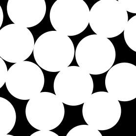
(b) Detail area with negative colours.

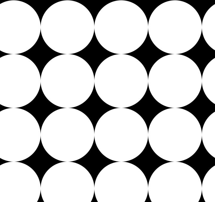
(c) Detail area after homogenization.

Figure 1. Circular polygons in applications: Carbon fiber modelling. (a) Map of the measured locations of the fibres within the resin. (b) As the fibres touch, that is, there is contact, the planar intersections of the cavities form circular $n$-gons. (c) After homogenization, the cavities are circular quadrilaterals. (Data courtesy of I. Babuška, UT Austin.)

Modelling of carbon fibers induces computational domains that are rich in such domains [7]. In Figure 1 a map of measured fiber locations is shown with a detailed image highlighting the domains bounded by aforementioned circular arcs. Notice that due to measurement tolerances it would be correct to assume that all sufficiently small gaps could be modelled as closed, i.e., neighbouring fibers touching each other. In fact, in order to avoid cusps, in [7] a minimum distance between fibers was imposed.

Using domain specific discretizations of computational domains as opposed to traditional triangulations is one of the most active areas of numerical methods for partial differential equations. In particular, we want to mention the virtual element method [12] and the cut finite element method [20]. In our context, of particular interest is the contruction of finite elements on curvilinear polygons or $n$-gons [5]. Constructing quadrature rules for such elements is a challenge, and employing conformal mappings is an intriguing option yet to be fully examined.

Our main goal is to develop numerical methods for calculating conformal moduli of the kind of circular quadrilaterals and $n$-gons mentioned above with as high precision as possible. Both analytic and purely numerical methods are included in this study.

The analytic method (Section 2) uses conformal mappings of the unit disk onto circular quadrilaterals and their Schwarzian derivatives. This method is classical; it is used in many papers including recent ones. Here we should mention the papers [17, 18, 19, 38] concerning the usage of elliptic functions and a spectral Sturm-Liouville problem. The numerical method reduces to a solution of a pair of ordinary differential equations (ODE). In Subsection 2.3, making use of the Riemann–Schwarz symmetry principle, we construct a circular quadrilateral whose modulus can be determined in the analytic form. We use this example for testing accuracy of the developed numerical methods.

The purely numerical method (Section 3) is based on the $hp$-finite element method (FEM) implemented by the first author and previously tested in [31, 33]. In contrast to the first method, the moduli are now computed via potentials of the associated Dirichlet-Neumann problems. The $hp$-FEM results are paired with respective a posteriori error estimates supporting our high confidence in the accuracy of both methods studied here. Two error estimators are considered: The $hp$-FEM a posteriori error estimate based on the auxiliary space methods and the physics based reciprocal error [30, 31]. Convergence in the latter, while general, is only a necessary condition and thus it should always be used in connection with other error estimators. The challenges caused by the zero inner angles are well-known. We deal with this difficulty using geometric mesh grading and control of the order of the polynomial approximation.

The two approaches are compared over a parametrized set of circular quadrilaterals in the form of graphics and tables. The results are in excellent agreement with the analytic results and support our stated goal of being as accurate as possible. The $n$-gon test is carried out with the $hp$-version only. In all cases exponential convergence is achieved with the $hp$-version at the predicted rates [44]. These observations are supported by both types of $hp$-error estimators.

We draw our conclusions in Section 4 and include a sample implementation of the analytic method in the Appendix.

Several authors have studied various topics about conformal mappings of domains with circular arc boundaries. The difficulties encountered already in the case of nonsymmetric quadrilaterals are pointed out in [24, Section 4.10]. The interested reader might want to look at [11, 10, 16, 19, 23, 40].

2. Method of conformal mappings

2.1. Circular quadrilaterals and the Schwarz equation

First we recall some classical results about conformal mapping of canonical domains onto circular polygons.

Let $D$ be a Jordan domain and let its boundary consist of $n$ circular arcs $A_{k-1}A_{k}$, $1\leq k\leq n$ ($A_{0}=A_{n}$). We will name $D$ a circular polygon; the points $A_{k}$ are called the vertices of $D$. Denote by $\alpha_{k}\pi$ the inner angle of $D$ at the vertex $A_{k}$, $0\leq\alpha_{k}\leq 2$.

By definition, the Schwarzian derivative of a meromorphic function $f$ is the expression

$$S_{f}(z)=\left(\frac{f^{\prime\prime}(z)}{f^{\prime}(z)}\right)^{\prime}-\frac{1}{2}\,\left(\frac{f^{\prime\prime}(z)}{f^{\prime}(z)}\right)^{2}.$$

Let now $f$ be a conformal mapping of the unit disk $U:=\{|z|<1\}$ onto $D$ and denote by $a_{k}$ the preimage, under the map $f$, of $A_{k}$ lying on the unit circle $\partial U:=\{|z|=1\}$. The following theorem describes the form of the Schwarzian derivative of $f$ (see, e.g. [27, ch.3, § 1], [37, § 12]).

Theorem 1.

The Schwarzian derivative of the conformal mapping $f$ of $U$ onto the circular polygon $D$ has the form

(1) $$S_{f}(z)=\sum_{k=1}^{n}\frac{(1-\alpha_{k}^{2})/2}{(z-a_{k})^{2}}+\frac{C_{k}}{z-a_{k}}\,.$$

Here the parameters $C_{k}$ are some complex numbers satisfying the relations:

$$\left\{\begin{matrix}\sum_{k=1}^{n}C_{k}=0,\\[5.69054pt] \frac{1}{2}\sum_{k=1}^{n}(1-\alpha_{k}^{2})+\sum_{k=1}^{n}C_{k}a_{k}=0,\\[5.69054pt] \sum_{k=1}^{n}(1-\alpha_{k}^{2})a_{k}+\sum_{k=1}^{n}C_{k}a_{k}^{2}=0.\\ \end{matrix}\right.$$

From Theorem 1 we see that the expression (1) for the Schwarzian derivative of $f$ contains $n$ unknown constants (or so-called accessory parameters) $C_{k}$; finding these constants is a very complicated problem. The problem of determining a function by its given Schwarzian derivative is well known; many papers are devoted to this investigation. Various methods are used to study the problem such as the parametric method [4, 9, 22, 36, 39], boundary value problems [21, 46, 47, 48], Polubarinova-Kochina’s method [13, 14], the method of asymptotic integration [37], and others. (Some of these references point out that the problem of accessory parameters is very important for investigations in fluid mechanics, especially, in the filtration theory.)

If we know the values of $C_{k}$, then the problem of finding $f$ is reduced to solving the nonlinear third order differential equation

$$\left(\frac{f^{\prime\prime}(z)}{f^{\prime}(z)}\right)^{\prime}-\frac{1}{2}\,\left(\frac{f^{\prime\prime}(z)}{f^{\prime}(z)}\right)^{2}=\sum_{k=1}^{n}\frac{(1-\alpha_{k}^{2})/2}{(z-a_{k})^{2}}+\frac{C_{k}}{z-a_{k}}\,.$$

The following theorem gives a connection between the problem and integration of linear second order differential equation (see, e.g. [26, ch.VI], [37, 48]).

Theorem 2.

Let the Schwarzian derivative $S_{f}$ of $f$ be given. Then $f$ is defined by $S_{f}$ up to a Möbius transformation. The general solution of the problem is given by the formula

$$f(z)=\frac{u(z)}{v(z)}\,.$$

Here $u$ and $v$ are arbitrary linear independent solutions of the equation

(2) $$h^{\prime\prime}(z)+(1/2)S_{f}(z)h(z)=0.$$

Remark 1.

Assume that we seek an odd solution to the problem in a domain $G$, containing the origin and symmetric with respect to the origin, and $S_{f}(z)$ is an even function in $G$. Then we can take $u$ and $v$ as odd and even solutions of the equation (2) in $G$. Therefore, we find $u$ and $v$ as solutions to (2) with the following conditions:

(3) $$u(0)=0,\ \ u^{\prime}(0)=C\neq 0,\ \ v(0)=1,\ v^{\prime}(0)=0.$$

2.2. Conformal mapping of symmetric circular quadrilaterals

We apply Theorems 1 and 2 in a special case. Let $A_{1}A_{2}A_{3}A_{4}$ be a circular quadrilateral with zero inner angles symmetric with respect to both the axes. Let the centers of the circles, containing the circular arcs $A_{k-1}A_{k}$, be at points $\pm t$, $\pm is$, where $t$, $s>0$. We also assume that at the points $A_{k}$ the circles touch each other externally (Fig. 2). Denote the radii of circles centered at $\pm t$ and $\pm is$ by $r_{1}$ and $r_{2}$. Then, by Pythagoras’ theorem, $t^{2}+s^{2}=(r_{1}+r_{2})^{2}$.

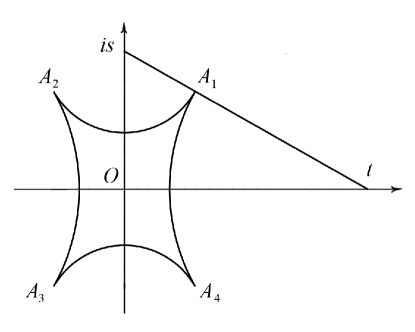
Figure 2. Symmetric circular quadrilateral with zero angles

Denote by $f$ the conformal mapping of the unit disk onto $A_{1}A_{2}A_{3}A_{4}$. Because of the symmetry of the quadrilateral with respect to the coordinate axes and the Riemann–Schwarz symmetry principle, we may assume without loss of generality that

(4) $$f(\overline{z})=\overline{f(z)},\quad f(-z)=-f(z).$$

Therefore, the preimages $a_{k}$ of the vertices $A_{K}$ are symmetric with respect to the axes, i.e. we can put

(5) $$a_{1}=e^{i\beta},\ a_{2}=-e^{-i\beta},\ a_{3}=-e^{i\beta},\ \mbox{\rm and}\ a_{4}=e^{-i\beta},\quad 0<\beta<\pi/2.$$

Because all the angles of the quadrilateral equal zero, we have $\alpha_{k}=0$, $1\leq k\leq 4$. Then, by Theorem 1, the Schwarzian derivative of $f$ has the form

(6) $$S_{f}(z)=\frac{1}{2}\,\left[\frac{1}{(z-e^{i\beta})^{2}}+\frac{1}{(z+e^{-i\beta})^{2}}+\frac{1}{(z+e^{i\beta})^{2}}+\frac{1}{(z-e^{-i\beta})^{2}}\right]\\ +\left[\frac{C_{1}}{z-e^{i\beta}}+\frac{C_{2}}{z+e^{-i\beta}}+\frac{C_{3}}{z+e^{i\beta}}+\frac{C_{4}}{z-e^{-i\beta}}\right]\,;$$

here the constants $C_{k}$, $1\leq k\leq 4$, satisfy

$$C_{1}+C_{2}+C_{3}+C_{4}=0,$$

(7) $$e^{i\beta}C_{1}-e^{-i\beta}C_{2}-e^{i\beta}C_{3}+e^{-i\beta}C_{4}=-2,$$

$$e^{i2\beta}C_{1}+e^{-i2\beta}C_{2}+e^{i2\beta}C_{3}+e^{-i2\beta}C_{4}=0.$$

From the first and third equations of the system we obtain $C_{1}+C_{3}=0$, $C_{2}+C_{4}=0$, therefore $C_{3}=-C_{1}$, $C_{4}=-C_{2}$. From (4) it follows that $C_{4}=\overline{C_{1}}$. Moreover, (7) implies $\mathop{\rm Re}\nolimits[e^{i\beta}C_{1}]=-1/2$.

Denote $\mathop{\rm Im}\nolimits[e^{i\beta}C_{1}]=\delta$. Then

$$e^{i\beta}C_{1}=-1/2+i\delta,\ e^{-i\beta}C_{2}=1/2+i\delta,\ e^{i\beta}C_{3}=1/2-i\delta,\ e^{-i\beta}C_{4}=-1/2-i\delta.$$

After simple transformations we obtain (see also [43])

(8) $$\frac{1}{2}\,S_{f}(z)=\frac{e^{i2\beta}}{(z^{2}-e^{i2\beta})^{2}}+\frac{e^{-i2\beta}}{(z^{2}-e^{-i2\beta})^{2}}-\frac{\gamma}{(z^{2}-e^{i2\beta})(z^{2}-e^{-i2\beta})}$$

where $\gamma=2\delta\sin 2\beta\in\mathbb{R}$.

By Theorem 2, taking into account (4), we represent $f$ in the form

(9) $$f(z)=C\,\frac{u(z)}{v(z)}\,,\quad C>0,$$

where $C$ is a constant and

$$u(z)=z+\sum_{k=2}^{\infty}a_{k}z^{k}+\ldots\ \mbox{\rm and}\ v(z)=1+\sum_{k=1}^{\infty}b_{k}z^{k}$$

are linearly independent solutions to the ODE (2). Taking into account that, by (4), $f$ is odd and $S_{f}$ is an even function, with the help of Remark 1, we conclude that $u(z)$ is odd and $v(z)$ is even. Thus,

(10) $$u^{\prime\prime}(z)+({1}/{2})\,S_{f}(z)u(z)=0,\quad u(0)=0,\ u^{\prime}(0)=1,$$

(11) $$v^{\prime\prime}(z)+({1}/{2})\,S_{f}(z)v(z)=0,\quad v(0)=1,\ v^{\prime}(0)=0.$$

Therefore, we have the following result.

Theorem 3.

Let $f$ be the conformal mapping of the unit disk onto a symmetric circular quadrilateral $Q$ with zero angles such that the points $\pm e^{\pm i\beta}$, $0<\beta<\pi/2$, correspond to the vertices of $Q$. Then the Schwarzian derivative of $f$ is a rational function expressed by (8) with some real $\gamma$, and $f$ has the form (9) where $C$ is a positive constant, and the functions $u$ and $v$ are solutions of the problems (10) and (11).

We should note that the result on the form of the Schwarzian derivative is actually obtained in [43, Appendix] for a more general case. Here we focus on the case of zero angles.

The equations (10) and (11) can be used to find the values of $\beta$ and $\gamma$, corresponding to a given circular quadrilateral $Q=A_{1}A_{2}A_{3}A_{4}$. If we fix some values of parameters $\beta$ and $\gamma$ and solve the boundary problems for ODEs, then we find the mapping $f(z)=Cu(z)/v(z)$ up to a factor $C\neq 0$. The obtained function $f(z)=f(z;\beta,\gamma)$ maps the unit disk onto a symmetric circular quadrilateral, possibly, non-univalently, with zero inner angles. It is evident that for a given symmetric circular quadrilateral $Q$, there is a unique pair $(\beta,\gamma)$ such that $f(z;\beta,\gamma)$, with an appropriate value of $C$, maps the unit disk onto $Q$.

Therefore, the main problem is to find such a pair $(\beta,\gamma)$ for a given $Q$. We note that the parameter $\beta$ has a very simple geometric meaning. Finding $\beta$ is equivalent to finding the conformal modulus of $Q$. Actually, because of the property of conformal invariance, the modulus of $Q$ is equal to the modulus of the unit disk with vertices (5) which depend only on $\beta$. The parameter $\gamma$ has no simple geometric meaning but it also affects the geometry of $Q$.

To find $(\beta,\gamma)$ numerically, we seek $u(e^{i\theta})$ and $v(e^{i\theta})$ as solutions of the following boundary value problems for ODEs:

(12) $$u^{\prime\prime}(re^{i\theta})+\frac{e^{i2\theta}}{2}\,S_{f}(re^{i\theta})u(re^{i\theta})=0,\ 0\leq r\leq 1,\quad u(0)=0,\ u^{\prime}(0)=e^{i\theta},$$

(13) $$v^{\prime\prime}(re^{i\theta})+\frac{e^{i2\theta}}{2}\,S_{f}(re^{i\theta})v(re^{i\theta})=0,\ 0\leq r\leq 1,\quad v(0)=1,\ v^{\prime}(0)=0,$$

and determine $f(e^{i\theta})=Cu(e^{i\theta})/v(e^{i\theta})$. Then we determine the values $T=f(1)$, $S=f(i)/i$, and the values of the radii $R_{1}$ and $R_{2}$ of the circles containing the circular arcs $f(e^{i\theta})$, $-\beta<\theta<\beta$, and $f(e^{i\theta})$, $\beta<\theta<\pi-\beta$. All these values depend on the parameters $\beta$ and $\gamma$. Then we compare the ratios $S/T$ and $R_{2}/R_{1}$ with the given ones, $s/t$ and $r_{2}/r_{1}$. Therefore, we have two equations to determine $\beta$ and $\gamma$:

(14) $$\frac{S(\beta,\gamma)}{T(\beta,\gamma)}=\frac{s}{t}\,,\quad\frac{R_{2}(\beta,\gamma)}{R_{1}(\beta,\gamma)}=\frac{r_{2}}{r_{1}}\,.$$

This system has a unique solution and the obtained value of $\beta$ enables us to find the modulus of $Q$.

Because our main goal is to determine the conformal modulus of $Q$ solving the system (14) and because the ratios $R/T$ and $R_{2}/R_{1}$ do not change under homotheties, below we will often assume that the constant $C$ in (9) equals $1$.

2.3. Example of circular quadrilateral with exactly known modulus

Unfortunately, there are very few examples of concrete circular quadrilaterals with exactly known values of the conformal modulus. In this section, with the help of the Riemann–Schwarz symmetry principle and the Schwarz–Christoffel formula, we give an example of this type.

Consider the circular quadrilateral $Q$, $Q\subset U$, with vertices lying on the unit circle $\partial U$ at the points

$$A_{1}=e^{i\alpha},\ A_{2}=-e^{-i\alpha},\ A_{3}=-e^{i\alpha},\ \mbox{\rm and}\ \ A_{4}=e^{-i\alpha},\quad\alpha=\arcsin{(1/\sqrt{3})}.$$

Let the boundary arcs of $Q$ be orthogonal to the unit circle. The Möbius transformation

$$\omega=(i\cot\alpha)\,\,\frac{e^{-i\alpha}-z}{e^{-i\alpha}+z}\,$$

maps $Q$ conformally onto the circular quadrilateral $D$ lying in the upper half-plane of the variable $\omega$, bounded by two rays, $\{\mathop{\rm Re}\nolimits\omega=-2,\mathop{\rm Im}\nolimits\omega\geq 0\}$, $\{\mathop{\rm Re}\nolimits\omega=1,\mathop{\rm Im}\nolimits\omega\geq 0\}$, and two semicircles, $\{|\omega+1|=1,\mathop{\rm Im}\nolimits\omega\geq 0\}$ and $\{|\omega-1/2|=1/2,\mathop{\rm Im}\nolimits\omega\geq 0\}$ (Fig. 3 (A)). For convenience and brevity of notation, we use the same notations for boundary points corresponding to each other in different complex planes under the applied conformal mappings.

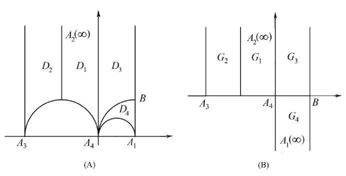
Figure 3. (A) Circular quadrilateral in the upper half-plane;  (B) its strip-shaped image.

Denote by $D_{1}$ the subdomain of $D$ lying in the strip $\{-1<\mathop{\rm Re}\nolimits\omega<0\}$.

Let $F$ be the conformal map of $D_{1}$ onto the half-strip $G_{1}=\{-1<\varphi<0,\psi>0\}$ in the $w$-plane ($w=\varphi+i\psi$) such that $F(-1+i)=-1$, $F(0)=0$, $F(\infty)=\infty$.

Applying the Riemann-Schwarz symmetry principle, we extend the mapping $F$ to the domains $D_{2}$ and $D_{3}$, symmetric to $D_{1}$ with respect to lines $\mathop{\rm Re}\nolimits\omega=-1$ and $\mathop{\rm Re}\nolimits\omega=0$, resp. Then the extended mapping, for which we keep the same notation $F$, maps the union of domains $D_{1}\cup D_{2}\cup D_{3}$ (supplemented with their common boundary arcs) onto the strip $\{-2<\varphi<1\}$ consisting of three half-strips, $G_{1}$, $G_{2}$, and $G_{3}$ (Fig. 3). At last, we can extend, by symmetry, $F$ to the domain $D_{4}$, symmetric to $D_{3}$ with respect to the boundary arc $A_{4}B$, lying on the unit circle $\{|w|=1\}$. The extended function maps conformally $D_{4}$ onto the half-strip $G_{4}$ symmetric to $G_{4}$ with respect to the real axis. As a result, we conclude that the domain $D$ is conformally equivalent to the strip-shaped domain $G$ glued from the half-strips $G_{k}$, $1\leq k\leq 4$, along their common boundary segments.

Let us map conformally the upper half-plane in the $\zeta$-plane onto $G$ such that the points $-1/\lambda$, $-1$, $1$, and $1/\lambda$ ($\lambda>1$) correspond to $A_{2}$, $A_{3}$, $A_{4}$, and $A_{1}$. The desired mapping is given by the Schwarz-Christoffel integral

$$G(\zeta)=c\int_{1}^{\,\zeta}\sqrt{\frac{1-t}{1+t}}\,\,\frac{dt}{1-\lambda^{2}t^{2}}$$

with some constant $c>0$. In a neighborhood of $\zeta=1/\lambda$ we have

(15) $$G(\zeta)\sim i\frac{c}{2\lambda}\sqrt{\frac{1-\lambda}{1+\lambda}}\,\log(\zeta-1/\lambda).$$

By a similar way, as $\zeta\to-1/\lambda$, we have

(16) $$G(\zeta)\sim-i\frac{c}{2\lambda}\sqrt{\frac{1+\lambda}{1-\lambda}}\,\log(\zeta+1/\lambda).$$

We recall that the function $\log(\zeta)$, maps conformally the upper half of a sufficiently small neighborhood of the origin onto a half-strip-like domain of width $\pi$.

Taking into account the values of widths of the half-strip parts of $G$ and the asymptotics (15), (16), we obtain

$$\frac{\pi c}{2\lambda}\sqrt{\frac{1-\lambda}{1+\lambda}}\,=1,\quad\frac{\pi c}{2\lambda}\sqrt{\frac{1+\lambda}{1-\lambda}}\,=3,$$

therefore, $(1+\lambda)/(1-\lambda)=3$ and $\lambda=1/2$.

Now we can find the value of the conformal modulus of $Q$. Because of the invariance of the modulus under conformal mappings, we see that $\mbox{\rm Mod}(Q)$ is equal to the modulus of the quadrilateral which is the upper half-plane with vertices $\pm 1$, $\pm 1/\lambda$. Therefore, it can be computed via elliptic integrals (see, e.g. [3], [6]):

$$(\mbox{\rm Mod}(Q))^{-1}=\frac{2K(\lambda)}{K(\lambda^{\prime})}$$

where

$$K(\lambda)=\int_{0}^{1}\frac{dt}{\sqrt{(1-t^{2})(1-\lambda^{2}t^{2})}}$$

is the complete elliptic integral of the first kind and $\lambda^{\prime}=\sqrt{1-\lambda^{2}}=\sqrt{3}/2$. At last, we obtain

$$\mbox{\rm Mod}(Q)=\frac{K(\sqrt{3}/2)}{2K(1/2)}\,=0.6396307855855...$$

Now we will find the Schwarzian derivative of the conformal mapping of the unit disk onto $Q$. As we noted in Subsection 2.2, it has the form (8). The cross-ratio of a quadruple,

$$(z_{1},z_{2};z_{3},z_{4})=\frac{(z_{3}-z_{1})(z_{4}-z_{2})}{(z_{3}-z_{2})(z_{4}-z_{1})}$$

is invariant under Möbius transformations. Comparing the cross-ratios for vertices of the two quadrilaterals, the first one of which is the unit disk with vertices $\pm e^{\pm i\beta}$ and the second one is the upper half-plane with vertices $\pm 1$, $\pm 1/\lambda$ we obtain

$$\sin\beta=\frac{1-\lambda}{1+\lambda}\,=\frac{1}{3}\,,$$

therefore, $\beta=\arcsin(1/3)$.

Careful analysis of the Schwarzian derivative in small neighborhoods of the points $\pm e^{\pm i\beta}$ shows that, in the considered case, the parameter $\gamma$ in (8) equals $2/3$.

2.4. Conformal mapping of circular $n$-gons

It is of interest to consider circular $n$-gons with $n>4$ and compute moduli of quadrilaterals which are obtained from them after fixing four of their vertices.

Here we give some examples of circular $n$-gons with zero angles and known conformal moduli of quadrilaterals constructed on the base of these $n$-gons; they can be also used for testing the error of the $hp$-FEM in finding conformal moduli (Section 3).

Example 1.

In the $z$-plane, $z=x+iy$, we consider a circular hexagon $H$ with zero angles. The hexagon is obtained from the half-strip $\{-2<x<2,y>0\}$ by removing points lying in the disks $\{(x+1)^{2}+y^{2}\leq 1$, $\{(x-1/3)^{2}+y^{2}\leq 1/9\}$, $(x-5/6)^{2}+y^{2}\leq 1/36\}$, $\{(x-3/2)^{2}+y^{2}\leq 1/4\}$. It has vertices at the points (Fig. 4 (A))

$$A(-2,0),\,B(0,0),\,C(2/3,0),\,D(1,0),\,E(2,0),\,\,{\rm and}\,\,F(\infty)\,.$$

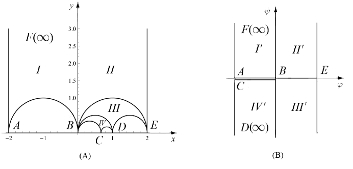
Figure 4. (A) Circular hexagon in the upper half-plane;  (B) its polygonal image.

Let us map conformally the circular triangle $I:=\{-2<x<0,y>0\}\setminus\{(x+1)^{2}+y^{2}\leq 1\}$ onto the half-strip $I^{\prime}:=\{-\pi/2<\varphi<0,\psi>0\}$ in the $w$-plane, $w=\varphi+i\psi$. Applying three times the Riemann-Schwarz symmetry principle, we extend the mapping step by step to the circular triangles designated on the Fig. 4 (A), by $I\!I$, $I\!I\!I$, and $IV$. The extended function $f$ maps the triangles onto the half-strips $I\!I^{\prime}$, $I\!I\!I^{\prime}$, and $IV^{\prime}$ (Fig. 4 (B)).

Therefore, $f$ maps conformally $H$ onto the strip $\{|\varphi|<\pi/2\}$ with the slit along the segment $\{-\pi/2<\varphi<0,\,\psi=0\}$. Denote this domain by $\Omega$. The function $\omega=g(w):=2\sin w-1$ maps conformally $\Omega$ onto the $\omega$-plane, $\omega=\xi+i\eta$ with two slits along the rays $\{\xi\leq-1,\,\eta=0\}$ and $\{\xi\geq 1,\,\eta=0\}$. Then we apply the function inverse to the Joukowsky function: $\sigma=h(\omega)=\omega+\sqrt{\omega^{2}-1}$ with an appropriate choice of regular branch of the square root. The composition $h\circ g\circ f$ maps conformally the hexagon $H$ onto the upper half-plane with the following correspondence of the points:

(17) $$A\mapsto-(3+2\sqrt{2}),B\mapsto-1,C\mapsto-(3-2\sqrt{2}),D\mapsto 0,E\mapsto 1,F\mapsto\infty.$$

Therefore, we have the following result.

The hexagon $H$ is conformally equivalent to the upper half-plane with the correspondence of points given by (17).

Because the conformal modulus of the quadrilateral which is the upper half-plane with four fixed vertices on the real axis is well-known, we can fix any four of the six vertices and easily compute the modulus of the obtained quadrilateral.

Remark 2.

In Section 3 we use this example to verify the accuracy of the $hp$-FEM for determining conformal moduli of circular $n$-gons. This method needs calculation of double integrals over a given $n$-gon, therefore, it is better to apply it in a bounded domain. Since the modulus is a conformal invariant, we can consider, instead of the unbounded hexagon $H$, its conformal image under the Möbius transformation

$$w=T(z)=\frac{4-(1-3i)z}{4-(1+3i)z}\,.$$

This transformation maps the upper half-plane onto the unit disk; and $Q$ corresponds to the hexagon bounded by circular arcs orthogonal to the unit circle. Moreover, there is the following correspondence between the vertices of $Q$ and their images:

$$A\mapsto-i,\ B\mapsto 1,\ C\mapsto\frac{8+15i}{17}\,,\ D\mapsto i,\ E\mapsto\frac{-4+3i}{5}\,,\ F\mapsto\frac{-4-3i}{5}\,.$$

The obtained hexagon is considered in Subsubsection 3.3.3 (see Fig. 6).

Example 2.

Given $n\geq 4$, consider the circular $n$-gon $P_{n}$ which is obtained from the half-strip

$$\{0<x<2(n-2),y>0\}$$

by removing the disks $D_{k}:=\{(x-(2k-1))^{2}+y^{2}\leq 1\}$, $1\leq k\leq n-2$. It has zero angles and vertices at the points $0$, $2$, $4$,…,$2n-2$, $\infty$. We map the triangle $\{0<x<2,y>0\}\setminus D_{1}$ onto the half-strip $\{0<\varphi<2,\psi>0\}$ and extend the mapping by symmetry to a conformal mapping of the $n$-gon onto the half-strip $S:=\{0<\varphi<2(n-2),\psi>0\}$. Then we map $S$ onto the upper half-plane by the function $\zeta=-\cos\frac{\pi w}{2(n-2)}$. Then the vertices of $P_{n}$ are mapped to the points $-\cos\frac{\pi k}{n-2}$, $k=0,1,\ldots,n-2$, and $\infty$. As in Example 1, fixing four vertices of $P_{n}$ we can find exact value of modulus of the obtained quadrilateral.

2.5. Numeric results

Here we give a numerical algorithm to find the values of $\beta$ and $\gamma$ in (8) for a given symmetric quadrilateral with zero inner angles (see Fig.2). For this, as indicated above, we need to solve the system (14).

Denote $k:=s/t$, $K:=r_{2}/r_{1}$. Then (14) has the form

(18) $$S(\beta,\gamma)/T(\beta,\gamma)=k,\quad R_{2}(\beta,\gamma)/R_{1}(\beta,\gamma)=K.$$

First we describe how, for given arbitrary $\beta$ and $\gamma$, to find the centers, $T(\beta,\gamma)$ and $iS(\beta,\gamma)$, and the radii, $R_{1}(\beta,\gamma)$ and $R_{2}(\beta,\gamma)$, of circles which contains the boundary circular arcs of the corresponding circular polygon. We note that boundary arcs are symmetric with respect to either the real or the imaginary axis, therefore, it is sufficient to determine two distinct points for each of the circles. We can find $f(e^{i\theta})=u(e^{i\theta})/v(e^{i\theta})$, solving the equations (12) and (13), where $S_{f}$ is defined by (8) and corresponds to the fixed values of $\beta$ and $\gamma$. Then we take two different values of $\theta$ from $[0,\beta)$, say, $\theta_{1}=0$ and $\theta_{2}=\beta/2$, and find the values of $f(e^{i\theta_{1}})$ and $f(e^{\theta_{2}})$. Let $x_{1}=f(e^{i\theta_{1}})$ and $x_{2}+iy_{2}=f(e^{\theta_{2}})$. Next we determine

$$T=(1/2)(x_{1}+x_{2}+y_{2}^{2}/(x_{2}-x_{1})),\ R_{1}=|t-x_{1}|$$

where $x_{1}=f(e^{i\theta_{1}})$ and $x_{2}+iy_{2}=f(e^{\theta_{2}})$. By a similar way, we fix two angles in $(\beta,\pi/2]$, say, $\theta_{3}=\pi/4+\beta/2$ and $\theta_{4}=\pi/2$, and find

$$S=(1/2)(y_{3}+y_{4}+x_{4}^{2}/(y_{4}-y_{3})),\ R_{2}=|s-y_{4}|,$$

where $x_{3}+iy_{3}=f(e^{i\theta_{3}})$, $iy_{4}=f(e^{\theta_{4}})$.

Now we describe how to solve the system (18). Initially, for a given fixed $\beta$, we solve the first equation from (18) with respect to $\gamma$. We should note that for given values of $\beta$ and $k$, a symmetric circular quadrilateral and, therefore, $\gamma$ are not uniquely determined. We consider circular polygons such that the circles, containing their boundary, touch each other externally at intersection points. But there could be another circular polygon with the same values of $\beta$ and $k$ and the circles touching internally. To avoid this, first, for a given $\beta$ we need to determine the values of $\gamma$, $A_{\gamma}$ and $B_{\gamma}$, $A_{\gamma}<B_{\gamma}$, for which we obtain circular quadrilaterals with a pair of sides lying on parallel straight lines. The values $A_{\gamma}$ and $B_{\gamma}$ correspond to the conditions $x_{1}=0$ ($R_{1}=\infty$) and $y_{4}=0$ ($R_{2}=\infty$).

We find the values of $A_{\gamma}$ and $B_{\gamma}$ by the bisection method on some segment $I=[a_{\gamma},b_{\gamma}]$. The segment $I$ must be sufficiently large and contain $A_{\gamma}$ and $B_{\gamma}$. Using a numerical experiment, we determined that for a wide class of $\beta$ and $k$ the following values of the parameters are appropriate:

$$a_{\gamma}=0.7-(4/\pi)\beta,\quad b_{\gamma}=1.2-(3/\pi)\beta.$$

When the values of $A_{\gamma}$ and $B_{\gamma}$ are found, we determine the desired value of $\gamma=\gamma(\beta)$.

To fulfill the second equality in (18), we solve the equation

$$R_{2}(\beta,\gamma(\beta))/R_{1}(\beta,\gamma(\beta))=K$$

making use of the bisection method on the segment $[0,\pi/4]$. We do not know a priori, whether $\beta<\pi/4$ (this means that the modulus is less than $1$). If it turns out that the numerical value of the desired modulus is greater than $1$ and, therefore, $\beta\geq\pi/4$, then the bisection method on the segment $[0,\beta/4]$ converges to the boundary value $\beta=\pi/4$. In this case, we swap the values of $t$ and $s$, as well as $r_{1}$ and $r_{2}$, and repeat the calculations for these updated values; at the end, the found value of $\beta$ must be changed to $\pi/2-\beta$.

For numeric calculations we used the Wolfram Mathematica software. If we want to obtain the approximate value of the modulus quickly and with accuracy about $10^{-6}$, for solving Cauchy’s problems for differential equations with the help of NDSolve we can use the option ’PrecisionGoal$-\!\!\!>$15. To find the parameters $A_{\gamma}$ and $B_{\gamma}$ with the help of the bisection method, it is sufficient to use 10 iterations; and for each of the parameters, $\beta$ and $\gamma$, we used 25 iterations.

In Appendix A we give the Mathematica code for calculation of conformal moduli. The input values of $t$, $s$, $r_{1}$, and $r_{2}$ (lines 1–4) match to the example 2) below with $\alpha=\pi/5$, $j=3$. The output is the found values of $\mbox{\rm Mod}(Q)$, $\beta$ and $\gamma$ (line 118).

If we need a higher accuracy, we can first find the approximate values $\beta$ and $\gamma$ with accuracy $10^{-6}$. Denote them by $\beta_{0}$ and $\gamma_{0}$. Then we use the bisection method with respect to $\beta$ and $\gamma$ assuming that $\beta\in[\beta_{0}-\varepsilon,\beta_{0}+\varepsilon]$ and $\gamma\in[\gamma_{0}-\varepsilon,\gamma_{0}+\varepsilon]$ with sufficiently small $\varepsilon$, say $\varepsilon=2\cdot 10^{-6}$. Certainly, in the case, we omit the first two steps connected with finding the values of $A_{\gamma}$ and $B_{\gamma}$. To find $\beta$ and $\gamma$, we use NDSolve with option ’PrecisionGoal$-\!\!\!>$30; for each of the parameters, the number of iterations is $30$. With this enhanced method, the accuracy is about $10^{-10}-10^{-11}$ though it needs much more computing time (a few minutes instead of 10–15 seconds).

Now we give numerical results.

1) For $k=\sqrt{2}$ and $K=2$ we know the exact values $\beta=\arcsin(1/3)$, $\gamma=2/3$ (see Subsection 2.3).

Using the options PrecisionGoal$-\!\!\!>$15, WorkingPrecision$-\!\!\!>$30 with the number of steps equals 30 for each of the parameters, we find that the approximate values are

$$\sin\beta=0.3333333333332441,\quad\gamma=0.666666666666788.$$

Therefore, the absolute error is about $1.2\cdot 10^{-13}$.

2) Assume that the vertex $A_{1}$ is $e^{i\alpha}$, $\alpha=\pi/n$, $n\in\mathbb{N}$, $4\leq n\leq 8$ (Fig.2). For every $n$ we consider the following five values of $t$:

$$t=1+0.2j(1/\cos\alpha-1),\quad 1\leq j\leq 5.$$

Then

$$s=\frac{t\sin\alpha}{t-\cos\alpha}\quad r_{1}=|e^{i\alpha}-t|,\quad r_{2}=|e^{i\alpha}-is|.$$

We computed the values of conformal modulus for these 25 cases. In Table 1 we give the values obtained with rough accuracy, with higher accuracy, and by the $hp$-FEM (see Section 3). We see that for given $\theta$, the difference in results, given in the fourth (higher accuracy) and fifth ($hp$-FEM variant) columns does not exceed $5\cdot 10^{-10}$. This indicates fairly good accuracy of the suggested methods.

We note that in Subsubsection 3.3.3 two the following cases are considered in more detail: $n=4$, $j=1$ (quadrilateral $Q_{1}$) and $n=8$, $j=5$ (quadrilateral $Q_{2}$).

Table 1. The values of moduli of circular quadrilaterals.

$\alpha$	j	rough accuracy	higher accuracy	$hp$-FEM
$\pi/4$	1	$\phantom{h}1.65195637087856\phantom{h}$	$\phantom{h}1.65195641811156\phantom{h}$	$\phantom{h}1.65195641811801\phantom{h}$
	2	$1.41312892318176$	$1.41312882432748$	$1.41312882433334$
	3	$1.23851630005081$	$1.23851628549016$	$1.23851628549600$
	4	$1.10517568205164$	$1.10517573064876$	$1.10517573065505$
	5	$\!\!\!\!\!\!1.$ (sharp value)	$\!\!\!\!\!\!1.$ (sharp value)	$1.00000000000704$
$\pi/5$	1	$0.98160716203795$	$0.98160730939538$	$0.98160730941547$
	2	$0.88131392216865$	$0.88131392866493$	$0.88131392869094$
	3	$0.79679231514866$	$0.79679236427334$	$0.79679236430546$
	4	$0.72458905475484$	$0.72458889240001$	$0.72458889243949$
	5	$0.66218846198336$	$0.66218813398119$	$0.66218813402464$
$\pi/6$	1	$0.69813401618400$	$0.69813355689778$	$0.69813355697485$
	2	$0.63911291428315$	$0.63911229266297$	$0.63911229274088$
	3	$0.58614443760266$	$0.58614411420414$	$0.58614411428162$
	4	$0.53833141064728$	$0.53833144748697$	$0.53833144756331$
	5	$0.49493995006987$	$0.49493951440663$	$0.49493951447948$
$\pi/7$	1	$0.54204363753707$	$0.54204377899126$	$0.54204377906567$
	2	$0.50133118737030$	$0.50133063755764$	$0.50133063763325$
	3	$0.46350927171723$	$0.46350872114770$	$0.46350872122462$
	4	$0.42826417448376$	$0.42826373909062$	$0.42826373916846$
	5	$0.39531876405162$	$0.39531863465020$	$0.39531863472915$
$\pi/8$	1	$0.44327621319647$	$0.44327582367411$	$0.44327582393810$
	2	$0.41254694695236$	$0.41254658974644$	$0.41254659003158$
	3	$0.38338345187308$	$0.38338339855016$	$0.38338339885322$
	4	$0.35565053319540$	$0.35565066792949$	$0.35565066823961$
	5	$0.32922105387009$	$0.32922144646084$	$0.32922144678543$

3. Moduli via potentials

The finite element method (FEM) is the standard numerical method for solving elliptic partial differential equations. Since FEM is an energy minimization method it is eminently suitable for problems involving Dirichlet energy. In the context of this paper where the focus is on domains with zero inner angles at the vertices, the $hp$-FEM variant is the most efficient one [8, 44]. With proper grading of the meshes even with uniform polynomial order exponential convergence can be achieved even in problems with strong corner singularities.

In this section we give a brief overview of the method and our implementation [31, 33]. Of particular importance is the possibility to estimate the error in the computed quantity of interest. For quadrilaterals there exists a natural error estimate, the so-called reciprocal relation which is a necessary but not sufficient condition for convergence. However, if the reciprocal relation is coupled with a posteriori error estimates, we can trust the results with high confidence [30].

3.1. Modulus of quadrilateral and the Dirichlet integral

Let $Q=(Q;z_{1},z_{2},z_{3},z_{4})$ be a quadrilateral and the boundary $\partial Q=\cup_{k=1}^{4}\partial Q_{k}$ where all four boundary arcs are assumed to be non-degenerate. Consider the following Dirichlet-Neumann problem already introduced in the introduction:

(19) $$\left\{\begin{matrix}\Delta u&=&\ 0,&\text{on}\ &{\ Q,}\\ u&=&\ 1,&\text{on}\ &{\partial Q_{1},}\\ u&=&\ 0,&\text{on}\ &{\partial Q_{3},}\\ \partial u/\partial n&=&\ 0,&\text{on}\ &{\partial Q_{2},}\\ \partial u/\partial n&=&\ 0,&\text{on}\ &{\partial Q_{4}.}\\ \end{matrix}\right.$$

Assume that $u$ is a (unique) harmonic solution of the Dirichlet-Neumann problem (19). Then the modulus of $Q$ is defined as

(20) $$\mbox{\rm Mod}(Q)=\iint_{\Omega}|\nabla u|^{2}\,dx\,dy.$$

The equality (20) shows that the modulus of a quadrilateral is the Dirichlet integral, i.e., the $H^{1}$-seminorm of the potential $u$ squared, or, the energy norm squared, a quantity of interest which is natural in the FEM setting.

3.2. Mesh refinement and exponential convergence

The idea behind the $p$-version is to associate degrees of freedom to topological entities of the mesh in contrast to the classical $h$-version where it is to mesh nodes only. The shape functions are based on suitable orthogonal polynomials and their supports reflect the related topological entity, nodes, edges, faces (in 3D), and interior of the elements. The nodal shape functions induce a partition of unity.

In many problem classes it can be shown that if the mesh is graded appropriately the method convergences exponentially in some general norm such as the $H^{1}$-seminorm. Moreover, due to the construction of shape functions, it is natural to have large curved elements in the mesh without significant increase in the discretization error. Since the number of elements can be kept relatively low given that additional refinement can always be added via elementwise polynomial degree, variation in the boundary can be addressed directly at the level of the boundary representation in some exact parametric form.

To fully realize the potential of the $p$-version, one has to grade the meshes properly and therefore we really use the $hp$-version here. Consider the meshes in Figures 6 and 5. In Figures 6 the basic refinement strategy is illustrated. We start with an initial mesh, where the corners with singularities are isolated, that is, the subsequent refinements of their neighboring elements do not interfere with each other. Then the mesh is refined using successive applications of replacement rules.

(a) Q1: Mesh; $\alpha=\pi/4$.

(b) Q2: Mesh; $\alpha=\pi/8$.

Figure 5. Circular quadrilaterals. Pure $p$-version meshes.

In our implementation the geometry can be described in exact arithmetic and therefore there are not any fixed limits on the number of refinement levels. In the case of graded meshes one has to resolve the question of how to set the polynomial degrees at every element, indeed, a form of refinement of its own. One option in the case of strong singularities is to set the polynomial degree based on graph distance from the singularity. Alternatively, the degree $p$ can be constant over the whole mesh despite the grading.

(a) Initial mesh.

(b) After two levels of refinement.

(c) Potential of the problem.

(d) Potential of the conjugate problem.

Figure 6. Circular hexagon.

3.3. Error estimation

Assuming that the exact capacity is not known, we have two types of error estimates available: the reciprocal estimate and an a posteriori estimate. Naturally, if the exact value is known, we can measure the true error.

3.3.1. Reciprocal Error Estimate

The first error estimate is rather unusual in the sense that it is based on physics, yet only necessary. For every quadrilateral the so-called reciprocal relation can be used (Definition 1). More detailed, from the definition of modulus via conformal mapping it is clear that the following reciprocal identity holds:

(21) $$\mbox{\rm Mod}(Q)\,\mbox{\rm Mod}(\tilde{Q})=1;$$

here $\tilde{Q}=(Q;z_{2},$ $z_{3},z_{4},z_{1})$ is called the quadrilateral conjugate to $Q=(Q;z_{1},z_{2},z_{3},z_{4})$. In numerical context (21) gives us the following error characteristics.

Definition 1.

(Reciprocal Identity and Error) We will call

$$\varepsilon_{R}=|1-\mbox{\rm Mod}(Q)\,\mbox{\rm Mod}(\tilde{Q})|$$

the error measure and $\varepsilon_{N}=\left|\lceil\log_{10}|\varepsilon_{R}|\rceil\right|$ the related error number.

3.3.2. Auxiliary Space Error Estimate

Consider the abstract problem setting with $u$ as the standard piecewise polynomial finite element space on some discretization $T$ of the computational domain $D$. Assuming that the exact solution $u\in H_{0}^{1}(D)$ has finite energy, we arrive at the approximation problem: Find $\hat{u}\in V$ such that

(22) $$a(\hat{u},v)=l(v)\ (=a(u,v))\quad(\forall v\in V),$$

where $a(\,\cdot\,,\,\cdot\,)$ and $l(\,\cdot\,)$, are the bilinear form and the load potential, respectively. Additional degrees of freedom can be introduced by enriching the space $V$. This is accomplished via introduction of an auxiliary subspace or “error space” $W\subset H_{0}^{1}(D)$ such that $V\cap W=\{0\}$. We can then define the error problem: Find $\varepsilon\in W$ such that

(23) $$a(\varepsilon,v)=l(v)-a(\hat{u},v)(=a(u-\hat{u},v))\quad(\forall v\in W).$$

This is simply a projection of the residual to the auxiliary space. In 2D the space $W$, that is, the additional unknowns, can be associated with element edges and interiors. Thus, for $hp$-methods this kind of error estimation is natural. The main result on this kind of estimators is the following theorem.

Theorem 4 ([30]).

There is a constant $K$ depending only on the dimension $d$, polynomial degree $p$, continuity and coercivity constants $C$ and $c$, and the shape-regularity of the triangulation $\mathcal{T}$ such that

$$\frac{c}{C}\,\|\varepsilon\|_{1}\leq\|u-\hat{u}\|_{1}\leq K\left(\|\varepsilon\|_{1}+\mathrm{osc}(R,r,\mathcal{T})\right),$$

where the residual oscillation depends on the volumetric and face residuals $R$ and $r$, and the triangulation $\mathcal{T}$.

The solution $\varepsilon$ of (23) is called the error function. It has many useful properties for both theoretical and practical considerations. In particular, the error function can be numerically evaluated and analyzed for any finite element solution. By construction, the error function is identically zero at the mesh points. In the examples below, the space $W$ contains edge shape functions of degree $p+1$ and internal shape functions of $p+1$ and $p+2$. This choice is not arbitrary but based on careful cost analysis [30].

3.3.3. Examples

The numerical examples are defined in Table 2. We consider in detail two circular quadrilaterals and one hexagon. The related results of Table 1 above have been obtained with the method discussed here.

Example	Parameters or coordinates
$Q_{1}$	$\alpha=\pi/4$, $t=\frac{1}{5}\left(4+\sqrt{2}\right)$, $s=\frac{1}{23}\left(20+19\sqrt{2}\right)$,
	$r_{1}=\frac{1}{5}\sqrt{33-12\sqrt{2}}$, $r_{2}=\frac{1}{23}\sqrt{777+300\sqrt{2}}$
$Q_{2}$	$\alpha=\pi/8$, $t=\sec\left(\frac{\pi}{8}\right)$, $s=\csc\left(\frac{\pi}{8}\right)$,
	$r_{1}=\tan\left(\frac{\pi}{8}\right)$, $r_{2}=1+\sqrt{2}$
hexagon	$A^{\prime}=-i$, $B^{\prime}=1$, $C^{\prime}=\frac{8}{17}+\frac{15}{17}\,i$,
	$D^{\prime}=i$, $E^{\prime}=-\frac{4}{5}+\frac{3}{5}\,i$, $F^{\prime}=-\frac{4}{5}-\frac{3}{5}\,i$

(a) Geometry definitions.

Example	Problem	Conjugate
hexagon	$Q=(Q;A^{\prime},B^{\prime},D^{\prime},E^{\prime})$	$\tilde{Q}=(Q;B^{\prime},D^{\prime},E^{\prime},A^{\prime})$

(b) Problem definitions.

Table 2. Examples: Parameters or coordinates used to define the problems. The problem for hexagon is obtained from Example 1 (cf. Figure 4 (A)) after carrying out the Möbius transformation of Remark 2.

In Figures 7 and 8 different error measures and the related convergence in $p$ are shown. In all cases exponential convergence is realized. The estimated rates obtained through nonlinear fitting are also indicated (with dashed lines) and the parameters used are given in Table 3. One has to remember that such fits are notoriously sensitive to selected points and thus, the rates given here should be taken as possible rates rather than the definitive ones. We have used the visualization technique where the scaling is selected to be such that the observed graph appears linear.

For the two quadrilaterals $Q_{1}$ and $Q_{2}$ the results are very good indeed. In fact, the estimated rate for the $Q_{1}$ is the theoretically optimal one in terms of the number of degrees of freedom, of course with a large constant [44]. The reason behind such a spectacular accuracy is that the underlying mapping of the curved elements, the blending function mapping, is exact for circular boundary segments. From the point of view of the method the corner singularity is practically removed by the mapping. For the $Q_{2}$ with a smaller aspect ratio, at higher polynomial orders there is degradation of the convergence rate in comparison to the symmetric domain of $Q_{1}$, and indeed, the selected scaling cannot remain the same as for $Q_{1}$. Notice that the exceedingly large constant $a_{1}$ for the estimated error is due to the non-trivial oscillation in the estimate and asymptotic convergence reached only at high values of $p$. Due to symmetry, $\mbox{\rm Mod}(Q_{1})=1$. We have not shown the error in capacity in this case. It is done in the following case, however.

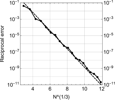
(a) Q1: Reciprocal error; $c=1/3$.

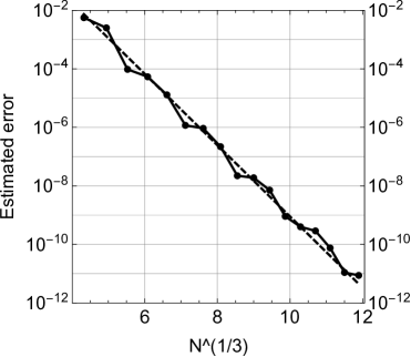
(b) Q1: Estimated error; $c=1/3$.

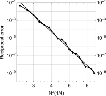
(c) Q2: Reciprocal error; $c=1/4$.

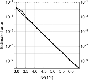
(d) Q2: Estimated error; $c=1/4$.

Figure 7. Circular quadrilaterals. Different types of errors vs the number of degrees of freedom (log-plots). Solid line with markers represents the observed errors and the dashed line fitted exponential curve (rate $c$ indicated in the caption).

For the circular hexagon the geometric meaning of the domain and its conjugate is illustrated in Figures 6c and 6d. In this case the exact modulus is also known,

$$\mbox{\rm Mod}(Q)=\tau(\sqrt{2})/2=\frac{K(1/\sqrt{1+\sqrt{2}})}{K(\sqrt{\sqrt{2}/(1+\sqrt{2})})}\approx 0.92401502327430725964\ldots,$$

where $K(r)$ is the complete elliptic integral. The method is indeed very accurate and the observed rate is within the expected range. As is often the case, the auxiliary space estimate trails the true error, yet the effectivity is still over 1/10 as $p$ increases. Due to the construction of the auxiliary space, the estimate is computed at a lower polynomial order.

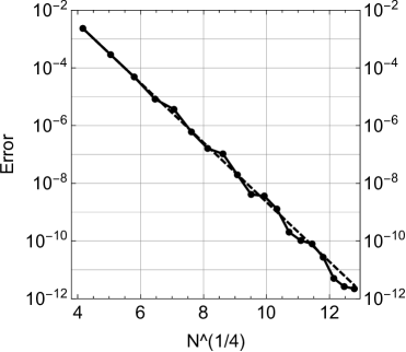
(a) Error in capacity; $c=1/4$.

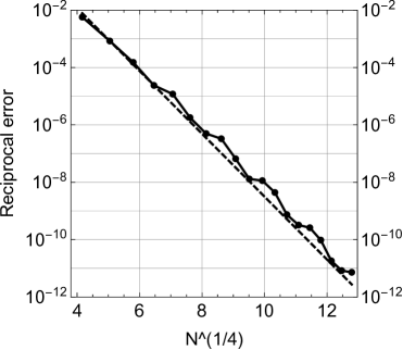
(b) Reciprocal error; $c=1/4$.

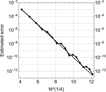
(c) Estimated error; $c=1/4$.

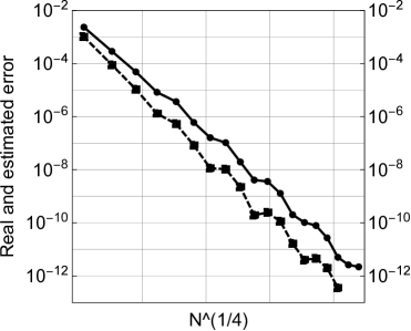
(d) Comparison of the real and estimated errors.

Figure 8. Circular hexagon. Different types of errors vs the number of degrees of freedom (log-plots). Solid line with markers represents the observed errors and the dashed line fitted exponential curve (rate $c$ indicated in the caption). In the comparison graph the estimated error is smaller with asymptotic effectivity of 1/10.

In Table 3 the error numbers for the reciprocal error estimates are also reported for the highest polynomial order. These results are aligned with those reported on similar problems before [32].

Example	Error Type	$a_{1}$	$a_{2}$	$c$	$N$ $(p=20)$	Error Number
$Q_{1}$	Estimated	1397	-2.8	1/3	1681
	Reciprocal	198	-2.6	1/3	1681	10
$Q_{2}$	Estimated	179191	-5.5	1/4	1681
	Reciprocal	2154	-4.4	1/4	1681	9
hexagon	True	47	-2.4	1/4	26761
	Estimated	105	-2.8	1/4	$(p=18)$ 21709
	Reciprocal	287	-2.5	1/4	26761	11

Table 3. Parameters of the nonlinear fits: $a_{1}\operatorname{exp}({a_{2}N^{c}})$, where $N$ is the number of degrees of freedom, and the error numbers for the reciprocal errors.

Remark 3 (On Computational Complexity of the Error Estimates).

The two error estimates do not differ in their computational complexity in any significant way. Although the reciprocal error estimate requires the solution of two problems, and the auxiliary space estimate is for one problem only, the cost of numerical integration (always an issue in high order methods) is roughly the same, and the two solution steps for the reciprocal error estimate can share the Cholesky factorization of the interior degrees of freedom.

Remark 4 (On Performance Comparison Between Schwarz ODE and $hp$-FEM).

As mentioned above, the quadrilateral example is particularly well-suited to the $hp$-FEM. This makes it somewhat awkward to compare the computational efficiency of the two numerical approaches presented in this paper. Of course, one should also take into account the time spent in defining the computational domain. This is very difficult to measure, however. The Schwarz ODE routine and the $hp$-solver have comparable performance when the former is run using standard precision. Due to the implementation of the ODE solver, the higher accuracy is obtained only by changing the floating point representation which leads to longer run times. On the other hand, the Schwarz ODE has an almost uniform runtime characteristics over all circular quadrilaterals and it is likely that replacing the general ODE solver routines with problem specific ones will lead to significant improvements in run times. The $hp$-FEM requires more resources if the discretization includes more elements. With the current $hp$-implementation the non-graded discretization of the $n$-gon (Figure 6a) took three times longer than the corresponding quadrilaterals (Figure 5).

4. Conclusions

Here moduli of planar circular quadrilaterals symmetric with respect to both the coordinate axes have been investigated. Computation of moduli of planar domains with cusps is difficult and requires either a customized, analytic algorithm or general method with sufficient flexibility. The Schwarz ODE introduced here, an analytic method to determine a conformal mapping the unit disk onto a given circular quadrilateral, belongs to the first category. $hp$-FEM on the other hand provides a framework for highly efficient numerical PDE solvers. We have shown that these two different approaches provide results agreeing with high accuracy over two sets of parametrized examples.

Appendix A Reference Implementations

The programs used to compute the Table 1 are available at

https://github.com/hhakula/hnv

and Version 1.0, used in this paper, is archived at DOI: 10.5281/zenodo.4718320.

The Schwarz ODE code is also listed below. The expected output of the program is

$$\{1.02791,0.440765,1.25503\}.$$

Listing 1: Schwarz ODE

⬇

1 t = 2.0174131664886366‘;

2 s = 1.1416407864998739‘;

3 r1 = 1.642663833605752‘;

4 r2 = 0.6753740370343625‘;

5 Clear[K, b, gamma];

6 K = r2/r1;

7 k = s/t;

8mod = 1.;

9While[Abs[mod - 1.] < 10^(-5),

10ba = 0.;

11bb = Pi/4;

12 Do[Clear[gamma,b];

13 b = (ba + bb)/2.;

14 theta1 = 0;

15 theta2 = b/2.;

16 theta3 = Pi/2*(1/2) + b*(1/2);

17 theta4 = Pi/2.;

18 agamma = 0.7 - 4./Pi*b;

19 bgamma = 1.2 - 3./Pi*b;

20 F[x_, beta_, theta_, gamma_] = Exp[2*I*theta](Exp[2*I*beta]/(x^2*Exp[2*I*theta]

21 -Exp[2*I*beta])^2 +Exp[-2*I*beta]/(x^2*Exp[2*I*theta] - Exp[-2*I*beta])^2

22 - gamma (1/((x^2*Exp[2*I*theta] - Exp[2*I*beta])(x^2*Exp[2*I*theta]

23 -Exp[-2*I*beta]))));

24 Do[gamma = (agamma + bgamma)/2.;

25 sol3 = NDSolve[{

26 u3”[x]+F[x,b,theta3,gamma]*u3[x]==0,v3”[x]+F[x,b,theta3,gamma]*v3[x]==0,

27 u3[0]==0,u3’[0]==Exp[I*theta3],v3[0]==1,v3’[0]==0},{u3,v3},{x,0,1}];

28 sol4 = NDSolve[{

29 u4”[x]+F[x,b,theta4,gamma]*u4[x]==0,v4”[x]+F[x,b,theta4,gamma]*v4[x]==0,

30 u4[0]==0,u4’[0]==Exp[I*theta4],v4[0]==1,v4’[0]==0},{u4,v4},{x,0,1}];

31 F3[x_] = u3[x]/v3[x] /. sol3;

32 F4[x_] = u4[x]/v4[x] /. sol4;

33 x2 = Re[F3[1]];

34 y2 = Im[F3[1]];

35 y3 = Im[F4[1]];

36 S = (1/2)(y2+y3+x2^2/(y2-y3));

37 If[ S[[1]]<0,

38 bgamma = gamma,

39 agamma = gamma

40 ],{i, 10}];

41 BGAMMA = gamma;

42 Clear[gamma];

43 agamma = 0.75-4./Pi*b;

44 bgamma = 1.2-3./Pi*b;

45 Do[gamma = (agamma + bgamma)/2.;

46 sol1 = NDSolve[{

47 u1”[x]+F[x,b,theta1,gamma]*u1[x]==0,v1”[x]+F[x,b,theta1,gamma]*v1[x]==0,

48 u1[0]==0,u1’[0]==Exp[I*theta1],v1[0]==1,v1’[0]==0},{u1, v1},{x,0,1}];

49 sol2 = NDSolve[{

50 u2”[x]+F[x,b,theta2,gamma]*u2[x]==0,v2”[x]+F[x,b,theta2,gamma]*v2[x]==0,

51 u2[0]==0,u2’[0]==Exp[I*theta2],v2[0]==1,v2’[0]==0},{u2,v2},{x,0,1}];

52 F1[x_] = u1[x]/v1[x] /. sol1;

53 F2[x_] = u2[x]/v2[x] /. sol2;

54 x1 = Re[F1[1]];

55 x2 = Re[F2[1]];

56 y2 = Im[F2[1]];

57 T = (1/2)(x1+x2+y2^2/(x2-y1));

58 If[ T[[1]] > 0,

59 bgamma = gamma,

60 agamma = gamma

61 ], {i, 10}];

62 AGAMMA = gamma;

63 Clear[gamma,x1,x2,y2,x3,y3,y4];

64 Do[gamma = (AGAMMA + BGAMMA)/2.;

65 sol1 = NDSolve[{

66 u1”[x]+F[x,b,theta1,gamma]*u1[x]==0,v1”[x]+F[x,b,theta1,gamma]*v1[x]==0,

67 u1[0]==0,u1’[0]==Exp[I*theta1],v1[0]==1,v1’[0]==0},{u1,v1},{x,0,1},

68 PrecisionGoal->15];

69 sol2 = NDSolve[{

70 u2”[x]+F[x,b,theta2,gamma]*u2[x]==0,v2”[x]+F[x,b,theta2,gamma]*v2[x]==0,

71 u2[0]==0,u2’[0]==Exp[I*theta2],v2[0]==1,v2’[0]==0},{u2,v2},{x,0,1},

72 PrecisionGoal->15];

73 sol3 = NDSolve[{

74 u3”[x]+F[x,b,theta3,gamma]*u3[x]==0,v3”[x]+F[x,b,theta3,gamma]*v3[x]==0,

75 u3[0]==0,u3’[0]==Exp[I*theta3],v3[0]==1,v3’[0]==0},{u3,v3},{x,0,1},

76 PrecisionGoal->15];

77 sol4 = NDSolve[{

78 u4”[x]+F[x,b,theta4,gamma]*u4[x]==0,v4”[x]+F[x,b,theta4,gamma]*v4[x]==0,

79 u4[0]==0,u4’[0]==Exp[I*theta4],v4[0]==1,v4’[0]==0},{u4,v4},{x,0,1},

80 PrecisionGoal->15];

81 F1[x_] = u1[x]/v1[x] /. sol1;

82 F2[x_] = u2[x]/v2[x] /. sol2;

83 F3[x_] = u3[x]/v3[x] /. sol3;

84 F4[x_] = u4[x]/v4[x] /. sol4;

85 x1 = Re[F1[1]];

86 x2 = Re[F2[1]];

87 y2 = Im[F2[1]];

88 T = (1/2)(x1+x2+y2^2/(x2-x1));

89 R1 = Abs[x1-T];

90 x3 = Re[F3[1]];

91 y3 = Im[F3[1]];

92 y4 = Im[F4[1]];

93 S = (1/2)(y3+y4+x3^2/(y3-y4));

94 R2 = Abs[y4-S];

95 If[ k*T[[1]] < S[[1]],

96 BGAMMA = gamma,

97 AGAMMA = gamma

98 ],{i,25}];

99 If[ R2[[1]]/R1[[1]]<K,

100 bb = b,

101 ba = b

102 ],{n,25}];

103 m = (Tan[b/2])^4;

104 mod = 2*EllipticK[m]/EllipticK[1-m];

105 If[ Abs[mod-1.]<10^(-5),

106 K = r1/r2

107 ];

108 If[ Abs[mod-1.]<10^(-5),

109 k = t/s

110 ];

111 ]; (* End top While *)

112 If[ K==r2/r1,

113 b1 = b,

114 b1 = Pi/2 - b

115 ];

116 m1 = (Tan[b1/2])^4;

117 modQ = 2*EllipticK[m1]/EllipticK[1-m1];

118 {b1, gamma, modQ}

References

- [1] L.V. Ahlfors, Conformal invariants: Topics in Geometric Function Theory. McGraw-Hill, New York, 1973.
- [2] L.V. Ahlfors and A. Beurling, Conformal invariants and function theoretic null sets. Acta Math. 83 (1950), 101-129.
- [3] N.I. Akhiezer, Elements of the Theory of Elliptic Functions. Transl. of Mathematical Monographs, vol. 79, American Mathematical Soc., RI, 1990.
- [4] I.A. Aleksandrov, Parametric continuations in the theory of univalent functions. Nauka, Moscow, 1976 (Russian).
- [5] A. Anand, J. S. Ovall, S. E. Reynolds, S. Weisser, Trefftz Finite Elements on Curvilinear Polygons, SIAM Journal on Scientific Computing, 2020, vol. 42, no. 2, pp. A1289–A1316.
- [6] G.D. Anderson, M.K. Vamanamurthy, and M. Vuorinen, Conformal invariants, inequalities and quasiconformal maps. Wiley, 1997.
- [7] I. Babuška, X. Huang and R. Lipton, Machine Computation Using the Exponentially Convergent Multiscale Spectral Generalized Finite Element Method ESAIM: M2AN 48 (2014) 493–515.
- [8] I. Babuška and M. Suri, The P and H-P versions of the finite element method, basic principles and properties, SIAM Review 36 (1994), pp. 578–632.
- [9] B.G. Baibarin, On a numerical method for determining the parameters of the Schwarz derivative for a function conformally mapping the half-plane onto circular domain. Cand. Phys.-Math. Sci. Diss., Tomsk, 1966.
- [10] U. Bauer and W. Lauf, Conformal mapping onto a doubly connected circular arc polygonal domain. (English summary) Comput. Methods Funct. Theory 19 (2019), no. 1, 77–96.
- [11] A. F. Beardon, Curvature, circles, and conformal maps. Amer. Math. Monthly 94 (1987), no. 1, 48–53.
- [12] L. Beirão da Veiga, F. Brezzi, A. Cangiani, G. Manzini, L. D. Marini, A. Russo, Basic principles of virtual element methods, Math. Models Methods Appl. Sci. 2013, vol. 23, no. 1, 199—214.
- [13] E.N. Bereslavsky, On the application of the method of P. Ya. Polubarinova-Kochina in the theory of filtration. J. Comput. Appl. Math., 2013, no. 1, pp. 12–23.
- [14] E.N. Bereslavsky, L.M. Dudina, On the movement of groundwater to an imperfect gallery in the presence of evaporation from a free surface. Math. Model., 2018, vol. 30, no. 2, pp. 99–109.
- [15] W. Bergweiler, A. Eremenko, Gol’dberg’s constants. J. Anal. Math. 2013, vol. 119, pp. 365–402.
- [16] P. Bjørstad and E. Grosse, Conformal mapping of circular arc polygons. SIAM J. Sci. Statist. Comput. 8 (1987), no. 1, 19–32.
- [17] P. Brown, Mapping onto circular arc polygons, Complex Var. Theory Appl., 2005, vol. 50, pp. 131–154.
- [18] P. Brown, An investigation of a two parameter problem for conformal maps onto circular arc quadrilaterals, Complex Var. Elliptic Equ., 2008, vol. 53, no.1.
- [19] P.R. Brown, R.M. Porter, Conformal Mapping of Circular Quadrilaterals and Weierstrass Elliptic Functions. Computational Methods and Function Theory, 2011, vol. 11, no. 2, pp. 463–486.
- [20] E. Burman, S. Claus, P.Hansbo, M. G. Larson CutFEM: Discretizing geometry and partial differential equations, International Journal for Numerical Methods in Engineering, 2015, 104, no. 7, 472–501. Math. Models Methods Appl. Sci., 2013, 23, no. 1, 199—214.
- [21] L.I. Chibrikova, Selected chapters of analytic theory of ordinary differential equations. Kazan Fund ’Matematika’, 1996, 310 pp.
- [22] Yu.V. Chistyakov, On a method of approximate computation of a function mapping conformally the circle onto domain bounded by circular arcs and straight line segments. Uch. Zap. Tomsk. Univ., 1960, no. 14, pp. 143–151.
- [23] D. Crowdy, Solving problems in multiply connected domains. CBMS-NSF Regional Conference Series in Applied Mathematics, 97. Society for Industrial and Applied Mathematics (SIAM), Philadelphia, PA, [2020],
- [24] T.A. Driscoll and L. N. Trefethen, Schwarz-Christoffel mapping. Cambridge Monographs on Applied and Computational Mathematics, 8. Cambridge University Press, Cambridge, 2002. xvi+132 pp.
- [25] V.N. Dubinin, Condenser Capacities and Symmetrization in Geometric Function Theory, Birkhäuser, 2014.
- [26] V.V. Golubev, Lectures on Analytical Theory of Differential Equations (Gostekhizdat, Moscow, 1950) [in Russian].
- [27] G.M. Goluzin, Geometric Theory of Functions of a Complex Variable. Translations of Mathematical Monographs, AMS, 1969.
- [28] A. Gopal and L. N. Trefethen, Solving Laplace problems with corner singularities via rational functions, SIAM J. Numer. Anal. 57 (2019), pp. 2074–2094.
- [29] A. Gopal and L. N. Trefethen, New Laplace and Helmholtz solvers, Proc. Nat. Acad. Sci. USA, 116 (2019), 10223.
- [30] H. Hakula, M. Neilan, and J. Ovall, A Posteriori Estimates Using Auxiliary Subspace Techniques, Journal of Scientific Computing, 72 no. 1 (2017), pp. 97–127.
- [31] H. Hakula, A. Rasila, and M. Vuorinen, On moduli of rings and quadrilaterals: algorithms and experiments. SIAM J. Sci. Comput. 33 no. 1 (2011), pp. 279–302.
- [32] H. Hakula, A. Rasila, and M. Vuorinen, Conformal modulus and planar domains with strong singularities and cusps. ETNA Volume 48, pp. 462–478, 2018.
- [33] H. Hakula and T. Tuominen, Mathematica implementation of the high order finite element method applied to eigenproblems, Computing 95 (2013), 277–301.
- [34] P. Hariri, R. Klén and M. Vuorinen, Conformally Invariant Metrics and Quasiconformal Mappings. Springer, Springer Monographs in Mathematics, 2020.
- [35] L. H. Howell, Numerical conformal mapping of circular arc polygons. (English summary) Computational complex analysis. J. Comput. Appl. Math. 46 (1993), no. 1-2, 7–28.
- [36] I.A. Kolesnikov, On the problem of determining parameters in the Schwarz equation. Probl. Anal. Issues Anal. Vol. 7 (25), Special Issue, 2018, pp. 50–62.
- [37] W. Koppenfels, F. Stallmann, Praxis der konformen Abbildung. Berlin: Springer, 1959 (German).
- [38] V. V. Kravchenko and R. M. Porter, Conformal Mapping of right circular quadrilaterals, Complex Var. Elliptic Equ., 2010, vol. 56, no.5, pp. 399-415.
- [39] R. Kühnau, (ed.), Handbook of Complex Analysis: Geometric Function Theory. Vol. 2. Amsterdam: NorthHolland/Elsevier, 2005.
- [40] M. M.S. Nasser, PlgCirMap: A MATLAB toolbox for computing conformal mappings from polygonal multiply connected domains onto circular domains, SoftwareX 11 (2020), 100464.
- [41] M. M.S. Nasser and M. Vuorinen, Computation of conformal invariants, Appl. Math. Comput., 389 (2021), 125617, arxiv.org:1908.04533.
- [42] G. Polya and G. Szegö, Isoperimetric inequalities in mathematical physics. Princeton, Univ. Press, 1951.
- [43] R.M. Porter, Numerical calculation of conformal mapping to a disk minus finitely many horocycles, Comput. Methods Funct. Theory, 2005, vol. 5, no.2, pp. 471–488.
- [44] Ch. Schwab, - and -Finite Element Methods, Oxford University Press, 1998.
- [45] L.N. Trefethen, Numerical Conformal Mapping with Rational Functions. Comput. Methods Funct. Theory, 2020, vol. 20, no.3-4, pp. 369–387.
- [46] A.R. Tsitskishvili, About filtration in dams with inclined slopes. Proc. Tbilisi math. inst. AN GSSR, 1976, vol. 52, pp. 94–104.
- [47] A.R. Tsitskishvili, Effective methods for solving the problems of conformal mapping and the theory of filtration. Diss. Doct. Phys.-Math. Sci., Moscow, 1981.
- [48] A. Tsitskishvili, General solution of differential Schwartz equation for conformally mapping functions of circular polugons, their connection with boundary value problems of filtration and of axially symmetric flows. Proc. of A. Razmadze Math. Inst. 2010, Vol. 153, 1–148.