Efficient Planar Two-Center Algorithms

Abstract

We consider the planar Euclidean two-center problem in which given $n$ points in the plane we are to find two congruent disks of the smallest radius covering the points. We present a deterministic $O(n\log n)$-time algorithm for the case that the centers of the two optimal disks are close to each other, that is, the overlap of the two optimal disks is a constant fraction of the disk area. We also present a deterministic $O(n\log n)$-time algorithm for the case that the input points are in convex position. Both results improve the previous best $O(n\log n\log\log n)$ bound on the problems.

1 Introduction

In the planar 2-center problem we are given a set $S$ of $n$ points in the plane and want to find two congruent disks of the smallest radius covering the points. This is a special case (with 2 supply points) of the facility location problem in which given a set of demands in $\mathbb{R}^{d}$ we are to find a set of supply points in $\mathbb{R}^{d}$ minimizing the maximum distance from a demand point to its closest supply point.

There has been a fair amount of work on the planar 2-center problem in the 1990s. Hershberger and Suri [8] considered a decision version of the problem: given a radius $r$, determine if $S$ can be covered by two disks of radius $r$. They gave an $O(n^{2}\log n)$-time algorithm for the problem. This was improved slightly by Hershberger to $O(n^{2})$ time [7]. By combining this result with the parametric-search paradigm of Megiddo [12], Agarwal and Sharir [1] gave an $O(n^{2}\log^{3}n)$-time algorithm for the planar 2-center problem. A few other results include the expander-based approach by Katz and Sharir [10] avoiding the parametric search, a randomized algorithm with expected $O(n^{2}\log^{2}n\log\log n)$ time by Eppstein [5], and a deterministic $O(n^{2}\log n)$-time algorithm by Jaromczyk and Kowaluk [9] using new geometric insights.

In 1997, Sharir made a substantial breakthrough by dividing the problem into cases, depending on the optimal radius $r^{*}$ and the distance $d$ between the optimal centers. He presented a $O(n\log^{9}n)$-time algorithm by combining an $O(n\log^{2}n)$-time algorithm deciding for a given radius $r$ if the points can be covered by two disks of radius $r$ and parametric search. Later, Eppstein [6] considered the case that $d\geqslant cr^{*}$ for any positive constant $c$ and presented an $O(n\log^{2}n)$-time algorithm.

For the case that the distance between the two optimal centers is $cr^{*}$ for a fixed constant $c\in[0,2)$, the overlap of the optimal disks is a constant fraction of the disk area. It is known that one can generate a constant number of points in linear time such that at least one of them lies in the overlap of the optimal disks [13, 6]. Thus, the problem reduces to the following restricted problem. See Figure 1 for an illustration.

The restricted 2-center problem. Given a set $S$ of $n$ points and a point $o$ in the plane, find two congruent disks $D_{1},D_{2}$ of the smallest radius such that $o\in D_{1}\cap D_{2}$ and $S$ is covered by $D_{1}$ and $D_{2}$.

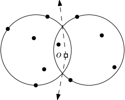
Figure 1: The restricted 2-center problem: two congruent disks of the smallest radius enclosing the points overlap.

The restricted 2-center problem can be solved by Sharir’s algorithm in $O(n\log^{9}n)$ time [13]. Eppstein gave a randomized algorithm which solves the restricted 2-center problem in $O(n\log n\log\log n)$ expected time [6].

In 1999, Chan [2] made an improvement to Eppstein’s algorithm by showing that the restricted 2-center problem can be solved in $O(n\log n)$ time with high probability. He also presented a deterministic $O(n\log^{2}n\log^{2}\log n)$-time algorithm for the restricted 2-center problem by using parametric search. Together with the $O(n\log^{2}n)$-time algorithm for the well-separated case by Eppstein [6], the planar 2-center problem is solved in $O(n\log^{2}n)$ time with high probability, or in $O(n\log^{2}n\log^{2}\log n)$ deterministic time.

Since then there was no improvement over 20 years until Wang [15] very recently gave an $O(n\log n\log\log n)$-time deterministic algorithm for the restricted 2-center problem, improving on Chan’s method by a $\log n\log\log n$ factor. Combining Eppstein’s $O(n\log^{2}n)$-time algorithm for the well-separated case, the planar 2-center problem can be solved in $O(n\log^{2}n)$ time deterministically. The improvement is from a new $O(n)$-time sequential decision algorithm, precomputing the intersections of disks that are frequently used in the parallel algorithms, and a dynamic data structure called the circular hull that maintains the intersection of the disks containing a fixed set of points. See the right figure in Figure 2.

Eppstein showed that any deterministic algorithm for the two-center problem requires $\Omega(n\log n)$ time in the algebraic decision tree model of computation by reduction from max gap problem [6]. So there is some gap between the best known running time and the lower bound.

1.1 Our results

We consider the restricted 2-center problem and show that the problem can be solved in $O(n\log n)$ time deterministically. This improves the previous best $O(n\log n\log\log n)$ bound by Wang by a $\log\log n$ factor.

Our algorithm follows the framework by Wang [15] (and thus by Chan [2]) and uses the $O(n)$-time sequential decision algorithm by Wang. But for the parallel algorithm, we use a different approach of running a decision algorithm in $O(\log n)$ parallel steps using $O(n)$ processors after $O(n\log n)$-time preprocessing.

By following Wang’s approach, our algorithm divides the points into a certain number of groups, computes for each group the common intersection of the disks centered at some points in the group and applies binary search on the intervals of indices independently. Wang used $O(\log n)$ processors to compute the intersections in $O(\log n\log\log n)$ time. In our algorithm, we increase the number of processors to $O(\log^{2}n)$ so that the time complexity to compute the intersections decreases to $O(\log n)$.

Another difference to the approach by Wang is that for each group, we additionally construct a data structure that determines the emptiness of intersections with respect to some common intersection. This can be done in $O(\log n)$ time using $O(\log^{6}n)$ processors. We use this data structure in binary search steps. It takes $O(\log^{3}\log n)$ time to determine if the common intersection is empty or not, which improves the $O(\log n)$-time result by Wang.

Thus our decision algorithm takes $O(\log n)$ time using $O(n)$ processors, after $O(n\log n)$-time preprocessing. We apply Cole’s parametric search technique [3] to compute $r^{*}$ in $O((T_{S}+Q)(T_{P}+\log Q))$ time, where $T_{S}=O(n)$ is sequential decision time, $T_{P}=O(\log n)$ is parallel decision time and $Q=O(n)$ is number of processor for parallel decision algorithm. Thus the optimal radius $r^{*}$ for the restricted 2-center can be computed in $O(n\log n)$ time.

We also consider the 2-center problem for the special case that the input points are in convex position. Kim and Shin [11] considered a variant of this problem for convex polygons: Given a convex polygon, find two smallest congruent disks whose union contains the polygon. They presented an $O(n\log^{2}n)$-time algorithm for a convex $n$-gon and claimed that the 2-center problem for $n$ points in convex position can be solved similarly in the same time. But Tan [14] pointed out a mistake in the time analysis, and presented an $O(n\log^{2}n)$-time algorithm for the problem. But Wang [15] showed a counterexample to the algorithm by Tan, and gave an $O(n\log n\log\log n)$-time algorithm for this problem [15].

We present a deterministic $O(n\log n)$-time algorithm that computes the optimal 2-center for the points in convex position. We first spend $O(n\log n)$ time to find a point contained in the overlap of the two optimal disks and a line separating the input points into two subsets. Then we apply our algorithm for the restricted 2-center problem to find an optimal pair of disks covering the input points.

2 Preliminaries

For a point set $X$ in the plane, we denote by $I_{r}(X)$ the common intersection of the disks with radius $r$, one centered at each point in $X$. The circular hull $\alpha_{r}(X)$ of $X$ is the common intersection of all disks of radius $r$ containing $X$. See Figure 2 for an illustration.

Figure 2: Five points (black dots) in $X$. (a) The intersection $I_{r}(X)$. (b) The circular hull $\alpha_{r}(X)$.

Clearly, both $I_{r}(X)$ and $\alpha_{r}(X)$ are convex. Observe that $I_{r}(X)$ and $\alpha_{r}(X)$ are dual to each other in the sense that every arc of $I_{r}(X)$ is on the circle of radius $r$ centered at a vertex of $\alpha_{r}(X)$ and every arc of $\alpha_{r}(X)$ is on the circle of radius $r$ centered at a vertex of $I_{r}(X)$. We may simply use $I(X)$ and $\alpha(X)$ instead of $I_{r}(X)$ and $\alpha_{r}(X)$ if they are understood from the context.

For a compact set $C$ in the plane, we use $\partial C$ to denote the boundary of $C$. For any two points $p,q\in\partial C$, we use $C[p,q]$ to denote the part of the boundary of $C$ from $p$ to $q$ in counterclockwise order.

Let $S$ be a set of $n$ points in the plane, and let $D^{*}_{1}$ and $D^{*}_{2}$ be the two congruent disks of an optimal solution for the restricted 2-center problem on $S$. We can find in $O(n)$ time a constant number of points such that at least one of them lies in $D^{*}_{1}\cap D^{*}_{2}$. We use $o$ to denote a point in $D^{*}_{1}\cap D^{*}_{2}$.

Without loss of generality, we assume that $o$ is at the origin of the coordinate system. Let $S^{+}$ denote the set of points of $S$ that lie above the $x$-axis, and $S^{-}$ denote $S\setminus S^{+}$. For ease of description, we assume that both $S^{+}$ and $S^{-}$ have $n$ points. Let $s^{+}_{1},s^{+}_{2},\ldots,s^{+}_{n}$ be the points of $S^{+}$ sorted around $o$ in counterclockwise order and $s^{-}_{1},s^{-}_{2},\ldots,s^{-}_{n}$ be the points of $S^{-}$ sorted around $o$ in counterclockwise order such that they appear in order from $s^{+}_{1}$ to $s^{+}_{n}$ and then $s^{-}_{1}$ to $s^{-}_{n}$ around $o$ in counterclockwise order. For any $1\leqslant i\leqslant j\leqslant n$, let $S^{+}[i,j]=\{s^{+}_{i},s^{+}_{i+1},\ldots,s^{+}_{j}\}$ and $S^{-}[i,j]=\{s^{-}_{i},s^{-}_{i+1},\ldots,s^{-}_{j}\}$.

There are two rays $\mu_{1},\mu_{2}$ emanating from $o$ that separate the points of $S$ into two subsets, each covered by one optimal disk. See Figure 1. Since such two rays are always separated by the $x$-axis or the $y$-axis [2], we simply assume that $\mu_{1}$ goes upward and $\mu_{2}$ goes downward.

For two indices $i,j\in[0,n]$, let $A[i,j]$ denote the radius of the smallest disk enclosing $S^{+}[i+1,n]\cup S^{-}[1,j]$, and let $B[i,j]$ denote the radius of the smallest disk enclosing $S^{+}[1,i]\cup S^{-}[j+1,n]$. For convenience, we let $S^{+}[n+1,n]=S^{+}[1,0]=S^{-}[n+1,n]=S^{-}[1,0]=\emptyset$.

For two points $p$ and $q$ in the plane, we use $\overrightarrow{pq}$ to denote a ray emanating from $p$ going towards $q$.

3 Improved algorithm for the restricted 2-center problem

Our algorithm follows the framework by Wang [15] (and thus by Chan [2]), and uses the $O(n)$-time sequential decision algorithm (after $O(n\log n)$-time preprocessing) by Wang. But for the parallel algorithm, we use a different approach of running a decision algorithm in $O(\log n)$ parallel steps using $O(n)$ processors after $O(n\log n)$-time preprocessing.

Let $r_{ij}=\max(A[i,j],B[i,j])$ and $r^{*}_{i}=\min_{0\leqslant j\leqslant n}r_{ij}$. Then $r^{*}=\min_{0\leqslant i\leqslant n}r^{*}_{i}$, where $r^{*}$ is the optimal radius for the restricted 2-center problem on $S$. Let $R=(r_{ij})$ be the $n\times n$ matrix whose $(i,j)$-entry is $r_{ij}$. Let $j(i)=\arg_{j}\min r_{ij}$. Observe that $R$ is monotone by the definition of $r_{ij}$, that is, for any two indices $i_{1}>i_{2}$ we have $j(i_{1})\geqslant j(i_{2})$.

We search for $r^{*}$ among the entries in $R$. We can determine whether $r^{*}<r$ by checking if there is some $i$ with $r^{*}_{i}<r$. Observe that for a fixed $i$, $A[i,j]$ increases and $B[i,j]$ decreases as $j$ increases. Therefore, $r_{ij}$ decreases and then increases as $j$ increases. By this property we can apply binary search in determining for a given $r$ if $r^{*}_{i}<r$ or not. However, it takes too much time for our purpose to apply binary search directly on the entries of $R$. Instead, we restrict binary search to certain elements of $R$ using the monotone property of $R$, and construct a few data structures to speed up the decision procedure as follows.

The algorithm consists of three phases. In Phase 1, our algorithm constructs a data structure on $S$ such that given a query consisting of $r>0$ and an interval $[i,j]$ it returns $I_{r}(S^{+}[i,j])$ or $I_{r}(S^{-}[i,j])$. It also reduces the search space in $R$ by evaluating on $r_{ij}$ at every $(\log^{6}n)$-th $j$ values from $j=1$. This gives us a set of $O(n/\log^{6}n)$ disjoint submatrices of $R$ with height $\log^{6}n$. Then it divides each of these submatrices further such that its width is at most $\log^{6}n$. So there are $O(n/\log^{6}n)$ groups. See Figure 5. In Phase 2, given $r>0$, our algorithm constructs a data structure for each submatrix obtained from Phase 1 such that given two indices $i$ and $j$ with $r_{ij}$ in the submatrix it determines whether $I_{r}(S^{+}[i,n])\cap I_{r}(S^{-}[1,j])=\emptyset$ or not. In Phase 3, our algorithm applies binary search to find a radius smaller than $r$ among the elements in each submatrix using the intersection emptiness queries on the data structure in Phase 2.

3.1 Phase 1: Preprocessing

In Phase 1, we construct a data structure on $S$ and reduce the search space in $R$.

3.1.1 Data structure

In this section, $r$ is a certain radius such that $I_{r}(\cdot)$ and $I_{r^{*}}(\cdot)$ have the same combinatorial structure. We build a balanced BST(binary search tree) on $S$ as follows. Let $\mathcal{T}(S)$ denote a balanced BST on an ordered point set $S$. Each leaf node corresponds to an ordered point in $S$ in order, from left to right. Each nonleaf node corresponds to the points of $S$ corresponded to by the leaf nodes of the subtree rooted at the node. For a node $w$, let $S_{w}$ denote the set of points corresponding to $w$. See Figure 3(a).

Observe that any interval $[i,j]$ of points of $S$ can be presented by $O(\log n)$ nodes and they can be found in $O(\log n)$ time as a range can be represented by $O(\log n)$ subtrees in the 1-dimensional range tree on $S$. We call these nodes the canonical nodes of the interval in $\mathcal{T}(S)$. For instance, the internal node corresponding to $\{p_{1},p_{2}\}$ and the leaf node corresponding to $p_{3}$ are the canonical nodes of interval $[1,3]$ in Figure 3(a). At each nodes $w$ in $\mathcal{T}(S)$, we store $I_{r}(S_{w})$ as an additional information.

The boundary of $I_{r}(S_{w})$ is represented by a balanced binary search tree and stored at $w$. The balanced binary search trees for the nodes in $\mathcal{T}(S)$ are computed in bottom-up manner in $O(n\log n)$ total time. See Figure 3. Thus, $\mathcal{T}(S)$ can be constructed in $O(n\log n)$ time.

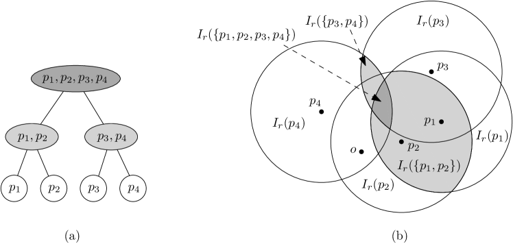
Figure 3: (a) The balanced binary search tree $\mathcal{T}(S)$ for $S=\{p_{1},p_{2},p_{3},p_{4}\}$. (b) The boundary of $I_{r}(S_{w})$ for a node $w$ in the tree in (a) is represented by a balanced binary search tree and stored at $w$.

The following two technical lemmas can be shown by lemmas in Wang’s paper [15] as $I_{r}(S_{w})$ is the dual of the circular hull $\alpha_{r}(S_{w})$.

Lemma 1 (Lemma $6$ in [15]).

$\mathcal{T}(S)$ can be constructed in $O(n\log n)$ time such that the combinatorial structure of $I_{r}(S_{w})$ is same as $I_{r^{*}}(S_{w})$ for any $w\in\mathcal{T}(S)$.

Lemma 2 (Lemma $5$ in [15]).

Let $L$ and $R$ be the point sets in the plane such that $L$ and $R$ are separated by a line and the arcs of $I_{r}(L)$ and $I_{r}(R)$ are stored in a data structure supporting binary search. One can do the following operation in $O(\log(|L|+|R|))$ time: determine whether $I_{r}(L)\cap I_{r}(R)=\emptyset$ or not; if $I_{r}(L)\cap I_{r}(R)\neq\emptyset$, either determine whether $I_{r}(L)\subseteq I_{r}(R)$ or $I_{r}(R)\subseteq I_{r}(L)$, or find the two intersection points of $\partial I_{r}(L)$ and $\partial I_{r}(R)$.

3.1.2 Speeding up intersection queries

Given a query range $[i,j]$, we can compute the common intersection $I(S^{+}[i,j])$ for points in $S^{+}[i,j]$ by computing the common intersection of $I(S_{w})$’s for all canonical nodes $w$ of $S^{+}[i,j]$ in $\mathcal{T}(S^{+})$ by Lemma 2, and by splitting and gluing the binary search trees stored in the canonical nodes. Wang showed a parallel algorithm for this process using $O(\log n)$ processors and running in $O(\log n\log\log n)$ time. Wang’s algorithm handles gluing two binary trees at a processor.

We can improve the query time for our purpose by using more processors, and by splitting and gluing multiple (more than two) binary trees simultaneously to compute the boundary arcs of common intersections using the order of the boundary arcs. Our algorithm computes the part of $\partial I_{i}$ that appears on the boundary of the common intersection. To compute the boundary part of $I_{i}$ efficiently, we represent the intersection of two regions in a number of intervals on its boundary.

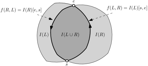
Figure 4: $I(L)\cap I(R)$ consists of two boundary parts, $f(L,R)$ and $f(R,L)$.

For a set of points in the plane, let $L$ and $R$ be the subsets of the points separated by a line. Then $\partial I(L)$ and $\partial I(R)$ intersect as most twice. Thus, we can represent $I(L)\cap I(R)$ by two boundary parts, one from $\partial I(L)$ and one from $\partial I(R)$, as follows. Let $f(L,R)$ and $f(R,L)$ denote the parts of $\partial I(L)$ and $\partial I(R)$, respectively, such that $f(L,R)$ and $f(R,L)$ together form the boundary of $I(L)\cap I(R)$. We can represent $f(L,R)$ by the two intersection points $\partial I(L)\cap\partial I(R)$ and the counterclockwise direction along $\partial I(L)$. For two intersection points $s,e$ of $\partial I(L)\cap\partial I(R)$, we use $f(L,R)=I(L)[s,e]$ if $s$ appears before $e$ on $\partial I(L)\cap\partial I(R)$ along $\partial I(L)$ in counterclockwise direction. See Figure 4.

For a family $\mathcal{W}$ of point sets, let $I(\mathcal{W})=I(\bigcup_{W\in\mathcal{W}}W)$ for ease of use. The boundary $\partial I(\mathcal{W})$ consists of $I(\mathcal{W})\cap\partial I(W)$ for each subset $W\in\mathcal{W}$. To compute $I(\mathcal{W})\cap\partial I(W)$, we need following lemma. We use $U^{+}(i,j)$ (and $U^{-}(i,j)$) to denote the set of the canonical nodes of range $[i,j]$ for $\mathcal{T}(S^{+})$ (and $\mathcal{T}(S^{-})$).

Lemma 3.

Let $X$ be a fixed point set and let $\mathcal{W}$ be a family of point sets. If we have $f(X,W)$ for every $W\in\mathcal{W}$ and a point $x\in I(X)$, there are at most $|\mathcal{W}|$ connected components of $I(\mathcal{W})\cap\partial I(X)$, each of which can be represented by a connected part of $\partial I(X)$, and we can compute them in $O(|\mathcal{W}|\log|\mathcal{W}|)$ time. If $X=S_{w}$ for a node $w\in U^{+}(i,j)$ and $\mathcal{W}=\{S_{w^{\prime}}\mid w^{\prime}\in U^{+}(i,j)\}$, there are at most two such connected components and we can compute them in $O(|\mathcal{W}|)$ time .

Proof.

For a set $W\in\mathcal{W}$, consider $f(X,W)=I(X)[s,e]$. For a point $x\in I(X)$, $I(X)[s,e]$ can be considered as an angle interval $[\theta_{s},\theta_{e}]$ with respect to $x$, where $\theta_{s}$ and $\theta_{e}$ are the angles of $\overrightarrow{xs}$ and $\overrightarrow{xe}$. (Note that the endpoints of $I(X)[s,e]$ can be represented as algebraic functions of $r$ with constant degree for $r$. For ease of description, we simply use the angles instead.)

By sorting the endpoints of the angle intervals, we can compute $\bigcap_{W\in\mathcal{W}}f(X,W)$, which is $I(\mathcal{W})\cap\partial I(X)$. However, there are only two such angle intervals if $X=S_{w}$ for a node $w\in U^{+}(i,j)$ and $\mathcal{W}=\{S_{w^{\prime}}\mid w^{\prime}\in U^{+}(i,j)\}$, and thus we can compute $I(\mathcal{W})\cap\partial I(X)$ in $O(|\mathcal{W}|)$ time as follows. Let $S_{w}=S^{+}[i^{\prime},j^{\prime}]$, then $\mathcal{W}$ can be partitioned into three subfamilies $\{S_{w}\},\mathcal{W}_{L}=U^{+}(j^{\prime}+1,j)$, and $\mathcal{W}_{R}=U^{+}(i,i^{\prime}-1)$. Observe that the subfamilies are separated by the two lines, both through the origin, one through $p_{j^{\prime}}$ and one through $p_{i^{\prime}}$. Let $A_{L}$ be the set of angle intervals from $f(X,W_{L})$ for $W_{L}\in\mathcal{W}_{L}$ and let $I_{L}$ be the common intersection of the angle intervals in $A_{L}$. The common intersection of the angle intervals of any subset of $A_{L}$ consists of at most one angle interval by Lemma 2, because any set of $\mathcal{W}_{L}$ is separated from $S_{w}$ by a line. Consider an angle interval $[\theta_{s},\theta_{e}]$ of $A_{L}$. Then the intersection of $[\theta_{s},\theta_{e}]$ with every other angle interval in $A_{L}$ is connected. Thus, we compute the common intersection $I_{L}$ of the angle intervals of $A_{L}$ within $[\theta_{s},\theta_{e}]$ in $O(|A_{L}|)$ time. For the set of angle intervals from $f(X,W_{R})$ for $W_{R}\in\mathcal{W}_{R}$, we can compute the common intersection of those intervals in a similar way. Thus there are at most two such connected components and we can compute them in $O(|\mathcal{W}|)$ time.    

In the following, we abuse $I(i,j)$ to denote $I(S^{+}[i,j])$ for any two indices $i,j$ satisfying $1\leqslant i\leqslant j\leqslant n$. To merge the boundaries we need to know their appearing order in boundary of common intersection.

Lemma 4.

The indices of the points corresponding to the arcs of $\partial I(i,j)$ are increasing and decreasing consecutively at most once while traversing along $\partial I(i,j)$.

Proof.

We use circular hulls $\alpha_{r}(\cdot)$ to prove the lemma. Since $I_{r}(\cdot)$ and $\alpha_{r}(\cdot)$ are dual to each other, the proof also holds for $I_{r}(\cdot)$. We simply use $\alpha(\cdot)$ to denote $\alpha_{r}(\cdot)$. For any two indices $i$ and $j$, we show that the indices of the vertices that appear on the boundary of $\alpha(S^{+}[i,j])$ are increasing and decreasing consecutively at most once.

Consider the case that $\alpha(S^{+}[i,j])$ does not contain $o$. Let $x_{1}$ and $x_{2}$ be the contact points of the right and left tangent lines to $\alpha(S^{+}[i,j])$ from $o$. For a point $p$ on the boundary of $\alpha(S^{+}[i,j])$, the angle between $\overrightarrow{op}$ and the $x$-axis is increasing while moving along the boundary of $\alpha(S^{+}[i,j])$ from $x_{1}$ to $x_{2}$ in counterclockwise order. Similarly, the angle between $\overrightarrow{op}$ and the $x$-axis is decreasing while moving along the boundary of $\alpha(S^{+}[i,j])$ from $x_{2}$ to $x_{1}$ in counterclockwise order. Thus, the indices of the vertices of the circular hull are increasing and decreasing at most once.

Now consider the case that $\alpha(S^{+}[i,j])$ contains $o$. By the definitions of $o$ and $S^{+}$, there is no vertex of $\alpha(S^{+}[i,j])$ lying below the $x$-axis. Thus, for a vertex $v$ of $\alpha(S^{+}[i,j])$, the angle between $\overrightarrow{ov}$ and the $x$-axis is increasing while moving along the boundary of $\alpha(S^{+}[i,j])$ from $p_{s}$ to $p_{t}$ in counterclockwise, where $s$ and $t$ are the smallest and largest indices of the vertices of $\alpha(S^{+}[i,j])$.

Since the order of the vertices on the boundary $\alpha(S^{+}[i,j])$ is the same as the order of the indices of points corresponding to the arcs of $\partial I(i,j)$, the lemma holds.    

We construct $\mathcal{T}(S^{+})$ (and $\mathcal{T}(S^{-})$) in $O(n\log n)$ time using Lemma 1. Now, we have basic lemmas on queries to $\mathcal{T}(S^{+})$ (and $\mathcal{T}(S^{-})$). Let $(r_{1},r_{2}]$ be the range of radius $r$ for which $I_{r}(S_{w})$ and $I_{r^{*}}(S_{w})$ have the same combinatorial structure for any $w\in\mathcal{T}(S^{+})$.

Lemma 5.

Once $\mathcal{T}(S^{+})$ is constructed, we can process the following queries in $O(\log n)$ time using $O(\log^{2}n)$ processors: given $r\in(r_{1},r_{2}]$ and any pair $(i,j)$ of indices, determine whether $I(i,j)=\emptyset$ or not, and if $I(i,j)\neq\emptyset$, return the root of a balanced binary search tree representing $I(i,j)$.

Proof.

Observe that $\partial I(i,j)$ consists of parts of $\partial I(S_{w})$ for all canonical nodes $w\in U^{+}(i,j)$. For a fixed $w\in U^{+}(i,j)$, we compute $I(i,j)\cap\partial I(S_{w})$ by taking $f(S_{w},S_{w^{\prime}})$ for every canonical node $w^{\prime}\in U^{+}(i,j)$ and applying Lemma 3. For a fixed $w\in U^{+}(i,j)$, we can compute $f(S_{w},S_{w^{\prime}})$ for every $w^{\prime}\in U^{+}(i,j)$ in $O(\log n)$ parallel steps using $O(\log n)$ processors. By Lemma 3, there are at most two boundary parts representing $I(i,j)\cap\partial I(S_{w})$, and we can find them in $O(\log n)$ time using one processor.

For a part $I(S_{w})[s,e]$, we construct a binary search tree for $I(S_{w})[s,e]$ using $I(S_{w})$ stored at $w\in\mathcal{T}(S^{+})$ and the path copying [4] in $O(\log n)$ time. Since there are $O(\log n)$ nodes in $U^{+}(i,j)$, we can find $O(\log n)$ binary search trees, at most two for each node, in $O(\log n)$ parallel steps using $O(\log^{2}n)$ processors. Observe that the binary search trees for a point set $S_{w}$ represents $I(i,j)\cap\partial I(S_{w})$.

Then we merge all these binary search trees into a binary search tree representing $\partial I(i,j)$. By Lemma 4, the indices of the points in $S^{+}[i,j]$ corresponding to the arcs of $\partial I(i,j)$ are increasing and then decreasing consecutively at most once while traversing along $\partial I(i,j)$. For any two distinct canonical nodes $w,w^{\prime}$ of $U^{+}(i,j)$, we use $w<w^{\prime}$ if the indices of the points in $S_{w}$ are smaller than the indices of the points in $S_{w^{\prime}}$. Since the canonical nodes of $U^{+}(i,j)$ can be ordered by their corresponding point sets, the binary trees can also be ordered accordingly, by following the orders of their corresponding canonical nodes. Each canonical node $w$ has at most two parts of $I(i,j)\cap\partial I(S_{w})$, and the order between the binary search trees on the parts is decided by the order of their corresponding canonical nodes in $\mathcal{T}(S^{+})$.

Following this order, we merge the $O(\log n)$ binary search trees in $O(\log n)$ time. Recall that there are at most two binary search trees $T,T^{\prime}$ for each node $U^{+}(i,j)$, which are at the same position in the order. Thus, the merge process is done in two passes, one in the order and one in reverse of the order, and $T$ is merged as a boundary part of $I(i,j)$ in one pass and $T^{\prime}$ is merged as a boundary part of $I(i,j)$ the other pass. By repeating this process on the binary search trees in order, we can construct $\partial I(i,j)$. Finally we can return the root of the merged binary search tree representing $I(i,j)$ in $O(\log n)$ time using $O(\log^{2}n)$ processors.    

3.1.3 Reducing the search space to submatrices

Our algorithm reduces the set of candidates for $r^{*}$ from the elements in the $n\times n$ matrix $R=(r_{ij}$) to the elements in $O(n/\log^{6}n)$ disjoint submatrices of size $\log^{6}n\times\log^{6}n$ in $R$. This is done by evaluating on $r_{ij}$ at every $\log^{6}n$-th $j$ values from $j=1$, which results in a set of $O(n/\log^{6}n)$ disjoint submatrices of of $R$ with height $\log^{6}n$. Then we divide each of these submatrices further such that its width is at most $\log^{6}n$. See Figure 5.

Precisely, let $m=\lfloor n/\log^{6}n\rfloor$, $j_{t}=t\times\lfloor n/m\rfloor$ for $t=0,1,\ldots,m$. For each $t\in[0,m]$, let $i_{t}$ be the largest index in $[0,n]$ satisfying $A[i_{t},j_{t}]\geqslant B[i_{t},j_{t}]$. Observe that $i_{0}\leqslant i_{1}\leqslant\ldots\leqslant i_{m}$. Each $i_{t}$ can be found in $O(\log^{7}n)$ time after $O(n\log n)$-time preprocessing. Since there are $O(m)$ such $i_{t}$’s, we can compute them in $O(n\log n)$ time [2].

The algorithm determines whether $r_{i}^{*}\leqslant r$ or not, for all $i=0,1,\ldots,n$, as follows. For each $i$, let $t$ be an index in $[0,m-1]$ satisfying $i_{t}<i\leqslant i_{t+1}$. If $A[i,j_{t}]>r$, then the algorithm returns $r^{*}_{i}>r$. Otherwise, it finds the largest index $j\in[j_{t},j_{t+1}]$ satisfying $A[i,j]\leqslant r$, and returns $r_{i}^{*}\leqslant r$ if and only if $B[i,j]\leqslant r$. See Algorithm 2 of [15] and Theorem 4.2 of [2].

Our algorithm divides the indices $i$ from 0 to $n$ into at most $2m$ groups. For each $t=0,1,\ldots,m-1$, if $i_{t+1}-i_{t}\leqslant\log^{6}n$ , the algorithm forms a group of at most $\log^{6}n$ indices. Otherwise it forms a group for every consecutive $\log^{6}n$ indices up to $i_{t+1}$. Then there are at most $2m$ groups. Each group $G=[a,b]$ is contained in one of $[i_{t},i_{t+1}]$. We identify group $G$ as $G(a,b,t)$. See Figure 5.

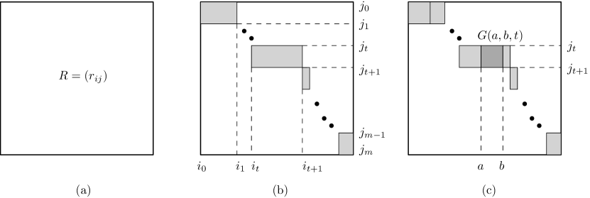
Figure 5: (a) Matrix $R=(r_{ij})$. (b) Reducing the search space into $O(n/\log^{6}n)$ submatrices of height $\log^{6}n$ using the monotone property, at every $(\log^{6}n)$-th entries of index $j$. (c) Dividing each submatrix further into one with width at most $\log^{6}n$. A submatrix (a group of indices) $G(a,b,t)$ represents the index ranges of $i$ from $a$ to $b$ and of $j$ from $j_{t}$ to $j_{t+1}$.

For each group $G(a,b,t)$, we construct $\mathcal{T}(S^{+}[a,b])$ and $\mathcal{T}(S^{-}[j_{t},j_{t+1}])$, which will be used to construct a data structure for determining the emptiness of intersections. This can be done for all groups in $O(n\log n)$ time in total.

3.2 Phase 2 - Group information

Given a value $r>0$, we determine if $A[i,j]\leqslant r$ for a group $G(a,b,t)$ with $a\leqslant i\leqslant b$ and $j_{t}\leqslant j\leqslant j_{t+1}$. Observe that the points of $S^{+}[b,n]$ and the points of $S^{-}[1,j_{t}]$ are used commonly in the process. See Figure 6.

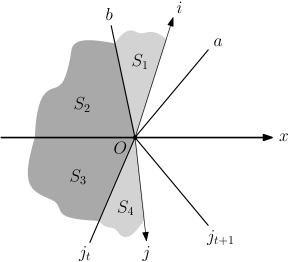
Figure 6: To determine if $A[i,j]\leqslant r$ for a $G(a,b,t)$ with $a\leqslant i\leqslant b$, $j_{t}\leqslant j\leqslant j_{t+1}$, we use four subsets $S_{1}=S^{+}[i,b],S_{2}=S^{+}[b,n],S_{3}=S^{-}[1,j_{t}],$ and $S_{4}=S^{-}[j_{t},j]$. Observe that $b,j_{t}$ and $n$ are constant, and $|b-a|,|j_{t+1}-j_{t}|\leqslant\log^{6}n$.

The decision algorithm consists of computing group information and binary search. We simply use $I(\cdot)$ to denote $I_{r}(\cdot)$. For for each group $G(a,b,t)$, the algorithm computes $I(S^{+}[b,n])$ and $I(S^{-}[1,j_{t}])$. And then it constructs a data structure such that given query indices $i$ and $j$ with $a\leqslant i\leqslant b$ and $j_{t}\leqslant j\leqslant j_{t+1}$, it determines if $I(S^{+}[i,n])\cap I(S^{-}[1,j])=\emptyset$ or not using $I(S^{+}[b,n])$ and $I(S^{-}[1,j_{t}])$. In the binary search, we determine $A[i,j]\leqslant r$ or not (and $B[i,j]\leqslant r$ or not) using emptiness queries on this data structure.

For an ordered point set $L$ and any point set $R$ separated by a line in the plane, let $\mathcal{D}(L,R)$ be a balanced BST on the ordered set $L$ with respect to $R$ constructed from $\mathcal{T}(L)$ such that for each node $w$ in $\mathcal{T}(L)$, we store $f(S_{w},R)$ and $f(R,S_{w})$ instead of $I(S_{w})$. This data structure will be used to determine if $I(L^{\prime}\cup R)=\emptyset$ or not for any interval $L^{\prime}\subseteq L$.

Lemma 6.

$\mathcal{D}(L,R)$ can be constructed in $O(\log(|L|+|R|))$ time using $O(|L|)$ processors once we have $\mathcal{T}(L)$ and $I(R)$, where $L$ and $R$ are line separated continuous ordered point set.

Proof.

First we assign a processor to a node $w\in\mathcal{T}(L)$. Since there are $O(|L|)$ nodes in $\mathcal{T}(L)$ and the tree depth is $O(\log|L|)$, we can assign $O(|L|)$ processors in $O(\log|L|)$ time. For each nodes $w$, we compute $f(S_{w},R)$ and $f(R,S_{w})$. This can be done using $I(S_{w}),I(R),$ and Lemma 2 in $O(\log(|S_{w}|+|R|)$ time. Since $S_{w}\subseteq L$, $\mathcal{D}(L,R)$ can be constructed in $O(\log(|L|+|R|))$ time using $O(|L|)$ processors.    

We will apply binary search for each index $i$. Each index $i$ is contained in one of the $2m$ groups. Each group $G(a,b,t)$ consists of continuous $O(\log^{6}n)$ indices $\{a,a+1,\ldots,a+b\}$. For an index $i\in G(a,b,t)$, the decision on $A[i,j]\leqslant r$ is equivalent to the decision on $I_{ij}=\bigcap_{k=1}^{4}I(S_{k})\neq\emptyset$, where $S_{1}=S^{+}[i,b],S_{2}=S^{+}[b,n],S_{3}=S^{-}[1,j_{t}],$ and $S_{4}=S^{-}[j_{t},j]$. The emptiness of $I_{ij}$ is equivalent to the emptiness of $\partial I_{ij}$. Since $\partial I_{ij}$ consists of boundary parts of $I(S_{k})$ for each $k=1,\ldots,4$, the emptiness of $I_{ij}$ is equivalent to the emptiness of $I_{ij}\cap\partial I(S_{k})$ for every $k=1,\ldots,4$.

Now we list all the information we need in computing $\partial I(S_{1})$ and $I_{ij}\cap\partial I(S_{2})$. Observe that $I_{ij}\cap\partial I(S_{1})$ consists of parts of the boundaries $I_{ij}\cap\partial I(S_{w})$ for the canonical nodes $w\in U^{+}(i,b)$. To compute $I_{ij}\cap\partial I(S_{w})$ for a node $w\in U^{+}(i,b)$ using Lemma 3, we need $f(S_{w},S_{1})$, $f(S_{w},S_{2})$, $f(S_{w},S_{3})$ and $f(S_{w},S_{4})$. We compute $f(S_{w},S_{2})$ and $f(S_{w},S_{3})$ in this Phase. Then we compute $f(S_{w},S_{1})$ and $f(S_{w},S_{4})$ in Phase 3.

To compute $I_{ij}\cap\partial I(S_{2})$ using lemma 3, we need $f(S_{2},S_{3})$ and $f(S_{2},S_{w})$ for every node $w\in U^{+}(i,b)\cup U^{-}(j_{t},j)$. We compute them all in this Phase. We can compute $I_{ij}\cap\partial I(S_{4})$ and $I_{ij}\cap\partial I(S_{3})$ in a similar way.

To cover the query range, we need to compute $f(S_{w},S_{2})$, $f(S_{w},S_{3})$, $f(S_{2},S_{w})$ and $f(S_{3},S_{w})$ for every $w\in\mathcal{T}(S^{+}[a,b])\cup\mathcal{T}(S^{-}[j_{t},j_{t+1}])$ because $i\in[a,b]$ and $j\in[j_{t},j_{t+1}]$ while applying the binary search on the group.

We compute the followings for each group $G(a,b,t)$ in this phase.

1. $I(S_{2})$ and $I(S_{3})$.

2. $f(S_{2},S_{3})$ and $f(S_{3},S_{2})$.

3. $\mathcal{D}(S^{+}[a,b],S_{2})$, $\mathcal{D}(S^{+}[a,b],S_{3})$, $\mathcal{D}(S^{-}[j_{t},j_{t+1}],S_{2})$ and $\mathcal{D}(S^{-}[j_{t},j_{t+1}],S_{3})$.

Part 1 can be done in $O(\log n)$ time using $O(\log^{2}n)$ processors by Lemma 5. Part 2 can be done in $O(\log n)$ time by Lemma 2. Part 3 can be done $O(\log n)$ time using $O(\log^{6}n)$ processors by Lemma 6. Since there are $2m=O(n/\log^{6}n)$ such groups, the three parts can be done $O(\log n)$ time with $O(n)$ processors in total.

3.3 Phase 3 - Binary search

For an index $i\in G(a,b,t)$, we apply binary search over range $j\in[j_{t},j_{t+1}]$. Since $|j_{t+1}-j_{t}|=O(\log^{6}n)$, our algorithm performs $O(\log\log n)$ steps of binary search to determine whether $r_{i}^{*}\leqslant r$ or not.

To determine $I_{ij}\neq\emptyset$, we determine $I_{ij}\cap\partial I(S_{1})\neq\emptyset$, $I_{ij}\cap\partial I(S_{2})\neq\emptyset$, $I_{ij}\cap\partial I(S_{3})\neq\emptyset$, or $I_{ij}\cap\partial I(S_{4})\neq\emptyset$. To determine $I_{ij}\cap\partial I(S_{1})\neq\emptyset$, we determine $I_{ij}\cap\partial I(S_{w})\neq\emptyset$ for every canonical node $w\in U^{+}(i,b)$. To determine $I_{ij}\cap\partial I(S_{w})\neq\emptyset$ by Lemma 3, we compute $f(S_{w},S_{2})$, $f(S_{w},S_{3}),$ and $f(S_{w},S_{w^{\prime}})$ for all $w^{\prime}\in U^{+}(i,b)\cup U^{-}(j_{t},j)$, because the union of the intersections for $S_{2}$, $S_{3}$ and all $S_{w^{\prime}}$ is $I_{ij}$. We can compute $f(S_{w},S_{2})$ and $f(S_{w},S_{3})$ in $\mathcal{D}(S^{+}[a,b],S_{2})$ and $\mathcal{D}(S^{+}[a,b],S_{3})$, respectively, at the corresponding nodes $w$. We can compute $f(S_{w},S_{w^{\prime}})$ using $I(S_{w})$ and $I(S_{w^{\prime}})$, and the intersections $I(S_{w})$ and $I(S_{w^{\prime}})$ can be found in $\mathcal{T}(S^{+}[a,b])$ or $\mathcal{T}(S^{-}[j_{t},j_{t+1}])$. Since $|S_{w}|=O(\log^{6}n)$ and $|S_{w^{\prime}}|=O(\log^{6}n)$, it takes $O(\log\log n)$ time to compute $f(S_{w},S_{w^{\prime}})$ for fixed $w$ and $w^{\prime}$ by Lemma 3. Since $|U^{+}(i,b)\cup U^{-}(j_{t},j)|=O(\log\log n)$, it takes $O(\log^{2}\log n)$ time to compute $f(S_{w},S_{w^{\prime}})$ for all $w^{\prime}\in|U^{+}(i,b)\cup U^{-}(j_{t},j)|$. Thus we can determine $I_{ij}\cap\partial I(S_{w})\neq\emptyset$ in $O(\log^{2}\log n)$ time. Since $|U^{+}(i,b)|=O(\log\log n)$, $I_{ij}\cap\partial I(S_{1})$ can be determined $O(\log^{3}\log n)$ time with one processor.

To determine $I_{ij}\cap\partial I(S_{2})\neq\emptyset$, we need $f(S_{2},S_{3})$ and $f(S_{2},S_{w})$ for all $w\in U^{+}(i,b)\cup U^{-}(j_{t},j)$. We already have $f(S_{2},S_{3})$ and $f(S_{2},S_{w})$ can be computed from $\mathcal{D}(S^{+}[a,b],S_{2})$ and $\mathcal{D}(S^{-}[j_{t},j_{t+1}],S_{2})$ in $O(\log\log n)$ time. So we can determine $I_{ij}\cap\partial I(S_{2})\neq\emptyset$ in $O(\log\log n\log\log\log n)$ time with one processor.

Therefore, for a fixed $i$ and a given $j$, we can determine whether $I_{ij}$ is empty or not in $O(\log^{3}\log n)$ time. Remind that the search range for an index is $O(\log^{6}n)$. There are $O(\log\log n)$ steps of binary search and there are $n+1$ indices for $i$. The decision step can be done in $O(\log^{4}\log n)$ time using $O(n)$ processors.

Theorem 7.

The decision problem for the restricted 2-center problem can be solved in $O(\log n)$ time using $O(n)$ processors after $O(n\log n)$-time preprocessing.

Theorem 8.

The restricted 2-center problem can be solved in $O(n\log n)$ time.

Proof.

We use Cole’s parametric search technique [3] to compute the optimal radius $r^{*}$. To apply the technique, the parallel algorithm must satisfy a bounded fan-in/bounded fan-out requirement. Instead of analyzing the parallel algorithm directly, we divide the algorithm to a constant number of parts such that each part satisfies a bounded fan-in/bounded fan-out.

Our parallel decision algorithm computes some information for each group and applies binary search on indices. In the group information phase, we compute $I(S_{2})$ by computing $I(S_{2})\cap\partial I(S_{w})$ for every $w\in U^{+}(b,n)$ and merging them. Each $I(S_{2})\cap\partial I(S_{w})$ is computed by computing $f(S_{w},S_{w^{\prime}})$ for every $w^{\prime}\in U^{+}(b,n)$ and merging them. Thus, a processor activates at most one processor, and the fan-out is bounded. We also compute $f(S_{2},S_{3})$ for each group independently by a processor, and thus the fan-in and fan-out are bounded. We assign processors for all nodes $w$ without knowing the decision parameter $r$ in advance. Then each processor computes $f(S_{2},S_{w})$ and $f(S_{w},S_{2})$ for a node $w$ independently, and thus the fan-in and fan-out are bounded. In the binary search phase, each binary search for an index is performed by a processor independently, and thus the fan-in and fan-out are bounded.

Therefore, our parallel algorithm consists of a constant number of fan-in or fan-out bounded networks. Thus we can apply Cole’s parametric search technique to compute $r^{*}$ in $O((T_{S}+Q)(T_{P}+\log Q))$ time, where $T_{S}$ is the sequential decision time, $T_{P}$ is the parallel decision time and $Q$ is the number of processors for parallel decision algorithm. Since we have $T_{S}=O(n)$, $T_{P}=O(\log n)$ and $Q=O(n)$, $r^{*}$ can be computed in $O(n\log n)$ time.    

4 Optimal 2-center for points in convex position

In this section, we consider the 2-center problem for points in convex position. Wang gave an $O(n\log n\log\log n)$-time algorithm for this problem. Let $S$ be a point set consisting of $n$ points in convex position in the plane. We denote by $\mathsf{CH}(S)$ the convex hull of $S$. It is known that there is an optimal solution $(D_{1}^{*},D_{2}^{*})$ such that $D_{1}^{*}$ covers a set of consecutive vertices (points of $S$) along $\partial\mathsf{CH}(S)$ and $D_{2}^{*}$ covers the remaining points of $S$ [11]. Since the points are in convex position, for any point $q$ contained in $\mathsf{CH}(S)$, the points of $S$ appears in the same order around $q$.

Let $\mu_{1}$ and $\mu_{2}$ be the two rays from $o$ that separate the point set $S$ into two subsets, one covered by $D_{1}^{*}$ and the other covered by $D_{2}^{*}$. We need to find a line $\ell$ that separates $\mu_{1}$ and $\mu_{2}$. The line $\ell$ partitions the points of $S$ to $S^{+}$ and $S^{-}$. Then $o$ can be any point in $\ell$.

Wang gave an algorithm that finds the optimal two disks or the line $\ell$ in $O(n\log n)$ time [15]. The algorithm first sorts the points of $S$ along the boundary of $\mathsf{CH}(S)$ and pick any point $p_{1}\in S$. Then it finds $p^{*}\in S$ such that the two congruent smallest disks $(D_{1},D_{2})$ with $D_{1}$ covering $\mathsf{CH}(S)[p_{1},p^{*}]$ and $D_{2}$ covering $S\setminus\mathsf{CH}(S)[p_{1},p^{*}]$ have the minimum radius over all $p\in S$. The radius of $D_{1}$ covering $\mathsf{CH}(S)[p_{1},p_{j}]$ does not decrease while $p_{j}$ moves along the boundary of $\mathsf{CH}(S)$. Similarly, $D_{2}$ has this property. In each step of binary search, we compute $D_{1}$ and $D_{2}$ in $O(n)$ time. Thus, the algorithm can find $p^{*}$ in $O(n\log n)$ time using binary search. If $\mu_{1}$ passes through $p_{1}$, we already have the minimum radius. Otherwise, $\mu_{1}$ or $\mu_{2}$ passes through $p^{*}$ or one of its two neighboring point along $\mathsf{CH}(S)$, or $\mu_{1}$ crosses $\mathsf{CH}(S)[p_{1},p^{*}]$ and $\mu_{2}$ crosses $\mathsf{CH}(S)[p^{*},p_{1}]$. So we can find the optimal disks or the line $\ell$ that separates $\mu_{1}$ and $\mu_{2}$ in $O(n\log n)$ time.

Therefore, we can apply our algorithm in Section 3 to the points in convex position. From this, we improve the running time by a $\log\log n$ factor over the $O(n\log n\log\log n)$-time algorithm by Wang.

Theorem 9.

The 2-center problem for $n$ points in convex position in the plane can be solved in $O(n\log n)$ time.

5 Conclusions

We presented a deterministic $O(n\log n)$-time algorithm for the case that the centers of the two optimal disks are close together, that is, the overlap of the two optimal disks is a constant fraction of the disk area. Now for the planar 2-center problem, the bottleneck of the time bound is the case that the two optimal disks are disjoint, and Eppstein’s $O(n\log^{2}n)$-time algorithm is best for the case. Thus, the time for the planar 2-center problem still remains to be $O(n\log^{2}n)$ due to the well-separated case.

We also presented a deterministic $O(n\log n)$-time algorithm for $n$ points in convex position in the plane. This closes the long-standing question for the convex-position case.

References

- [1] Pankaj K. Agarwal and Micha Sharir. Planar geometric location problems. Algorithmica, 11(2):185–195, Feb 1994.
- [2] Timothy M. Chan. More planar two-center algorithms. Computational Geometry, 13(3):189–198, 1999.
- [3] Richard Cole. Slowing down sorting networks to obtain faster sorting algorithms. Journal of the ACM, 34(1):200–208, 1987.
- [4] James R Driscoll, Neil Sarnak, Daniel D Sleator, and Robert Endre Tarjan. Making data structures persistent. Journal of Computer and System Sciences, 38(1):86–124, 1989.
- [5] David Eppstein. Dynamic three-dimensional linear programming. ORSA Journal on Computing, 4(4):360–368, 1992.
- [6] David Eppstein. Faster construction of planar two-centers. In Proceedings of the 8th Annual ACM-SIAM Symposium on Discrete Algorithms (SODA 1997), pages 131–138, 1997.
- [7] John Hershberger. A faster algorithm for the two-center decision problem. Information Processing Letters, 47(1):23–29, 1993.
- [8] John Hershberger and Subhash Suri. Off-line maintenance of planar configurations. Journal of Algorithms, 21(3):453–475, 1996.
- [9] Jerzy W. Jaromczyk and Miroslaw Kowaluk. An efficient algorithm for the euclidean two-center problem. In Proceedings of the 10th Annual Symposium on Computational Geometry (SoCG 1994), pages 303–311, 1994.
- [10] Matthew J. Katz and Micha Sharir. An expander-based approach to geometric optimization. In Proceedings of the 9th Annual Symposium on Computational Geometry (SoCG 1993), pages 198–207, 1993.
- [11] Sung Kwon Kim and Chan-Su Shin. Efficient algorithms for two-center problems for a convex polygon. In Proceedings of the 6th International Computing and Combinatorics Conference (COCOON 2000), pages 299–309, 2000.
- [12] Nimrod Megiddo. Applying parallel computation algorithms in the design of serial algorithms. Journal of the ACM, 30(4):852–865, 1983.
- [13] M. Sharir. A near-linear algorithm for the planar 2-center problem. Discrete & Computational Geometry, 18(2):125–134, Sep 1997.
- [14] Xuehou Tan and Bo Jiang. Simple algorithms for the planar 2-center problem. In Proceedings of the 23rd International Computing and Combinatorics Conference (COCOON 2017), pages 481–491, 2017.
- [15] Haitao Wang. On the planar two-center problem and circular hulls. In Proceedings of the 36th International Symposium on Computational Geometry (SoCG 2020), pages 68:1–68:14, 2020.