Cell-Free Massive MIMO with Nonorthogonal Pilots for Internet of Things

Abstract

We consider Internet of Things (IoT) organized on the principles of cell-free massive MIMO. Since the number of things is very large, orthogonal pilots cannot be assigned to all of them even if the things are stationary. This results in an unavoidable pilot contamination problem, worsened by the fact that, for IoT, since the things are operating at very low transmit power. To mitigate this problem and achieve a high throughput, we use cell-free systems with optimal linear minimum mean squared error (LMMSE) channel estimation, while traditionally simple suboptimal estimators have been used in such systems. We further derive the analytical uplink and downlink signal-to-interference-plus-noise ratio (SINR) expressions for this scenario, which depends only on large scale fading coefficients. This allows us to design new power control algorithms that require only infrequent transmit power adaptation. Simulation results show a 40% improvement in uplink and downlink throughputs and 95% in energy efficiency over existing cell-free wireless systems and at least a three-fold uplink improvement over known IoT systems based on small-cell systems.

I Introduction

Internet of Things (IoT) represents an entirely new challenge to the wireless physical layer. In an IoT connectivity scenario, it is required to connect a large number, e.g., ten thousand or more, of users (things) of which only a small fraction is active simultaneously. (In what follows we will use “users” and “things” interchangeably when we talk about IoT.) Challenges that are inherent to IoT include: scale (the number of users is significantly greater than in cellular wireless), low power requirements for things (things are anticipated either to use energy harvesting or infrequently replaced batteries), emphasis on the uplink, typically low and/or sporadic data outputs from each thing, and possibly ultra-low latency requirements. Wireless massive multiple-input multiple-output (MIMO) systems look to be one of the best candidates for resolving the above challenges.

A number of works exist on the use of massive MIMO for massive connectivity in IoT. In [1] and [2], the authors provide a framework for user activity detection and channel estimation with a cellular base station (BS) equipped with a large number of antennas, and characterize the achievable uplink rate. The user activity detection is based on assigning a unique pilot to each user, which serves as the user identifier. These pilots then are used as columns of a sensing matrix. Active users synchronously send their pilots and a base station receives a linear combination of the those pilots. Next the base station runs a compressive sensing detection algorithm for the sensing matrix and identifies the pilots that occur as terms in the linear combination. These pilots, in their turn, reveals the active users.

Massive MIMO for IoT connectivity in the context of cyber-physical systems (CPS) is considered in [3], and orthogonal pilot reuse to simultaneously support a large number of active industrial IoT devices is studied in [4]. However, these works consider a centralized massive MIMO architecture where all the service antennas are collocated. The cell-free architecture assumes that access points (APs) are distributed over a wide area and that they are connected via a backhaul to a central processing unit (CPU). The coherent processing across APs provided by this architecture enables simple signal processing and power control. Although the low backhaul requirement of centralized MIMO is advantageous, the cell-free architecture is more suitable for IoT since it offers a greater coverage area.

In [5] and [6], achievable rates and power control algorithms for cell-free massive MIMO with a suboptimal channel estimation are studied. This estimation is optimal only if orthogonal pilots are reused among the users. One of the reasons for choosing this suboptimal channel estimation was that it was a common understanding that the linear minimum mean square error (LMMSE) channel estimation allows estimation of the user signal-to-interference-plus-noise ratio (SINR) only as a function of instantaneous channel state information (CSI), i.e., small scale channel coefficients. At the same time it is very desirable to get SINR estimates that depend only on large scale channel fading coefficients, which do not depend on orthogonal frequency-division multiplexing (OFDM) tone index and change about 40 times slower then small scale fading coefficients. Such expressions greatly reduce the complexity of power control and simplify the analysis of the system performance. In this work we show that this common understanding was a misconception, and derive uplink and downlink SINR expressions for the case of LMMSE channel estimation that are functions of only large scale fading coefficients, transmit power coefficients, and the used pilots. Our simulation results demonstrate that LMMSE channel estimation allows obtaining an additional $40\%$ performance gain in terms of data transmission rates compared with suboptimal channel estimation used in [5] and [6]. We next propose efficient power control algorithms. In the uplink, power control is performed by considering two criteria – the max-min SINR criterion and a target SINR criterion. In the latter, we try to ensure that each user attains a pre-defined SINR threshold. In the downlink, the power control optimization problem is formulated as a second-order cone program (SOCP) that can be solved efficiently. We also compare our systems with small-cell systems, which have been suggested as promising technology for future wireless systems [7, 8]. In a typical small-cell system, the APs are uniformly distributed in the coverage area and each user is served by a dedicated AP. Since the APs operate independently, the average data rate in a small-cell system is lower than in a cell-free system. We apply our power control algorithms to the system in [5] under correlated and uncorrelated shadow fading channels and show a significant gain in uplink and downlink throughputs over results obtained in [5], and over conventional small-cell systems.

In section II, we describe the cell-free massive MIMO system model, channel estimation, and the uplink and downlink transmissions. In section III, the uplink SINR when the APs use matched filtering based on the LMMSE channel estimate is derived. We propose two uplink power control algorithms in section IV. In section V, the downlink SINR is derived and in section VI, the downlink power control is performed. Then, we summarize the results for small-cell systems in section VII. Finally, the simulation results are presented in section VIII.

Notation: Boldface lowercase variables denote vectors and boldface uppercase variables denote matrices. ${\bf X}^{T}$, ${\bf X}^{H}$ and ${\bf X}^{*}$ are the transpose, Hermitian transpose, and conjugate of ${\bf X}$, respectively. The $i$th element of vector ${\bf x}$ is represented by ${x}_{i}$ and the $(i,j)$th element of matrix ${\bf X}$ is denoted by $x_{ij}$. $\mathbb{E}(\cdot)$ is the expectation operator and ${\bf X}^{-1}$ denotes the inverse of ${\bf X}$. The matrix ${\bf I}_{p}$ denotes a $p\times p$ identity matrix. A circularly symmetric complex Gaussian random variable with mean $a$ and variance $b$ is denoted by ${\bf x}\sim\mathcal{CN}\left(a,b\right)$.

II System Model

II-A Channel Estimation

We consider a wireless system with $N$ things, among which only $K$ are active at any given moment, and $M$ APs that are connected via a backhaul to a CPU. We assume that a unique pilot is assigned to each user and active things are detected by each AP, e.g., by using the approach proposed in [1]. Without loss of generality, and to simplify notation, we assume that things $1,\ldots,K$ are active. We assume that OFDM is used and, consequently, we consider a flat-fading channel model for each OFDM subcarrier. For a given subcarrier we model the channel coefficient $g_{mk}$ between the $k$-th user and the $m$-th AP as

$$g_{mk}=\sqrt{\beta_{mk}}h_{mk},$$

where $h_{mk}\sim\mathcal{CN}(0,1)$ is the small-scale fading coefficient and $\beta_{mk}$ is the large-scale fading coefficient that includes path loss and shadowing coefficient. We assume that $h_{mk}$ are i.i.d. ${\cal CN}(0,1)$ that they stay constant during the coherence interval of duration $\tau_{c}$ OFDM symbols. Note that for different OFDM tones we have different $h_{mk}$-s. In contrast, large-scale fading coefficient $\beta_{mk}$ do not depend on frequency, i.e., they are the same for all OFDM tones. They also change typically about $40$ times slower than coefficients $h_{mk}$. For this reason the coefficients $\beta_{mk}$ can be accurately estimated and therefore we treat them as known constants known to all APs. With these assumptions we obtain that $g_{mk}$ are independent Gaussian random variables.

Let ${\bf g}_{m}=[g_{m1},\dots,g_{mK}]^{T}$ be the channel vector and ${\bf G}\in\mathbb{C}^{M\times K}$ be the channel matrix with $[{\bf G}]_{m,k}=g_{mk}$. During pilot transmission, the $K$ active users synchronously transmit pilot sequences $\boldsymbol{\psi}_{j}\in\mathbb{C}^{\tau}$ of length $\tau$. Let $\boldsymbol{\Psi}=[\boldsymbol{\psi}_{1}\,\boldsymbol{\psi}_{2}\,\dots\,\boldsymbol{\psi}_{K}]\in\mathbb{C}^{\tau\times K}$. Thus, the received signal at the APs, ${\bf Y}\in\mathbb{C}^{\tau\times M}$, is given by

$${\bf Y}=[{\bf y}_{1}\,{\bf y}_{2}\,\dots\,{\bf y}_{M}\ ]=\sqrt{\tau\rho_{p}}\boldsymbol{\Psi}{\bf G}^{T}+{\bf W},$$

where $\rho_{p}$ is the pilot transmission power and ${\bf W}=\left[{\bf w}_{1},{\bf w}_{2},\dots,{\bf w}_{M}\right]$ is the additive noise matrix with i.i.d. entries $w_{ij}\sim\mathcal{CN}(0,1)$. Then

$${\bf y}_{m}=\sqrt{\tau\rho_{p}}\boldsymbol{\Psi}{\bf g}_{m}+{\bf w}_{m}.$$ (1)

The $m$-th AP computes the LMMSE estimate $\hat{\bf g}_{m}$ of ${\bf g}_{m}$ as follows

$$\hat{\bf g}_{m}= \mathbb{E}[{\bf g}_{m}{\bf y}^{H}_{m}](\mathbb{E}[{\bf y}_{m}{\bf y}^{H}_{m}])^{-1}{\bf y}_{m}$$

$$= \sqrt{\tau\rho_{p}}{\bf B}_{m}\boldsymbol{\Psi}^{H}(\tau\rho_{p}\boldsymbol{\Psi}{\bf B}_{m}\boldsymbol{\Psi}^{H}+{\bf I}_{\tau})^{-1}{\bf y}_{m},\,\,\,m=1,\dots,M,$$

where ${\bf B}_{m}={\rm diag}\{\beta_{m1},\beta_{m2},\dots,\beta_{mK}\}$. It is convenient to define ${\bf A}_{m},m=1,\dots,M,$ and express $\hat{{\bf g}}_{m}$ in terms of ${\bf A}_{m}$ as

$${\bf A}_{m}= \sqrt{\tau\rho_{p}}(\tau\rho_{p}\boldsymbol{\Psi}{\bf B}_{m}\boldsymbol{\Psi}^{H}+{\bf I}_{\tau})^{-1}\boldsymbol{\Psi}{\bf B}_{m}\in{\mathbb{C}}^{\tau\times K},$$ (2)

$$\hat{\bf g}_{m}= [\hat{g}_{m1},\dots,\hat{g}_{mK}]^{T}={\bf A}^{H}_{m}{\bf y}_{m}.$$

Using (1) and (2), we obtain that the covariance of $\hat{\bf g}_{m}$ is

$$\mathbb{E}[\hat{\bf g}_{m}\hat{\bf g}_{m}^{H}]= {\bf A}_{m}^{H}\mathbb{E}[(\sqrt{\tau\rho_{p}}\boldsymbol{\Psi}{\bf g}_{m}^{T}+{\bf w}_{m})(\sqrt{\tau\rho_{p}}\boldsymbol{\Psi}{\bf g}_{m}^{T}+{\bf w}_{m})^{H}]{\bf A}_{m}$$

$$= {\bf A}_{m}^{H}(\tau\rho_{p}\boldsymbol{\Psi}{\bf B}_{m}\boldsymbol{\Psi}^{H}+{\bf I}_{\tau}){\bf A}_{m}=\sqrt{\tau\rho_{p}}{\bf B}_{m}\boldsymbol{\Psi}^{H}{\bf A}_{m},$$

and the variance of the estimate $\hat{g}_{mk}$ is equal to

$$\gamma_{mk}\triangleq\mathbb{E}[|\hat{g}_{mk}|^{2}]=\sqrt{\tau\rho_{p}}\beta_{mk}\boldsymbol{\psi}_{k}^{H}{\bf a}_{m,k},$$

where ${\bf a}_{m,k}$ is the $k$-th column of ${\bf A}_{m}$. We denote the channel estimation error by $\tilde{g}_{mk}$ and note that $\tilde{g}_{mk}\sim\mathcal{CN}(0,\beta_{mk}-\gamma_{mk})$ and that $\tilde{g}_{mk}$ and $\hat{g}_{mk}$ are uncorrelated.

II-B Uplink and Downlink Data Transmissions

During the uplink transmission, all $K$ active users simultaneously send their data that propagate to all APs. Each user uses a uplink power coefficient $\eta_{k}$ to weigh its transmitted symbol $s_{k}$, where $\mathbb{E}[|s_{k}|^{2}]=1$. The received signal at the $m$-th AP, ${y}^{u}_{m}$, is given by

$${y}^{u}_{m}=\sqrt{\rho_{u}}\sum_{j=1}^{K}\sqrt{\eta_{j}}g_{mj}s_{j}+w^{u}_{m},$$

where $\rho_{u}$ is the maximum uplink transmit power and $w^{u}_{m}$ is the additive noise. We assume that $w^{u}_{m},m=1,\ldots,M$, are i.i.d. ${\cal CN}(0,1)$ random variables. The uplink power coefficients $\eta_{k}$ should satisfy the constraints $0\leq\eta_{k}\leq 1,k=1,\dots,K$. The $m$-th AP sends the products ${y}^{u}_{m}\hat{g}^{*}_{mk},~{}\forall k$, to the CPU. To estimate the symbol from the $k$-th user, the CPU adds the products received from all the APs to get the estimate

$$\hat{s}_{k}= \sum_{m=1}^{M}\hat{g}^{*}_{mk}{y}^{u}_{m}=\sqrt{\rho_{u}}\sum_{j=1}^{K}\sum_{m=1}^{M}\sqrt{\eta_{j}}\hat{g}^{*}_{mk}g_{mj}s_{j}+\sum_{m=1}^{M}\hat{g}^{*}_{mk}w^{u}_{m}.$$ (3)

In the downlink, the APs use the channel estimates to perform conjugate beamforming and transmit data to the $K$ active users. Each AP uses downlink power coefficients $\eta_{mk}$ to weigh the symbol intended for the $k$-th user, $s_{k},k=1,\dots,K$. The transmitted signal from the $m$-th AP, ${x}^{d}_{m}$, is given by

$${x}^{d}_{m}=\sqrt{\rho_{d}}\sum_{j=1}^{K}\sqrt{\eta_{mj}}\hat{g}^{*}_{mj}s_{j},$$ (4)

where $\rho_{d}$ is the maximum downlink transmit power. The transmitted signals should satisfy the constraints $\mathbb{E}[|x^{d}_{m}|^{2}]\leq\rho_{d},\,\,m=1,\dots,M$. Thus, $\sum_{j=1}^{K}\eta_{mj}\gamma_{mj}\leq 1$. Let $w_{k}^{d}\sim\mathcal{CN}(0,1)$ be the additive noise at the $k$-th user. Then, the received signal at the $k$-th user is

$$y^{d}_{k}= \sum_{m=1}^{M}g_{mk}x_{m}^{d}+w_{k}^{d}=\sqrt{\rho_{d}}\sum_{m=1}^{M}\sum_{j=1}^{K}\sqrt{\eta_{mj}}g_{mk}\hat{g}^{*}_{mj}s_{j}+w_{k}^{d}.$$ (5)

III Uplink SINR and Energy Efficiency

In the uplink, the CPU detects symbol $s_{k}$ as $\hat{s}_{k}$, which can be written as

$$\hat{s}_{k}= s_{k}\underbrace{\sqrt{\rho_{u}\eta_{k}}\sum_{m=1}^{M}\mathbb{E}[\hat{g}^{*}_{mk}g_{mk}]}_{T_{1}}+\underbrace{\sqrt{\rho_{u}\eta_{k}}s_{k}\sum_{m=1}^{M}(\hat{g}^{*}_{mk}g_{mk}-\mathbb{E}[\hat{g}^{*}_{mk}g_{mk}])}_{T_{2}}$$

$$\,\,+\underbrace{\sum_{i\neq k}\sqrt{\rho_{u}\eta_{i}}s_{i}\sum_{m=1}^{M}\hat{g}^{*}_{mk}g_{mi}}_{T_{3}}+\underbrace{\sum_{m=1}^{M}\hat{g}^{*}_{mk}w^{u}_{m}}_{{\rm T_{4}}}.$$ (6)

In (6), the square of $T_{1}$ is the signal power. The variances of $T_{2}$, $T_{3}$, and $T_{4}$ are the powers of the beamforming uncertainty error and channel estimation error, the pilot contamination error and interference, and the additive noise respectively. Let $g_{mk}=\hat{g}_{mk}+\tilde{g}_{mk}$, where $\hat{g}_{mk}$ and $\tilde{g}_{mk}$ are defined in Section II-A. We assume that the CPU has the channel statistics in its possession. In order to derive the uplink SINR, we use the following lemmas:

Lemma 1: $\mathbb{E}[\hat{g}_{mk}\tilde{g}_{mk}]=0$.

Proof: This property follows from the orthogonality of the LMMSE estimate and the estimation error. ∎

Lemma 2: For $m\neq n$, $\mathbb{E}[\hat{g}_{mk}\hat{g}_{nk}^{*}]=0$.

Proof: If $r\not=s$, then, according to the system model, $g_{rk}$ and $g_{sk}$ are uncorrelated for any $k$ and therefore $\mathbb{E}[{\bf g}_{r}{\bf g}_{s}^{H}]={\bf 0}$. Since we also have $\mathbb{E}[{\bf g}_{r}{\bf w}_{s}^{H}]={\bf 0}$ and $\mathbb{E}[{\bf w}_{r}{\bf w}_{s}^{H}]={\bf 0}$, we obtain

$$\mathbb{E}[\hat{g}_{mk}\hat{g}_{nk}^{*}] =\mathbb{E}[{\bf a}_{m,k}^{H}{\bf y}_{m}{\bf y}_{n}^{H}{\bf a}_{n,k}]$$

$$={\bf a}_{m,k}^{H}\mathbb{E}[(\sqrt{\tau\rho_{p}}{\bf\Psi}{\bf g}_{m}+{\bf w}_{m})(\sqrt{\tau\rho_{p}}{\bf\Psi}{\bf g}_{n}+{\bf w}_{n})^{H}]{\bf a}_{n,k}=0.$$

∎

Lemma 3: $\mathbb{E}[|\hat{g}_{mk}|^{4}]=2\gamma_{mk}^{2}$.

Proof: Let $\hat{g}_{mk}=\sum_{l}a_{l}z_{l}$, where the $a_{l}$ are constants and $z_{l}$ are i.i.d random variables with $z_{l}\sim\mathcal{CN}(0,1)$. Then, $\sum_{l}a_{l}^{2}=\gamma_{mk}$. Furthermore, we have that $\hat{g}_{mk}=b_{1}+jb_{2},\ j=\sqrt{-1}$, where $b_{1}$ and $b_{2}$ are uncorrelated $\mathcal{N}(0,\sum_{l}a_{l}^{2}/2)$ random variables. Hence, $|\hat{g}_{mk}|^{4}=(b_{1}^{2}+b_{2}^{2})^{2}=b_{1}^{4}+b_{2}^{4}+2b_{1}^{2}b_{2}^{2}$. Then, $\mathbb{E}[|\hat{g}_{mk}|^{4}]=\frac{3}{4}\gamma^{2}_{mk}+\frac{3}{4}\gamma^{2}_{mk}+2\frac{\gamma_{mk}}{2}\frac{\gamma_{mk}}{2}=2\gamma_{mk}^{2}$. ∎

From these lemmas it follows that $T_{2},T_{3}$, and $T_{4}$ are mutually uncorrelated, and that they are also uncorrelated with signal $s_{k}$. Thus the sum of their variances is the power of the “effective noise”, and the SINR of the $k$-th user is

$${\rm SINR}_{k}= \frac{|T_{1}|^{2}}{{\rm Var}[T_{2}]+{\rm Var}[T_{3}]+{\rm Var}[T_{4}]}.$$

This leads to the following result.

Theorem 1: An achievable uplink data transmission rate of the $k$-th user in cell-free Massive MIMO with LMMSE channel estimation and matched filtering receiver is

$$R_{k}^{u,cf}=\log_{2}(1+{\rm SINR}_{k}),$$ (7)

where

$${\rm SINR}_{k}$$

$$= \frac{\rho_{u}\eta_{k}(\displaystyle\sum_{m=1}^{M}\gamma_{mk})^{2}}{\displaystyle\sum_{m=1}^{M}\gamma_{mk}(1+\rho_{u}\eta_{k}\beta_{mk})+\rho_{u}\displaystyle\sum_{i\neq k}\eta_{i}[\displaystyle\sum_{m=1}^{M}\beta_{mi}\lVert{\bf a}_{m,k}\rVert^{2}_{2}+\tau\rho_{p}(|\displaystyle\sum_{m=1}^{M}\beta_{mi}\boldsymbol{\psi}^{H}_{i}{\bf a}_{m,k}|^{2}+\displaystyle\sum_{m=1}^{M}\sum_{j=1}^{K}\beta_{mi}\beta_{mj}|\boldsymbol{\psi}^{H}_{j}{\bf a}_{m,k}|^{2})]}$$ (8)

Proof: The effective noise $T_{2}+T_{3}+T_{4}$ is not Gaussian. However, from the fact that $s_{k}$ is uncorrelated with the effective noise, using [9], we obtain the lower bound on the mutual information

$$I(\hat{s}_{k},s_{k})\geq{\rm log}_{2}(1+{|T_{1}|^{2}\over{\rm Var}[T_{2}]+{\rm Var}[T_{3}]+{\rm Var}[T_{4}]}).$$

Derivations of the variances are presented in Appendix A. ∎

Remark: Orthogonal pilot scenario.

It is instructive to consider the case of orthonormal pilots, i.e., $\boldsymbol{\Psi}^{H}\boldsymbol{\Psi}={\bf I}_{K}$. In this case we have

$${\bf A}_{m}\overset{{\rm(a)}}{=} \sqrt{\tau\rho_{p}}\boldsymbol{\Psi}{\bf B}_{m}(\tau\rho_{p}{\bf B}_{m}+{\bf I}_{K})^{-1},~{}{\bf a}_{m,k}=\frac{\sqrt{\tau\rho_{p}}\beta_{mk}\boldsymbol{\psi}_{k}}{1+\tau\rho_{p}\beta_{mk}},\mbox{ and }\gamma_{mk}={\tau\rho_{p}\beta_{mk}^{2}\over 1+\tau\rho_{p}\beta_{mk}},$$

where in (a) we have used the identity $({\bf I}+{\bf A}{\bf B})^{-1}{\bf A}={\bf A}({\bf I}+{\bf B}{\bf A})^{-1}$. This leads to the following observations:

$$\mathbb{E}[\hat{{\bf g}}_{m}\hat{{\bf g}}_{m}^{H}]=\tau\rho_{p}{\bf B}_{m}^{2}(\tau\rho_{p}{\bf B}_{m}+{\bf I}_{K})^{-1},$$ (9)

$$\lVert{\bf a}_{m,k}\rVert_{2}^{2}=\frac{\tau\rho_{p}\beta_{mk}^{2}}{(1+\tau\rho_{p}\beta_{mk})^{2}}=\frac{\gamma_{mk}}{1+\tau\rho_{p}\beta_{mk}},$$

$$\boldsymbol{\psi}_{k}^{H}{\bf a}_{m,k}=\frac{\sqrt{\tau\rho_{p}}\beta_{mk}}{1+\tau\rho_{p}\beta_{mk}},\mbox{ and }{\rm if\,}i\neq k,\quad\boldsymbol{\psi}_{i}^{H}{\bf a}_{m,k}=0.$$

Hence, (8) becomes

$${\rm SINR}_{k}=\frac{\rho_{u}\eta_{k}(\sum_{m=1}^{M}\gamma_{mk})^{2}}{\sum_{m=1}^{M}\gamma_{mk}+\rho_{u}\sum_{i=1}^{K}\eta_{i}\sum_{m=1}^{M}\gamma_{mk}\beta_{mi}},$$ (10)

which corresponds to the SINR in (28) of [5], where the pilots are orthonormal and the channel estimation is obtained as

$$\hat{g}_{mk}={\sqrt{\tau\rho_{p}}\beta_{mk}\over\tau\rho_{p}\beta_{mk}+1}\psi_{k}^{H}{\bf y}_{m}.$$

Furthermore, when the APs are collocated, $\beta_{mk}\triangleq\beta_{k}$, $\gamma_{mk}\triangleq\gamma_{k}$, and (10) simplifies to the uplink SINR expressions obtained in [10, 11].

In IoT systems, unlike conventional wireless communications systems, not only high SINRs, equivalently spectral efficiency, is important. In a IoT system things will use energy harvesting and/or infrequently replaced batteries. For this reason another important characteristic is the energy efficiency defined by

$$E_{u}={\sum_{k=1}^{K}R_{k}^{u}\over P_{u}\sum_{k=1}^{K}\eta_{k}},$$ (11)

where $R_{k}^{u}$ is the uplink data rate of the $k$-th user and $P_{u}$ is the maximum transmission power for each thing in the uplink. For cell-free massive MIMO, the uplink data rate is given by (7).

IV Uplink power control

In order to provide good service to all users, it is important to conduct optimization for the uplink power coefficients, $\eta_{k},k=1,2,\dots,K$. We assume that the CPU uses Theorem 1 to find optimal $\eta_{k},~{}\forall k$, and to communicate them back to the APs, which forward these coefficients to the users. Since the SINR expression in (8) is a function of large-scale fading channel parameters and the pilot symbols, the power control is performed on a large-scale fading time scale. Moreover, since large scale fading coefficients do not depend on OFDM tone index, for each user $k$, it is enough to find only one $\eta_{k}$. This greatly reduces the amount of data that should be communicated from CPU to the users.

In what follows, we consider two criteria for power control. The first one is the commonly used max-min criterion in which we seek to maximize the minimum of the uplink rates of all the users in order to guarantee a uniform service to all users. The second is the target SINR criterion where the aim is to ensure that each user attains a pre-defined SINR threshold. The latter optimization can be performed in a distributed manner.

IV-A Max-min power control

In the uplink, the max-min power control problem can be stated as follows:

$${\rm max}_{\{\eta_{k}\}}\,\,{\rm min}_{k=1,\dots,K}\,\,{\rm SINR}_{k}$$

$$\text{subject to}\,\,0\leq\eta_{k}\leq 1,\,\,k=1,\dots,K.$$

This optimization problem can be reformulated as

$${\rm max}_{\{\eta_{k}\},t}\,\,t$$ (12)

$$\text{subject to}\,\,t\leq{\rm SINR}_{k},\,\,k=1,2,\dots,K,$$

$$\hskip 42.67912pt0\leq\eta_{k}\leq 1,\,\,k=1,2,\dots,K.$$

The optimization problem (12) is quasi-linear and can be efficiently solved by the bisection search at each step of which we solve a linear feasibility problem.

IV-B Target SINR power control

Max-min power control optimization is a centralized algorithm that guarantees a uniform SINR to all the users. A downside is that if a user suffers from a bad channel gain and experiences poor SINR, the achievable rates for all the other users are compromised. Below, we propose a distributed algorithm based on the algorithm developed in [12], for optimal power control with target SINRs varying among the users. This approach is realistic for IoT where some things might transmit at a higher bit rate than other things. The decentralized approach also allows for “soft removal”, where some users are gradually removed in order to support users with better channels. The method assumes that APs send the current SINR values to the users, and that the users use this information to update their transmit powers. This type of power control was used for centralized massive MIMO systems in [13]. Formally, we define the optimization problem as

$${\rm min}\quad\sum_{k=1}^{K}\eta_{k}$$ (13)

$$\text{subject to}\quad{\rm SINR}_{k}\geq\delta_{k},k=1,\dots,K$$

$$\hskip 51.21504pt0\leq\eta_{k}\leq 1,k=1,\dots,K.$$

Here, $\delta_{k}$ is the target SINR for the $k$-th user. Assuming $\delta_{k},k=1,\cdots,K$ are attainable, Algorithm 1 (below) solves (13).

Algorithm 1

1. Let $\eta_{k}^{0}=1,\,\,k=1,\dots,K$.

2. Assign $n=1$, repeat steps 3-4 until $|{\rm SINR}_{k}^{n}-\delta_{k}|<\epsilon,\forall k$, for an error tolerance level $\epsilon>0$.

3. The corresponding SINRs, ${\rm SINR}_{k}^{n-1},\forall k,$ are computed (and sent to the users) and the new transmit power is estimated as $\eta_{k}^{n}=\begin{cases}\eta_{k}^{n-1}\frac{\delta_{k}}{{\rm SINR}_{k}^{n-1}},\quad\text{if }\frac{\eta_{k}^{n-1}}{{\rm SINR}_{k}^{n-1}}\leq\frac{1}{\delta_{k}}\\ {\rm min}(1,\frac{\rho_{u}}{\delta_{k}}\frac{{\rm SINR}_{k}^{n-1}}{\eta_{k}^{n-1}}),\quad\text{otherwise}.\end{cases}$

4. $n=n+1.$

Theorem 2: The algorithm always converges and converges to the optimal powers when (13) is feasible.

Proof: See Appendix B. ∎

V Downlink SINR expression

Recall the assumption that each user knows large scale fading coefficients, but does not have any estimates of small scale fading coefficients knowledge of the channel. The symbol received by the $k$-th user is defined in (5) and it can be written as

$$y^{d}_{k}= \underbrace{\sqrt{\rho_{d}}s_{k}\sum_{m=1}^{M}\sqrt{\eta_{mk}}\,\mathbb{E}[\hat{g}^{*}_{mk}g_{mk}]}_{T_{1}}+\underbrace{\sqrt{\rho_{d}}s_{k}\sum_{m=1}^{M}\sqrt{\eta_{mk}}(\hat{g}^{*}_{mk}g_{mk}-\mathbb{E}[\hat{g}^{*}_{mk}g_{mk}])}_{T_{2}}$$ (14)

$$\,\,+\underbrace{\sum_{i\neq k}\sqrt{\rho_{d}}s_{i}\sum_{m=1}^{M}\sqrt{\eta_{mi}}\hat{g}^{*}_{mi}g_{mk}}_{T_{3}}+\underbrace{w^{d}_{k}}_{\rm T_{4}}.$$

Using an approach that is similar to the one we used for the uplink case, we get a closed-form expression for the downlink SINR.

Theorem 3: An achievable downlink rate for the $k$-th user in cell-free massive MIMO with LMMSE channel estimation and conjugate beamforming is given by (15) shown below

$${\rm SINR}^{d}_{k}=N_{k}/D_{k},$$ (15)

where

$$N_{k}= \rho_{d}(\sum_{m=1}^{M}\eta_{mk}^{1/2}\gamma_{mk})^{2},\mbox{ and }$$

$$D_{k}= 1+\rho_{d}\sum_{m=1}^{M}\eta_{mk}\gamma_{mk}\beta_{mk}+\rho_{d}\sum_{i\neq k}[\sum_{m=1}^{M}\eta_{mi}\beta_{mk}\lVert{\bf a}_{m,i}\rVert^{2}_{2}$$

$$+\tau\rho_{p}(|\sum_{m=1}^{M}\eta_{mi}^{1/2}\beta_{mk}\boldsymbol{\psi}^{H}_{k}{\bf a}_{m,i}|^{2}+\sum_{m=1}^{M}\eta_{mi}\sum_{j=1}^{K}\beta_{mk}\beta_{mj}|\boldsymbol{\psi}^{H}_{j}{\bf a}_{m,i}|^{2})].$$

Proof: See Appendix C. ∎

Remark: Orthogonal pilot scenario For the case when the users are assigned orthonormal pilots, it can be verified that

$${\rm SINR}^{d}_{k}= \frac{\rho_{d}(\sum_{m=1}^{M}\eta_{mk}^{1/2}\gamma_{mk})^{2}}{1+\rho_{d}\sum_{m=1}^{M}\eta_{mk}\gamma_{mk}\beta_{mk}+\rho_{d}\sum_{i\neq k}[\sum_{m=1}^{M}\eta_{mi}\frac{\beta_{mk}\gamma_{mi}}{1+\tau\rho_{p}\beta_{mi}}+\tau\rho_{p}\sum_{m=1}^{M}\eta_{mi}\beta_{mk}\beta_{mi}|\boldsymbol{\psi}_{i}^{H}{\bf a}_{m,i}|^{2}]},$$ (16)

$$= \frac{\rho_{d}(\sum_{m=1}^{M}\eta_{mk}^{1/2}\gamma_{mk})^{2}}{1+\rho_{d}\sum_{i=1}^{K}\sum_{m=1}^{M}\eta_{mi}\gamma_{mi}\beta_{mk}},$$

which corresponds to the SINR in (25) of  [5], assuming that the pilots are orthonormal. In the case when the APs are collocated, we have $\beta_{mk}\triangleq\beta_{k}$, $\gamma_{mk}\triangleq\gamma_{k}$, and the $M$ power constraints for APs are replaced by the total power constraint, $\sum_{j=1}^{K}\eta_{j}\leq 1$. Thus, $\eta_{mk}=\eta_{k}/(M\gamma_{k})$ and (16) simplifies to

$${\rm SINR}^{d}_{k}= \frac{\rho_{d}M\eta_{k}}{1+\rho_{d}\beta_{k}\sum_{i=1}^{K}\eta_{i}},$$ (17)

which is the downlink SINR obtained in [10, 11].

VI Downlink power control

In the downlink, we aim to optimize the downlink power coefficients $\eta_{mk},\,m=1,\dots,M,\,\,k=1,\dots,K,$ so as to maximize the minimum downlink rate of all the users. That is

$${\rm max}_{\{\eta_{k}\}}\,\,{\rm min}_{k=1,\dots,K}\,\,{\rm SINR}_{k}^{d}$$ (18)

$$\text{subject to}\,\,\sum_{k=1}^{K}\eta_{mk}\gamma_{mk}\leq 1,m=1,\dots,M,$$

$$\hskip 42.67912pt\eta_{mk}\geq 0,k=1,\dots,K,\,\,m=1,\dots,M.$$

This optimization problem is quasi-concave. It can be solved by performing a bisection search with a convex feasibility problem in each step. More specifically, we reformulate the problem as

$${\rm max}_{\{\eta_{k}\},t}\,\,t$$ (19)

subject to $$t\leq{\rm SINR}_{k}^{u},\,\,k=1,2,\dots,K,$$

$$\sum_{k=1}^{K}\eta_{mk}\gamma_{mk}\leq 1,m=1,\dots,M,$$

$$\eta_{mk}\geq 0,k=1,\dots,K,\,\,m=1,\dots,M.$$

In (19), we can rewrite the constraint $t\leq{\rm SINR}_{k}^{u}$ as a second-order cone program. Let $\zeta_{mk}=\eta_{mk}^{0.5}$. Then, $t\leq{\rm SINR}_{k}^{u}$ is equivalent to [14]

$${\bf b}_{k}^{T}\boldsymbol{\zeta}\geq\sqrt{t}\lVert{\bf C}_{k}\boldsymbol{\zeta}\rVert_{2},$$ (20)

where

$$\boldsymbol{\zeta} =[1,\zeta_{11},\zeta_{21},\dots,\zeta_{M1},\dots,\zeta_{1K},\zeta_{2K},\dots,\zeta_{MK}]^{T}\in\mathbb{R}_{0^{+}}^{(MK+1)\times 1},$$

$${\bf b}_{k} =[0,0,\dots,0,\gamma_{1k},\gamma_{2k},\dots,\gamma_{Mk},0,\dots,0]^{T}\in{\mathbb{R}_{0+}^{(MK+1)\times 1}}.$$

Furthermore, ${\bf C}_{k}=[{\bf F}_{k};{\bf P}_{k}]\in\mathbb{C}^{(MK+K+1)\times(MK+1)}$, where ${\bf F}_{k}\in\mathbb{R}^{(MK+1)\times(MK+1)}$ and ${\bf P}_{k}\in\mathbb{C}^{K\times(MK+1)}$. Here, ${\bf F}_{k}$ is given by

$${\bf F}_{k}={\rm diag}(1/\sqrt{\rho_{d}},\sqrt{f^{k}_{1,1}},\dots,\sqrt{f^{k}_{M,1}},\dots,\sqrt{\beta_{1k}\gamma_{1k}},\dots,\sqrt{\beta_{Mk}\gamma_{Mk}},\dots,\sqrt{f^{k}_{1,K}},\dots,\sqrt{f^{k}_{M,K}}),$$ (21)

where for $i\neq k,f^{k}_{m,i}=\beta_{mk}\lVert{\bf a}_{m,i}\rVert_{2}^{2}+\tau\rho_{p}\sum_{j=1}^{K}\beta_{mj}\beta_{mk}|\boldsymbol{\psi}_{j}^{H}{\bf a}_{m,i}|^{2}$. Also, ${\bf P}_{k}=[{\bf p}_{1}^{k};{\bf p}_{2}^{k};\dots;{\bf p}_{K}^{k}]$. The $i$-th row of ${\bf P}_{k}$, ${\bf p}_{i}^{k}$, is given by

$${\bf p}_{i}^{k}=\begin{cases}[0,\dots,0,\sqrt{\tau\rho_{p}}\beta_{1k}\boldsymbol{\psi}_{k}^{H}{\bf a}_{1,i},\dots,\sqrt{\tau\rho_{p}}\beta_{Mk}\boldsymbol{\psi}_{k}^{H}{\bf a}_{M,i},0,\dots,0],\quad\text{if }i\neq k,\\ [0,0,\dots,0],\quad\text{if }i=k.\end{cases}$$ (22)

Thus, the non-zero elements of ${\bf p}_{i}^{k}$ span the columns $(i-1)M+2$ to $iM+1$ of ${\bf p}_{i}^{k},i\neq k$. Since ${\bf C}_{k}$ in (20) is complex valued, we rewrite the constraint as

$${\bf b}_{k}^{T}\boldsymbol{\zeta}\geq\sqrt{t}\lVert[\begin{array}[]{c}{\rm Re}({\bf C}_{k})\\ {\rm Im}({\bf C}_{k})\end{array}]\boldsymbol{\zeta}\rVert_{2},\quad k=1,\dots,K.$$ (23)

Similarly, we can write the constraint $\sum_{k=1}^{K}\eta_{mk}\gamma_{mk}\leq 1$ as

$$\lVert{\bf Z}_{m}\boldsymbol{\zeta}\rVert_{2}\leq 1,\,\,m=1,2,\dots,M,$$ (24)

where ${\bf Z}_{m}={\rm diag}(0,{\bf z}_{1,m},{\bf z}_{2,m},\dots,{\bf z}_{K,m})\in\mathbb{R}_{0^{+}}^{(MK+1)\times(MK+1)}$ with ${\bf z}_{k,m}=\sqrt{\gamma_{mk}}{\bf e}_{m}$, ${\bf e}_{m}$ being the $m$-th column of the identity matrix ${\bf I}_{M}$. For a given $t$, the CVX package [15] is used to test whether the constraints (23) and (24) are feasible. Then, bisection search gives us the maximum $t$ corresponding to the maximum SINR attainable $\forall k$.

VII Small-Cell Systems

Small-cell systems have been suggested as possible solutions to support the data traffic of next generation wireless systems. They consist of a dense deployment of low-power APs, and are characterized by small path loss and reduced transmit powers [8, 7]. Here, we briefly summarize the description of small-cells as provided in [5] and [6].

The $M$ APs serve $K$ users in the same coverage area as the cell-free system. Each AP serves only one user at a time, usually the user with the strongest received signal. Since each user is served by at most one AP, the channel does not harden and the users as well as the APs must estimate their effective channels. Hence, both uplink and downlink training are needed.

As in cell-free systems, in the uplink, the users send their pilots to the APs and the APs estimate the channels. The channel estimates are then used to decode the data symbols sent by the users. Let the AP selected for the $k$-th user be $m_{k}$ and the power coefficient of the $k$-th user be $\eta_{k}^{\rm sc}$. Let $\tau_{u}$ be the length of the uplink pilots and $\rho_{u,p}$ be the transmit power per uplink pilot symbol. Then, the uplink achievable rate for the $k$-th user is given in terms of the exponential integral function (Ei) by [5]:

$$R_{\rm sc}=-({\rm log}_{2}e)e^{1/\omega_{m_{k}k}}{\rm Ei}(-\frac{1}{\omega_{m_{k}k}}),$$ (25)

where

$$\omega_{m_{k}k}=\frac{\rho_{u}\eta_{k}^{\rm sc}\bar{\omega}_{m_{k}k}}{\rho_{u}\eta_{k}^{\rm sc}(\beta_{m_{k}k}-\bar{\omega}_{m_{k}k})+\rho_{u}\sum_{k^{\prime}\neq k}\eta_{k^{\prime}}^{\rm sc}\beta_{m_{k}k^{\prime}}+1},$$

$$\bar{\omega}_{m_{k}k}=\frac{\rho_{u,p}\tau_{u}\beta_{m_{k}k}^{2}}{\rho_{u,p}\tau_{u}\sum_{k^{\prime}=1}^{K}\beta_{m_{k}k}|\boldsymbol{\psi}_{k}^{H}\boldsymbol{\psi}_{k^{\prime}}|^{2}+1}.$$

Similarly, in the downlink, the power coefficient for the symbol transmitted by the $m_{k}$-th AP to the $k$-th user is $\alpha_{k}^{\rm sc}$. Let the length of the downlink pilots be $\tau_{d}$ and $\rho_{d,p}$ be the transmit power per downlink pilot symbol. The achievable rate for the $k$-th user is given by [5]:

$$R_{\rm sc}=-({\rm log}_{2}e)e^{1/\mu_{m_{k}k}}{\rm Ei}(-\frac{1}{\mu_{m_{k}k}}),$$

where

$$\mu_{m_{k}k}=\frac{\rho_{d}\alpha_{k}^{\rm sc}\bar{\mu}_{m_{k}k}}{\rho_{d}\alpha_{k}^{\rm sc}(\beta_{m_{k}k}-\bar{\mu}_{m_{k}k})+\rho_{d}\sum_{k^{\prime}\neq k}\alpha_{k^{\prime}}^{\rm sc}\beta_{m_{k^{\prime}}k}+1},$$

$$\bar{\mu}_{m_{k}k}=\frac{\rho_{d,p}\tau_{d}\beta_{m_{k}k}^{2}}{\rho_{d,p}\tau_{d}\sum_{k^{\prime}=1}^{K}\beta_{m_{k^{\prime}}k}|\boldsymbol{\psi}_{k}^{H}\boldsymbol{\psi}_{k^{\prime}}|^{2}+1}.$$

The equivalent max-min power control problems are quasi-linear programs that can be solved by bisection.

VIII Simulation Results

We compare the performance of cell-free Massive MIMO system with LMMSE estimation with the performance of the system with suboptimal channel estimation considered in [5] and with the performance of small-cell systems. For each user in the small-cell system, it is assumed that the AP with the strongest received signal is selected. As a performance measure, we use the per-user throughput which takes into account the estimation overhead. User detection algorithm proposed in [1] requires assigning a unique pilot to each user. In our simulations we use random pilots, that is random vectors uniformly distributed over the surface of complex unit sphere in $\mathbb{C}^{\tau}$. Such pilots are almost surely distinct for all $N$ users.

VIII-A Simulation Settings

We use the path loss and shadow fading correlation model as in [16, 5]. The large scale fading coefficients $\beta_{mk}$ are modeled as

$$\beta_{mk}={\rm PL}_{mk}10^{\frac{\sigma_{\rm sh}z_{mk}}{10}},$$

where ${\rm PL}_{mk}$ is the path loss and $10^{\frac{\sigma_{\rm sh}z_{mk}}{10}}$ is the shadow fading with standard deviation $\sigma_{\rm sh}$ and $z_{mk}\sim\mathcal{N}(0,1)$. The path loss is defined by the three-slope model:

$${\rm PL}_{mk}=\left\{\begin{array}[]{ll}-L-34\log_{10}(d_{mk})&d_{mk}>d_{1},\\ -L-15\log_{10}(d_{1})-20\log_{10}(d_{mk}),&d_{0}<d_{mk}\leq d_{1},\\ -L-15\log_{10}(d_{1})-20\log_{10}(d_{0})&d_{mk}\leq d_{0},\end{array}\right.$$

where

$$L\triangleq 46.3+33.9\log_{10}(f)-13.82\log_{10}(h_{AP})-(1.1\log_{10}(f)-0.7)h_{u}+(1.56\log_{10}(f)-0.8),$$

and $f$ is the carrier frequency (in MHz), $h_{AP}$ is the AP antenna height (in m), and $h_{u}$ denotes the user antenna height (in m).

Further, the shadow fading is defined by the model with two components:

$$z_{mk}=\sqrt{\delta}a_{m}+\sqrt{1-\delta}b_{k},m=1,\ldots,M,~{}k=1,\ldots,M,$$

where $a_{m},b_{k}\sim{\cal N}(0,1)$ and $\delta$ and $0\leq\delta\leq 1$ is a parameter. The covariances of $a_{m}$ and $b_{k}$ are given by:

$$\mathbb{E}[{a_{m}\,a_{m^{\prime}}}]=2^{-d_{a}(m,m^{\prime})\over d_{decorr}},~{}\mathbb{E}[{b_{k}\,b_{k^{\prime}}}]=2^{-d_{u}(k,k^{\prime})\over d_{decorr}},$$

where $d_{a}(m,m^{\prime})$ and $d_{u}(k,k^{\prime})$ are the distances between APs and users respectively, and $d_{decorr}$ is a decorrelation distance, which depends on the environment.

The noise power is computed as follows:

$$\text{noise power}=\text{bandwidth}\times k_{\rm B}\times T_{0}\times\text{noise figure},$$

where $k_{\rm B}$ is the Boltzmann constant ($1.381\times 10^{-23}$ J/K), $T_{0}$ is the noise temperature ($290$ Kelvin $\approx 17$ Celsius). The noise figure is set to $9$ dB and the bandwidth is $20$ MHz. We consider a square $D\times D$ area of the network wrapped around to edges to avoid boundary effects. As a performance measure, we consider per-user net throughput. For the cell-free case, the throughput is defined as

$$\text{S}_{k}^{u,{\rm cf}}=B\frac{1-\tau/\tau_{c}}{2}R^{u,{\rm cf}}_{k},$$

and for the small-cell system, it is defined as

$$\text{S}_{k}^{u,{\rm sc}}=B\frac{1-(\tau_{u}+\tau_{d})/\tau_{c}}{2}R^{u,{\rm sc}}_{k},$$

where $R^{u,{\rm cf}}_{k}$ and $R^{u,{\rm sc}}_{k}$ are the achievable uplink rates given by (7) and (25) respectively, $B$ is the spectral bandwidth, and $\tau_{c}$ is the coherence interval measured in OFDM symbols. In the small-cell systems, we spend $\tau_{u}$ and $\tau_{d}$ samples for uplink and downlink training respectively. In all our simulations below we use $\tau_{u}=\tau_{d}=\tau$.

In our simulations we use the settings defined in the following table.

Parameter	Value
Carrier Frequency	$1.9$ GHz
AP Antenna Height	$15$ m
User Antenna Height	$1.65$ m
$\sigma_{sh}$	$8$ dB
$d_{1}$, $d_{0}$	$50$, $10$ m
$d_{decorr}$	$20$ m

VIII-B Results and Discussions

In this section we compare the performance of cell-free systems with LMMSE and suboptimal channel estimations, and the performance of small-cells systems. We consider the scenario of users with transmit power of $20$ mW, which is relevant for IoT networks, as well as the scenario of users with transmit power of $200$ mW, which is a standard assumption for mobile communication networks. In our simulations we consider the max-min and target power controls, as well as uniform maximum transmit powers, i.e., no power control.

To plot the CDF of the per-user throughput, we use $500$ random realizations of the channel and pilots. For the small-cell case we assume $\rho_{u,p}=\rho_{d,p}=\rho_{u}$.

Uplink Experiment 1: In the IoT scenario, we assume that the pilot length is greater than the number of active users. We consider $M=128$, $K=40$, $\tau=60$, $D=100$ m, and uncorrelated shadow fading. The transmit power is $\rho_{u}=\rho_{p}=20$ mW, which is one magnitude lower than the power of a typical mobile phone. The CDFs of the SINRs achieved by all users under different power control schemes are plotted in Fig. 1. The sign $\downarrow$ indicates that $5\%$ of the users are dropped. More specifically, the target SINR is adjusted such that $5\%$ of the users cannot achieve it. One can see that all cell-free systems gain very significantly over the small-cell system. Our cell-free system with LMMSE estimation and the max-min power control gives 30% gain over the system with suboptimal channel estimation in terms of $95$% outage rate (the lowest rate among the best 95% of the users). Our cell-free system with distributed power control and elimination of $5\%$ of the users gives about $40\%$ in term of the median throughput. Additional simulations (not shown here) indicate that not much can be gained by selecting the AP with the maximum $\beta_{mk}$ for small-cell systems.

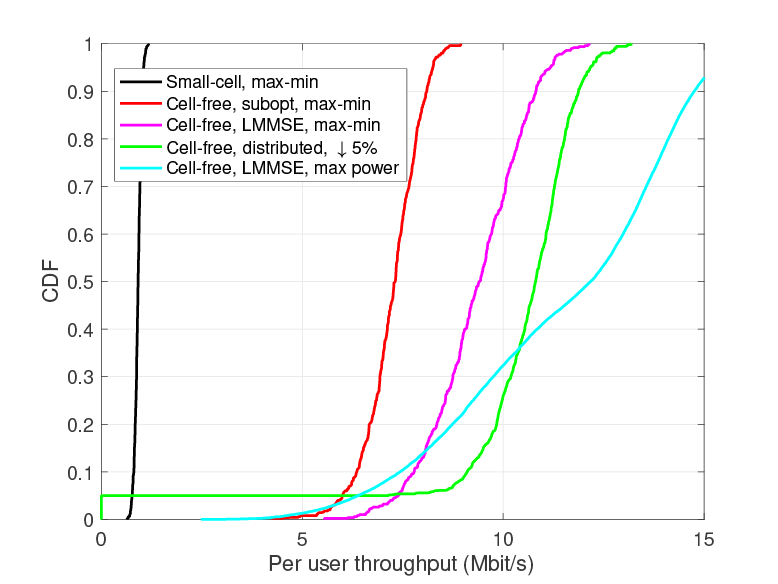
Figure 1: CDF of uplink user throughputs with uncorrelated shadow fading. $M=128,K=40,\tau=60$, cell size $D=100$ m and $\rho_{u}=\rho_{p}=20$ mW.

A similar effect is observed in Fig. 2 with correlated shadow fading and $D=500$ m. Based on the results in [17], cell-free systems exhibit slower channel hardening, capacity lower bounds that rely on channel hardening (such as our “use-then-forget” achievable rate bound) can be quite loose. Therefore, our performance estimates for the 50% likely throughput are conservative.

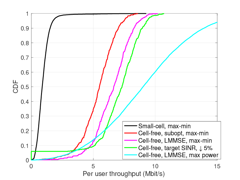
Figure 2: CDF of uplink user throughputs with correlated shadow fading. $M=128,K=40,\tau=60$, cell size $D=500$ m and $\rho_{u}=\rho_{p}=20$ mW.

In Fig. 3 and Fig. 4 we present results on the energy efficiency obtained with small-cell and cell-free systems with different power control algorithms. We observe that in terms of the energy efficiency power control algorithms and LMMSE channel estimation give even larger gains, than in terms of uplink data rates. In particular, systems with LMSSE channel estimation and max-min power control and and distributed power control gain 150% and 180% respectively over maximal power transmission. They also gain 74% and 95% respectively compared with the systems with suboptimal channel estimation and max-min power control. Similar results hold for correlated users, Fig. 4.

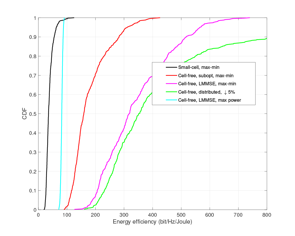
Figure 3: CDF of the energy efficiency of uncorrelated users. $M=128,K=40,\tau=60$, cell size $D=500$ m and $\rho_{u}=\rho_{p}=20$ mW.

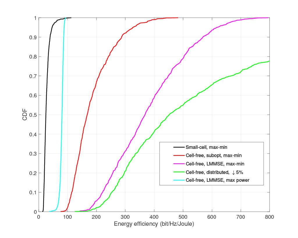
Figure 4: CDF of the energy efficiency of correlated users. $M=128,K=40,\tau=60$, cell size $D=500$ m and $\rho_{u}=\rho_{p}=20$ mW.

Uplink Experiment 2: Here, we assume a mobile phone communication scenario, rather than IoT scenario. We assume $D=1$ km and the transmit power $\rho_{u}=\rho_{p}=200$ mW, and uncorrelated shadow fading. Results are presented in Fig. 5. It can be seen that the cell-free systems outperform the small-cell system in both the median and the $95\%$-outage rate. In particular, in terms of the $95\%$-outage rate, the cell-free system with suboptimal channel estimation gives a $5$-fold improvement. The cell-free system with LMMSE channel estimation and max-min power control gives a 50% improvement in terms of $95\%$-outage rate. The system with the distributed power control and $5\%$ users dropping, that is 2 users in our settings, the median throughput can be further improved by about $10\%$. Note also that the $95\%$-outage rate with optimal channel estimation is about $50\%$ greater than in the case of no power control (max power).

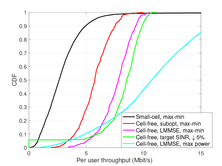
Figure 5: CDF of uplink user throughputs with uncorrelated shadow fading. $K=40,\tau=20$, cell size $D=1$ km and $\rho_{u}=\rho_{p}=200$ mW.

Fig. 6 presents results for the scenario with correlated shadow fading. One can see that correlated shadowing results in significant reduction of the throughputs. Still, the $95\%$-outage rate likely throughput of the cell-free system with LMMSE channel estimation and distributed power control is around 10 times higher than that of small-cell. It is important to note that the $95\%$-outage rate of cell-free system with the optimal channel estimation is twice that of the system with suboptimal channel estimation. These energy efficiency gains can be crucially important for IoT systems.

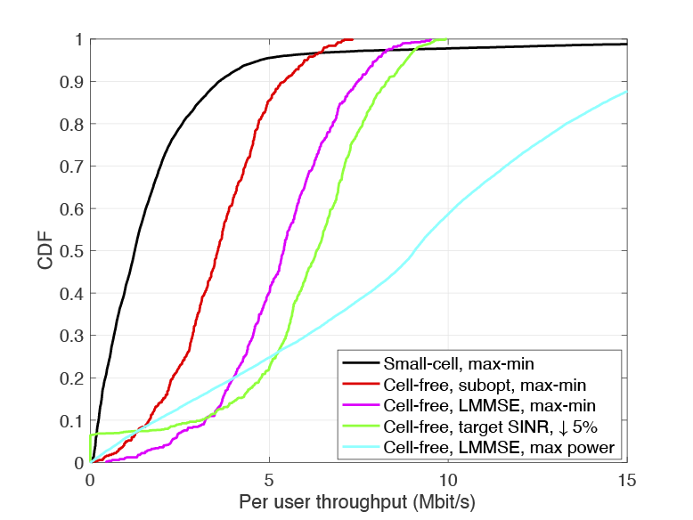
Figure 6: CDF of uplink user throughputs with correlated shadow fading. $K=40,\tau=20$, cell size $D=1$ km and $\rho_{u}=\rho_{p}=200$ mW.

Downlink Experiment 1: In this scenario, we consider the downlink throughputs with $M=128,\,K=20,\,\tau=40$. The cell size $D=100$ m, the shadow fading is uncorrelated and $\rho_{u}=\rho_{d}=20$ mW. Fig. 7 shows the per-user downlink throughput. The cell-free throughputs are about three times the throughput of the small-cell system. With LMMSE channel estimation, the 95% outage-rate of the cell-free system is about 25% higher than with suboptimal channel estimation.

A similar result is seen for correlated shadow fading in Fig. 8. Here, the 95% outage-rate with optimal channel estimation is about 40% higher than with suboptimal channel estimation.

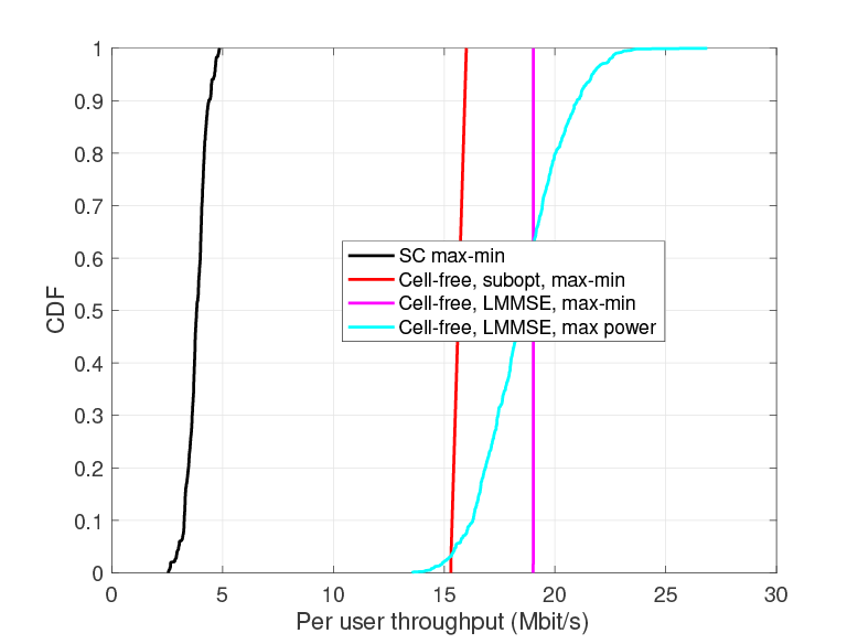
Figure 7: CDF of downlink user throughputs with uncorrelated shadow fading. $K=20,\tau=40$, cell size $D=100$ m and $\rho_{u}=\rho_{p}=20$ mW.

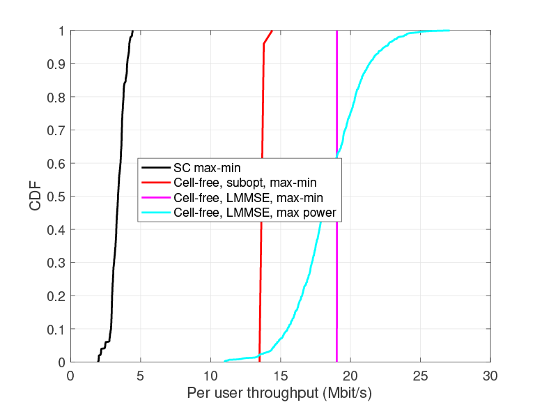
Figure 8: CDF of downlink user throughputs with correlated shadow fading. $K=20,\tau=40$, cell size $D=100$ m and $\rho_{u}=\rho_{p}=20$ mW.

Downlink Experiment 2: In this case, we assume a mobile phone communication scenario with $D=1$km, $\rho_{u}=\rho_{d}=200$ mW and uncorrelated shadow fading. The results are shown in Fig. 9. Both in the median and the 95% outage-rate, the cell-free systems outperform the small-cell system. The throughput with LMMSE channel estimation is about 28% higher than the cell-free system with suboptimal channel estimation.

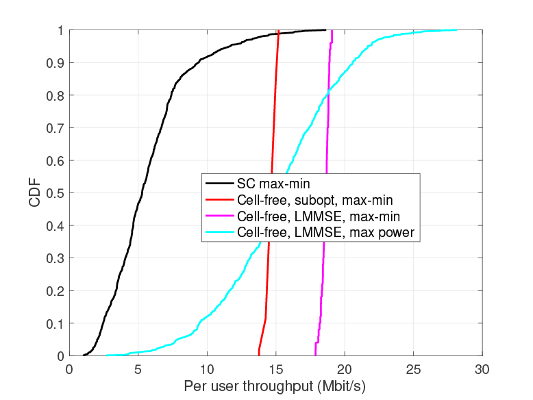
Figure 9: CDF of downlink user throughputs with correlated shadow fading. $K=20,\tau=10$, cell size $D=1$ km and $\rho_{u}=\rho_{p}=200$ mW.

IX Conclusion

We considered cell-free massive MIMO for IoT with optimal (LMMSE) channel estimation and random uplink pilots. The goal for studying such system was to considerably improve the spectral efficiency of both uplink and downlink transmissions compared with cell-free massive MIMO systems with sub-optimal channel estimation, and small-cell systems. The second goal was developing transmit power control algorithm that allow infrequent power adaptation, and provide additional improvement of the system performance (spectral efficiency). High energy efficiency is especially important for IoT because the things are operating under low power conditions. Centralized max-min SINR and distributed target SINR power control algorithms are utilized. Simulation results with max-min SINR power optimization show more than ten-fold improvement over conventional IoT systems based on small-cell architecture. A 40% improvement over cell-free systems with suboptimal channel estimation is achieved in terms of uplink data rates and 95% in terms of energy efficiency. Similarly, in the downlink, a three-fold improvement over small-cell systems was observed along with a maximum of 40% improvement in the downlink throughput over cell-free systems using suboptimal channel estimation.

Appendix A

For $T_{1}$ we have

$$T_{1}=\sqrt{\rho_{u}\eta_{k}}\sum_{m=1}^{M}\mathbb{E}[(\hat{g}_{mk}+\tilde{g}_{mk})\hat{g}^{*}_{mk}]=\sqrt{\rho_{u}\eta_{k}}\sum_{m=1}^{M}\mathbb{E}[|\hat{g}_{mk}|^{2}]=\sqrt{\rho_{u}\eta_{k}}\sum_{m=1}^{M}\gamma_{mk}.$$ (26)

It is easy find the variance of $T_{4}$ is

$$\mathbb{E}[|{\rm T_{4}}|^{2}]=\sum_{m=1}^{M}\gamma_{mk}.$$

Finding the variances of $T_{2}$ and $T_{3}$ require longer calculations, which are presented below.

$$\mathbb{E}[|T_{2}|^{2}]= \rho_{u}\eta_{k}\sum_{m=1}^{M}\sum_{n=1}^{M}\mathbb{E}[(\hat{g}^{*}_{mk}g_{mk}-\mathbb{E}[\hat{g}^{*}_{mk}g_{mk}])(\hat{g}_{nk}g^{*}_{nk}-\mathbb{E}[\hat{g}_{nk}g^{*}_{nk}])]$$ (27)

$$= \rho_{u}\eta_{k}\sum_{m=1}^{M}\sum_{n=1}^{M}[\mathbb{E}[\hat{g}^{*}_{mk}g_{mk}\hat{g}_{nk}g^{*}_{nk}]-\mathbb{E}[\hat{g}^{*}_{mk}g_{mk}]\gamma_{nk}-\mathbb{E}[\hat{g}_{nk}g^{*}_{nk}]\gamma_{mk}]+\rho_{u}\eta_{k}\sum_{m=1}^{M}\sum_{n=1}^{M}\gamma_{mk}\gamma_{nk}$$

$$= \rho_{u}\eta_{k}\sum_{m=1}^{M}\sum_{n=1}^{M}\mathbb{E}[\hat{g}^{*}_{mk}(\hat{g}_{mk}+\tilde{g}_{mk})\hat{g}_{nk}(\hat{g}^{*}_{nk}+\tilde{g}^{*}_{nk})]-\rho_{u}\eta_{k}\sum_{m=1}^{M}\sum_{n=1}^{M}\gamma_{mk}\gamma_{nk}$$

$$= \rho_{u}\eta_{k}\sum_{m=1}^{M}\sum_{n=1}^{M}\{\mathbb{E}[|\hat{g}_{mk}|^{2}|\hat{g}_{nk}|^{2}]+\mathbb{E}[|\hat{g}_{mk}|^{2}\hat{g}_{nk}\tilde{g}^{*}_{nk}]+\mathbb{E}[|\hat{g}_{nk}|^{2}\hat{g}^{*}_{mk}\tilde{g}_{mk}]+.$$

$$\hskip 142.26378pt.\underbrace{\mathbb{E}[\hat{g}^{*}_{mk}\tilde{g}_{mk}\hat{g}_{nk}\tilde{g}^{*}_{nk}]}_{=0\,{\rm if}\,m\neq n}\}-\rho_{u}\eta_{k}\sum_{m=1}^{M}\sum_{n=1}^{M}\gamma_{mk}\gamma_{nk}$$

$$\hskip 56.9055pt.\sum_{n=1}^{M}\{\mathbb{E}[|\hat{g}_{mk}|^{2}\hat{g}_{nk}\tilde{g}^{*}_{nk}]+\mathbb{E}[|\hat{g}_{nk}|^{2}\tilde{g}_{mk}\hat{g}^{*}_{mk}]\}]-\rho_{u}\eta_{k}\sum_{m=1}^{M}\sum_{n=1}^{M}\gamma_{mk}\gamma_{nk}$$

$$= \rho_{u}\eta_{k}\sum_{m=1}^{M}[2\gamma^{2}_{mk}+\gamma_{mk}(\beta_{mk}-\gamma_{mk})+\underbrace{\mathbb{E}[|\hat{g}_{mk}|^{2}\hat{g}_{mk}\tilde{g}^{*}_{mk}]+\mathbb{E}[|\hat{g}_{mk}|^{2}\hat{g}^{*}_{mk}\tilde{g}_{mk}]}_{=0}+.$$

$$.\hskip 28.45274pt\sum_{n\neq m}\{\gamma_{mk}\gamma_{nk}+\underbrace{\mathbb{E}[|\hat{g}_{mk}|^{2}\hat{g}_{nk}\tilde{g}^{*}_{nk}]+\mathbb{E}[|\hat{g}_{nk}|^{2}\hat{g}^{*}_{mk}\tilde{g}_{mk}]}_{=0}\}-\sum_{n=1}^{M}\gamma_{mk}\gamma_{nk}]$$

$$= \rho_{u}\eta_{k}\sum_{m=1}^{M}[\beta_{mk}\gamma_{mk}+\sum_{n=1}^{M}\gamma_{mk}\gamma_{nk}]-\rho_{u}\eta_{k}\sum_{m=1}^{M}\sum_{n=1}^{M}\gamma_{mk}\gamma_{nk}=\rho_{u}\eta_{k}\sum_{m=1}^{M}\gamma_{mk}\beta_{mk}.$$

Further,

$$\mathbb{E}[|T_{3}|^{2}]=\sum_{i\neq k}\mathbb{E}[|v_{i}|^{2}].$$

We will consider individual terms of this sum:

$$\mathbb{E}[|v_{i}|^{2}]= \rho_{u}\eta_{i}\mathbb{E}[|\sum_{m=1}^{M}g_{mi}\hat{g}^{*}_{mk}|^{2}]$$

$$= \rho_{u}\eta_{i}\mathbb{E}[|\sum_{m=1}^{M}g_{mi}({\bf a}^{H}_{m,k}[\sqrt{\tau\rho_{p}}\boldsymbol{\Psi}{\bf g}_{m}+{\bf w}_{m}])^{*}|^{2}]$$

$$= \rho_{u}\eta_{i}\mathbb{E}[|\sum_{m=1}^{M}g_{mi}\sum_{j=1}^{K}\sqrt{\tau\rho_{p}}g^{*}_{mj}\boldsymbol{\psi}^{H}_{j}{\bf a}_{m,k}+\sum_{m=1}^{M}g_{mi}{\bf w}^{H}_{m}{\bf a}_{m,k}|^{2}]$$

$$= \rho_{u}\eta_{i}\tau\rho_{p}\mathbb{E}[|\sum_{m=1}^{M}g_{mi}\sum_{j=1}^{K}g^{*}_{mj}\boldsymbol{\psi}^{H}_{j}{\bf a}_{m,k}|^{2}]+\rho_{u}\eta_{i}\mathbb{E}[|\sum_{m=1}^{M}g_{mi}{\bf w}^{H}_{m}{\bf a}_{m,k}|^{2}]$$

$$= \rho_{u}\eta_{i}\sum_{m=1}^{M}\beta_{mi}\lVert{\bf a}_{m,k}\rVert^{2}_{2}+\rho_{u}\eta_{i}\tau\rho_{p}\underbrace{\sum_{m=1}^{M}\sum_{n=1}^{M}\sum_{j=1}^{K}\sum_{l=1}^{K}\mathbb{E}[g_{mi}g^{*}_{mj}g^{*}_{ni}g_{nl}\boldsymbol{\psi}^{H}_{j}{\bf a}_{m,k}{\bf a}^{H}_{n,k}\boldsymbol{\psi}_{l}]}_{\mathcal{T}_{i}}.$$ (28)

For finding $\mathcal{T}_{i}$ we first note that

$$\mathbb{E}[g_{mi}g^{*}_{mj}g^{*}_{ni}g_{nl}]= \begin{cases}{\rm if}\,m=n\begin{cases}\mathbb{E}[|g_{mi}|^{4}]=2\beta^{2}_{mi},\quad{\rm if}\,j=l=i,\\ \mathbb{E}[|g_{mi}|^{2}|g_{mj}|^{2}]=\beta_{mi}\beta_{mj},\quad{\rm if}\,j=l\neq i,\\ 0,\quad{\rm otherwise.}\\ \end{cases}\\ {\rm if}\,m\neq n\begin{cases}\mathbb{E}[|g_{mi}|^{2}|g_{ni}|^{2}]=\beta_{mi}\beta_{ni},\quad{\rm if}\,j=l=i,\\ 0,\quad{\rm otherwise.}\\ \end{cases}\end{cases}$$ (29)

Thus,

$$\mathcal{T}_{i}=\sum_{m=1}^{M}(2\beta^{2}_{mi}|\boldsymbol{\psi}^{H}_{i}{\bf a}_{m,k}|^{2}+\sum_{j\neq i}^{K}\beta_{mi}\beta_{mj}|\boldsymbol{\psi}^{H}_{j}{\bf a}_{m,k}|^{2}+\sum_{n\neq m}\beta_{mi}\beta_{ni}\boldsymbol{\psi}^{H}_{i}{\bf a}_{m,k}{\bf a}^{H}_{n,k}\boldsymbol{\psi}_{i}).$$ (30)

Using these results, we obtain

$$\mathbb{E}[|T_{3}|^{2}]= \rho_{u}\eta_{i}\sum_{m=1}^{M}\beta_{mi}{\bf a}^{H}_{m,k}{\bf a}_{m,k}+\rho_{u}\eta_{i}\tau\rho_{p}\sum_{m=1}^{M}(\sum_{n=1}^{M}\beta_{mi}\beta_{ni}\boldsymbol{\psi}^{H}_{i}{\bf a}_{m,k}{\bf a}^{H}_{n,k}\boldsymbol{\psi}_{i}+\sum_{j=1}^{K}\beta_{mi}\beta_{mj}|\boldsymbol{\psi}^{H}_{j}{\bf a}_{m,k}|^{2}).$$ (31)

Appendix B

To prove the theorem, we have to show that the functions $I_{k}(\boldsymbol{\eta})=\frac{\eta_{k}}{{\rm SINR}_{k}^{u}}$ and $1/I_{k}(\boldsymbol{\eta})$ are two-sided scalable [12, 13].

A function $I(\boldsymbol{\eta})$ is two-sided scalable if for any $\alpha>1$, and vectors $\boldsymbol{\eta}_{1}$ and $\boldsymbol{\eta}_{2}$ we have $\frac{1}{\alpha}I(\boldsymbol{\eta}_{1})<I(\boldsymbol{\eta}_{2})<\alpha I(\boldsymbol{\eta}_{1})$, if $\frac{1}{\alpha}\boldsymbol{\eta}_{1}<\boldsymbol{\eta}_{2}<\alpha\boldsymbol{\eta}_{1}$.

We first show that $I_{k}(\boldsymbol{\eta})$ is a standard interference function, i.e., it satisfies the following conditions:

1. $I_{k}(\boldsymbol{\eta})\geq 0,\forall\boldsymbol{\eta}\geq 0$,

2. $I_{k}(\boldsymbol{\eta}_{1})\geq I_{k}(\boldsymbol{\eta}_{2})$, if $\boldsymbol{\eta}_{1}\geq\boldsymbol{\eta}_{2}$,

3. For $\alpha>1,I_{k}(\alpha\boldsymbol{\eta})<\alpha I_{k}(\boldsymbol{\eta})$.

It can be seen that $I_{k}(\boldsymbol{\eta})\geq 0$ since both $\boldsymbol{\eta}$ and ${\rm SINR}_{k}^{u}$ are positive. To show that condition (ii) holds, we write $I_{k}(\boldsymbol{\eta})$ in the form

$$I_{k}(\boldsymbol{\eta})=$$ (32)

$$\frac{\sum\limits_{m=1}^{M}\gamma_{mk}(\frac{1}{\rho_{u}}+\eta_{k}\beta_{mk})+\sum\limits_{i\neq k}\eta_{i}[\sum\limits_{m=1}^{M}\beta_{mi}\lVert{\bf a}_{m,k}\rVert^{2}_{2}+\tau\rho_{p}(|\sum\limits_{m=1}^{M}\beta_{mi}\boldsymbol{\psi}^{H}_{i}{\bf a}_{m,k}|^{2}+\sum\limits_{m=1}^{M}\sum\limits_{j=1}^{K}\beta_{mi}\beta_{mj}|\boldsymbol{\psi}^{H}_{j}{\bf a}_{m,k}|^{2})]}{(\sum\limits_{m=1}^{M}\gamma_{mk})^{2}}.$$

Now, let $\eta^{(1)}_{k}$ be $k$-th element of $\boldsymbol{\eta}_{1}$. Then we have

$$I_{k}(\boldsymbol{\eta}_{1})$$ (33)

$$=\frac{\sum\limits_{m=1}^{M}\gamma_{mk}(\frac{1}{\rho_{u}}+\eta^{(1)}_{k}\beta_{mk})+\sum\limits_{i\neq k}\eta_{i}^{(1)}[\sum\limits_{m=1}^{M}\beta_{mi}\lVert{\bf a}_{m,k}\rVert^{2}_{2}+\tau\rho_{p}(|\sum\limits_{m=1}^{M}\beta_{mi}\boldsymbol{\psi}^{H}_{i}{\bf a}_{m,k}|^{2}+\sum\limits_{m=1}^{M}\sum\limits_{j=1}^{K}\beta_{mi}\beta_{mj}|\boldsymbol{\psi}^{H}_{j}{\bf a}_{m,k}|^{2})]}{(\sum\limits_{m=1}^{M}\gamma_{mk})^{2}}$$

$$\geq\frac{\sum\limits_{m=1}^{M}\gamma_{mk}(\frac{1}{\rho_{u}}+\eta^{(2)}_{k}\beta_{mk})+\sum\limits_{i\neq k}\eta_{i}^{(2)}[\sum\limits_{m=1}^{M}\beta_{mi}\lVert{\bf a}_{m,k}\rVert^{2}_{2}+\tau\rho_{p}(|\sum\limits_{m=1}^{M}\beta_{mi}\boldsymbol{\psi}^{H}_{i}{\bf a}_{m,k}|^{2}+\sum\limits_{m=1}^{M}\sum\limits_{j=1}^{K}\beta_{mi}\beta_{mj}|\boldsymbol{\psi}^{H}_{j}{\bf a}_{m,k}|^{2})]}{(\sum\limits_{m=1}^{M}\gamma_{mk})^{2}}$$

$$=I_{k}(\boldsymbol{\eta}_{2}),$$

where the inequality holds due to linearity of the numerator term.

To show that condition (iii) holds, we notice that for $\alpha>1$ we have

$$I_{k}(\alpha\boldsymbol{\eta})$$ (34)

$$=\frac{\sum\limits_{m=1}^{M}\gamma_{mk}(\frac{1}{\rho_{u}}+\alpha\eta_{k}\beta_{mk})+\sum\limits_{i\neq k}\alpha\eta_{i}\left[\sum\limits_{m=1}^{M}\beta_{mi}\lVert{\bf a}_{m,k}\rVert^{2}_{2}+\tau\rho_{p}\left(|\sum\limits_{m=1}^{M}\beta_{mi}\boldsymbol{\psi}^{H}_{i}{\bf a}_{m,k}|^{2}+\sum\limits_{m=1}^{M}\sum\limits_{j=1}^{K}\beta_{mi}\beta_{mj}|\boldsymbol{\psi}^{H}_{j}{\bf a}_{m,k}|^{2}\right)\right]}{\left(\sum\limits_{m=1}^{M}\gamma_{mk}\right)^{2}}$$

$$<\frac{\alpha\sum\limits_{m=1}^{M}\gamma_{mk}(\frac{1}{\rho_{u}}+\eta_{k}\beta_{mk})+\sum\limits_{i\neq k}\alpha\eta_{i}\left[\sum\limits_{m=1}^{M}\beta_{mi}\lVert{\bf a}_{m,k}\rVert^{2}_{2}+\tau\rho_{p}\left(|\sum\limits_{m=1}^{M}\beta_{mi}\boldsymbol{\psi}^{H}_{i}{\bf a}_{m,k}|^{2}+\sum\limits_{m=1}^{M}\sum\limits_{j=1}^{K}\beta_{mi}\beta_{mj}|\boldsymbol{\psi}^{H}_{j}{\bf a}_{m,k}|^{2}\right)\right]}{\left(\sum\limits_{m=1}^{M}\gamma_{mk}\right)^{2}}$$

$$=\alpha I_{k}(\boldsymbol{\eta}).$$

Now, let $\boldsymbol{\eta}=\frac{\boldsymbol{\eta}}{\alpha}$. Then, from (iii), we get $\frac{1}{\alpha}I_{k}(\boldsymbol{\eta})<I_{k}(\frac{\boldsymbol{\eta}}{\alpha})$. If $\frac{1}{\alpha}\boldsymbol{\eta}_{1}<\boldsymbol{\eta}_{2}<\alpha\boldsymbol{\eta}_{1}$, then

$$\frac{1}{\alpha}I_{k}(\boldsymbol{\eta}_{1})<I_{k}(\frac{\boldsymbol{\eta}_{1}}{\alpha})\stackrel{{\scriptstyle\text{(a)}}}{{<}}I_{k}(\boldsymbol{\eta}_{2})\stackrel{{\scriptstyle\text{(b)}}}{{<}}I_{k}(\alpha\boldsymbol{\eta}_{1})\stackrel{{\scriptstyle\text{(c)}}}{{<}}\alpha I_{k}(\boldsymbol{\eta}_{1}),$$

where (a) and (b) follow from condition (ii) and (c) follows from condition (iii). Thus,

$$\frac{1}{\alpha}I_{k}(\boldsymbol{\eta}_{1})<I_{k}(\boldsymbol{\eta}_{2})<\alpha I_{k}(\boldsymbol{\eta}_{1}),$$

and $I_{k}(\boldsymbol{\alpha})$ is a two-sided scalable function. From this, we can also show that

$$\frac{1}{\alpha I_{k}(\boldsymbol{\eta}_{1})}<\frac{1}{I_{k}(\boldsymbol{\eta}_{2})}<\alpha\frac{1}{I_{k}(\boldsymbol{\eta}_{1})}.$$

Thus, $\frac{1}{I_{k}(\boldsymbol{\eta})}$ is also two-sided scalable.

Appendix C

It is easy to see that

$$\mathbb{E}[|T_{1}|^{2}]=\rho_{d}\left(\sum_{m=1}^{M}\eta_{mk}^{1/2}\gamma_{mk}\right)^{2}\mbox{ and }\mathbb{E}[|{\rm T_{4}}|^{2}]=1.$$

.

The variances of $T_{2}$ and $T_{3}$ are calculated similarly as in Appendix A.

References

- [1] L. Liu and W. Yu, “Massive connectivity with massive MIMO- Part I: Device activity detection and channel estimation,” IEEE Trans. Signal Process., vol. 66, no. 11, pp. 2933–2946.
- [2] L. Liu and W. Yu, “Massive connectivity with massive MIMO- Part II: Achievable rate characterization,” IEEE Trans. Signal Process., vol. 66, no. 11, pp. 2947–2959, 2018.
- [3] B. M. Lee and H. Yang, “Massive MIMO for industrial internet of things in cyber-physical systems,” IEEE Trans. Ind. Informat., vol. 14, no. 6, pp. 2641–2652, 2018.
- [4] B. M. Lee and H. Yang, “Massive MIMO with massive connectivity for Industrial Internet of Things,” IEEE Trans. Ind. Electron., vol. 67, no. 6, pp. 5187–5196, 2020.
- [5] H. Q. Ngo, A. Ashikhmin, H. Yang, E. G. Larsson, and T. L. Marzetta, “Cell-free massive MIMO versus small cells,” IEEE Trans. Wireless Commun., vol. 16, no. 3, pp. 1834–1850, March 2017.
- [6] E. Nayebi, A. Ashikhmin, T. L. Marzetta, H. Yang, and B. D. Rao, “Precoding and power optimization in cell-free massive MIMO systems,” IEEE Trans. Wireless Commun., vol. 16, no. 7, pp. 4445–4459, 2017.
- [7] Z. Liu and L. Dai, “A comparative study of downlink MIMO cellular networks with co-located and distributed base-station antennas,” IEEE Trans. Wireless Commun., vol. 13, no. 11, pp. 6259–6274, Nov 2014.
- [8] W. Liu, S. Han, and C. Yang, “Energy efficiency comparison of massive MIMO and small cell network,” in Proc. Global Conf. Signal Inf. Processing. IEEE, 2014, pp. 617–621.
- [9] B. Hassibi and B. M. Hochwald, “How much training is needed in multiple-antenna wireless links?,” IEEE Trans. Inf. Theory, vol. 49, no. 4, pp. 951–963, 2003.
- [10] H. Q. Ngo, E. G. Larsson, and T. L. Marzetta, “Energy and spectral efficiency of very large multiuser MIMO systems,” IEEE Trans. Commun., vol. 61, no. 4, pp. 1436–1449, April 2013.
- [11] H. Yang and T. L. Marzetta, “Capacity performance of multicell large-scale antenna systems,” in Proc. Allerton Conf. on Commun., Control and Comput., Oct 2013, pp. 668–675.
- [12] M. Rasti and A. R. Sharafat, “Distributed uplink power control with soft removal for wireless networks,” IEEE Trans. Commun., vol. 59, no. 3, pp. 833–843, 2011.
- [13] A. Adhikary, A. Ashikhmin, and T. L. Marzetta, “Uplink interference reduction in large-scale antenna systems,” IEEE Trans. Commun., vol. 65, no. 5, pp. 2194–2206, 2017.
- [14] H. Yang and T. L. Marzetta, “Energy efficiency of Massive MIMO: Cell-free vs. Cellular,” in IEEE 87th Veh. Technol. Conf. (VTC Spring), 2018, pp. 1–5.
- [15] M. Grant and S. Boyd, “CVX: Matlab software for disciplined convex programming, version 2.1,” http://cvxr.com/cvx, Mar. 2014.
- [16] A. Tang, J. Sun, and K. Gong, “Mobile propagation loss with a low base station antenna for NLOS street microcells in urban area,” in Vehicular Technology Conference. IEEE, 2001, vol. 1, pp. 333–336.
- [17] Z. Chen and E. Björnson, “Channel hardening and favorable propagation in cell-free massive MIMO with stochastic geometry,” IEEE Trans. Commun., vol. 66, no. 11, pp. 5205–5219, 2018.