Abstract

Stochastic Gradient Descent (SGD) is being used routinely for optimizing non-convex functions. Yet, the standard convergence theory for SGD in the smooth non-convex setting gives a slow sublinear convergence to a stationary point. In this work, we provide several convergence theorems for SGD showing convergence to a global minimum for non-convex problems satisfying some extra structural assumptions. In particular, we focus on two large classes of structured non-convex functions: (i) Quasar (Strongly) Convex functions (a generalization of convex functions) and (ii) functions satisfying the Polyak-Lojasiewicz condition (a generalization of strongly-convex functions). Our analysis relies on an Expected Residual condition which we show is a strictly weaker assumption than previously used growth conditions, expected smoothness or bounded variance assumptions. We provide theoretical guarantees for the convergence of SGD for different step-size selections including constant, decreasing and the recently proposed stochastic Polyak step-size. In addition, all of our analysis holds for the arbitrary sampling paradigm, and as such, we give insights into the complexity of minibatching and determine an optimal minibatch size. Finally, we show that for models that interpolate the training data, we can dispense of our Expected Residual condition and give state-of-the-art results in this setting.

1 INTRODUCTION

We consider the unconstrained finite-sum optimization problem

$$\min_{x\in\mathbb{R}^{d}}\left[f(x)=\frac{1}{n}\sum_{i=1}^{n}f_{i}(x)\right].$$ (1)

We use ${\cal X}^{*}\subset\mathbb{R}^{d}$ to denote the set of minimizers $x^{*}$ of (1) and assume that ${\cal X}^{*}$ is not empty and that $f(x)$ is lower bounded. This problem is prevalent in machine learning tasks where $x$ corresponds to the model parameters, $f_{i}(x)$ represents the loss on the training point $i$ and the aim is to minimize the average loss $f(x)$ across training points.

When $n$ is large, stochastic gradient descent (SGD) and its variants are the preferred methods for solving (1) mainly because of their cheap per iteration cost. The standard convergence theory for SGD (Robbins and Monro,, 1951; Nemirovski and Yudin,, 1978, 1983; Shalev-Shwartz et al.,, 2007; Nemirovski et al.,, 2009; Arjevani et al.,, 2019; Hardt et al.,, 2016) in the smooth nonconvex setting shows slow sub-linear convergence to a stationary point. Yet in contrast, when applying SGD to many practical nonconvex problems of the form (1) such as matrix completion (Sa et al.,, 2015), deep learning (Ma et al.,, 2018), and phase retrieval (Tan and Vershynin,, 2019) the iterates converge globally, and sometimes, even linearly. This is because these problems often have additional structure and properties, such as all local minimas are global minimas (Sa et al.,, 2015; Kawaguchi,, 2016), the model interpolates the data (Ma et al.,, 2018) or the function under study is unimodal on all lines through a minimizer (Hinder et al.,, 2020). By exploiting these structures and properties one can prove significantly tighter convergence bounds.

Here we present a general analysis of SGD for two large classes of structured nonconvex functions: (i) the Quasar (Strongly) Convex functions and (ii) functions satisfying the Polyak-Lojasiewicz (PL) condition. In all of our results we provide convergence guarantees for SGD to the global minimum. We also develop several corollaries for functions that interpolate the data.

1.1 Background and Main Contributions

Classes of structured nonconvex functions. The last few years has seen an increased interest in exploiting additional structure prevalent in large classes of nonconvex functions. Such conditions include error bound properties (Fabian et al.,, 2010), essential strong convexity (Liu et al.,, 2014), quasi strong convexity (Necoara et al.,, 2018; Gower et al.,, 2019), the restricted secant inequality (Zhang and Yin,, 2013), and the quadratic growth (QG) condition (Anitescu,, 2000; Loizou,, 2019). We focus on two of the weakest conditions: the quasar (strongly) convex functions (Hinder et al.,, 2020; Hardt et al.,, 2018; Guminov and Gasnikov,, 2017) and functions satisfying the PL condition (Polyak,, 1987; Lojasiewicz,, 1963; Karimi et al.,, 2016). The class of quasar-convex functions include all convex functions as a special case, but it also includes several nonconvex functions. Recently there is also some evidences suggesting that the loss function of neural networks have a quasar-convexity structure (Zhou et al.,, 2019; Kleinberg et al.,, 2018).

Contributions. We show that SGD converges at a ${\cal O}(1/\sqrt{k})$ rate on the quasar-convex functions and prove linear convergence to a neighborhood for PL functions without any bounded variance assumption or growth assumptions on the stochastic gradients. Instead, we rely on the recently introduced expected residual (ER) condition (Gower et al.,, 2020).

Assumptions on the gradient. The standard convergence analysis of SGD in the nonconvex setting relies on the bounded gradients assumption $\mathbb{E}_{i}\|\nabla f_{i}(x^{k})\|^{2}<c$ (Recht et al.,, 2011; Hazan and Kale,, 2014; Rakhlin et al.,, 2012) or a growth condition $\mathbb{E}_{i}\|\nabla f_{i}(x^{k})\|^{2}\leq c_{1}+c_{2}\mathbb{E}\|\nabla f(x^{k})\|^{2}$ (Bertsekas and Tsitsiklis,, 1996; Bottou et al.,, 2018; Schmidt et al.,, 2017). There is now a line of recent works (Nguyen et al.,, 2018; Vaswani et al., 2019a, ; Gower et al.,, 2019; Khaled and Richtarik,, 2020; Lei et al.,, 2019; Koloskova et al.,, 2020; Loizou et al.,, 2020) which aims at relaxing these assumptions.

Contributions. We use the recently introduced Expected Residual (ER) condition (Gower et al.,, 2020). We give the first convergence proofs for SGD under the 3.1 condition and we show that 3.1 is a strictly weaker assumption than the Strong Growth Condition (SGC) (Schmidt and Roux,, 2013), Weak Growth (WGC) (Vaswani et al., 2019a, ) or the Expected Smoothness (ES) (Gower et al.,, 2019) assumptions. Furthermore, we show that the 3.1 condition holds for a large class of nonconvex functions including 1) smooth and interpolated functions 2) smooth and $x^{*}$– convex functions. Not only does the ER assumption hold for a larger class of functions, our resulting convergence rates under ER either match or exceed the state-of-the-art for quasar-convex and PL functions.

PL condition. The PL condition (Polyak,, 1987; Lojasiewicz,, 1963) was introduced as a sufficient condition for the linear convergence of Gradient Descent for nonconvex functions. Assuming bounded gradients, it was shown in Karimi et al., (2016) that SGD with a decreasing step size converges sublinearly at a rate of ${\cal O}(1/\sqrt{k})$ for PL functions. In contrast, by using a step size which depends on the total number of iterations, the same convergence rate can be achieved without the need for the bounded gradient assumption (Khaled and Richtarik,, 2020). Assuming in addition the interpolation condition and SGC Vaswani et al., 2019a showed that SGD converges linearly for PL functions, but the specialization of this last result to gradient descent results in a suboptimal dependence on the condition number of the function.

Contributions. We provide a complete minibatch analysis of SGD for PL functions which recovers the best known dependence on the condition number for Gradient Descent (Karimi et al.,, 2016) while also matching the current state-of-the-art rate derived in Vaswani et al., 2019a ; Lei et al., (2019) for SGD for interpolated functions. All of which relies on the weaker 3.1 condition. Moreover, we propose a switching step size scheme similar to Gower et al., (2019) which does not require knowledge of the last iterate of the algorithm. Using this step size, we prove that SGD converges sublinearly at a rate of ${\cal O}(1/k)$ for PL functions without any additional bounded gradient of bounded variance assumption or growth assumption.

Step-size selection for SGD. The most important parameter that one should select to guarantee the convergence of SGD is the step-size or learning rate. There are several choices that one can use including constant step-size (Moulines and Bach,, 2011; Needell et al.,, 2016; Gower et al.,, 2019; Needell and Ward,, 2017; Nguyen et al.,, 2018), decreasing step-size (Robbins and Monro,, 1951; Ghadimi and Lan,, 2013; Gower et al.,, 2019; Nemirovski et al.,, 2009; Karimi et al.,, 2016) and adaptive step-size Duchi et al., (2011); Liu et al., (2020); Kingma and Ba, (2015); Bengio, (2015); Vaswani et al., 2019b ; Ward et al., (2019).

Contributions. We provide convergence theorems for SGD under several step-size rules for minimizing quasar-convex functions and functions satisfying the PL condition, including constant and decreasing step-sizes and a recently introduced adaptive learning rate called the stochastic Polyak step-size (Loizou et al.,, 2020).

Over-parameterized models and Interpolation. Recently it was shown that SGD converges considerably faster when the underlying model is sufficiently over-parameterized as to interpolate the data. This includes problems such as deep matrix factorization (Rolinek and Martius,, 2018; Rahimi and Recht,, 2017), binary classification using kernels (Loizou et al.,, 2020), consistent linear systems (Gower and Richtárik,, 2015; Richtárik and Takác,, 2020; Loizou and Richtárik, 2020b, ; Loizou and Richtárik, 2020a, ) and multi-class classification using deep networks (Vaswani et al., 2019a, ; Loizou et al.,, 2020).

Contributions. As a corollary of our main theorems we show that for models that interpolate the training data, we can further relax our assumptions, dispense of the 3.1 condition altogether and instead, simply assume that each $f_{i}$ is smooth. Our results here match the state-of-the-art convergence results (Vaswani et al., 2019a, ) but again under strictly weaker assumptions.

1.2 SGD and Arbitrary Sampling

We assume we are given access to unbiased estimates $g(x)\in\mathbb{R}^{d}$ of the gradient such that ${\mathbb{E}\left[g(x)\right]}=\nabla f(x).$ For example, we can use a minibatch to form an estimate of the gradient such as $g(x)=\frac{1}{b}\sum_{i\in B}\nabla f_{i}(x),$ where $B\subset\{1,\ldots,n\}$ will be chosen uniformly at random and $|B|=b.$ To allow for any form of minibatching we use the arbitrary sampling notation

$$g(x)=\nabla f_{v}(x):=\frac{1}{n}\sum_{i=1}^{n}v_{i}\nabla f_{i}(x),$$ (2)

where $v\in\mathbb{R}^{n}_{+}$ is a random sampling vector such that ${\mathbb{E}\left[v_{i}\right]}=1,\,\mbox{for }i=1,\ldots,n$ and $f_{v}(x)~{}:=~{}\frac{1}{n}\sum_{i=1}^{n}v_{i}f_{i}(x)$. Note that it follows immediately from this definition of sampling vector that ${\mathbb{E}\left[g(x)\right]}=\frac{1}{n}\sum_{i=1}^{n}{\mathbb{E}\left[v_{i}\right]}\nabla f_{i}(x)=\nabla f(x).$ In this work we mostly focus on the $b$–minibatch sampling, however we highlight that our analysis holds for every form of minibatching.

Definition 1.1 (Minibatch sampling).

Let $b\in[n]$. We say that $v\in\mathbb{R}^{n}$ is a $b$–minibatch sampling if for every subset $S\in[n]$ with $|S|=b$ we have that

$$\mathbb{P}\left[v=\frac{n}{b}\sum_{i\in S}e_{i}\right]=\left.1\right/\binom{n}{b}:=\frac{b!(n-b)!}{n!}$$

By using a double counting argument you can show that if $v$ is a $b$–minibatch sampling, it is also a valid sampling vector (${\mathbb{E}\left[v_{i}\right]}=1$) (Gower et al.,, 2019). See Gower et al., (2019) for other choices of sampling vectors $v$.

With an unbiased estimate of the gradient $g(x)$, we can now use Stochastic gradient descent (SGD) to solve (1) by sampling $g(x^{k})$ i.i.d and iterating

$$\boxed{x^{k+1}=x^{k}-\gamma^{k}g(x^{k})}$$ (3)

We also make the following mild assumption on the gradient noise.

Assumption 1.2.

The gradient noise $\sigma^{2}$ is finite.

$$\sigma^{2}:=\sup_{x^{*}\in{\cal X}^{*}}{\mathbb{E}\left[\left\|g(x^{*})\right\|^{2}\right]}<\infty.$$

2 CLASSES OF STRUCTURED NONCONVEX FUNCTIONS

We work with two classes of nonconvex problems: the quasar-convex functions and the functions that satisfy the Polyak-Lojasiewicz (PL) condition.

Definition 2.1 (Quasar convex).

Let $\zeta\in(0,\,1]$ and $x^{*}\in{\cal X}^{*}$. We say that $f$ is $\zeta$- quasar-convex with respect to $x^{*}$ if for all $x\in\mathbb{R}^{n}$,

$$f(x^{*})\geq f(x)+\frac{1}{\zeta}\langle\nabla f(x),x^{*}-x\rangle.$$ (4)

For shorthand we write $f\in QC(\zeta)$ to mean (4). The class of quasar-convex functions are parameterized by a positive constant $\zeta\in(0,\,1]$. In the case that $\zeta=1$ then (4) is known as star convexity (Nesterov and Polyak,, 2006) (generalization of convexity). One can think of $\zeta$ as the value that controls the non-convexity of the function. As $\zeta$ becomes smaller the function becomes “more nonconvex” (Hinder et al.,, 2020).

One of weakest possible assumptions that guarantee a global convergence of gradient descent to the global minimum is the PL condition (Karimi et al.,, 2016). Indeed, all local minimas of a function satisfying the PL condition are also global minimas.

Definition 2.2 (Polyak-Lojasiewicz (PL) Condition).

There exists $\mu>0$ such that

$$\|\nabla f(x)\|^{2}\geq 2\mu\left[f(x)-f^{*}\right]$$ (5)

We write $f\in PL(\mu)$ if function $f$ satisfies (5).

In addition we will also consider in several corollaries the following interpolation condition.

Assumption 2.3.

We say that the interpolation condition holds if there exists $x^{*}\in{\cal X}^{*}$ such that

$$\min_{x\in\mathbb{R}^{n}}f_{i}(x)=f_{i}(x^{*})\quad\mbox{for}\quad i=1,\ldots,n.$$ (6)

This interpolation condition has drawn much attention recently because many overparametrized deep neural networks achieve a zero loss over all training data points (Ma et al.,, 2018) and thus satisfy (6).

3 EXPECTED RESIDUAL (ER)

In all of our analysis of SGD we rely on the Expected Residual (ER) assumption. In this section we formally define ER, provide new sufficient conditions for it to hold and relate it to the existing gradient assumptions.

ER measures how far the gradient estimate $g(x)$ is from the true gradient in the following sense.

Assumption 3.1 (Expected residual).

We say that the 3.1 condition holds or $g\in\text{ER}(\rho)$ if

$${\mathbb{E}\left[\left\|g(x)-g(x^{*})-(\nabla f(x)-\nabla f(x^{*}))\right\|^{2}\right]}$$

$$\leq 2\rho\left(f(x)-f(x^{*})\right),\quad\forall x\in\mathbb{R}^{d}.$$ (ER)

Note that 3.1 depends on both how $g(x)$ is sampled and the properties of the $f(x)$ function.

As a direct consequence of Assumption 3.1 we have the following bound on the variance of $g(x).$

Lemma 3.2.

If $g\in\text{ER}(\rho)$ then

$${\mathbb{E}\left[\|g(x)\|^{2}\right]}\leq 4\rho(f(x)-f^{*})+\|\nabla f(x)\|^{2}+2\sigma^{2}.$$ (7)

It is this bound on the variance (7) that we use in our proofs and allows us to avoid the stronger bounded gradient or bounded variance assumptions.

Connections to other Assumptions. Let us provide some more familiar sufficient conditions which guarantee that the 3.1 condition holds. In doing so, we will also provide simple and informative bounds on the expected residual constant $\rho$ when using minibatching.

We say that $f_{i}$ is $L_{i}$–smooth if $\forall x,z\in\mathbb{R}^{d}$ holds that:

$$f_{i}(z)-f_{i}(x) \;\leq\;\left<\nabla f_{i}(x),z-x\right>+\frac{L_{i}}{2}\left\|z-x\right\|^{2}.$$ (8)

Let $L_{\max}:=\max_{i=1,\ldots,n}L_{i}.$ For $x^{*}\in{\cal X}^{*}$, we say that $f_{i}$ is $x^{*}$–convex if

$$f_{i}(x^{*})-f_{i}(x) \;\leq\;\left<\nabla f_{i}(x^{*}),x^{*}-x\right>,\quad\forall x\in\mathbb{R}^{d}.$$ (9)

These two assumptions are sufficient for the $ER(\rho)$ condition to hold and give a useful bound on $\rho$, as we show in the following proposition.

Proposition 3.3.

Let $v$ be a sampling vector. If $f_{i}$ is $L_{i}$–smooth and there exists $x^{*}\in{\cal X}^{*}$ such that $f_{i}$ is $x^{*}$–convex then $g\in\text{ER}(\rho)$. If in addition $v$ is the $b$–minibatch sampling then

$$\rho(b)=L_{\max}\frac{n-b}{(n-1)b},\quad\sigma^{2}(b)=\frac{1}{b}\frac{n-b}{n-1}\sigma_{1}^{2},$$ (10)

where $\sigma_{1}^{2}:=\sup_{x^{*}\in{\cal X}^{*}}\frac{1}{n}\sum_{i=1}^{n}\left\|\nabla f_{i}(x^{*})\right\|^{2}.$

The bounds in Proposition 3.3 have been proven before but under the stronger assumption that each $f_{i}$ is convex. In this work by dropping the requirement that each $f_{i}$ is convex we are able to consider interesting classes of nonconvex functions.

Indeed, the following theorem establishes that only smoothness and the interpolation condition are sufficient for the 3.1 to hold. Furthermore, we place the 3.1 within a hierarchy of the following assumptions used in analysing SGD for smooth nonconvex functions:

SGC: Strong Growth Condition ( $\rho_{SGC}>0$)

$${\mathbb{E}\left[\left\|g(x)\right\|^{2}\right]}\leq\rho_{SGC}\left\|\nabla f(x)\right\|^{2}.$$ (11)

WGC: Weak Growth Condition($\rho_{WGC}>0$)

$${\mathbb{E}\left[\left\|g(x)\right\|^{2}\right]}\leq 2\rho_{WGC}(f(x)-f(x^{*})).$$ (12)

ES: Expected Smoothness (${\cal L}>0$)

$${\mathbb{E}\left[\left\|g(x)-g(x^{*})\right\|^{2}\right]}\leq 2{\cal L}(f(x)-f(x^{*})).$$ (13)

Next in Theorem 3.4 we show that the 3.1 condition is (strictly) the weakest condition from the above list.

Theorem 3.4.

Let $ES$, $WGC$ and $SGC$ denote Assumption 2.1 in Gower et al., (2019), Eq (7) and Eq (2) in Vaswani et al., 2019a , respectively. Let $L_{i}$ and $x^{*}$–convex abbreviate (8) and (9), respectively. Then the following hierarchy holds, where $L$–smooth is shorthand for function $f$ being $L$–smooth. Finally, there are problems such that ER holds and ES does not hold. Making ER the strictly weakest assumption among the above.

The important assumptions for analyzing SGD in the nonconvex setting are the ones that are downstream from $L_{i}+\mbox{Interpolated}$. This is because there exists a rich class of nonconvex functions that are smooth and satisfy the interpolation condition. In contrast, the WGC is only known to hold for smooth and convex functions satisfying the interpolation assumptions (Proposition 2 in Vaswani et al., 2019a ).

An important distinction between the ES (13) and the 3.1 condition, is that (3.1) always holds trivially for full batch sampling ($g(x)=\nabla f(x)$). In contrast ES may not hold. We found that this simple fact prevented us from obtaining the correct rates of convergence of SGD in the full batch setting (see Appendix D.2).

In concurrent work, Khaled and Richtarik, (2020) propose an analysis of SGD for general smooth non-convex functions (and functions satisfying the PL condition) under the following ABC condition:

ABC.

Let $A,B,C\geq 0$. We say that $ABC$ condition holds if

$${{\mathbb{E}\left[\left\|g(x)\right\|^{2}\right]}\leq 2A(f(x)-f(x^{*})+B\left\|\nabla f(x)\right\|^{2}+C.}$$ (14)

We note that by properly choosing the constants $A$, $B$ and $C$ in the ABC condition we can recover the assumptions SGC, WGC, and ES appearing in Theorem 3.4. In Appendix B.3 we show how condition (7) which is a consequence of 3.1 is also a special case of the ABC assumption.

4 CONVERGENCE ANALYSIS

In this section, we present the main convergence results. Proofs of all key results can be found in the Appendix C. In Appendix D, we present additional convergence results on quasar-strongly convex functions (Section D.1) and on convergence under expected smoothness (Section D.2).

4.1 Quasar Convex functions

4.1.1 Constant and Decreasing Step-sizes

Now we present our results for quasar-convex functions for SGD with a constant, finite horizon and decreasing step sizes.

Theorem 4.1.

Assume $f(x)$ is $L$–smooth, $\zeta-$quasar-convex with respect to $x^{*}$ and $g\in ER(\rho)$. Let $0<\gamma_{k}<\frac{\zeta}{2\rho+L}$ for all $k\in\mathbb{N}$ and let $r_{0}:=\|x^{0}-x^{*}\|^{2}$. Then iterates of SGD given by (3) satisfy:

$$\min_{t=0,\dots,k-1}{\mathbb{E}\left[f(x^{t})-f(x^{*})\right]}\\ \leq\frac{1}{\sum_{i=0}^{k-1}\gamma_{i}(\zeta-\gamma_{i}(2\rho+L))}\left[\frac{r^{0}}{2}+\sigma^{2}\sum_{t=0}^{k-1}\gamma_{t}^{2}\right].$$ (15)

Moreover, for $\gamma<\frac{\zeta}{2\rho+L}$ we have that
1. If $\forall k\in\mathbb{N},\;\gamma_{k}=\gamma\equiv\frac{1}{2}\frac{\zeta}{(2\rho+L)}$ then $\forall k\in\mathbb{N}$,

$$\min_{t=0,\dots,k-1}{\mathbb{E}\left[f(x^{t})-f(x^{*})\right]}\leq 2r_{0}\frac{2\rho+L}{\zeta^{2}k}+\frac{\sigma^{2}}{2\rho+L}.$$ (16)

2. Suppose SGD (3) is run for $T$ iterations. If $\forall k=0,\dots,T-1,\;\gamma_{k}=\frac{\gamma}{\sqrt{T}}$ then

$$\min_{t=0,\dots,T-1}{\mathbb{E}\left[f(x^{t})-f(x^{*})\right]}\leq\frac{r_{0}+2\gamma^{2}\sigma^{2}}{\gamma\sqrt{T}}.$$ (17)

3. If $\forall k\in\mathbb{N},\;\gamma_{k}=\frac{\gamma}{\sqrt{k+1}}$ then $\forall k\in\mathbb{N}$,

$$\min_{t=0,\dots,k-1}{\mathbb{E}\left[f(x^{t})-f(x^{*})\right]}\\ \quad\leq\frac{1}{4\gamma}\frac{r_{0}+2\gamma^{2}\sigma^{2}(\log(k)+1)}{\zeta(\sqrt{k}-1)-\gamma(\rho+L/2)(\log(k)+1)},$$ (18)

which is a convergence rate of ${\cal O}\left(\frac{\log(k)}{\sqrt{k}}\right)$.

To the best of our knowledge, the only prior result for the convergence of SGD for smooth quasar-convex functions was a finite horizon result similar to (17) but under the strong assumption of bounded gradient variance (Hardt et al.,, 2018). Of particular importance is (18) which is the first ${\cal O}\left(\log(k)/\sqrt{k}\right)$ any time convergence rate for quasar-convex functions. Indeed, this rate has only been achieved before under the strictly stronger assumption that the $f_{i}$’s are smooth, convex and $g(x)$ has bounded variance (Nemirovski et al.,, 2009). Indeed, strictly stronger since due to Theorem 3.4 the 3.1 condition holds when the $f_{i}$’s are smooth and convex without any bounded gradient assumption.

When considering interpolated functions, we can completely drop the 3.1 condition due to Theorem 3.4. In this next corollary we highlight this and show how the complexity of SGD is affected by increasing the minibatch size.

Corollary 4.2.

Let $f$ be $\zeta$-quasar-convex with respect to $x^{*}$. Let the interpolation Assumption 2.3 hold and let each $f_{i}$ be $L_{i}$–smooth. If $v$ is a $b$-minibatch sampling and $\gamma_{k}\equiv\frac{1}{2}\frac{\zeta(n-1)b}{2L_{\max}(n-b)+L(n-1)b}$ then

$$\min_{t=0,\dots,k-1} {\mathbb{E}\left[f(x^{t})-f(x^{*})\right]}$$

$$\quad\leq \frac{2L_{\max}(n-b)+L(n-1)b}{\zeta^{2}(n-1)b}\frac{2r_{0}}{k}.$$ (19)

This shows that $TC(b)$, the total complexity as a function of the minibatch size, to bring $\underset{i=1,\dots,k-1}{\min}{\mathbb{E}\left[f(x^{i})-f^{*}\right]}\leq\epsilon$ is given by

$$TC(b)\;\leq\;\frac{2(n-b)L_{\max}+(n-1)bL}{\zeta^{2}(n-1)}\frac{2r_{0}}{\epsilon}.$$ (20)

Thus the optimal minibatch size $b^{*}$ that minimizes this total complexity is given by

$$b^{*}=\begin{cases}1&\mbox{if }(n-1)\geq 2\frac{L_{\max}}{L}\\ n&\mbox{if }(n-1)<2\frac{L_{\max}}{L}.\end{cases}$$ (21)

Specializing (4.2) to the full batch setting ($n=b$), we have that gradient descent (GD) with step size $\gamma=\frac{\zeta}{4L}$ converges as follows: $f(x^{t})-f(x^{*})\leq\frac{2L\left\|x^{0}-x^{*}\right\|^{2}}{\zeta^{2}k}.$ This is exactly the rate given recently for GD for quasar-convex functions in Guminov and Gasnikov, (2017), with the exception that we have a squared dependency on $\zeta$ the quasar-convex parameter.

4.1.2 Stochastic Polyak Step-size (SPS) - Guarantee Convergence without tuning

The stochastic Polyak step size (SPS) is a recently proposed adaptive step size selection for SGD (Loizou et al.,, 2020). SPS is a natural extension of the classical Polyak step-size (Polyak,, 1987) (commonly used in the deterministic subgradient method) to the stochastic setting.

In this work, we generalize the SPS to the arbitrary sampling regime and provide a novel convergence analysis of SGD with SPS for the class of smooth, quasar (strongly) convex functions.

Let $v$ be a sampling vector and let $f_{v}=\sum_{i=1}^{n}f_{i}(x)v_{i}$. Let $f_{v}^{*}=\min_{x\in\mathbb{R}^{n}}f_{v}(x)$ which we assume exists. Just like the gradient, we have that $f_{v}$ is an unbiased estimate of $f$. Now given a sampling vector $v$, we define the Stochastic Polyak Step-size (SPS) as

$$\text{SPS:}\quad\gamma_{k}=\frac{f_{v}(x^{k})-f_{v}^{*}}{c\,\|\nabla f_{v}(x^{k})\|^{2}},$$ (22)

where $0<c\in\mathbb{R}$. As explained in Loizou et al., (2020), the SPS rule is particularly effective when training over-parameterized models capable of interpolating the training data (when the interpolation Assumption 2.3 holds). In this case, SGD with SPS converges to the exact minimum (not to a neighborhood of the solution) (Loizou et al.,, 2020). In addition, if $f_{i}^{*}\coloneqq\min_{x\in\mathbb{R}^{n}}f_{i}(x)$ then for machine learning problems using standard unregularized surrogate loss functions (e.g. squared loss for regression, hinge loss for classification) it holds that $f_{i}^{*}=0$ (Loizou et al.,, 2020). If on top of this, we assume that interpolation Assumption 2.3 holds (that is, $f_{i}^{*}=f_{i}(x^{*})$, $\forall i\in[n]$), then we have that $f_{i}^{*}=f_{v}^{*}=f_{v}(x^{*})=0$ for every $i\in[n]$ and for every $v$.

By assuming that every $f_{i}$ is $L_{i}$–smooth, we have that $f_{v}$ is $L_{v}$–smooth with $L_{v}:=\frac{1}{n}\sum_{i=1}^{n}v_{i}L_{i}$. This smoothness combined with Lemma A.2 and Jensen’s inequality gives a lower bound on SPS (22):

$$\frac{1}{2c{\mathbb{E}\left[L_{v}\right]}}\overset{Jensen}{\leq}{\mathbb{E}\left[\frac{1}{2cL_{v}}\right]}\leq{\mathbb{E}\left[\gamma_{k}=\frac{f_{v}(x^{k})-f_{v}^{*}}{c\|\nabla f_{v}(x^{k})\|^{2}}\right]}.$$ (23)

This lower bound combining with the following new bound allows us to establish the forthcoming theorem for quasar-convex functions.

Lemma 4.3.

Assume interpolation 2.3 holds. Let $f_{i}$ be $L_{i}$–smooth and let $v$ be a sampling vector. It follows that there exists ${\cal L}_{\max}>0$ such that

$$\frac{1}{2{\cal L}_{\max}}(f(x)-f^{*})\;\leq\;{\mathbb{E}\left[\frac{(f_{v}(x)-f_{v}^{*})^{2}}{\|\nabla f_{v}(x)\|^{2}}\right]}.$$ (24)

Furthermore, for $B\subset\{1,\ldots,n\}$ let $L_{B}$ be the smoothness constant of $f_{B}:=\frac{1}{b}\sum_{i\in B}f_{i}$. If $v$ is the $b$–minibatch sampling then

$${\cal L}_{\max}\;=\;{\cal L}_{\max}(b)\;=\;\underset{i=1,\ldots,n}{\max}\dfrac{\binom{n-1}{b-1}}{\sum_{B:i\in B}L_{B}^{-1}}.$$

With the above lemma we can now establish our main theorem.

Theorem 4.4.

Let $v$ be a sampling vector. Assume interpolation 2.3 holds. Assume that each $f_{i}$ is $\zeta$-quasar-convex with respect to $x^{*}$ and $L_{i}$-smooth. Then SGD with SPS (22) and $c>\frac{1}{2\zeta}$ converges as follows:

$$\min_{i=0,\ldots,K-1}{\mathbb{E}\left[f(x^{i})-f^{*}\right]}\;\leq\;\frac{2c^{2}}{2c\zeta-1}\frac{{\cal L}_{\max}}{K}\|x^{0}-x^{*}\|^{2},$$

where ${\cal L}_{\max}$ is defined in Lemma (4.3).

We now use ${\cal L}_{\max}(b)$ given in Lemma 4.3 to derive the importance sampling complexity. To the best of our knowledge, this is the first importance sampling result for SGD with SPS in any setting.

Corollary 4.5.

Consider the setting of Theorem 4.4 with $c=1/4\zeta.$ Given $\epsilon>0$ we have that

$$k\geq\frac{{\cal L}_{\max}}{4\zeta^{2}}\frac{\|x^{0}-x^{*}\|^{2}}{\epsilon}={\cal O}\left(\frac{{\cal L}_{\max}}{\zeta^{2}\epsilon}\right)\\ \;\Rightarrow\;\min_{i=0,\ldots,K-1}{\mathbb{E}\left[f(x^{i})-f^{*}\right]}<\epsilon.$$ (25)

1. (Full batch) If we use full batch sampling we have that ${\cal L}_{\max}=L$ and (25) becomes ${\cal O}(L/\epsilon\zeta^{2})$ 2. (Importance sampling). If we use single element sampling with $p_{i}=L_{i}/\sum_{j}L_{j}$ we have that ${\cal L}_{\max}=\frac{1}{n}\sum_{j=1}L_{j}:=\overline{L}$ and (25) becomes ${\cal O}(\overline{L}/\epsilon\zeta^{2})$.

We highlight that the result on importance sampling of Corollary 25 requires the knowledge of the smoothness parameters $L_{i}$. This comes in contradiction with the parameter-free nature of the stochastic Polyak step-size. However, such result was missing from the literature and we believe that it could work as a first step towards the understanding of efficient (parameter-free) non-uniform sampling variants of SGD with SPS. We leave such extensions for future work.

4.2 PL Condition

Here we present our convergence results for functions satisfying the PL condition (5).

4.2.1 Constant Step-size

Let us start by presenting convergence guarantees for SGD with constant step-size.

Theorem 4.6.

Let $f$ be $L$-smooth. Assume $f\in PL(\mu)$ and $g\in\text{ER}(\rho)$. Let $\gamma_{k}=\gamma\leq\frac{1}{1+2\rho/\mu}\frac{1}{L},$ for all $k$, then SGD given by (3) converges as follows:

$$\mathbb{E}[f(x^{k})-f^{*}]\leq\left(1-\gamma\mu\right)^{k}[f(x^{0})-f^{*}]+\frac{L\gamma\sigma^{2}}{\mu}.$$ (26)

Hence, given $\epsilon>0$ and using the step size $\gamma=\frac{1}{L}\min\left\{\frac{\mu\epsilon}{2\sigma^{2}},\,\frac{1}{1+2\rho/\mu}\right\}$ we have that

$$k\geq\frac{L}{\mu}\max\left\{\frac{2\sigma^{2}}{\mu\epsilon},\,1+\frac{2\rho}{\mu}\right\}\log\left(\frac{2(f(x^{0})-f^{*})}{\epsilon}\right)\\ \;\;\implies\;\;{\mathbb{E}\left[f(x^{k})-f^{*}\right]}\leq\epsilon.$$ (27)

When the function is able to interpolate the data (interpolation condition 2.3 is satisfied), SGD with constant step size convergences with a linear rate to the exact solution (no neighborhood of convergence), as we show next.

Corollary 4.7.

Consider the setting of Theorem 4.6 and assume interpolation 2.3 holds. Then SGD with $\gamma_{k}=\gamma\leq\frac{1}{1+2\rho/\mu}\frac{1}{L}$ converges linearly at a rate of $(1-\gamma\mu).$ Consequently for every $\epsilon>0$, the iteration complexity of SGD to achieve ${\mathbb{E}\left[f(x^{k})-f^{*}\right]}\leq\epsilon$ is

$$k\;\geq\;\frac{L}{\mu}\left(1+2\frac{\rho}{\mu}\right)\log\left(\frac{f(x^{0})-f^{*}}{\epsilon}\right).$$ (28)

If $v$ is a $b$–minibatch sampling then $TC(b)$, the total complexity with respect to the minibatch size, is

$$TC(b)\;\leq\;\frac{L}{\mu}\left(b+2\frac{L_{\max}}{\mu}\frac{n-b}{n-1}\right)\log\left(\frac{f(x^{0})-f^{*}}{\epsilon}\right).$$ (29)

Finally, let $\kappa_{\max}:=L_{\max}/\mu.$ The minibatch size $b^{*}$ that optimizes the total complexity is given by

$$b^{*}=\begin{cases}1&\mbox{if }n-1\geq 2\kappa_{\max}\\ n&\mbox{if }n-1<2\kappa_{\max}.\end{cases}$$ (30)

Note that Corollary 4.7 recovers the linear convergence rate of the gradient descent algorithm under the PL condition (Karimi et al.,, 2016) as a special case. Indeed for gradient descent we have that $\sigma=0=\rho$. Thus by choosing $\gamma=\frac{1}{L}$ the resulting iteration complexity is $\frac{L}{\mu}\log(\epsilon^{-1})$ which is currently the tightest known convergence result for gradient descent under the PL condition Karimi et al., (2016). On the other extreme, we see that for $b=1$, that is SGD without minibatching, we obtain the convergence rate $1-\mu^{2}/3LL_{\max}$ which matches the current state-of-the-art rate (Vaswani et al., 2019a, , Thm. 4), (Khaled and Richtarik,, 2020, Thm. 3) and (Lei et al.,, 2019, Thm. 4) known under the exact same assumptions. Thus we recover the best known rate on either end ($b=n$ and $b=1$), and give the first rates for everything in between $1<b<n$. To the best of our knowledge our result is the first analysis of SGD for PL functions that recovers the deterministic gradient descent convergence as special case.

The closest work to our result, on the convergence of SGD for PL functions is Khaled and Richtarik, (2020). There the authors provide similar convergence result to Theorem 4.6 but using different step-size selection and under the slightly more general ABC condition (14). In Appendix C.5.1 we present a detailed comparison of our Theorem 4.6 and Theorem 3 in Khaled and Richtarik, (2020).

4.2.2 Decreasing Step-size

As an extension of Theorem 4.6, we also show how to obtain a ${\cal O}(1/k)$ convergence for SGD using an insightful stepsize-switching rule. This stepsize-switching rule describes when one should switch from a constant to a decreasing step-size regime.

Theorem 4.8 (Decreasing step sizes/switching strategy).

Let $f$ be an $L$-smooth. Assume $f\in PL(\mu)$ and $g\in\text{ER}(\rho)$. Let $k^{*}:=2\frac{L}{\mu}\left(1+2\frac{\rho}{\mu}\right)$ and

$$\gamma^{k}=\begin{cases}\displaystyle\frac{\mu}{L(\mu+2\rho)},&\mbox{for}\quad k\leq\lceil k^{*}\rceil\\[8.5359pt] \displaystyle\frac{2k+1}{(k+1)^{2}\mu}&\mbox{for}\quad k>\lceil k^{*}\rceil\end{cases}$$ (31)

If $k\geq\lceil k^{*}\rceil$, then SGD given by (3) satisfies:

$$\mathbb{E}[f(x^{k})-f^{*}]\leq\frac{4L\sigma^{2}}{\mu^{2}}\frac{1}{k}+\frac{(k^{*})^{2}}{k^{2}e^{2}}[f(x^{0})-f^{*}].$$ (32)

Stochastic Polyak-Step-size (SPS).

For the convergence of SGD with SPS for solving functions satisfying the PL condition we refer the interested reader to Theorem 3.5 in Loizou et al., (2020). There the authors focus on analyzing SGD with single-element uniform sampling. By assuming interpolation, their convergence results can be trivially extended to the arbitrary sampling paradigm using the lower bound (23) and Lemma 4.3.

5 EXAMPLES

In this section we provide some examples of classes of nonconvex functions that satisfy the assumptions of our main theorems.

System Identification.

In optimal control sometimes we need to learn the underlining dynamics of the system we are trying to control. For instance, consider the system governed by the linear dynamics

$$h_{t+1} =Ah_{t}+Bw_{t}$$ (33)

$$y_{t} =Ch_{t}+Dw_{t}+\xi_{t},$$ (34)

where $w_{t}\in\mathbb{R}$ and $y_{t}\in\mathbb{R}$ are the input and output at time $t$, $h_{t}\in\mathbb{R}^{d}$ is the hidden state, and $\xi_{t}\in\mathbb{R}$ is a random variable sampled i.i.d at each iteration. The parameters we want would to learn are the matrices $A\in\mathbb{R}^{d\times d},\,B\in\mathbb{R}^{d\times 1}$, $C\in\mathbb{R}^{1\times d}$ and $D\in\mathbb{R}$ that govern the dynamics. Furthermore, we can only observe the input-output pairs $(w_{t},y_{t})$ by simulating the dynamics.

Our goal is to use the collected samples of the simulation $(w_{t},y_{t})$ to then fit a linear model

$$h_{t+1} =\hat{A}h_{t}+\hat{B}w_{t}$$

$$\hat{y}_{t} =\hat{C}h_{t}+\hat{D}w_{t},$$ (35)

governed by the matrices $x:=(\hat{A},\hat{B},\hat{C},\hat{D})$ such that the output of our model $\hat{y}_{t}$, and that of the simulation $y_{t}$ are close. That is we want to solve

$$\min_{x=(\hat{A},\hat{B},\hat{C},\hat{D})}f(x):={\mathbb{E}_{w_{t},\xi_{t}}\left[\frac{1}{T}\sum_{i=1}^{T}\left\|y_{t}-\hat{y}_{t}\right\|^{2}\right]}.$$ (36)

As done in Hardt et al., (2018), we assume that the states $w_{t}$ are sampled from some fixed distribution.

This objective function (36) is highly non-convex due to repeated multiplications of the parameters, as we can see by substituting out the hidden states and unrolling the recurrence (35) since

$$\hat{y}_{t}\;=\;\hat{D}w_{t}+\sum_{k=t}^{t-1}\hat{C}\hat{A}^{t-k-1}\hat{B}w_{k}+\hat{C}\hat{A}^{t-1}h_{0}.$$ (37)

Despite this non-convexity, the objective function (36) is quasar-convex (4) and $L$–weakly smooth, that is

$$\left\|\nabla f(x)\right\|^{2}\;\leq\;2L(f(x)-f(x^{*})).$$ (WS)

By also bounding the domain of the parameters, Hardt et al., (2018) show that the stochastic gradients $g(x)$ have bounded variance

$${\mathbb{E}\left[\left\|\nabla f(x)-g(x)\right\|^{2}\right]}\;\leq\;\sigma^{2}.$$ (BV)

Hardt et al., (2018) then use quasar convexity, (WS) and (BV) to show that the linear dynamics (34) can be learned with SGD in polynomial time.

As a consequence of Hardt et al., (2018) results, first we show that the objective function (36) satisfies the assumptions of our Theorem 4.1.

Theorem 5.1.

The following hierarchy holds

Furthermore, there are functions for which (3.1) holds and (BV) does not.

Consequently, since (36) satisfies (BV), (WS) and (4) we have that it satisfies (3.1) and (4), and thus by Theorem 4.1 SGD applied to (36) converges at a rate of $O(1/\sqrt{t}).$

We conjecture that the linear dynamics (34) could be learned without the bounded gradient assumption by only relying on the (3.1) condition. This would be significant because, it would mean that the costly projection step onto the constrained set of parameters, required so that (BV) holds, may not be necessary. We leave this conjecture to be verified in future work.

Contrived Illustrative Example.

To given an example of a visually non-convex functions that satisfies both the PL and 3.1 condition we consider the separable functions $f(x)=\frac{1}{n}\sum_{i=1}^{n}f_{i}(x_{i}).$ If each $f_{i}(x_{i})$ satisfies the PL condition with constant $\mu_{i}$ then $f(x)$ satisfies the PL condition with $\mu=\min_{i=1,\ldots,n}\frac{\mu_{i}}{n}.$ If in addition each $f_{i}$ is a smooth function then according to Theorem 3.4 we have that the 3.1 condition holds, and thus Theorem 4.7 holds.

Figure 1: Surface plot of $x^{2}+3\sin^{2}(x)+1.5y^{2}+4\sin^{2}(y)$

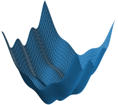
As an example, consider the nonconvex function

$$f(x)=\frac{1}{n}\sum_{i=1}^{n}a_{i}(x_{i}^{2}+4b_{i}\sin^{2}(x_{i})):=f_{i}(x),$$ (38)

where $a_{i}>0$ and $1>b_{i}>0$ for $i=1,\ldots,n$, so that each $f_{i}$ satisfies the PL condition (see Karimi et al., (2016)). The function (38) is interpolated since $x^{*}=0$ is a global minima for each $f_{i}$. Furthermore $f_{i}$ is smooth since $|f_{i}^{\prime\prime}(x)|\leq 2a_{i}+6b_{i}$. By the above arguments, so does $f$ satisfy the PL condition. Thus by Theorem 4.7 we know that SGD converges linearly when applied to (38). To illustrate that such functions (38) are nonconvex, we have a surface plot for $n=2$ in Figure 1.

Nonlinear least squares.

Let $F:\mathbb{R}^{d}\rightarrow\mathbb{R}^{n}$ be a differentiable function where $DF(x)\in\mathbb{R}^{n\times d}$ is its Jacobian. Now consider the nonlinear least squares problem $\min_{x\in\mathbb{R}^{d}}f(x):=\frac{1}{2n}\left\|F(x)-y\right\|^{2}=\frac{1}{2n}\sum_{i=1}^{n}(F_{i}(x)-y_{i})^{2},$ where $y\in\mathbb{R}^{n}.$

Lemma 5.2.

Assume there exists $x^{*}\in\mathbb{R}^{d}$ such that $F(x^{*})=y.$ If the $F_{i}(x)$ functions are Lipschitz and the $DF(x)$ has full row rank then $F$ satisfies the PL and the 3.1 condition.

Star/quasar-convex.

Several nonconvex empirical risk problems are quasar-convex functions (Lee and Valiant,, 2016). Let $f_{i}:\mathbb{R}^{d}\mapsto\mathbb{R}$ be a smooth star-convex (quasar-convex with $\zeta=1$) centered at $0$. Let ${\bf A}\in\mathbb{R}^{m\times n},b\in\mathbb{R}^{m}$ such that there exists ${\bf A}x^{*}=b.$ Since compositions of affine maps with star convex functions are star convex (Lee and Valiant,, 2016, Section A.4) we have that $f_{i}({\bf A}x-b)$ is star convex centered at $x^{*}.$ Furthermore the average of star convex functions that share the same center are star convex. Thus, $f(x)=\frac{1}{n}\sum_{i=1}^{n}f_{i}({\bf A}x-b),$ is a star-convex function which also satisfies the interpolation condition.

6 CONCLUSION

We establish a hierarchy between the expected residual (3.1) condition and a host of other assumptions previously used in the analysis of SGD in the smooth setting, showing that 3.1 is a strictly weaker condition. Using the 3.1, we present the first convergence results for SGD under different step-size selections (constant, decreasing, and stochastic Polyak step-size) on quasar-convex functions (4) without the bounded gradient or bounded variance assumption. For functions satisfying the PL condition (5) we provide tight theoretical convergence guarantees for minibatch SGD that recover the best-known convergence results for deterministic gradient descent and single-element sampling SGD as special cases, and all minibatch sizes in between.

Acknowledgements

Nicolas Loizou acknowledges support by the IVADO post-doctoral funding program.

The work of Othmane Sebbouh was supported in part by the French government under management of Agence Nationale de la Recherche as part of the ”Investissements d’avenir” program, reference ANR19-P3IA-0001 (PRAIRIE 3IA Institute). Othmane Sebbouh also acknowledges the support of a ”Chaire d’excellence de l’IDEX Paris Saclay”.

 

Supplementary Material
SGD for Structured Nonconvex Functions:
Learning Rates, Minibatching and Interpolation

 

The Supplementary Material is organized as follows: In Section A, we give some lemmas and consequences of smoothness. In Section B we present the proofs of the proposition, lemma and theorem related to the Expected Residual condition as presented in Section 3 of the main paper. In Section C we present the proofs of the main theorems. In Section D we provide additional convergence results under the strongly quasar-convex assumption (Section D.1), the Expected Smoothness assumption (Section D.2) and a minibatch analysis that does not rely on the interpolation condition (Section D.3).

Contents

1. 1 INTRODUCTION
   1. 1.1 Background and Main Contributions
   2. 1.2 SGD and Arbitrary Sampling
2. 2 CLASSES OF STRUCTURED NONCONVEX FUNCTIONS
3. 3 EXPECTED RESIDUAL (ER)
4. 4 CONVERGENCE ANALYSIS
   1. 4.1 Quasar Convex functions
      1. 4.1.1 Constant and Decreasing Step-sizes
      2. 4.1.2 Stochastic Polyak Step-size (SPS) - Guarantee Convergence without tuning
   2. 4.2 PL Condition
      1. 4.2.1 Constant Step-size
      2. 4.2.2 Decreasing Step-size
5. 5 EXAMPLES
6. 6 CONCLUSION
7. A Technical Lemmas on Smoothness
8. B Proofs of results on Expected Residual
   1. B.1 Proof of Lemma 3.2
   2. B.2 Proof of Proposition 3.3 and its expansion to all samplings.
   3. B.3 Proof of Theorem 3.4
9. C Proofs of Main Convergence Analysis Results
   1. C.1 Proof of Theorem 4.1
   2. C.2 Proof of Corollary 4.2
   3. C.3 Proof of Lemma 4.3
   4. C.4 Proof of Theorem 4.4
   5. C.5 Proof of Theorem 4.6
      1. C.5.1 Comparison of Theorem 4.6 to the PL Convergence Results by Khaled and Richtarik, (2020)
   6. C.6 Proof of Theorem 4.7
   7. C.7 Proof of Theorem 4.8
   8. C.8 Proofs of Section 5
      1. C.8.1 Proof of Theorem 5.1
      2. C.8.2 Separable, smooth and PL.
      3. C.8.3 Proof of Lemma 5.2
10. D Additional Convergence Analysis Results
    1. D.1 Convergence of SGD for Quasar Strongly Convex functions
       1. D.1.1 Constant Step-size
       2. D.1.2 Stochastic Polyak Step-size (SPS)
    2. D.2 Convergence Analysis Results under Expected Smoothness
       1. D.2.1 Quasar-Convex and Expected Smoothness
       2. D.2.2 PL and Expected Smoothness.
    3. D.3 Minibatch Corollaries without Interpolation
       1. D.3.1 Quasar Convex
       2. D.3.2 PL Function

Appendix A Technical Lemmas on Smoothness

Here we give some lemmas and consequences of smoothness.

For all of our analysis we do not need that the $f_{i}$ functions be smooth in all directions. Rather, we just need them to be smooth along the $x^{*}$–direction, as we define next.

Definition A.1.

We say that $f:\mathbb{R}^{d}\mapsto\mathbb{R}$ is $L$–smooth function along the $x^{*}$–direction if there exists $x^{*}$ such that

$$f(z)-f(x) \leq\left<\nabla f(x),z-x\right>+\frac{L}{2}\left\|z-x\right\|^{2},\quad\forall x\in\mathbb{R}^{d},$$ (39)

where

$$z=x-\frac{1}{L}(\nabla f(x)-\nabla f(x^{*})).$$

By inserting $z$ into (39) we can equivalently write (39) as

$$f\big{(}x-(1/L)(\nabla f(x)-\nabla f(x^{*}))\big{)}\leq f(x)-\frac{1}{2L}\left\|\nabla f(x)\right\|^{2}+\frac{1}{2L}\left\|\nabla f(x^{*})\right\|^{2}.$$ (40)

Lemma A.2.

Let $f:\mathbb{R}^{d}\mapsto\mathbb{R}$ be differentiable and suppose $f$ has a minimizer $x^{*}\in\mathbb{R}^{d}.$ Furthermore, let $f$ be $L$–smooth function along the $x^{*}$–direction according to Definition A.1. It follows that

$$\left\|\nabla f(x)\right\|^{2}\leq 2L(f(x)-f(x^{*})).$$ (41)

Proof.

Since $x^{*}$ is a minimizer of $f$ we have that $\nabla f(x^{*})=0.$ Furthermore, since $f$ is $L$–smooth function along the $x^{*}$–direction we have by re-arranging (40) that

$$f(x^{*})-f(x)\leq f\big{(}x-(1/L)\nabla f(x)\big{)}-f(x)\overset{\eqref{eq:smoothnessfuncstar2}}{\leq}-\frac{1}{2L}\left\|\nabla f(x)\right\|^{2}.$$

Re-arranging the above gives (41). ∎

Now we provide a lemma that will then be used to establish the simplest and most minimalistic assumptions that imply the expected residual (3.1) condition (Assumption 3.1).

Lemma A.3.

Suppose these exists $x^{*}\in\mathbb{R}^{d}$ where

$$x^{*}\in\operatorname{arg\,min}\left\{f(x):=\frac{1}{n}\sum_{i=1}f_{i}(x)\right\},$$

such that each $f_{i}$ is convex around $x^{*}$, that is

$$f_{i}(x^{*})-f_{i}(x) \leq\left<\nabla f_{i}(x^{*}),x^{*}-x\right>,\quad\forall x\in\mathbb{R}^{d},$$ (42)

and each $f_{i}$ is $L_{i}$–smooth along the $x^{*}$–direction according Definition A.1. It follows for every $i\in\{1,\ldots,n\}$ that

$$\left\|\nabla f_{i}(x)-\nabla f_{i}(x^{*})\right\|^{2}\leq 2L_{i}(f_{i}(x)-f_{i}(x^{*})-\left<\nabla f_{i}(x^{*}),x-x^{*}\right>),\quad\forall x\in\mathbb{R}^{d}.$$ (43)

Proof.

Fix $i\in\{1,\ldots,n\}$. To prove (43), it follows that

$$f_{i}(x^{*})-f_{i}(x) = f_{i}(x^{*})-f_{i}(z)+f_{i}(z)-f_{i}(x)$$ (44)

$$\overset{\eqref{eq:conv}+\eqref{eq:smoothnessfuncstar}}{\leq} \left<\nabla f_{i}(x^{*}),x^{*}-z\right>+\left<\nabla f_{i}(x),z-x\right>+\frac{L_{i}}{2}\left\|z-x\right\|^{2},$$

where

$$z=x-\frac{1}{L_{i}}(\nabla f_{i}(x)-\nabla f_{i}(x^{*})).$$ (45)

Substituting this in $z$ into (44) gives

$$f_{i}(x^{*})-f_{i}(x) = \left<\nabla f_{i}(x^{*}),x^{*}-x+\frac{1}{L_{i}}(\nabla f_{i}(x)-\nabla f_{i}(x^{*}))\right>-\frac{1}{L_{i}}\left<\nabla f_{i}(x),\nabla f_{i}(x)-\nabla f_{i}(x^{*})\right>$$

$$\quad+\frac{1}{2L_{i}}\left\|\nabla f_{i}(x)-\nabla f_{i}(x^{*})\right\|^{2}$$

$$= \left<\nabla f_{i}(x^{*}),x^{*}-x\right>-\frac{1}{L_{i}}\left\|\nabla f_{i}(x)-\nabla f_{i}(x^{*})\right\|^{2}+\frac{1}{2L_{i}}\left\|\nabla f_{i}(x)-\nabla f_{i}(x^{*})\right\|^{2}$$

$$= \left<\nabla f_{i}(x^{*}),x^{*}-x\right>-\frac{1}{2L_{i}}\left\|\nabla f_{i}(x)-\nabla f_{i}(x^{*})\right\|^{2}.$$

∎

Now we present a corollary of the previous lemma for over-parametrized functions We now develop an immediate consequence of each $f_{i}$ being convex around $x^{*}$ and smooth along the $x^{*}$– direction.

Corollary A.4.

Suppose these exists $x^{*}\in\mathbb{R}^{d}$ where

$$x^{*}\in\operatorname{arg\,min}\left\{f(x):=\frac{1}{n}\sum_{i=1}f_{i}(x)\right\}.$$

Suppose the interpolated Assumption 2.3 holds. Furthermore, suppose that for each $f_{i}$ there exists $L_{i}$ such that

$$f_{i}\left(x-\frac{1}{L_{i}}\nabla f_{i}(x)\right)\leq f_{i}(x)-\frac{1}{2L_{i}}\left\|\nabla f_{i}(x)\right\|^{2}.$$ (46)

It follows for every $i\in\{1,\ldots,n\}$ that

$$\left\|\nabla f_{i}(x)-\nabla f_{i}(x^{*})\right\|^{2}\leq 2L_{i}(f_{i}(x)-f_{i}(x^{*})).\quad\forall x\in\mathbb{R}^{d}.$$ (47)

Proof.

Note that for interpolated functions we have that each $f_{i}$ is convex around $x^{*}$. Furthermore, since each $\nabla f_{i}(x^{*})=0$ we have that (40) holds, and thus $f_{i}$ is smooth in the $x^{*}$–direction according to Definition A.1. Finally all the conditions of Lemma A.3 holds, and thus so does (47) holds. ∎

Appendix B Proofs of results on Expected Residual

B.1 Proof of Lemma 3.2

Proof.

Using

$$\left\|g(x)-\nabla f(x)\right\|^{2} \leq 2\left\|g(x)-g(x^{*})-\nabla f(x)\right\|^{2}+2\left\|g(x^{*})\right\|^{2},$$

and taking expectation together with (3.1) and $\nabla f(x^{*})=0$ gives

$${\mathbb{E}\left[\left\|g(x)-\nabla f(x)\right\|^{2}\right]} \leq 4\rho(f(x)-f(x^{*}))+2{\mathbb{E}_{{\cal D}}\left[\left\|g(x^{*})\right\|^{2}\right]}.$$

Taking the supremum over $x^{*}\in{\cal X}^{*}$ and using  Assumption 1.2 and that ${\mathbb{E}\left[\left\|X-{\mathbb{E}\left[X\right]}\right\|^{2}\right]}={\mathbb{E}\left[\left\|X\right\|^{2}\right]}-\left\|{\mathbb{E}\left[X\right]}\right\|^{2}$ with $X=g(x)$ gives (7). ∎

B.2 Proof of Proposition 3.3 and its expansion to all samplings.

In this section we give an expanded version of Proposition 3.3 that also gives bounds for the Expected Smoothness assumption (ES), a closely related assumption to the Expected Residual condition.

Assumption B.1 (Expected smoothness).

We say that the stochastic gradient $g$ satisfy the expected smoothness assumption if for all $x\in\mathbb{R}^{d}$, there exists ${\cal L}={\cal L}(g)>0$ such that

$${\mathbb{E}_{{\cal D}}\left[\left\|g(x)-g(x^{*})\right\|^{2}\right]}\leq 2{\cal L}\left(f(x)-f(x^{*})\right).$$ (ES)

We use $g\in\text{ES}({\cal L})$ as shorthand for expected smoothness.

Here we show that a sufficient condition for the expected smoothness and the expected residual conditions B.1 and 3.1 to hold if that each $f_{i}$ is convex around $x^{*}$ and smooth. Furthermore, we give tight bounds on the expected smoothness ${\cal L}$ and the expected residual constant $\rho$ for when $v$ is an independent sampling and, in particular, a $b$–minibatch sampling.

In the main text our minibatch results are stated only for $b$–minibatching. But they actually hold for a large family of sampling that we refer to as the independent samplings.

Definition B.2 (Independent sampling).

Let $S\subset\{1,\ldots,n\}$ be a random set and let let $v=\sum_{i\in S}\frac{1}{p_{i}}e_{i}$ which is a sampling vector. Suppose there exists a constant $c_{2}>0$ such that

$$\frac{\mathbb{P}\left[i,j\in S\right]}{\mathbb{P}\left[i\in S\right]\mathbb{P}\left[j\in S\right]}=c_{2},\quad\forall i,j\in\{1,\ldots,n\},\;i\neq j.$$ (48)

In Gower et al., (2019) it was proven that an independent sampling vector is indeed a valid sampling vector. For completeness we also give the proof in In Lemma C.2. Furthermore, all the samplings presented in Gower et al., (2019) are examples of an independent sampling vector. In particular the minibatch sampling in Definition 1.1 is also an independent sampling. Finally, note that (48) does not imply that $i\in S$ and $j\in S$ are independent events unless $c_{2}=1.$ Indeed, for $b$–minibatch sampling we have that $\mathbb{P}\left[i\in S\right]=\frac{b}{n}=\mathbb{P}\left[j\in S\right]$ and $\mathbb{P}\left[i,j\in S\right]=\frac{b}{n}\frac{b-1}{n-1}$ and thus they are not independent events yet satisfy (48) with $c_{2}=\frac{n}{b}\frac{b-1}{n-1}.$

The following Proposition is based on the proof of Proposition 3.8 in Gower et al., (2019) with the exception that now we show that only convexity around $x^{*}$ is required for the proof to follow, as opposed to assuming convexity everywhere.

Proposition B.3.

Let $f$ be a finite sum problem $f=\frac{1}{n}\sum_{i=1}^{n}f_{i}$. Let $f_{i}$ be $L_{i}$–smooth and convex around $x^{*}$ according to (A.1) and (42), respectively. It follows that

1. If $v$ is a sampling vector then the expected smoothness and expected residual conditions hold $g\in\text{ES}({\cal L})$ and $g\in\text{ER}(\rho)$ with ${\cal L}=\max_{v}\frac{1}{n}\sum_{i=1}^{n}L_{i}v_{i}=\rho.$

2. If $v$ is an independent sampling vector according to Definition B.2 then we have that

   $${\cal L} =c_{2}L+\max_{i=1,\ldots,n}\frac{L_{i}}{np_{i}}\left(1-p_{i}c_{2}\right).$$ (49)

   $$\rho =\frac{\lambda_{\max}({\mathbb{E}\left[(v-\mathbf{1})(v-\mathbf{1})^{\top}\right]})}{n}L_{\max}$$ (50)

3. If $v$ is the $b$–minibatch sampling with replacement then

   $$\sigma^{2} =\frac{1}{b}\frac{n-b}{n-1}\sigma_{1}^{2}$$ (51)

   $$\rho =\frac{1}{b}\frac{n-b}{n-1}L_{\max}$$ (52)

   $${\cal L} =\frac{n}{b}\frac{b-1}{n-1}L+\frac{1}{b}\frac{n-b}{n-1}L_{\max}.$$ (53)

Proof.

1. Assume that $v$ is any sampling vector. Since $f_{i}$ is $L_{i}$–smooth and convex around $x^{*}$ we have that by multiplying each side of

   $$f_{i}(z)-f_{i}(x) \leq\left<\nabla f_{i}(x),z-x\right>+\frac{L_{i}}{2}\left\|z-x\right\|^{2}$$

   $$f_{i}(x^{*})-f_{i}(x) \leq\left<\nabla f_{i}(x^{*}),x^{*}-x\right>,$$

   by $v_{i}/n$ and summing up over $i=1,\ldots,n$ bearing in mind that $v_{i}\geq 0$ we have that

   $$f_{v}(z)-f_{v}(x) \leq\left<\nabla f_{v}(x),z-x\right>+\frac{\frac{1}{n}\sum_{i=1}^{n}v_{i}L_{i}}{2}\left\|z-x\right\|^{2}$$

   $$f_{v}(x^{*})-f_{v}(x) \leq\left<\nabla f_{v}(x^{*}),x^{*}-x\right>.$$

   Consequently $f_{v}$ is convex and $x^{*}$ and is $L_{v}$–smooth where $L_{v}:=\frac{1}{n}\sum_{i=1}^{n}v_{i}L_{i}$. Applying Lemma A.3 we thus have that

   $$\left\|\nabla f_{v}(x)-\nabla f_{v}(x^{*})\right\|^{2}\leq L_{v}(f_{v}(x)-f_{v}(x^{*})-\left<\nabla f_{v}(x^{*}),x-x^{*}\right>),\quad\forall x\in\mathbb{R}^{d}.$$ (54)

   Taking expectation gives

   $${\mathbb{E}\left[\left\|\nabla f_{v}(x)-\nabla f_{v}(x^{*})\right\|^{2}\right]} \leq{\mathbb{E}\left[L_{v}(f_{v}(x)-f_{v}(x^{*})-\left<\nabla f_{v}(x^{*}),x-x^{*}\right>)\right]}$$

   $$\leq\max_{v}L_{v}{\mathbb{E}\left[(f_{v}(x)-f_{v}(x^{*})-\left<\nabla f_{v}(x^{*}),x-x^{*}\right>)\right]}$$

   $$=\max_{v}L_{v}(f(x)-f(x^{*})).$$

   This proves that the expected smoothness assumption holds with ${\cal L}=\max_{v}L_{v}.$ Consequently by Theorem 3.4 we have that the expected residual condition holds with $\rho={\cal L}.$

2. Assume that $v_{i}$ is an independent sampling. First we prove (49).

   Since $f_{i}$ is $L_{i}$–smooth and convex around $x^{*}$ we have that $f$ is $L$–smooth and convex around $x^{*}$ and by Lemma A.3

   $$\|\nabla f_{i}(x)-\nabla f_{i}(x^{*})\|^{2}\leq 2L_{i}(f_{i}(x)-f_{i}(x^{*})-\langle\nabla f_{i}(x^{*}),x-x^{*}\rangle)$$ (55)

   $$\|\nabla f(x)-\nabla f(x^{*})\|^{2}\leq 2L(f(x)-f(x^{*})-\langle\nabla f(x^{*}),x-x^{*}\rangle).$$ (56)

   Noticing that

   $$\|\nabla f_{v}(x)-\nabla f_{v}(x^{*})\|^{2} = \frac{1}{n^{2}}\left\|\sum_{i\in S}\frac{1}{p_{i}}(\nabla f_{i}(x)-\nabla f_{i}(x^{*}))\right\|^{2}$$

   $$= \sum_{i,j\in S}\left\langle\frac{1}{np_{i}}(\nabla f_{i}(x)-\nabla f_{i}(x^{*})),\frac{1}{np_{j}}(\nabla f_{j}(x)-\nabla f_{j}(x^{*}))\right\rangle,$$

   we have

   $$\mathbb{E}[\|\nabla f_{v}(x)-\nabla f_{v}(x^{*})\|^{2}] = \sum_{C}p_{C}\sum_{i,j\in C}\left\langle\frac{1}{np_{i}}(\nabla f_{i}(x)-\nabla f_{i}(x^{*})),\frac{1}{np_{j}}(\nabla f_{j}(x)-\nabla f_{j}(x^{*}))\right\rangle$$

   $$= \sum_{i,j=1}^{n}\sum_{C:i,j\in C}p_{C}\left\langle\frac{1}{np_{i}}(\nabla f_{i}(x)-\nabla f_{i}(x^{*})),\frac{1}{np_{j}}(\nabla f_{j}(x)-\nabla f_{j}(x^{*}))\right\rangle$$

   $$= \sum_{i,j=1}^{n}\frac{\mathbb{P}\left[i,j\in S\right]}{p_{i}p_{j}}\left\langle\frac{1}{n}(\nabla f_{i}(x)-\nabla f_{i}(x^{*})),\frac{1}{n}(\nabla f_{j}(x)-\nabla f_{j}(x^{*}))\right\rangle,$$

   where we used a double counting argument in the 2nd equality. Now since $\mathbb{P}\left[i,j\in S\right]/(p_{i}p_{j})=c_{2}$ for $i\neq j.$ Recalling that $\mathbb{P}\left[i,i\in S\right]=p_{i}$ we have from the above that

   $$\mathbb{E}[\|\nabla f_{v}(x)-\nabla f_{v}(x^{*})\|^{2}] = \sum_{i\neq j}c_{2}\left\langle\frac{1}{n}(\nabla f_{i}(x)-\nabla f_{i}(x^{*})),\frac{1}{n}(\nabla f_{j}(x)-\nabla f_{j}(x^{*}))\right\rangle$$

   $$\qquad+\sum_{i=1}^{n}\frac{1}{n^{2}}\frac{1}{p_{i}}\left\|\nabla f_{i}(x)-\nabla f_{i}(x^{*}))\right\|^{2}$$

   $$= \sum_{i,j=1}^{n}c_{2}\left\langle\frac{1}{n}(\nabla f_{i}(x)-\nabla f_{i}(x^{*})),\frac{1}{n}(\nabla f_{j}(x)-\nabla f_{j}(x^{*}))\right\rangle$$

   $$+\sum_{i=1}^{n}\frac{1}{n^{2}}\frac{1}{p_{i}}\left(1-p_{i}c_{2}\right)\left\|\nabla f_{i}(x)-\nabla f_{i}(x^{*}))\right\|^{2}$$

   $$\overset{\eqref{eq:procL1}}{\leq} c_{2}\left\|\nabla f(x)-\nabla f(x^{*})\right\|^{2}$$

   $$+2\sum_{i=1}^{n}\frac{1}{n^{2}}\frac{L_{i}}{p_{i}}\left(1-p_{i}c_{2}\right)(f_{i}(x)-f_{i}(x^{*})-\langle\nabla f_{i}(x^{*}),x-x^{*}\rangle)$$

   $$\overset{\eqref{eq:procL2}}{\leq} 2\left(c_{2}L+\max_{i=1,\ldots,n}\frac{L_{i}}{np_{i}}\left(1-p_{i}c_{2}\right)\right)(f(x)-f(x^{*})-\langle\nabla f(x^{*}),x-x^{*}\rangle).$$

   Comparing the above to the definition of expected smoothness (ES) we have that

   $${\cal L}\quad\leq\quad c_{2}L+\max_{i=1,\ldots,n}\frac{L_{i}}{np_{i}}\left(1-p_{i}c_{2}\right).$$ (57)

   Now we will prove that

   $${\mathbb{E}\left[\left\|\nabla f_{v}(w)-\nabla f_{v}(x^{*})-(\nabla f(w)-\nabla f(x^{*}))\right\|^{2}\right]}\leq 2\rho\left(f(w)-f(x^{*})\right),$$ (58)

   holds with the constant given in (50). First we expand the squared norm on the left hand side of (58). Define $DF(w)=[\nabla f_{1}(w),\ldots,\nabla f_{n}(w)]\in\mathbb{R}^{d\times n}$ as the Jacobian of $F(w)\overset{def}{=}[f_{1}(w),\dots,f_{n}(w)]$. We denote ${\bf R}:=\left(DF(w)-DF(x^{*})\right)$. It follows that

   $$C :=\left\|\nabla f_{v}(w)-\nabla f_{v}(x^{*})-(\nabla f(w)-\nabla f(x^{*}))\right\|^{2}$$

   $$=\frac{1}{n^{2}}\left\|\left(DF(w)-DF(x^{*})\right)(v-\mathbf{1})\right\|^{2}$$

   $$=\frac{1}{n^{2}}\langle{\bf R}(v-\mathbf{1}),{\bf R}(v-\mathbf{1})\rangle_{\mathbb{R}^{d}}$$

   $$=\frac{1}{n^{2}}{\rm Trace}\left((v-\mathbf{1})^{\top}{\bf R}^{\top}{\bf R}(v-\mathbf{1})\right)$$

   $$=\frac{1}{n^{2}}{\rm Trace}\left({\bf R}^{\top}{\bf R}(v-\mathbf{1})(v-\mathbf{1})^{\top}\right).$$

   Let $\mathbf{Var}\left[v\right]:={\mathbb{E}\left[(v-\mathbf{1})(v-\mathbf{1})^{\top}\right]}.$ Taking expectation,

   $${\mathbb{E}\left[C\right]} = \frac{1}{n^{2}}{\rm Trace}\left({\bf R}^{\top}{\bf R}\mathbf{Var}\left[v\right]\right)$$ (59)

   $$\leq \frac{1}{n^{2}}{\rm Trace}\left({\bf R}^{\top}{\bf R}\right)\lambda_{\max}(\mathbf{Var}\left[v\right]).$$

   Moreover, since the $f_{i}$’s are convex around $x^{*}$ and $L_{i}$-smooth, it follows from (43) that

   $${\rm Trace}\left({\bf R}^{\top}{\bf R}\right) = \sum_{i=1}^{n}\left\|\nabla f_{i}(w)-\nabla f_{i}(x^{*})\right\|^{2}$$ (60)

   $$\leq 2\sum_{i=1}^{n}L_{i}(f_{i}(w)-f_{i}(x^{*})-\langle\nabla f_{i}(x^{*}),w-x^{*}\rangle)$$

   $$\leq 2nL_{\max}(f(w)-f(x^{*})).$$

   Therefore,

   $${\mathbb{E}\left[C\right]}\overset{\eqref{eq:trace-eig}+\eqref{eq:traceRtT}}{\leq}2\frac{\lambda_{\max}(\mathbf{Var}\left[v\right])}{n}L_{\max}(f(w)-f(x^{*})).$$ (61)

   Which means

   $$\rho=\frac{\lambda_{\max}(\mathbf{Var}\left[v\right])}{n}L_{\max}.$$ (62)

3. Finally, if $v$ is a $b$–minibatch sampling, the specialized expressions for ${\cal L}$ in (53) follows by observing that $\mathbb{P}\left[i\in S\right]=p_{i}=\frac{b}{n}$, $\mathbb{P}\left[i,j\in S\right]=\frac{b}{n}\frac{b-1}{n-1}$ and consequently $c_{2}=\frac{n}{b}\frac{b-1}{n-1}.$ The specialized expressions for $\sigma$ and $\rho$ in (51) and (52) follow from Proposition 3.8 Gower et al., (2019) and Lemma F.3 in Sebbouh et al., (2019), respectively.

∎

B.3 Proof of Theorem 3.4

First we include the formal definition of each of these assumptions named in Theorem 3.4. Let $g(x)=\nabla f_{i}(x)$ denote the stochastic gradient. The results in this section carry over verbatim by using $g(x)=\nabla f_{v}(x)$ and $f_{i}=f_{v}$ instead, where $v$ is a sampling vector. But since the sampling only affects the constants in each of the forthcoming assumptions, and here we are only interested in a hierarchy between assumptions, we omit the proof for a general sampling vector.

First we repeat the definitions of $ES$, $WGC$ and $SGC$ from Assumption 2 Khaled and Richtarik, (2020), Assumption 2.1 in Gower et al., (2019), Eq (7) and Eq (2) in Vaswani et al., 2019a , respectively.

SGC: Strong Growth Condition.

We say that $SGC$ holds with $\rho_{SGC}>0$ if

$${\mathbb{E}\left[\left\|g(x)\right\|^{2}\right]}\leq\rho_{SGC}\left\|\nabla f(x)\right\|^{2}.$$ (63)

WGC: Weak Growth Condition.

We say that $WGC$ holds with $\rho_{WGC}>0$ if

$${\mathbb{E}\left[\left\|g(x)\right\|^{2}\right]}\leq 2\rho_{WGC}(f(x)-f(x^{*})).$$ (64)

ES: Expected Smoothness.

We say that $ES$ holds with ${\cal L}>0$ if

$${\mathbb{E}\left[\left\|g(x)-g(x^{*})\right\|^{2}\right]}\leq 2{\cal L}(f(x)-f(x^{*})).$$ (65)

ER: Expected Residual.

We say that $ER$ holds with $\rho>0$ if

$${\mathbb{E}\left[\left\|g(x)-g(x^{*})-(\nabla f(x)-\nabla f(x^{*}))\right\|^{2}\right]}\leq 2\rho\left(f(x)-f(x^{*})\right).$$ (66)

In addition we will use

$x^{*}$–convex.

We say that $x^{*}$–convex holds if

$$f_{i}(x^{*})-f_{i}(x)\leq\left<\nabla f_{i}(x^{*}),x^{*}-x\right>,\quad\mbox{for }i=1,\ldots,n.$$ (67)

$L_{i}$–smoothness.

We say that $L_{i}$–smoothness holds for $L_{i}>0$ if

$$f_{i}(z)-f_{i}(x)\leq\left<\nabla f_{i}(x),z-x\right>+\frac{L_{i}}{2}\left\|z-x\right\|^{2},\quad\forall x,z\in\mathbb{R}^{d},\;i=1,\ldots,n.$$ (68)

Interpolated.

We say that the interpolation condition holds at $x^{*}$ if

$$f_{i}(x^{*})\leq f_{i}(x),\quad\mbox{for }i=1,\ldots,n,\mbox{and for every }x\in\mathbb{R}^{d}.$$ (69)

An important assumption created recently Khaled and Richtarik, (2020) is the following $ABC$–assumption

ABC.

We say that $ABC$ holds with $A,B,C>0$ if

$${\mathbb{E}\left[\left\|g(x)\right\|^{2}\right]}\leq 2A(f(x)-f(x^{*})+B\left\|\nabla f(x)\right\|^{2}+C.$$ (70)

The $ABC$ condition (70) includes all previous assumptions SGC, WGC, ES and ER as a special case by choosing the three parameters $A,B$ and $C$ appropriately. In this sense, it is a family of assumptions. See Khaled and Richtarik, (2020) for more details on this assumption and how it linked to all the other assumptions.

Now we repeat the statement of Theorem 3.4 for convenience.

Theorem B.4.

The following hierarchy holds

$${\begin{array}[c]{cccccccccccc}\boxed{SGC+L\mbox{--smooth}}&\Longrightarrow&\boxed{WGC}&\Longrightarrow&\boxed{ES}&\Longrightarrow&\boxed{\hbox{\pagecolor{blue!20}ER}}&\Longrightarrow&ABC\\ &&&&\Uparrow&&&&\\ &&\boxed{L_{i}+\mbox{Interpolated}}&\Longrightarrow&\boxed{L_{i}+x^{*}\mbox{--convex}}&&\end{array}}$$

In addition we have that $ES({\cal L})+PL(\mu)\Rightarrow ER({\cal L}-\mu)$ and $ER\nRightarrow ES.$

Proof.

We first prove the top row of implications.
 1. $SGC+L\mbox{--smooth}\implies WGC$. Using Lemma A.2 and (63) we have that

$${\mathbb{E}\left[\left\|g(x)\right\|^{2}\right]} \leq \rho_{SGC}\left\|\nabla f(x)\right\|^{2}$$

$$\overset{\eqref{eq:smoothsubopt}}{\leq} 2L\rho_{SGC}(f(x)-f(x^{*})).$$

Thus (64) holds with $\rho_{WGC}=2L\rho_{SGC}.$

2. $WGC\implies ES$.

Plugging in $x=x^{*}$ in WGC (64) gives $g(x^{*})=0$ almost surely. Since $g(x^{*})=0$ we have that  (64) gives (65).

3.$ES\implies ER$. Expanding the squares of the left hand side of (66) gives

$$\left\|g(x)-g(x^{*})-(\nabla f(x)-\nabla f(x^{*}))\right\|^{2} =\left\|g(x)-g(x^{*})\right\|^{2}+\left\|\nabla f(x)-\nabla f(x^{*})\right\|^{2}$$

$$\quad-2\left<g(x)-g(x^{*}),\nabla f(x)-\nabla f(x^{*})\right>.$$

Now assuming that $ES$ (65) holds, taking expectation and using that ${\mathbb{E}\left[g(x)\right]}=\nabla f(x)$ we have that

$${\mathbb{E}\left[\left\|g(x)-g(x^{*})-(\nabla f(x)-\nabla f(x^{*}))\right\|^{2}\right]} ={\mathbb{E}\left[\left\|g(x)-g(x^{*})\right\|^{2}\right]}-\left\|\nabla f(x)-\nabla f(x^{*})\right\|^{2}$$

$$\leq{\mathbb{E}\left[\left\|g(x)-g(x^{*})\right\|^{2}\right]}$$

$$\leq 2{\cal L}(f(x)-f^{*}).$$

In addition, if the PL condition holds, then we can upper bound $-\left\|\nabla f(x)-\nabla f(x^{*})\right\|^{2}\leq-2\mu(f(x)-f^{*})$ which combined with the above gives

$${\mathbb{E}\left[\left\|g(x)-g(x^{*})-(\nabla f(x)-\nabla f(x^{*}))\right\|^{2}\right]}\leq 2({\cal L}-\mu)(f(x)-f^{*}).$$

Thus $ER$ holds with $\rho={\cal L}-\mu.$

Now we prove the remaining implications.

4. $L_{i}+$Interpolated $\implies L_{i}+x^{*}\mbox{--convex}$. A direct consequence of the interpolation assumption (2.3) is that $\nabla f_{i}(x^{*})=0$ and $f_{i}(x^{*})\leq f_{i}(x).$ Consequently $f_{i}(x^{*})\leq f_{i}(x)+\left<\nabla f_{i}(x^{*}),x-x^{*}\right>$.

5. $L_{i}+x^{*}\mbox{--convex}\implies ES$. Follows from Proposition B.3.

6. $ER\nRightarrow ES$. Since when $v$ encodes the full batch sampling where $g(x)=\nabla f(x)$, the expected residual condition always holds for any $\rho>0$ since the left hand side of (3.1) is zero and $0\leq\rho(f(x)-f^{*}).$ On the other hand, in the full batch case the expected smoothness assumption is equivalent to claiming that $f$ is $L$–smooth, and clearly there exist differentiable functions that have gradients that are not Lipschitz. For instance $f(x)=x^{4}.$

Finally
7. $ER\Rightarrow ABC$. If the ER condition holds, by Lemma 3.2 we have that (7) holds, which fits the format of the ABC assumption (70) where $A=2\rho$, $B=1$ and $C=2\sigma^{2}.$ ∎

Appendix C Proofs of Main Convergence Analysis Results

C.1 Proof of Theorem 4.1

First we need the following lemma.

Lemma C.1.

Assume $g\in ER(\rho)$. Then for all $x\in\mathbb{R}^{d}$,

$${\mathbb{E}_{{\cal D}}\left[\left\|g(x)\right\|^{2}\right]}\leq 2(2\rho+L)(f(x)-f(x^{*})+2\sigma^{2}.$$ (71)

Proof.

Since $f$ is $L-$smooth, we have $\left\|\nabla f(x)\right\|^{2}\leq 2L(f(x)-f(x^{*})).$ Using this inequality together with (7) gives (71). ∎

Proof.

We have:

$$\left\|x^{k+1}-x^{*}\right\|^{2} =\left\|x^{k}-x^{*}\right\|^{2}-2\gamma_{k}\langle g(x^{k}),x^{k}-x^{*}\rangle+\gamma_{k}^{2}\left\|g(x^{k})\right\|^{2}$$

Hence, taking expectation conditioned on $x_{k}$, we have:

$${\mathbb{E}_{{\cal D}}\left[\left\|x^{k+1}-x^{*}\right\|^{2}\right]} = \left\|x^{k}-x^{*}\right\|^{2}-2\gamma_{k}\langle\nabla f(x^{k}),x^{k}-x^{*}\rangle+\gamma_{k}^{2}{\mathbb{E}_{{\cal D}}\left[\left\|\nabla f_{v_{k}}(x_{k})\right\|^{2}\right]}$$

$$\overset{\eqref{eq:quasar-convex}+\eqref{eq:varbndrho3}}{\leq} \left\|x^{k}-x^{*}\right\|-2\gamma_{k}(\zeta-\gamma_{k}(2\rho+L))(f(x^{k})-f^{*}))+2\gamma_{k}^{2}\sigma^{2}.$$

Rearranging and taking expectation, we have

$$2\gamma_{k}(\zeta-\gamma_{k}(2\rho+L)){\mathbb{E}\left[f(x^{k})-f^{*}\right]}\leq{\mathbb{E}\left[\left\|x^{k}-x^{*}\right\|^{2}\right]}-{\mathbb{E}\left[\left\|x^{k+1}-x^{*}\right\|^{2}\right]}+2\gamma_{k}^{2}\sigma^{2}.$$

Summing over $k=0,\ldots,t-1$ and using telescopic cancellation gives

$$2\sum_{k=0}^{t-1}\gamma_{k}(\zeta-\gamma_{k}(2\rho+L)){\mathbb{E}\left[f(x_{k})-f^{*}\right]}\leq\left\|x^{0}-x^{*}\right\|^{2}-{\mathbb{E}\left[\left\|x^{k}-x^{*}\right\|^{2}\right]}+2\sigma^{2}\sum_{k=0}^{t-1}\gamma_{k}^{2}.$$

Since ${\mathbb{E}\left[\left\|x^{k}-x^{*}\right\|^{2}\right]}\geq 0$ and $(\zeta-\gamma_{k}(2\rho+L))\geq 0$, dividing both sides by $2\sum_{i=0}^{t-1}\gamma_{i}(\zeta-\gamma_{i}(2\rho+L))$ gives:

$$\sum_{k=0}^{t-1}{\mathbb{E}\left[\frac{\gamma_{k}(\zeta-\gamma_{k}(2\rho+L)}{\sum_{i=0}^{t-1}\gamma_{i}(\zeta-\gamma_{i}(2\rho+L))}(f(x^{k})-f^{*})\right]}\leq\frac{\left\|x^{0}-x^{*}\right\|^{2}}{2\sum_{i=0}^{t-1}\gamma_{i}(\zeta-\gamma_{i}(2\rho+L))}+\frac{\sigma^{2}\sum_{k=0}^{t-1}\gamma_{k}^{2}}{\sum_{i=0}^{t-1}\gamma_{i}(\zeta-\gamma_{i}(2\rho+L))}.$$

Thus,

$$\min_{k=0,\dots,t-1}{\mathbb{E}\left[f(x^{k})-f(x^{*})\right]}\leq\frac{\left\|x^{0}-x^{*}\right\|^{2}}{2\sum_{i=0}^{t-1}\gamma_{i}(\zeta-\gamma_{i}(2\rho+L))}+\frac{\sigma^{2}\sum_{k=0}^{t-1}\gamma_{k}^{2}}{\sum_{i=0}^{t-1}\gamma_{i}(\zeta-\gamma_{i}(2\rho+L))}.$$

For the different choices of step sizes:

1. If $\forall k\in\mathbb{N},\;\gamma_{k}=\frac{1}{2}\frac{\zeta}{(2\rho+L)}$, then it suffices to replace $\gamma_{k}=\gamma$ in (15).

2. Suppose algorithm (3) is run for $T$ iterations. Let $\forall k=0,\dots,T-1,\;\gamma_{k}=\frac{\gamma}{\sqrt{T}}$ with $\gamma\leq\frac{\zeta}{2(2\rho+L)}$. Notice that since $\gamma\leq\frac{\zeta}{2(2\rho+L)}$, we have $\zeta-\gamma(2\rho+L)\leq\frac{1}{2}$. Then it suffices to replace $\gamma_{k}=\frac{\gamma}{\sqrt{T}}$ in (15).

3. Let $\forall k\in\mathbb{N},\;\gamma_{k}=\frac{\gamma}{\sqrt{k+1}}$ with $\gamma\leq\frac{\zeta}{2\rho+L}$. Note that that since $\gamma_{t}=\frac{\gamma}{\sqrt{t+1}}$ and using the integral bound, we have that

   $$\sum_{t=0}^{k-1}\gamma_{t}^{2}=\gamma^{2}\sum_{t=0}^{k-1}\frac{1}{t+1}\;\leq\;\gamma^{2}\left(\log(k)+1\right).$$ (72)

   Furthermore using the integral bound again we have that

   $$\sum_{t=0}^{k-1}\gamma_{t} \geq 2\gamma\left(\sqrt{k}-1\right).$$ (73)

   Now using (72) and (73) we have that

   $$\sum_{i=0}^{k-1}\gamma_{i}(\zeta-\gamma_{i}(2\rho+L)) = \zeta\sum_{i=0}^{k-1}\gamma_{i}-(2\rho+L)\sum_{i=0}^{k-1}\gamma_{i}^{2}$$

   $$\geq 2\gamma\left(\zeta(\sqrt{k}-1)-\gamma(\rho+\frac{L}{2})\left(\log(k)+1\right)\right).$$

   It remains to replace bound the sums in (15) by the values we have computed.

∎

C.2 Proof of Corollary 4.2

Proof.

The interpolated assumption 2.3 implies that $\nabla f_{i}(x^{*})=g(x^{*})=0$ and thus $\sigma=0.$ Furthermore from (10) we have that the 3.1 condition holds with $\rho=L_{\max}\frac{n-b}{(n-1)b}$. Combining these two observations with (16) gives (4.2). The total complexity (20) follows from computing the iteration complexity via (4.2) and multiplying it by $b$.

Finally for the optimal minibatch size, since (20) is a linear function in $b$, the minimum depends on the sign of its slope. Taking the derivative in $b$ we have the slope is given by $2\frac{L-2L_{\max}}{n-1}$. If the slope is negative, we want $b$ to be a large as possible, that is $b=n$. Otherwise if the slope is positive $b=1$ is optimal. ∎

C.3 Proof of Lemma 4.3

Before presenting our proof for Lemma C.3, we need to present a large family of sampling vectors called the arbitrary samplings.

Lemma C.2 (Lemma 3.3  Gower et al., (2019)).

Let $S\subset\{1,\ldots,n\}$ be a random set. Let $\mathbb{P}\left[i\in S\right]=p_{i}$. It follows that $v=\sum_{i\in S}\frac{1}{p_{i}}e_{i}$ is a sampling vector. We call $v$ the arbitrary sampling vector.

An arbitrary sampling is sufficiently flexible as to model almost all samplings and minibatching schemes of interest, see Section 3.2 i nGower et al., (2019). For example the $b$–minibatch sampling is a special case where $p_{i}=\frac{b}{n}$ and $\mathbb{P}\left[S=B\right]=\left.1\right/\binom{n}{b}$ for every $B\in\{1,\ldots,n\}$ that has $b$ elements.

Now we prove Lemma 4.3 and some additional results.

Lemma C.3.

Assume interpolation 2.3 holds. Let $f_{i}$ be $L_{i}$–smooth and let $v$ be a sampling vector as defined in Lemma C.2. It follows that there exists ${\cal L}_{\max}>0$ such that

$$\frac{1}{2{\cal L}_{\max}}(f(x)-f^{*})\leq{\mathbb{E}\left[\frac{(f_{v}(x)-f_{v}^{*})^{2}}{\|\nabla f_{v}(x)\|^{2}}\right]}.$$ (74)

For $B\subset\{1,\ldots,n\}$ let $L_{B}$ be the smoothness constant of $f_{B}:=\frac{1}{n}\sum_{i\in B}p_{i}f_{i}$. It follows that
1. If $v$ is an arbitrary sampling vector (Lemma C.2) then ${\cal L}_{\max}=\underset{i=1,\ldots,n}{\max}\dfrac{p_{i}}{\sum_{B:i\in B}\frac{p_{B}}{L_{B}}}.$
2. If $v$ is the $b$–minibatch sampling then ${\cal L}_{\max}\;=\;{\cal L}_{\max}(b)\;=\;\underset{i=1,\ldots,n}{\max}\dfrac{\binom{n-1}{b-1}}{\sum_{B:i\in B}L_{B}^{-1}}.$

Proof.

Since $f_{i}$ is $L_{i}$–smooth, we have that $f_{v}$ is $L_{v}$–smooth with $L_{v}:=\frac{1}{n}\sum_{i=1}^{n}v_{i}L_{i}.$ Thus according to Lemma A.3 we have that

$$\|\nabla f_{v}(x)\|^{2}\leq 2L_{v}(f_{v}(x)-f_{v}^{*}).$$

Consequently we have that

$$\frac{1}{\|\nabla f_{v}(x)\|^{2}}\geq\frac{1}{2L_{v}(f_{v}(x)-f_{v}^{*})}.$$ (75)

Using this we have the following bound

$${\mathbb{E}\left[\frac{(f_{v}(x)-f_{v}^{*})^{2}}{\|\nabla f_{v}(x)\|^{2}}\right]}\overset{\eqref{eq:tempgradvbnd}}{\geq}{\mathbb{E}\left[\frac{f_{v}(x)-f_{v}^{*}}{2L_{v}}\right]}.$$ (76)

Let $S$ be the random set associated to the arbitrary sampling vector $v$. We use $B\subset\{1,\ldots,n\}$ to denote a realization of $S$ and $p_{B}:=\mathbb{P}\left[B=S\right].$ Thus with this notation we have that

$${\mathbb{E}\left[\frac{(f_{v}(x)-f_{v}^{*})^{2}}{\|\nabla f_{v}(x)\|^{2}}\right]} \overset{\eqref{eq:tempasdasda}}{\geq} \sum_{B\subset\{1,\ldots,n\}}p_{B}\frac{f_{B}(x)-f_{B}^{*}}{2L_{B}}.$$ (77)

Now let $p_{i}:=\mathbb{P}\left[i\in S\right].$ Due to the interpolation condition we have that and the definition of $f_{B}$ we have that

$$f_{B}^{*}=f_{B}(x^{*})=\frac{1}{n}\sum_{i\in B}p_{i}f_{i}(x^{*})=\frac{1}{n}\sum_{i\in B}p_{i}f_{i}^{*}.$$

Consequently

$${\mathbb{E}\left[\frac{(f_{v}(x)-f_{v}^{*})^{2}}{\|\nabla f_{v}(x)\|^{2}}\right]} \overset{\eqref{eq:tempsinejoise}}{=} \sum_{B\subset\{1,\ldots,n\}}p_{B}\sum_{i\in B}\frac{f_{i}(x)-f_{i}^{*}}{2nL_{B}p_{i}}$$ (78)

$$= \frac{1}{2n}\sum_{i=1,\ldots,n}\sum_{B:i\in B}\frac{p_{B}}{p_{i}L_{B}}(f_{i}(x)-f_{i}^{*})$$

$$\geq \min_{i=1,\ldots,n}\left\{\sum_{B:i\in B}\frac{p_{B}}{p_{i}L_{B}}\right\}\frac{1}{2cn}\sum_{i=1,\ldots,n}(f_{i}(x)-f_{i}^{*})$$

$$= \frac{1}{2}\min_{i=1,\ldots,n}\left\{\sum_{B:i\in B}\frac{p_{B}}{p_{i}L_{B}}\right\}(f(x)-f^{*}),$$

where in the first equality we used a double counting argument to switch the order of the sum over subsets $B$ and elements $i\in B$. The main result (74) now follows by observing that

$$\frac{1}{\min_{i=1,\ldots,n}\left\{\sum_{B:i\in B}\frac{p_{B}}{p_{i}L_{B}}\right\}}=\max_{i=1,\ldots,n}\left\{\frac{p_{i}}{\sum_{B:i\in B}\frac{p_{B}}{L_{B}}}\right\}={\cal L}_{\max}.$$

Finally, for a $b$–minibatch sampling we have that

$$p_{i}=\frac{b}{n},\quad p_{B}=\left.1\right/\binom{n}{b}\quad\mbox{and}\quad L_{B}\leq\frac{1}{b}\sum_{j\in B}L_{j},$$

which in turn gives

$$\frac{1}{{\cal L}_{\max}}=\min_{i=1,\ldots,n}\sum_{B:i\in B}\frac{n}{b}\frac{1}{\binom{n}{b}}\frac{1}{L_{B}}=\min_{i=1,\ldots,n}\sum_{B:i\in B}\frac{1}{\binom{n-1}{b-1}}\frac{1}{L_{B}}.$$

∎

C.4 Proof of Theorem 4.4

Proof.

$$\|x^{k+1}-x^{*}\|^{2} = \|x^{k}-\gamma_{k}\nabla f_{v}(x^{k})-x^{*}\|^{2}$$ (79)

$$= \|x^{k}-x^{*}\|^{2}-2\gamma_{k}\langle x^{k}-x^{*},\nabla f_{v}(x^{k})\rangle+\gamma_{k}^{2}\|\nabla f_{v}(x^{k})\|^{2}$$

$$\overset{\eqref{eq:quasar-convex}}{\leq} \|x^{k}-x^{*}\|^{2}-2\zeta\gamma_{k}\left[f_{v}(x^{k})-f_{v}(x^{*})\right]+\gamma_{k}^{2}\|\nabla f_{v}(x^{k})\|^{2}$$

$$\overset{\eqref{SPLRv}}{=} \|x^{k}-x^{*}\|^{2}-2\zeta\gamma_{k}\left[f_{v}(x^{k})-f_{v}^{*}\right]+\frac{\gamma_{k}}{c}\left[f_{v}(x^{k})-f_{v}^{*}\right]$$

$$= \|x^{k}-x^{*}\|^{2}-\gamma_{k}\left(2\zeta-\frac{1}{c}\right)\left[f_{v}(x^{k})-f_{v}(x^{*})\right].$$

By rearranging we have that

$$\gamma_{k}\left(2\zeta-\frac{1}{c}\right)\left[f_{v}(x^{k})-f_{v}(x^{*})\right] \leq \|x^{k}-x^{*}\|^{2}-\|x^{k+1}-x^{*}\|^{2}.$$ (80)

Taking expectation, and since $2\zeta-\frac{1}{c}>0$ we have by Lemma 4.3 we have that

$$\frac{2c\zeta-1}{2c^{2}}\frac{1}{{\cal L}_{\max}}{\mathbb{E}\left[f(x^{k})-f(x^{*})\right]} \leq \left(2\zeta-\frac{1}{c}\right){\mathbb{E}\left[\frac{(f_{v}(x)-f_{v}^{*})^{2}}{c\|\nabla f_{v}(x)\|^{2}}\right]}$$ (81)

$$\overset{\eqref{SPLRv}}{=} \left(2\zeta-\frac{1}{c}\right){\mathbb{E}\left[\gamma_{k}(f_{v}(x)-f_{v}^{*})\right]}$$

$$\overset{\eqref{noiaks2}}{\leq} {\mathbb{E}\left[\|x^{k}-x^{*}\|^{2}\right]}-{\mathbb{E}\left[\|x^{k+1}-x^{*}\|^{2}\right]}.$$

Summing from $k=0,\ldots,K-1$ and using telescopic cancellation gives

$$\frac{2c\zeta-1}{2c^{2}}\frac{1}{{\cal L}_{\max}}\sum_{k=0}^{K-1}{\mathbb{E}\left[f(x^{k})-f(x^{*})\right]} \leq \|x^{0}-x^{*}\|^{2}-{\mathbb{E}\left[\|x^{K}-x^{*}\|^{2}\right]}.$$

Multiplying through by ${\cal L}_{\max}\frac{2c^{2}}{2c\zeta-1}\frac{1}{K}$ gives

$$\min_{i=0,\ldots,K-1}{\mathbb{E}\left[f(x^{k})-f(x^{*})\right]}\leq\frac{1}{K}\sum_{k=0}^{K-1}{\mathbb{E}\left[f(x^{K})-f(x^{*})\right]} \leq\frac{2c^{2}}{2c\zeta-1}\frac{{\cal L}_{\max}}{K}\|x^{0}-x^{*}\|^{2}.$$

∎

C.5 Proof of Theorem 4.6

In the following proof, for ease of reference, we repeat the step-size choice here:

$$\gamma\leq\frac{1}{1+2\rho/\mu}\frac{1}{L}.$$ (82)

Proof.

By combining the smoothness of function $f$ with the update rule of SGD we obtain:

$$f(x^{k+1}) \leq f(x^{k})+\langle\nabla f(x^{k}),x^{k+1}-x^{k}\rangle+\frac{L}{2}\|x^{k+1}-x^{k}\|^{2}$$ (83)

$$= f(x^{k})-\gamma\langle\nabla f(x^{k}),\nabla f_{v^{k}}(x^{k})\rangle+\frac{L\gamma^{2}}{2}\|\nabla f_{v^{k}}(x^{k})\|^{2}.$$

By taking expectation conditioned on $x^{k}$ we obtain:

$${\mathbb{E}\left[f(x^{k+1})\;|\;x^{k}\right]} \leq f(x^{k})-\gamma\left\|\nabla f(x^{k})\right\|^{2}+\frac{L\gamma^{2}}{2}\mathbb{E}_{\cal D}{\left\|\nabla f_{v^{k}}(x^{k})\right\|^{2}}$$ (84)

$$\overset{\eqref{eq:varbndrho2}}{\leq} f(x^{k})-\gamma\left\|\nabla f(x^{k})\right\|^{2}+2L\gamma^{2}\rho(f(x^{k})-f^{*})$$

$$+\frac{L\gamma^{2}}{2}\|\nabla f(x^{k})\|^{2}+L\gamma^{2}\sigma^{2}$$

$$= f(x^{k})-\gamma(1-\frac{L\gamma}{2})\left\|\nabla f(x^{k})\right\|^{2}$$

$$+2L\gamma^{2}\rho(f(x^{k})-f^{*})+L\gamma^{2}\sigma^{2}$$

$$\overset{\eqref{eq:PL}}{\leq} f(x^{k})-2\mu\gamma(1-\frac{L\gamma}{2})[(f(x^{k})-f^{*})]$$

$$+2L\gamma^{2}\rho(f(x^{k})-f^{*})+L\gamma^{2}\sigma^{2},$$

where the last inequality holds because $1-\frac{L\gamma}{2}>0$ since $\gamma\leq\frac{1}{1+2\rho/\mu}\frac{1}{L}<\frac{1}{L}.$

Taking expectations again and subtracting $f^{*}$ from both sides yields:

$$\mathbb{E}[f(x^{k+1})-f^{*}] \leq \bigg{(}1-2\gamma\left(\mu(1-\frac{L\gamma}{2})-L\gamma\rho\right)\bigg{)}\mathbb{E}[f(x^{k})-f^{*}]+L\gamma^{2}\sigma^{2}.$$ (85)

$$\overset{\eqref{ncaoikaosd}}{\leq} (1-\gamma\mu)\mathbb{E}[f(x^{k})-f^{*}]+L\gamma^{2}\sigma^{2}.$$

Recursively applying the above and summing up the resulting geometric series gives:

$${\mathbb{E}\left[f(x^{k})-f^{*}\right]} \leq (1-\mu\gamma)^{k}[f(x^{0})-f^{*}]+L\gamma^{2}\sigma^{2}\sum_{j=0}^{k-1}(1-\gamma\mu)^{j}.$$ (86)

Using $\sum_{i=0}^{k-1}(1-\mu\gamma)^{i}=\frac{1-(1-\mu\gamma)^{k}}{1-1+\mu\gamma}\leq\frac{1}{\mu\gamma},$ in the above gives (26).

On Iteration Complexity: For ease of reference, we we repeat the step-size choice for the iteration complexity result

$$\gamma=\frac{1}{L}\min\left\{\frac{\mu\epsilon}{2\sigma^{2}},\,\frac{1}{1+2\rho/\mu}\right\}$$ (87)

To analyze the iteration complexity, let $\epsilon>0$ and let us divide the right hand side of (26) into two parts and bound each of them separately by $\frac{\epsilon}{2}$. For the right most part we have that

$$\frac{L\gamma\sigma^{2}}{\mu} \leq \frac{\epsilon}{2}\quad\Rightarrow\quad\gamma\;\leq\;\frac{1}{L}\frac{\mu\epsilon}{2\sigma^{2}}.$$ (88)

The derivation in (88) gives us the restriction (87) on the step size.

For the other remaining part we have that

$$(1-\mu\gamma)^{k}(f(x^{0})-f^{*})<\frac{\epsilon}{2}.$$

Taking logarithms and re-arranging the above gives

$$\log\left(\frac{2(f(x^{0})-f^{*})}{\epsilon}\right)\leq k\log\left(\frac{1}{1-\gamma\mu}\right).$$ (89)

Now using that $\log\left(\frac{1}{\rho}\right)\geq 1-\rho,$ for $0<\rho\leq 1$ gives

$$k\geq\frac{1}{\mu\gamma}\log\left(\frac{\epsilon}{2(f(x^{0})-f^{*})}\right).$$

Thus restricting the step size according to (87) and inserting $\gamma$ into the above gives the result (27). ∎

C.5.1 Comparison of Theorem 4.6 to the PL Convergence Results by Khaled and Richtarik, (2020)

Recently, Khaled and Richtarik, (2020) present a comprehensive theory for the convergence of SGD in the nonconvex setting. They do this by relying on ABC assumption (14). Khaled and Richtarik, (2020) consider the general smooth non-convex setting, with no additional assumption besides the ABC assumption, where they establish new state-of-the-art results. They also consider some additional assumptions such as in Theorem 3 in (Khaled and Richtarik,, 2020) where they assume that the PL condition (5) holds. Since the ABC condition includes (7) (consequence of our expected smoothness (66) used in our proofs) as a special case, this implies that the assumptions in our Theorem 4.6 are implicitly a special case of the assumptions in Theorem 3 in (Khaled and Richtarik,, 2020). As such, here we would like to draw out the similarities and differences of the results in these two theorems.

Our Theory is less general.

Theorem 3 in (Khaled and Richtarik,, 2020) is more general as compared to our Theorem 4.6 since the ABC assumption (14) includes (7) as a special case. Since our Theorem 4.6 is less general, it is in some sense stronger, as we explain next.

Anytime result.

Theorem 3 in Khaled and Richtarik, (2020) is not an anytime result. One needs to fix the total number of iterations $T$ for which SGD will run before setting the step-size. This is in contrast to our Theorem 4.6, which does not depend on the final number of steps taken, and thus allows one to simply monitor the progress of SGD and halt when a desired tolerance is reached.

Simple step-size.

This dependency on the total number of iterations $T$ appears in the proposed step-size of Theorem 3 in (Khaled and Richtarik,, 2020) which is also iteration dependent (our step-size is constant). As we explain below for the full batch case (deterministic gradient descent) the step-size of  (Khaled and Richtarik,, 2020) still depends on the PL parameter $\mu$ while our proposed step-size does not.

Mini-batch analysis.

Because of our constant step-size in Theorem 4.6, we are able to provide a clear mini-batch analysis and an optimal mini-batch size in Corollary 4.7.

To give a simple example contrasting the two theorems, consider the full batch case ($\tau=n$) and the notation in Khaled and Richtarik, (2020).

When $\tau=n$ the three parameters of the ABC condition (14) in Khaled and Richtarik, (2020) are given by $A=0,$ $B=1$ and $C=0$. In this setting, the step-size $\gamma_{k}$ in Theorem 3 in Khaled and Richtarik, (2020) is given by

$$\gamma_{k}\;=\;\begin{cases}\frac{1}{2L}&\quad\mbox{if }K\leq\frac{2L}{\mu}\mbox{ or }t\leq\left\lceil\frac{K}{2}\right\rceil\\ \frac{2}{\mu\left(4L/\mu+k-K/2\right)}&\quad\mbox{if }K\geq\frac{2L}{\mu}\mbox{ and }k\geq\left\lceil\frac{K}{2}\right\rceil\end{cases}$$

and thus depends on the iteration $k$ counter, the total number of iterations $K$, the PL parameter $\mu$ and smoothness $L$. Compare this to our step-size $\gamma=1/L$ in Theorem 4.6 and Corollary 4.7 in the full batch case. Our step-size is thus always larger and matches the standard step-size of gradient descent.

C.6 Proof of Theorem 4.7

Proof.

By Theorem 3.4 we have that the 3.1 condition holds. Thus Theorem 4.6 holds. Furthermore, since $f$ is interpolated we have that $\sigma=0,$ which when combined with Theorem 4.6 and (27) gives (28).

The total complexity (29) follows by using Lemma 3.3 and the expression for $\rho$ in (10) and plugging into (28). Since (29) is a linear function in $b$, the minimum depends on the sign of its slope. Taking the derivative in $b$ we have the sign slope is given by $\left(1-\frac{2\kappa_{\max}}{n-1}\right)$. If the slope is negative, we want $b$ to be a large as possible, that is $b=n$. Otherwise if the slope is positive $b=1$ is optimal. ∎

C.7 Proof of Theorem 4.8

Proof.

Let $\gamma_{k}:=\frac{2k+1}{(k+1)^{2}\mu}$ and let $k^{*}$ be an integer that satisfies

$$\gamma_{k^{*}}\leq\frac{\mu}{L(\mu+2\rho)}.$$ (90)

Note that $\gamma_{k}$ is decreasing in $k$ and consequently $\gamma_{k}\leq\frac{\mu}{L(\mu+2\rho)}$ for all $k\geq k^{*}.$ This in turn guarantees that (85) holds for all $k\geq k^{*}$ with $\gamma_{k}$ in place of $\gamma$, that is

$$\mathbb{E}[f(x^{k+1})-f^{*}]\leq\frac{k^{2}}{(k+1)^{2}}\mathbb{E}[f(x^{k})-f^{*}]+\frac{L\sigma^{2}}{\mu^{2}}\frac{(2k+1)^{2}}{(k+1)^{4}}.$$ (91)

Multiplying both sides by $(k+1)^{2}$ we obtain

$$(k+1)^{2}\mathbb{E}[f(x^{k+1})-f^{*}] \leq k^{2}\mathbb{E}[f(x^{k})-f^{*}]+\frac{L\sigma^{2}}{\mu^{2}}\left(\frac{2k+1}{k+1}\right)^{2}$$

$$\leq k^{2}\mathbb{E}[f(x^{k})-f^{*}]+4\frac{L\sigma^{2}}{\mu^{2}},$$

where the second inequality holds because $\frac{2k+1}{k+1}<2$. Rearranging and summing from $t=k^{*}\ldots k$ we obtain:

$$\sum_{t=k^{*}}^{k}\left[(t+1)^{2}\mathbb{E}[f(x^{t+1})-f^{*}]-t^{2}\mathbb{E}[f(x^{t})-f^{*}]\right]\leq\sum_{t=k^{*}}^{k}4\frac{L\sigma^{2}}{\mu^{2}}.$$ (92)

Using telescopic cancellation gives

$$(k+1)^{2}\mathbb{E}[f(x^{k+1})-f^{*}]\leq(k^{*})^{2}\mathbb{E}[f(x^{k^{*}})-f^{*}]+4\frac{L\sigma^{2}}{\mu^{2}}(k-k^{*})$$

Dividing the above by $(k+1)^{2}$ gives

$$\mathbb{E}[f(x^{k+1})-f^{*}]\leq\frac{(k^{*})^{2}}{(k+1)^{2}}\mathbb{E}[f(x^{k^{*}})-f^{*}]+\frac{4L\sigma^{2}(k-k^{*})}{\mu^{2}(k+1)^{2}}.$$ (93)

For $k\leq k^{*}$ we have that (26) holds, which combined with (93), gives

$$\mathbb{E}[f(x^{k+1})-f^{*}] \leq \frac{(k^{*})^{2}}{(k+1)^{2}}\left(1-\frac{\mu^{2}}{(\mu+2\rho)L}\right)^{k^{*}}[f(x^{0})-f^{*}]$$ (94)

$$\quad+\frac{L\sigma^{2}}{\mu^{2}(k+1)^{2}}\left(4(k-k^{*})+\frac{(k^{*})^{2}\mu^{2}}{\mu+2\rho}\frac{1}{L}\right),$$

It now remains to choose $k^{*}$. Choosing $k^{*}$ that minimizes the second line of (94) gives $k^{*}=2\frac{L}{\mu}\left(1+2\frac{\rho}{\mu}\right)$. With this choice of $k^{*}$ it is easy to show that (90) holds. Furthermore, by using that $\frac{2}{k^{*}}=\frac{\mu^{2}}{\mu+2\rho}\frac{1}{L}$ in (94) gives

$$\mathbb{E}[f(x^{k+1})-f^{*}] \leq \frac{(k^{*})^{2}}{(k+1)^{2}}\left(1-\frac{2}{k^{*}}\right)^{k^{*}}[f(x^{0})-f^{*}]$$ (95)

$$\quad+\frac{L\sigma^{2}}{\mu^{2}(k+1)^{2}}\left(4(k-k^{*})+2k^{*}\right)$$

$$\leq \frac{(k^{*})^{2}}{(k+1)^{2}e^{2}}[f(x^{0})-f^{*}]+\frac{2L\sigma^{2}}{\mu^{2}(k+1)^{2}}\left(2k-k^{*}\right)$$

$$\leq \frac{(k^{*})^{2}}{(k+1)^{2}e^{2}}[f(x^{0})-f^{*}]+\frac{4L\sigma^{2}}{\mu^{2}(k+1)}.$$

where in the second inequality we have used that $\left(1-\frac{1}{x}\right)^{2x}\leq\frac{1}{e^{2}}$ for all $x\geq 1,$ and in the third inequality we used that $\frac{2k-k^{*}}{k+1}\leq\frac{2k}{k+1}\leq 2.$ ∎

C.8 Proofs of Section 5

C.8.1 Proof of Theorem 5.1

We repeat the statement of this theorem detailing as well the exact constants for each assumption.

Theorem C.4.

The following hierarchy holds

Furthermore, there exist functions for which 66 condition holds but (BV) does not.

Proof.

We will prove the alternative form of the ER condition given in (7) and the ES condition given further down in (109). Now assuming that (BV) and (WS) hold we have that

$${\mathbb{E}\left[\left\|g(x)\right\|^{2}\right]} ={\mathbb{E}\left[\left\|g(x)-\nabla f(x)+\nabla f(x)\right\|^{2}\right]}$$

$$\leq 2{\mathbb{E}\left[\left\|g(x)-\nabla f(x)\right\|^{2}\right]}+2\left\|\nabla f(x)\right\|^{2}$$

$$\leq 4L(f(x)-f(x^{*}))+2\sigma^{2}.$$

This shows that if (BV) holds with constant $\sigma^{2}$ and (WS) with constant $L$ then the Expected Smoothness bound (109) holds with constant $L.$ The fact that $ES(L)$ implies $ER(L)$ follows since

$${\mathbb{E}\left[\left\|g(x)\right\|^{2}\right]}\leq 4L(f(x)-f(x^{*}))+2\sigma^{2}\leq 4L(f(x)-f(x^{*}))+2\sigma^{2}+\left\|\nabla f(x)\right\|^{2},$$

which shows that (7) holds with $\rho=L.$

As an example for which the ER condition holds but BV does not, take any smooth and strongly convex function such as $f(x)=\frac{1}{2n}\left\|Ax-b\right\|^{2}=\frac{1}{2n}\sum_{i=1}^{n}(A_{i}^{\top}x-b_{i})^{2}$ where $A\in\mathbb{R}^{d\times d}$ is invertible and $A_{i}$ is the ith row of $A$. Let $g(x)=\frac{1}{n}A_{i}(A_{i}^{\top}x-b)$ where $i$ is chosen uniformly at random. It is now easy to show that $\left\|g(x)\right\|^{2}$ is unbounded. In contrast, we know that $g(x)$ satisfies the ER condition due to Theorem 3.4 since strong convexity implies convexity which implies $x^{*}$–convexity. ∎

C.8.2 Separable, smooth and PL.

Let $f(x)=\frac{1}{n}\sum_{i=1}^{n}f_{i}(x_{i}),$ which are smooth and interpolated. If in addition each $f_{i}(x_{i})$ satisfies the PL condition with constant $\mu_{i}$ then there exists $x^{*}\in{\cal X}^{*}$ such that $f(x)$ satisfies the PL condition with $\mu=\min_{i=1,\ldots,n}\frac{\mu_{i}}{n}.$ Indeed since

$$\left\|\nabla f(x)\right\|^{2} =\sum_{i=1}^{n}\frac{1}{n^{2}}\left\|\nabla f_{i}(x_{i})\right\|^{2}$$

$$\geq\sum_{i=1}^{n}\frac{\mu_{i}}{n^{2}}(f_{i}(x_{i})-f_{i}(x^{*}))$$

$$\geq\min_{i=1,\ldots,n}\frac{\mu_{i}}{n}(f(x)-f(x^{*})).$$

C.8.3 Proof of Lemma 5.2

Consider the problem

$$\min_{x\in\mathbb{R}^{d}}f(x):=\frac{1}{2n}\left\|F(x)-y\right\|^{2}=\frac{1}{2n}\sum_{i=1}^{n}(F_{i}(x)-y_{i})^{2}$$ (96)

where $y\in\mathbb{R}^{n}.$

Proof.

The Jacobian of $F$ is given by $DF(x)^{\top}=[\nabla F_{1}(x),\ldots,\nabla F_{n}(x)]\in\mathbb{R}^{d\times n}$. Note that

$$\nabla f(x) =\;\frac{1}{n}DF(x)^{\top}(F(x)-y),$$ (97)

$$\nabla f_{i}(x) =\;\nabla F_{i}(x)(F_{i}(x)-y_{i}).$$ (98)

Consequently $\nabla f(x^{*})=\nabla f_{i}(x^{*})=0.$ Finally, we suppose that the $F_{i}(x)$ functions are Lipschitz and the Jacobian $DF(x)$ has full row rank, that is,

$$\left\|\nabla F_{i}(x)\right\| \leq\;u,\quad\forall i\in\{1,\ldots,n\},\forall k.$$ (99)

$$\left\|DF(x)^{\top}v\right\| \geq\;\ell\;\left\|v\right\|,\quad\forall v.$$ (100)

Under these assumptions, our objective (96) satisfies the PL condition and the expected smoothness condition. Indeed (ES) holds using

$${\mathbb{E}_{i}\left[\left\|\nabla f_{i}(x)-\nabla f_{i}(x^{*})\right\|^{2}\right]} ={\mathbb{E}_{i}\left[\left\|\nabla f_{i}(x)\right\|^{2}\right]}=\frac{1}{n}\sum_{i=1}^{n}\left\|\nabla F_{i}(x)\right\|^{2}(F_{i}(x)-y_{i})^{2}$$

$$\leq\frac{u}{n}\sum_{i=1}^{n}(F_{i}(x)-y_{i})^{2}\;=\frac{u}{n}\left\|F(x)-y\right\|^{2}$$

$$=\;2u(f(x)-f(x^{*})),$$ (101)

where we used (99) in the inequality. This shows that the expected smoothness condition hold with $u={\cal L}.$

By using the lower bound (100) we have that

$$\left\|\nabla f(x)\right\|^{2} =\frac{1}{n^{2}}\left\|DF(x)^{\top}(F(x)-y)\right\|$$

$$\geq\frac{1}{n^{2}}\left\|F(x)-y\right\|^{2}\min_{v}\frac{\left\|DF(x)^{\top}v\right\|^{2}}{\left\|v^{2}\right\|}$$

$$\geq\ell f(x)=\ell(f(x)-f(x^{*})),$$

which shows that the PL condition holds with $\mu=\ell.$ ∎

The condition (100) is hard to verify, and somewhat unlikely to hold for all $x\in\mathbb{R}^{d}.$ Though if we had consider a closed and bounded constraint ${\cal X}\subset\mathbb{R}^{d}$, and applied the projected SGD method, then (99) is more likely to hold. For instance, assuming that (100) holds in neighborhood of the solution is the typical assumption used to prove the assymptotic convergence of the Gauss-Newton method (see Theorem 10.1 in Wright and Nocedal, (1999)).

Appendix D Additional Convergence Analysis Results

D.1 Convergence of SGD for Quasar Strongly Convex functions

In this section we develop specialized theorems for quasar strongly convex functions,

Definition D.1 (Quasar strongly convex).

Let $\zeta>0$ and $\lambda\geq 0$. Let $x^{*}\in{\cal X}^{*}$ . We that $f$ is $(\zeta,\mu)$- quasar strongly convex with respect to $x^{*}$ if for all $x\in\mathbb{R}^{n}$,

$$f(x^{*})\geq f(x)+\frac{1}{\zeta}\langle\nabla f(x),x^{*}-x\rangle+\frac{\lambda}{2}\|x^{*}-x\|^{2}.$$ (102)

For shorthand we write $f\in QSC(\zeta,\lambda)$.

Note that If (102) holds with $\lambda=0$ we say that the function $f$ is $\zeta$-quasar-convex and we write $f\in QC(\zeta)$ (same to (4) from the main paper).

D.1.1 Constant Step-size

When $\lambda=1$ we say that $f$ is star-strong convexity, but it is also known in the literature as quasi-strong convexity Necoara et al., (2018); Gower et al., (2019) or weak strong convexity Karimi et al., (2016). Star-strong convexity is also used in Necoara et al., (2018) for the analysis of gradient and accelerated gradient descent and in Gower et al., (2019) for the analysis of SGD. The following theorem is a generalization of Theorem 1 in Gower et al., (2019) to quasar strongly convex functions and under the assumption of expected residual.

Theorem D.2.

Let $\zeta>0$. Assume $f$ is $(\zeta,\lambda)$-quasar-strongly convex with respect to $x^{*}$ and $g\in ER(\rho)$. Choose $\gamma^{k}=\gamma\in(0,\frac{\zeta}{\gamma(2\rho+L)})$ for all $k$. Then iterates of SGD given by (3) satisfy:

$$\mathbb{E}\|x^{k}-x^{*}\|^{2}\leq\left(1-\gamma\zeta\lambda\right)^{k}\|x^{0}-x^{*}\|^{2}+\frac{2\gamma\sigma^{2}}{\zeta\lambda}.$$ (103)

Proof.

Let $r^{k}=x^{k}-x^{*}$. From (3), we have

$$\|r^{k+1}\|^{2} \overset{\eqref{eq:sgdstep}}{=}\;\|x^{k}-x^{*}-\gamma\nabla f_{v^{k}}(x^{k})\|^{2}$$

$$=\;\|r^{k}\|^{2}-2\gamma\langle r^{k},\nabla f_{v^{k}}(x^{k})\rangle+\gamma^{2}\|\nabla f_{v^{k}}(x^{k})\|^{2}.$$

Taking expectation conditioned on $x^{k}$ we obtain:

$$\mathbb{E}_{{\cal D}}{\|r^{k+1}\|^{2}}= \;\|r^{k}\|^{2}-2\gamma\langle r^{k},\nabla f(x^{k})\rangle+\gamma^{2}\mathbb{E}_{{\cal D}}\|\nabla f_{v^{k}}(x^{k})\|^{2}$$

$$\overset{\eqref{eq:quasar-convex-strongly}}{\leq} \;(1-\gamma\zeta\lambda)\|r^{k}\|^{2}-2\zeta\gamma[f(x^{k})-f(x^{*})]+\gamma^{2}\mathbb{E}_{{\cal D}}\|\nabla f_{v^{k}}(x^{k})\|^{2}.$$

Taking expectations again and using (71)

$$\mathbb{E}{\|r^{k+1}\|^{2}}\overset{\eqref{eq:varbndrho3}}{\leq} \;(1-\gamma\zeta\lambda)\|r^{k}\|^{2}-2\zeta\gamma[f(x^{k})-f(x^{*})]+\gamma^{2}2(2\rho+L)(f(x)-f(x^{*})+2\gamma^{2}\sigma^{2}$$

$$\leq \;(1-\gamma\zeta\lambda)\mathbb{E}\|r^{k}\|^{2}+2\gamma(\gamma(2\rho+L)-\zeta)\mathbb{E}[f(x^{k})-f(x^{*})]+2\gamma^{2}\sigma^{2}$$

$$\leq \;(1-\gamma\zeta\lambda)\mathbb{E}\|r^{k}\|^{2}+2\gamma^{2}\sigma^{2},$$

where we used in the last inequality that $\gamma(2\rho+L)\leq\zeta$ since $\gamma\leq\frac{\zeta}{(2\rho+L)}.$ Recursively applying the above and summing up the resulting geometric series gives

$$\mathbb{E}\|r^{k}\|^{2} \leq \left(1-\gamma\zeta\lambda\right)^{k}\|r^{0}\|^{2}+2\sum_{j=0}^{k-1}\left(1-\gamma\zeta\lambda\right)^{j}\gamma^{2}\sigma^{2}$$ (104)

$$\leq \left(1-\gamma\zeta\lambda\right)^{k}\|r^{0}\|^{2}+\frac{2\gamma\sigma^{2}}{\zeta\lambda}.$$

∎

D.1.2 Stochastic Polyak Step-size (SPS)

Theorem D.3.

Assume interpolation 2.3 holds. Let all $f_{i}$ be $L_{i}$-smooth and $(\zeta,\lambda)$-quasar strongly convex functions (4) with respect to $x^{*}\in{\cal X}^{*}.$ SGD with SPS with $c=1/2\zeta$ converges as:

$$\mathbb{E}\|x^{k}-x^{*}\|^{2}\leq\left(1-\frac{\lambda\zeta}{{\mathbb{E}\left[L_{v}\right]}}\right)^{k}\|x^{0}-x^{*}\|^{2}.$$ (105)

Proof.

$$\|x^{k+1}-x^{*}\|^{2} = \|x^{k}-\gamma_{k}\nabla f_{v}(x^{k})-x^{*}\|^{2}$$ (106)

$$= \|x^{k}-x^{*}\|^{2}-2\gamma_{k}\langle x^{k}-x^{*},\nabla f_{v}(x^{k})\rangle+\gamma_{k}^{2}\|\nabla f_{v}(x^{k})\|^{2}$$

$$\overset{\eqref{eq:quasar-convex-strongly}}{\leq} (1-\lambda\gamma_{k})\|x^{k}-x^{*}\|^{2}-2\zeta\gamma_{k}\left[f_{v}(x^{k})-f_{v}^{*}\right]+\gamma_{k}^{2}\|\nabla f_{v}(x^{k})\|^{2}$$

$$\overset{\eqref{SPLRv}}{=} (1-\lambda\gamma_{k})\|x^{k}-x^{*}\|^{2}-2\zeta\gamma_{k}\left[f_{v}(x^{k})-f_{v}^{*}\right]+\frac{\gamma_{k}}{c}\left[f_{i}(x^{k})-f_{v}^{*}\right]$$

$$= (1-\lambda\gamma_{k})\|x^{k}-x^{*}\|^{2}+\gamma_{k}\left(\frac{1}{c}-2\zeta\right)\left[f_{v}(x^{k})-f_{v}^{*}\right]$$

$$\overset{c\geq 1/2\zeta}{=} (1-\lambda\gamma_{k})\|x^{k}-x^{*}\|^{2}.$$

Since $f_{i}$ is $L_{i}$–smooth and $v\in\mathbb{R}^{n}_{+}$ we have that $f_{v}$ is $L_{v}$–smooth where $L_{v}:=\frac{1}{n}\sum_{i=1}^{n}v_{i}L_{i}.$ Consequently, taking expectation condition on $x^{k}$

$$\mathbb{E}_{{\cal D}}\|x^{k+1}-x^{*}\|^{2} \leq \left(1-\lambda\mathbb{E}_{{\cal D}}[\gamma_{k}]\right)\|x^{k}-x^{*}\|^{2}$$ (107)

$$\overset{\eqref{eq:a8ejh8s434}}{\leq} \left(1-\frac{\lambda}{2c{\mathbb{E}\left[L_{v}\right]}}\right)\|x^{k}-x^{*}\|^{2}.$$

Taking expectations again and using the tower property:

$$\mathbb{E}\|x^{k+1}-x^{*}\|^{2} \leq \left(1-\frac{\lambda}{2c{\mathbb{E}\left[L_{v}\right]}}\right)\mathbb{E}\|x^{k}-x^{*}\|^{2}.$$ (108)

∎

Corollary D.4.

If $v$ is the $b$–minibatch sampling, we have that ${\mathbb{E}\left[L_{v}\right]}\;\leq\;L\frac{n(b-1)}{(n-1)b}+L_{\max}\frac{n-b}{(n-1)b}.$ Consequently, by selecting $c=\frac{1}{2\zeta}$ and given $\epsilon>0$, if we take

$$k\geq\left(\frac{L}{\zeta\lambda}\frac{n(b-1)}{(n-1)b}+\frac{L_{\max}}{\zeta\lambda}\frac{n-b}{(n-1)b}\right)\log\left(\frac{\|x^{0}-x^{*}\|^{2}}{\epsilon}\right),$$

steps of SGD with the SPS step size then $\mathbb{E}\|x^{k}-x^{*}\|^{2}\leq\epsilon.$

Proof.

Since the interpolation condition implies that $f_{i}$ is convex around $x^{*}$, we have by Proposition B.3 that the expected smoothness condition ES holds with ${\cal L}(b)$ given in (53). Furthermore, we have that from Lemma E.1 in Gower et al., (2019) that ${\mathbb{E}\left[L_{v}\right]}\leq{\cal L}(b).$ Finally, from (105) we have that the iteration complexity is given by

$$k\geq\frac{2c{\mathbb{E}\left[L_{v}\right]}}{\lambda}\log\left(\frac{\|x^{0}-x^{*}\|^{2}}{\epsilon}\right).$$

Plugging in $c=\frac{1}{2\zeta}$ and the upperbound (53) for ${\cal L}(b)$ gives the result. ∎

D.2 Convergence Analysis Results under Expected Smoothness

Our initial objective was to study the convergence of structured non-convex problems that also satisfied the Expected Smoothness (ES) Assumption 65. The resulting rates we obtained for quasar convex functions are virtually the same that we obtained under the ER assumption, as one can see in the following section. The same cannot be said under the PL assumption.

Rather, as we show in Section D.2.2 that when analysis PL functions that also satisfied the ES condition, we found that we were not able to obtain the best known rates for full batch gradient descent, unlike Theorem 4.6 when using the ER condition. Of course, by Theorem 3.4 we know that ES implies ER, thus it is clearly possible to obtain better rates using the ES condition. But since the ER condition is also weaker than the ES condition, we chose to focus this paper on the ER condition.

D.2.1 Quasar-Convex and Expected Smoothness

For this next theorem we first need the following lemma.

Lemma D.5.

Suppose $f$ satisfies the expected smoothness Assumption 65. It follows that

$${\mathbb{E}_{{\cal D}}\left[\|g(x)\|^{2}\right]} \leq 4{\cal L}(f(x)-f^{*})+2\sigma^{2},$$ (109)

Proof.

Using

$$\left\|g(x)\right\|^{2} \leq 2\left\|g(x)-g(x^{*})\right\|^{2}+2\left\|g(x^{*})\right\|^{2},$$

and taking the supremum over $x^{*}\in{\cal X}^{*}$ and expectation together with (ES) gives the result. ∎

In our forthcoming proofs we only make use of (109), and as such, we will also refer to (109) as the ES condition.

Theorem D.6.

Assume $f(x)$ is $\zeta-$quasar-convex (4) and $g\in ES({\cal L})$. Let $0<\gamma_{k}<\frac{\zeta}{2{\cal L}}$ for all $k\in\mathbb{N}$. Then, for every $x^{*}\in{\cal X}^{*}$

$$\min_{t=0,\dots,k-1}{\mathbb{E}\left[f(x^{t})-f(x^{*})\right]}\leq\frac{\left\|x^{0}-x^{*}\right\|^{2}}{2\sum_{i=0}^{k-1}\gamma_{i}(\zeta-2\gamma_{i}{\cal L})}+\sigma^{2}\frac{\sum_{t=0}^{k-1}\gamma_{t}^{2}}{\sum_{i=0}^{k-1}\gamma_{i}(\zeta-2\gamma_{i}{\cal L})},$$ (110)

Moreover:

1. if $\forall k\in\mathbb{N},\;\gamma_{k}=\gamma\leq\frac{\zeta}{2{\cal L}}$, then $\forall k\in\mathbb{N}$,

   $$\min_{t=0,\dots,k-1}{\mathbb{E}\left[f(x^{t})-f(x^{*})\right]}\leq\frac{\left\|x^{0}-x^{*}\right\|^{2}}{2\gamma(\zeta-2\gamma{\cal L})k}+\frac{\gamma\sigma^{2}}{\zeta-2\gamma{\cal L}},$$ (111)

2. suppose algorithm (3) is run for $T$ iterations. If $\forall k=0,\dots,T-1,\;\gamma_{k}=\frac{\gamma}{\sqrt{T}}$ with $\gamma\leq\frac{\zeta}{4{\cal L}}$,

   $$\min_{t=0,\dots,T-1}{\mathbb{E}\left[f(x^{t})-f(x^{*})\right]}\leq\frac{\left\|x^{0}-x^{*}\right\|^{2}+2\gamma^{2}\sigma^{2}}{\gamma\sqrt{T}},$$ (112)

3. $\forall k\in\mathbb{N},\;\gamma_{k}=\frac{\gamma}{\sqrt{k+1}}$ with $\gamma\leq\frac{\zeta}{2{\cal L}}$, then $\forall k\in\mathbb{N}$,

   $$\min_{t=0,\dots,k-1}{\mathbb{E}\left[f(x^{t})-f(x^{*})\right]}\leq\frac{\left\|x^{0}-x^{*}\right\|^{2}+2\gamma^{2}\sigma^{2}(\log(k)+1)}{4\gamma(\zeta(\sqrt{k}-1)-\gamma{\cal L}(\log(k)+1)}\sim O\left(\frac{\log(k)}{\sqrt{k}}\right).$$ (113)

Proof.

We have:

$$\left\|x^{k+1}-x^{*}\right\|^{2} =\left\|x^{k}-x^{*}\right\|^{2}-2\gamma_{k}\langle g(x^{k}),x^{k}-x^{*}\rangle+\gamma_{k}^{2}\left\|g(x^{k})\right\|^{2}$$

Hence, taking expectation conditioned on $x_{k}$, we have:

$${\mathbb{E}_{{\cal D}}\left[\left\|x^{k+1}-x^{*}\right\|^{2}\right]} = \left\|x^{k}-x^{*}\right\|^{2}-2\gamma_{k}\langle\nabla f(x^{k}),x^{k}-x^{*}\rangle+\gamma_{k}^{2}{\mathbb{E}_{{\cal D}}\left[\left\|\nabla f_{v_{k}}(x_{k})\right\|^{2}\right]}$$

$$\overset{\eqref{eq:quasar-convex}+\eqref{eq:varbndcL2}}{\leq} \left\|x^{k}-x^{*}\right\|-2\gamma_{k}(\zeta-2\gamma_{k}{\cal L})(f(x^{k})-f^{*}))+2\gamma_{k}^{2}\sigma^{2}.$$

Rearranging and taking expectation, we have

$$2\gamma_{k}(\zeta-2\gamma_{k}{\cal L}){\mathbb{E}\left[f(x^{k})-f^{*}\right]}\leq{\mathbb{E}\left[\left\|x^{k}-x^{*}\right\|^{2}\right]}-{\mathbb{E}\left[\left\|x^{k+1}-x^{*}\right\|^{2}\right]}+2\gamma_{k}^{2}\sigma^{2}.$$

Summing over $k=0,\ldots,t-1$ and using telescopic cancellation gives

$$2\sum_{k=0}^{t-1}\gamma_{k}(\zeta-2\gamma_{k}{\cal L}){\mathbb{E}\left[f(x_{k})-f^{*}\right]}\leq\left\|x^{0}-x^{*}\right\|^{2}-{\mathbb{E}\left[\left\|x^{k}-x^{*}\right\|^{2}\right]}+2\sigma^{2}\sum_{k=0}^{t-1}\gamma_{k}^{2}.$$

Since ${\mathbb{E}\left[\left\|x^{k}-x^{*}\right\|^{2}\right]}\geq 0$, dividing both sides by $2\sum_{i=1}^{t}\gamma_{i}(\zeta-2\gamma_{k}{\cal L})$ gives:

$$\sum_{k=0}^{t-1}{\mathbb{E}\left[\frac{\gamma_{k}(\zeta-2\gamma_{k}{\cal L})}{\sum_{i=0}^{t-1}\gamma_{i}(\zeta-2\gamma_{i}{\cal L})}(f(x^{k})-f^{*})\right]}\leq\frac{\left\|x^{0}-x^{*}\right\|^{2}}{2\sum_{i=0}^{t-1}\gamma_{i}(\zeta-2\gamma_{i}{\cal L})}+\frac{\sigma^{2}\sum_{k=0}^{t-1}\gamma_{k}^{2}}{\sum_{i=0}^{t-1}\gamma_{i}(\zeta-2\gamma_{i}{\cal L})}.$$

Thus,

$$\min_{k=0,\dots,t-1}{\mathbb{E}\left[f(x^{k})-f(x^{*})\right]}\leq\frac{\left\|x^{0}-x^{*}\right\|^{2}}{2\sum_{i=0}^{t-1}\gamma_{i}(\zeta-2\gamma_{i}{\cal L})}+\frac{\sigma^{2}\sum_{k=0}^{t-1}\gamma_{k}^{2}}{\sum_{i=0}^{t-1}\gamma_{i}(\zeta-2\gamma_{i}{\cal L})}.$$

For the different choices of step sizes:

1. If $\forall k\in\mathbb{N},\;\gamma_{k}=\gamma\leq\frac{\zeta}{2{\cal L}}$, then it suffices to replace $\gamma_{k}=\gamma$ in (110).

2. Suppose algorithm (3) is run for $T$ iterations. Let $\forall k=0,\dots,T-1,\;\gamma_{k}=\frac{\gamma}{\sqrt{T}}$ with $\gamma\leq\frac{\zeta}{4{\cal L}}$. Notice that since $\gamma\leq\frac{\zeta}{4{\cal L}}$, we have $\zeta-2\gamma{\cal L}\leq\frac{1}{2}$. Then it suffices to replace $\gamma_{k}=\frac{\gamma}{\sqrt{T}}$ in (110).

3. Let $\forall k\in\mathbb{N},\;\gamma_{k}=\frac{\gamma}{\sqrt{k+1}}$ with $\gamma\leq\frac{\zeta}{2{\cal L}}$. Note that that since $\gamma_{t}=\frac{\gamma}{\sqrt{t+1}}$ and using the integral bound, we have that

   $$\sum_{t=0}^{k-1}\gamma_{t}^{2}=\gamma^{2}\sum_{t=0}^{k-1}\frac{1}{t+1}\;\leq\;\gamma^{2}\left(\log(k)+1\right).$$ (114)

   Furthermore using the integral bound again we have that

   $$\sum_{t=0}^{k-1}\gamma_{t} \geq 2\gamma\left(\sqrt{k}-1\right).$$ (115)

   Now using (114) and (115) we have that

   $$\sum_{i=0}^{k-1}\gamma_{i}(\zeta-2\gamma_{i}{\cal L}) = \zeta\sum_{i=0}^{k-1}\gamma_{i}-2{\cal L}\sum_{i=0}^{k-1}\gamma_{i}^{2}$$

   $$\geq 2\gamma\left(\zeta(\sqrt{k}-1)-\gamma{\cal L}\left(\log(k)+1\right)\right).$$

   It remains to replace bound the sums in (110) by the values we have computed.

∎

Specialized results for Interpolated Functions (with expected smoothness)

Analogously to Corollary 4.2, when the interpolated Assumption 2.3 holds, we can drop the expected smoothness assumption in Theorem D.6 in lieu for standard smoothness assumptions.

Theorem D.7.

Let $f_{i}(x)$ be $L_{i}$-smooth for $i=1,\ldots,n$, $f(x)$ be $\zeta-$quasar-convex (4) and assume that the interpolated Assumption 2.3 holds. Consequently $g\in\text{ES}({\cal L}).$ If we use the step size

$$\gamma_{k}\equiv\gamma\leq\frac{\zeta}{2{\cal L}},$$ (116)

for all $k$, then SGD given by (3) converges

$$\min_{i=1,\ldots,k}{\mathbb{E}\left[f(x^{i})-f^{*}\right]}\quad\leq\quad\frac{1}{k}\frac{\left\|x^{0}-x^{*}\right\|^{2}}{2\gamma(\zeta-2\gamma{\cal L})}.$$ (117)

Hence, if $\gamma=\frac{\zeta}{4{\cal L}}$ and given $\epsilon>0$ we have that

$$k\geq\frac{4{\cal L}}{\epsilon\zeta^{2}}\left\|x^{0}-x^{*}\right\|^{2},$$ (118)

implies $\min_{i=1,\ldots,t}{\mathbb{E}\left[f(x^{i})-f^{*}\right]}\leq\epsilon.$

Proof.

By Theorem 3.4 we have that the ES condition holds. Thus Theorem D.6 holds. Furthermore, since $f$ is interpolated we have that $\sigma=0,$ which when combined with (111) from Theorem D.6 gives the result. ∎

Specializing Theorem D.7 to the full batch setting, we have that gradient descent (GD) with step size $\gamma=\frac{\zeta}{4L}$ converges at a rate of

$$f(x^{t})-f(x^{*})\leq\frac{4L\left\|x^{0}-x^{*}\right\|^{2}}{\zeta^{2}k},$$

where we have used that ${\cal L}=L$ in the full batch setting and the smoothness of $f$ guarantees that the sequences $f(x^{1}),\ldots,f(x^{t})$ for GD is a decreasing sequence. Similar to the result of the main paper on GD, we note that this is exactly the rate given recently for GD for quasar-convex functions in Guminov and Gasnikov, (2017), with the exception that we have a squared dependency on $\xi$ the quasar-convex function.

Quasar-strongly convex functions and Expected smoothness

Similar to Theorem D.2 we present below the convergence of SGD with constant step-size for $(\zeta,\lambda)$-quasar-strongly convex functions under the expected smoothness.

Theorem D.8.

Let $\zeta>0$. Assume $f$ is $(\zeta,\lambda)$-quasar-strongly convex and that $(f,{\cal D})\sim ES({\cal L})$. Choose $\gamma^{k}=\gamma\in(0,\frac{\zeta}{2{\cal L}}]$ for all $k$. Then iterates of SGD given by (3) satisfy:

$$\mathbb{E}\|x^{k}-x^{*}\|^{2}\leq\left(1-\gamma\zeta\lambda\right)^{k}\|x^{0}-x^{*}\|^{2}+\frac{2\gamma\sigma^{2}}{\zeta\lambda}.$$ (119)

Proof.

Similar to the proof of Theorem D.2 but using ES instead of ER. ∎

D.2.2 PL and Expected Smoothness.

In this section we present four main theorems for the convergence of SGD with constant and decreasing step size. Through our results we highlight the limitations of using expected smoothness in the PL setting and explain why one needs to have the expected residual to prove efficient convergence.

Theorem D.9.

Let $f(x)$ be $L$-smooth and PL function and that $g\in ES({\cal L})$. Choose $\gamma^{k}=\gamma\leq\frac{\mu}{2L{\cal L}}$ for all $k$. Then SGD given by (3) converges as follows:

$$\mathbb{E}[f(x^{k})-f^{*}]\leq\left(1-\gamma\mu\right)^{k}[f(x^{0})-f^{*}]+\frac{L\gamma\sigma^{2}}{\mu}$$ (120)

Proof.

By Proposition B.4 we have that the expected smoothness condition holds with $\rho={\cal L}-\mu.$ Thus by Theorem 4.6 we have that with a step size

$$\gamma_{k}=\gamma\leq\frac{1}{1+2\rho/\mu}\frac{1}{L}=\frac{1}{1+2({\cal L}-\mu)/\mu}\frac{1}{L}=\frac{\mu}{2L{\cal L}}$$

the iterates converge according to (120). ∎

Limitation of Theorem D.9.

Let us consider the case where $|S|=n$ with probability one. That is, each iteration (3) uses the full batch gradient. Thus $\sigma=0$ and the expected smoothness parameter becomes ${\cal L}=L$. Consequently, from Theorem D.9 we obtain:

$$\mathbb{E}[f(x^{k})-f^{*}] \leq \left(1-\gamma\mu\right)^{k}[f(x^{0})-f^{*}].$$ (121)

For $\gamma=\frac{\mu}{2L{\cal L}}$ (larger possible value) the rate of the gradient descent is $\rho=1-\frac{\mu^{2}}{2L^{2}}$.Thus the resulting iteration complexity (number of iterations to achieve given accuracy) for gradient descent becomes $k\geq 2L^{2}/\mu^{2}$. However it is known that for minimizing PL functions, the iteration complexity of gradient descent method is $k\geq 2L/\mu$. Thus the result of Theorem D.9 give as a suboptimal convergence for gradient descent and the gap between the predicted behavior and the known results could potentially be very large.

D.3 Minibatch Corollaries without Interpolation

In this section we state the corollaries for the main theorems when $v$ is a $b$ minibatch sampling. Differently than what we did in the main paper, we will not assume interpolation. Instead, we will use the weaker assumptions that each $f_{i}$ is $x^{*}$–convex.

D.3.1 Quasar Convex

Corollary D.10.

Assume $f$ is $\zeta$-quasar-strongly convex and that each $f_{i}$ is $L_{i}$–smooth and $x^{*}$–convex. If $v$ is a $b$-minibatch sampling and $\gamma_{k}\equiv\frac{1}{2}\frac{\zeta}{(2\rho+L)}$ then,

$$\min_{t=0,\dots,k-1}{\mathbb{E}\left[f(x^{t})-f(x^{*})\right]}\leq 2\left\|x^{0}-x^{*}\right\|^{2}\frac{2L_{\max}\frac{n-b}{(n-1)b}+L}{\zeta^{2}k}+\frac{\frac{1}{b}\frac{n-b}{n-1}\sigma_{1}^{2}}{2L_{\max}\frac{n-b}{(n-1)b}+L}.$$ (122)

Proof.

By Theorem 3.4 we have that the 3.1 condition holds. Thus, the main Theorem 4.1 holds. Replacing the constants $\rho$ and $\sigma$ by their corresponding minibatch constants in (10) gives the result. ∎

D.3.2 PL Function

Corollary D.11.

Let $b\in\{1,\ldots,n\}$ and let $v$ be a $b$–minibatch sampling with replacement. Furthermore let each $f_{i}$ be $L_{i}$–smooth and convex around $x^{*}$. If $f$ satisfies the PL condition (5), then by Theorem 4.6 if

$$\gamma=\frac{\mu(n-1)b}{\displaystyle\mu(n-1)b+2L_{\max}(n-b)}\frac{1}{L},$$ (123)

then

$${\mathbb{E}\left[f(x^{k})-f^{*}\right]} \leq\left(1-\frac{\mu^{2}(n-1)b}{\displaystyle\mu(n-1)b+2L_{\max}(n-b)}\frac{1}{L}\right)^{k}(f(x^{0})-f^{*})$$

$$\quad\quad+\frac{n-b}{\displaystyle\mu(n-1)b+2L_{\max}(n-b)}\sigma^{2}.$$ (124)

Proof.

The proof follows by plugging in the values of $\rho$ and $\sigma$ given in Proposition 3.3 into (87) and (26). ∎

References

- Anitescu, (2000) Anitescu, M. (2000). Degenerate nonlinear programming with a quadratic growth condition. SIAM Journal on Optimization, 10(4):1116–1135.
- Arjevani et al., (2019) Arjevani, Y., Carmon, Y., Duchi, J. C., Foster, D. J., Srebro, N., and Woodworth, B. (2019). Lower bounds for non-convex stochastic optimization. arXiv preprint arXiv:1912.02365.
- Bengio, (2015) Bengio, Y. (2015). Rmsprop and equilibrated adaptive learning rates for nonconvex optimization. corr abs/1502.04390.
- Bertsekas and Tsitsiklis, (1996) Bertsekas, D. P. and Tsitsiklis, J. N. (1996). Neuro-Dynamic Programming. Athena Scientific, 1st edition.
- Bottou et al., (2018) Bottou, L., Curtis, F. E., and Nocedal, J. (2018). Optimization methods for large-scale machine learning. SIAM Review, 60(2):223–311.
- Duchi et al., (2011) Duchi, J., Hazan, E., and Singer, Y. (2011). Adaptive subgradient methods for online learning and stochastic optimization. Journal of Machine Learning Research, 12(Jul):2121–2159.
- Fabian et al., (2010) Fabian, M. J., Henrion, R., Kruger, A. Y., and Outrata, J. V. (2010). Error bounds: necessary and sufficient conditions. Set-Valued and Variational Analysis, 18(2):121–149.
- Ghadimi and Lan, (2013) Ghadimi, S. and Lan, G. (2013). Stochastic first- and zeroth-order methods for nonconvex stochastic programming. SIAM Journal on Optimization, 23(4):2341–2368.
- Gower and Richtárik, (2015) Gower, R. and Richtárik, P. (2015). Randomized iterative methods for linear systems. SIAM Journal on Matrix Analysis and Applications, 36(4):1660–1690.
- Gower et al., (2019) Gower, R. M., Loizou, N., Qian, X., Sailanbayev, A., Shulgin, E., and Richtárik, P. (2019). SGD: General analysis and improved rates. In ICML.
- Gower et al., (2020) Gower, R. M., Richtárik, P., and Bach, F. (2020). Stochastic quasi-gradient methods: Variance reduction via jacobian sketching. Mathematical Programming, pages 1–58.
- Guminov and Gasnikov, (2017) Guminov, S. and Gasnikov, A. (2017). Accelerated methods for -weakly-quasi-convex problems. arXiv preprint arXiv:1710.00797.
- Hardt et al., (2018) Hardt, M., Ma, T., and Recht, B. (2018). Gradient descent learns linear dynamical systems. Journal of Machine Learning Research, 19(29):1–44.
- Hardt et al., (2016) Hardt, M., Recht, B., and Singer, Y. (2016). Train faster, generalize better: stability of stochastic gradient descent. In ICML.
- Hazan and Kale, (2014) Hazan, E. and Kale, S. (2014). Beyond the regret minimization barrier: optimal algorithms for stochastic strongly-convex optimization. Journal of Machine Learning Research, 15(1):2489–2512.
- Hinder et al., (2020) Hinder, O., Sidford, A., and Sohoni, N. (2020). Near-optimal methods for minimizing star-convex functions and beyond. In COLT.
- Karimi et al., (2016) Karimi, H., Nutini, J., and Schmidt, M. (2016). Linear convergence of gradient and proximal-gradient methods under the Polyak-łojasiewicz condition. In ECML-PKDD.
- Kawaguchi, (2016) Kawaguchi, K. (2016). Deep learning without poor local minima. In NeurIPS.
- Khaled and Richtarik, (2020) Khaled, A. and Richtarik, P. (2020). Better theory for SGD in the nonconvex world. arXiv:2002.03329.
- Kingma and Ba, (2015) Kingma, D. and Ba, J. (2015). Adam: A method for stochastic optimization. In ICLR.
- Kleinberg et al., (2018) Kleinberg, B., Li, Y., and Yuan, Y. (2018). An alternative view: When does SGD escape local minima? In ICML.
- Koloskova et al., (2020) Koloskova, A., Loizou, N., Boreiri, S., Jaggi, M., and Stich, S. U. (2020). A unified theory of decentralized SGD with changing topology and local updates. ICML.
- Lee and Valiant, (2016) Lee, J. C. H. and Valiant, P. (2016). Optimizing star-convex functions. In FOCS.
- Lei et al., (2019) Lei, Y., Hu, T., Li, G., and Tang, K. (2019). Stochastic gradient descent for nonconvex learning without bounded gradient assumptions. IEEE Transactions on Neural Networks and Learning Systems.
- Liu et al., (2014) Liu, J., Wright, S., Ré, C., Bittorf, V., and Sridhar, S. (2014). An asynchronous parallel stochastic coordinate descent algorithm. In ICML.
- Liu et al., (2020) Liu, L., Jiang, H., He, P., Chen, W., Liu, X., Gao, J., and Han, J. (2020). On the variance of the adaptive learning rate and beyond. ICLR.
- Loizou, (2019) Loizou, N. (2019). Randomized iterative methods for linear systems: momentum, inexactness and gossip. PhD thesis, University of Edinburgh.
- (28) Loizou, N. and Richtárik, P. (2020a). Convergence analysis of inexact randomized iterative methods. SIAM Journal on Scientific Computing, 42(6):A3979–A4016.
- (29) Loizou, N. and Richtárik, P. (2020b). Momentum and stochastic momentum for stochastic gradient, newton, proximal point and subspace descent methods. Computational Optimization and Applications, 77(3):653–710.
- Loizou et al., (2020) Loizou, N., Vaswani, S., Laradji, I., and Lacoste-Julien, S. (2020). Stochastic Polyak step-size for SGD: An adaptive learning rate for fast convergence. arXiv preprint arXiv:2002.10542.
- Lojasiewicz, (1963) Lojasiewicz, S. (1963). A topological property of real analytic subsets. Coll. du CNRS, Les équations aux dérivées partielles, 117:87–89.
- Ma et al., (2018) Ma, S., Bassily, R., and Belkin, M. (2018). The power of interpolation: Understanding the effectiveness of SGD in modern over-parametrized learning. In ICML.
- Moulines and Bach, (2011) Moulines, E. and Bach, F. R. (2011). Non-asymptotic analysis of stochastic approximation algorithms for machine learning. In NeurIPS.
- Necoara et al., (2018) Necoara, I., Nesterov, Y., and Glineur, F. (2018). Linear convergence of first order methods for non-strongly convex optimization. Mathematical Programming, pages 1–39.
- Needell et al., (2016) Needell, D., Srebro, N., and Ward, R. (2016). Stochastic gradient descent, weighted sampling, and the randomized kaczmarz algorithm. Mathematical Programming, Series A, 155(1):549–573.
- Needell and Ward, (2017) Needell, D. and Ward, R. (2017). Batched stochastic gradient descent with weighted sampling. In Approximation Theory XV, Springer, volume 204 of Springer Proceedings in Mathematics & Statistics,, pages 279 – 306.
- Nemirovski et al., (2009) Nemirovski, A., Juditsky, A., Lan, G., and Shapiro, A. (2009). Robust stochastic approximation approach to stochastic programming. SIAM Journal on Optimization, 19(4):1574–1609.
- Nemirovski and Yudin, (1978) Nemirovski, A. and Yudin, D. B. (1978). On Cezari’s convergence of the steepest descent method for approximating saddle point of convex-concave functions. Soviet Mathetmatics Doklady, 19.
- Nemirovski and Yudin, (1983) Nemirovski, A. and Yudin, D. B. (1983). Problem complexity and method efficiency in optimization. Wiley Interscience.
- Nesterov and Polyak, (2006) Nesterov, Y. E. and Polyak, B. T. (2006). Cubic regularization of newton method and its global performance. Mathematical Programming, 108(1):177–205.
- Nguyen et al., (2018) Nguyen, L., Nguyen, P. H., van Dijk, M., Richtárik, P., Scheinberg, K., and Takáč, M. (2018). SGD and hogwild! Convergence without the bounded gradients assumption. In ICML.
- Polyak, (1987) Polyak, B. (1987). Introduction to optimization. translations series in mathematics and engineering. Optimization Software.
- Rahimi and Recht, (2017) Rahimi, A. and Recht, B. (2017). Reflections on random kitchen sinks - arg min blog.
- Rakhlin et al., (2012) Rakhlin, A., Shamir, O., and Sridharan, K. (2012). Making gradient descent optimal for strongly convex stochastic optimization. In ICML.
- Recht et al., (2011) Recht, B., Re, C., Wright, S., and Niu, F. (2011). Hogwild: A lock-free approach to parallelizing stochastic gradient descent. In NeurIPS.
- Richtárik and Takác, (2020) Richtárik, P. and Takác, M. (2020). Stochastic reformulations of linear systems: algorithms and convergence theory. SIAM Journal on Matrix Analysis and Applications, 41(2):487–524.
- Robbins and Monro, (1951) Robbins, H. and Monro, S. (1951). A stochastic approximation method. The Annals of Mathematical Statistics, pages 400–407.
- Rolinek and Martius, (2018) Rolinek, M. and Martius, G. (2018). L4: Practical loss-based stepsize adaptation for deep learning. In NeurIPS.
- Sa et al., (2015) Sa, C. D., Re, C., and Olukotun, K. (2015). Global convergence of stochastic gradient descent for some non-convex matrix problems. In ICML.
- Schmidt et al., (2017) Schmidt, M., Le Roux, N., and Bach, F. (2017). Minimizing finite sums with the stochastic average gradient. Mathematical Programming, 162(1-2):83–112.
- Schmidt and Roux, (2013) Schmidt, M. and Roux, N. (2013). Fast convergence of stochastic gradient descent under a strong growth condition. arXiv preprint arXiv:1308.6370.
- Sebbouh et al., (2019) Sebbouh, O., Gazagnadou, N., Jelassi, S., Bach, F., and Gower, R. (2019). Towards closing the gap between the theory and practice of SVRG. In NeurIPS.
- Shalev-Shwartz et al., (2007) Shalev-Shwartz, S., Singer, Y., and Srebro, N. (2007). Pegasos: primal estimated subgradient solver for SVM. In ICML.
- Tan and Vershynin, (2019) Tan, Y. S. and Vershynin, R. (2019). Online stochastic gradient descent with arbitrary initialization solves non-smooth, non-convex phase retrieval. arXiv preprint arXiv:1910.12837.
- (55) Vaswani, S., Bach, F., and Schmidt, M. (2019a). Fast and faster convergence of SGD for over-parameterized models and an accelerated perceptron. In AISTATS.
- (56) Vaswani, S., Mishkin, A., Laradji, I., Schmidt, M., Gidel, G., and Lacoste-Julien, S. (2019b). Painless stochastic gradient: Interpolation, line-search, and convergence rates. In NeurIPS.
- Ward et al., (2019) Ward, R., Wu, X., and Bottou, L. (2019). Adagrad stepsizes: Sharp convergence over nonconvex landscapes. In ICML.
- Wright and Nocedal, (1999) Wright, S. and Nocedal, J. (1999). Numerical optimization. Springer Science, 35(67-68):7.
- Zhang and Yin, (2013) Zhang, H. and Yin, W. (2013). Gradient methods for convex minimization: better rates under weaker conditions. arXiv preprint arXiv:1303.4645.
- Zhou et al., (2019) Zhou, Y., Yang, J., Zhang, H., Liang, Y., and Tarokh, V. (2019). SGD converges to global minimum in deep learning via star-convex path. In ICLR.