The TESS Phase Curve of KELT-1b Suggests a High Dayside Albedo
Abstract
We measured the optical phase curve of the transiting brown dwarf KELT-1b (TOI 1476, Siverd et al., 2012) using data from the TESS spacecraft. We found that KELT-1b shows significant phase variation in the TESS bandpass, with a relatively large phase amplitude of ppm and a secondary eclipse depth of ppm. We also measured a marginal eastward offset in the dayside hotspot of relative to the substellar point. We detected a strong phase curve signal attributed to ellipsoidal distortion of the host star, with an amplitude of ppm. Our results are roughly consistent with the Spitzer phase curves of KELT-1b (Beatty et al., 2019), but the TESS eclipse depth is deeper than expected. Our cloud-free 1D models of KELT-1b’s dayside emission are unable to fit the full combined eclipse spectrum. Instead, the large TESS eclipse depth suggests that KELT-1b may have a significant dayside geometric albedo of in the TESS bandpass, which would agree with the tentative trend between equilibrium temperature and geometric albedo recently suggested by Wong et al. (2020a). We posit that if KELT-1b has a high dayside albedo, it is likely due to silicate clouds (Gao et al., 2020) that form on KELT-1b’s nightside (Beatty et al., 2019; Keating et al., 2019) and are subsequently transported onto the western side of KELT-1b’s dayside hemisphere before breaking up.
1 Introduction
Optical phase curve observations of hot Jupiters have been relatively rare. Though many of these planets have had their phase curves observed in the near infrared (NIR), until recently there were only 15 hot Jupiters around bright stars with optical phase curve data – all from Kepler (Angerhausen et al., 2015; Esteves et al., 2015). The TESS mission has dramatically changed this picture, and there are now 13 additional systems with published results (Shporer et al., 2019; Bourrier et al., 2020; Wong et al., 2020a, b, c; von Essen et al., 2020) – with many more on the way as TESS completes its two-year Primary Mission.
The increased number of hot Jupiters with precise optical phase curve data allows us to study in more detail the emission properties and the geometric albedos of hot giant planet atmospheres at these wavelengths (Mayorga et al., 2019). Albedo measurements are particularly sensitive to the presence of clouds in the atmosphere, giving us information about their composition (e.g., Oreshenko et al., 2016; Parmentier et al., 2016). When combined with a good understanding of the thermal properties of the atmosphere, optical phase curve measurements also provide a rough picture of the distribution of clouds across the planet’s surface (Demory et al., 2013; Shporer & Hu, 2015).
Optical eclipse observations of hot and ultra-hot Jupiters have shown that the integrated daysides of these planets typically do not have high geometric albedos, and hence not much reflective cloud cover. Ensemble analyses of Kepler observations indicate that the range of geometric albedos for hot Jupiters is (Angerhausen et al., 2015; Esteves et al., 2015), though these results rely on assumptions about the exact amount of contaminating thermal emission in the broad Kepler bandpass. Albedo measurements solely in the blue-optical are one method to avoid this thermal contamination, and HST/STIS eclipse observations of WASP-12b from 290 nm to 570 nm by Bell et al. (2017) showed no detectable signal. This implies an upper limit of for the planet’s geometric albedo in this wavelength range and raises the possibility that unmodeled thermal emission is artificially raising the measured albedos in the Kepler studies. However, HD 189733b does show a clear STIS eclipse signal from 290 nm to 450 nm (, Evans et al., 2013). Complicating the picture, HD 189733b’s 450 nm to 580 nm eclipse is consistent with zero. HD 189733b has an equilibrium temperature approximately 1500 K colder than WASP-12b and other ultra-hot Jupiters, and therefore has dayside temperatures much more amenable to cloud formation.
Indeed, 3D global circulation models (GCMs) of exoplanet atmospheres typically show that the daysides of ultra-hot Jupiters are too hot for clouds to form, except in a narrow region near the western terminator (e.g., Parmentier et al., 2016; Powell et al., 2018; Helling et al., 2019). However, these studies do not include the effects of horizontal transport on their cloud distributions, nor the possible effects of cloud feedback and self-shielding. Properly incorporating these effects – particularly horizontal transport – into 3D cloud models may significantly change the expected range of dayside clouds on these planets (e.g., Helling et al., 2019).
Recently, Wong et al. (2020a) conducted an ensemble analysis of TESS and Spitzer secondary eclipse depths to better constrain the geometric albedos of hot Jupiters. Using the long wavelength Spitzer results, Wong et al. (2020a) were able to model each planet’s thermal emission, rather than being forced to assume it as in Angerhausen et al. (2015) and Esteves et al. (2015), which allowed them to more reliably measure each planet’s albedo in the TESS bandpass. They found average geometric albedos in the TESS bandpass of for their sample. Wong et al. (2020a) also found a tentative correlation between increasing temperature and increasing geometric albedo for planets with dayside temperatures between 1500 K and 3000 K. This more detailed analysis corroborates the albedo trends reported in Angerhausen et al. (2015) and Esteves et al. (2015) and suggests that the hottest planets may in fact have systematically enhanced apparent albedos in the red-optical (i.e., about 600 nm to 1,000 nm). Beyond 3000 K, the supermassive ultra-hot Jupiter WASP-18b has a geometric albedo consistent with zero, marking an apparent break in the trend. More albedo measurements for planets in this temperature range are needed to ascertain whether this transition is related to a temperature-dependent process in the atmospheric chemistry or a consequence of the significantly higher surface gravity of WASP-18b relative to lower-mass hot Jupiters.

Observations of the transiting brown dwarf KELT-1b give us another object with which to test this emerging trend. KELT-1b is a 27.23 brown dwarf with a radius of 1.1 that is on a 1.27 day orbit around its parent star (Siverd et al., 2012). The dayside temperature measured from Spitzer observations of KELT-1b is 2950 K (Beatty et al., 2019), which is similar to ultra-hot Jupiters. Unlike ultra-hot Jupiters, however, KELT-1b has a high surface gravity of , nearly 30 times higher than the typical ultra-hot Jupiter.
Secondary eclipses of KELT-1b have been previously measured from the ground at (Beatty et al., 2014), (Beatty et al., 2017), (Croll et al., 2015), and there are existing phase curve observations from Spitzer at 3.6 m and 4.5 m (Beatty et al., 2019). This gives us several measurements of the thermal emission from KELT-1b’s atmosphere and should in principle allow for the contribution of thermal emission to be subtracted from the object’s brightness in the TESS bandpass and provide constraints on the dayside geometric albedo.
2 Data Analysis
TESS observed the KELT-1 system ( = 10.63 mag, Tmag = 10.22) from 2019 Oct 7 to 2019 Nov 2 during its Sector 17 observations. KELT-1 was one of the targets pre-selected for 2 minute cadence observations by TESS as TOI 1476.01 and is listed in the TESS Input Catalog (TIC) as TIC 432549364. TESS collected a total of 18,012 flux measurements of KELT-1.
We used the Pre-search Data Conditioning (PDC, Smith et al., 2012; Stumpe et al., 2014) light curve as the basis for our data analysis. These data were reduced using the Science Processing Operations Center (SPOC) pipeline (Jenkins et al., 2016), which determined the optimal extraction aperture within the pixel “postage stamp” centered on KELT-1 and applied corrections for instrumental systematics to the extracted light curve.
During the observations of each sector, the TESS spacecraft completes two 13.7-day elliptic orbits around the Earth, with interruptions in data collection occurring during perigee for data downlink. TESS Sector 17 observations were affected by several episodes of Earth scattered light on the CCD. These occurred during the last 3.5 and 2.5 days of the first and second orbits of Sector 17, respectively. The SPOC pipeline marked these exposures with quality flags, indicating bad quality data, along with all other data points that may have been affected by cosmic rays or other non-nominal spacecraft operation. We removed all 4,872 flagged data points from the time series.
Momentum dumps are scheduled throughout each spacecraft orbit to reset the reaction wheels. During Sector 17 observations, these occurred twice per orbit. Often, there are discontinuities in the light curve across these events, as well as additional flux ramps immediately preceding or following the momentum dump. Because such short-timescale photometric variations are difficult to correct for without fitting away part of the astrophysical phase curve variation, we trimmed them from the light curve prior to analysis. In the KELT-1 dataset (Figure 1), significant ramps occurred at the beginning of the second spacecraft orbit and following the subsequent momentum dump, and we trimmed 0.25 and 0.75 days worth of data during those instances, respectively.
After removing the data points near the momentum dumps, we applied a 16 point wide moving median filter to the transit- and eclipse-masked light curve. The final trimmed and outlier-removed KELT-1 light curve for our analysis contains 12,287 data points. The median fractional uncertainty in each measurement was 1247 ppm. The light curve is plotted in Figure 1, with the times of momentum dumps indicated by vertical lines and trimmed ramps denoted by the red points.
2.1 Phase Curve Model
The phase curve model that we used to fit the TESS lightcurve of KELT-1b included models for the transits, eclipses, and phase variation, as well as signals from the ellipsoidal deformation and Doppler boosting of the host star (for a review see Shporer 2017). Due to the relatively high mass of KELT-1b (27.2), the amplitude of the latter two terms are significantly larger than in the case of a typical hot Jupiter.
Both our transit and eclipse models used the batman package (Kreidberg, 2015), which is a Python implementation of the Mandel & Agol (2002) lightcurve model. The free parameters in both models were the transit center time (), the orbital period (as ), the orbital inclination (as ), the star-companion radius ratio (), and the scaled semi-major axis of the orbit (as ). We set the secondary eclipse depth based on the phase curve parameters described below. We calculated the secondary eclipse time using the transit center time and the orbital period assuming a circular orbit. We included a delay in the eclipse time to account for light travel time across KELT-1b’s orbit, for a given value of and assuming (see Section 2.3).
For limb darkening, we used the standard quadratic limb darkening law and fixed the coefficients to the tabulated values in Claret (2018) for the nearest combination of stellar parameters: , .
All seven of the free parameters have been measured in previous observations, and we used these independent measurements and their associated uncertainties as Gaussian priors in our fitting process. Specifically, we used the results from the Spitzer phase curve observations of KELT-1b (Beatty et al., 2019), which we list for reference in Table 1.
Our model for KELT-1b’s atmospheric brightness variation is a single sinusoid with a variable amplitude , phase offset , and zero-point ,
| (1) |
We imposed no priors on any of the phase curve parameters.
The mutual gravitational interaction between the host star and the brown dwarf imparts time-varying signals to the star’s flux (e.g., Shporer, 2017). The ellipsoidal distortion modulation stems from the tidal bulge raised on the host star by the orbiting companion, and the leading term in this photometric signal takes the form of a cosine at the first harmonic of the orbital phase (e.g., Beatty et al., 2019; Wong et al., 2020d):
| (2) |
Here, the average stellar brightness is normalized to unity, and the amplitude depends on the star-companion mass ratio and other fundamental orbital parameters (e.g., Mazeh & Faigler, 2010; Wong et al., 2020d):
| (3) |
where the prefactor depends on the linear limb-darkening and gravity-darkening coefficients of the star.
The second of the gravitationally induced signals is Doppler boosting, which arises from the relativistic beaming and Doppler shifting of the star’s emission due to the radial velocity induced by the orbiting companion. The amplitude of this signal is given by (e.g., Loeb & Gaudi, 2003)
| (4) |
where the amplitude is related to the orbital radial velocity semi-amplitude via
| (5) |
The prefactor depends on the shape of the stellar spectrum and the observed wavelength.
Following the methods detailed in Wong et al. (2020d) and the expressions described above, we can calculate the predicted ellipsoidal distortion and Doppler boosting amplitudes. To compute the prefactor values, we fit 3D polynomials to determine the limb-darkening, gravity-darkening, and values of KELT-1 as a function of stellar effective temperature, metallicity, and surface gravity. For both the limb-darkening and gravity-darkening coefficients, we linearly interpolated between the tabulated values from Claret (2017), and for , we directly interpolated the value from a grid of phoenix stellar models (Husser et al., 2013).
From Beatty et al. (2019)
| Parameter | Units | Value |
|---|---|---|
| Transit time () | ||
| Orbital period (days) | ||
| aaBeatty et al. (2019) found both these consistent with zero at . For simplicity we therefore assumed a circular orbit. | ||
| aaBeatty et al. (2019) found both these consistent with zero at . For simplicity we therefore assumed a circular orbit. | ||
| Cosine of inclination | ||
| Radius ratio | ||
| Scaled semimajor axis | ||
| Mass ratio |
Propagating the uncertainties in the stellar parameters forward via Monte Carlo sampling, we arrived at a predicted Doppler boosting amplitude of ppm. For ellipsoidal distortion, we utilized literature values for the mass ratio and other system properties (see Table 1) to arrive at a predicted amplitude of ppm. We note that the ellipsoidal distortion signal is formally an expansion of cosine terms, with the second-order term situated at the second harmonic of the orbital period — in other words, . Using the same estimation method and the formalism described in Wong et al. (2020d), we found that the second-order amplitude is ppm.
Given the precise prior information we have about KELT-1’s physical properties and the radial velocity orbit of the system, we placed a Gaussian prior on the Doppler boosting amplitude based on our aforementioned estimate when fitting the TESS light curve. Meanwhile, we wanted to empirically test whether the measured ellipsoidal distortion amplitude is consistent with the predictions of theory (see Wong et al. 2020b and Wong et al. 2020d for an in-depth discussion of various caveats and assumptions inherent within the classical theory of stellar tidal response). Therefore, in our analysis, we fit for the ellipsoidal distortion signal by allowing either the amplitude (in the case of polynomial detrending; Section 2.2.1) or the mass ratio (in the case of Gaussian-process regression; Section 2.2.2) to vary freely. We experimented with measuring the second-order ellipsoidal distortion signal at the second harmonic, but did not detect any significant amplitude; in the fits presented in this paper, we did not include this higher-order modulation in the phase curve modeling.
The combined out-of-eclipse phase curve model, normalized such that the average combined brightness of the star and brown dwarf is unity, is
| (6) |
2.2 Systematics Detrending
Some residual systematic trends not removed by the SPOC pipeline are discernible in the KELT-1 light curve (Figure 1). To fit the phase curve signals while accounting for these background trends, we used three different detrending methods: polynomial detrending, Gaussian-Process regression, and Fourier decomposition of the transit- and eclipse-removed light curve. All three methods produced a consistent set of astrophysical parameters, and we chose the fitted parameters from the polynomial detrending method as the primary results of this work.
2.2.1 Polynomial Detrending
This systematics detrending method has been utilized in several previously published TESS phase curve analyses (Shporer et al., 2019; Wong et al., 2020b, c). Using the ExoTEP pipeline (see, for example, Benneke et al. 2019), we divided the KELT-1 light curve into six segments separated by the momentum dumps. For each segment , we multiplied the astrophysical phase curve model by a generalized polynomial in time of order :
| (7) |
Here, is the time of the first data point in the segment.
To determine the optimal polynomial orders, we first carried out individual fits of each segment using polynomial detrending models of different orders. We then considered both the Akaike Information Criterion () and the Bayesian Information Criterion (); is the number of free parameters in the fit, is the number of points in the fitted dataset, and is the maximum log-likelihood. Both of these statistical metrics balance improvements to the model fitting from increasing the order of the detrending polynomial(s) with penalties for the inclusion of additional detrending parameters; the BIC penalizes extra parameters more strongly than the AIC. By minimizing the AIC, we found that the optimal polynomial orders for the six segments are 6, 5, 0, 7, 6, and 3; doing the same with the BIC instead yielded 6, 1, 0, 3, 4, and 1.
When using polynomials to correct for systematics in a time series, biases in the fitted parameters can arise when the number of inflection points in the detrending model is near to or exceeds the number of inflection points in the underlying astrophysical signal. This is evidenced by the emergence of covariances between the polynomial coefficients and the phase curve amplitudes. Such covariances occurred in several of the data segments for which the AIC prefers a high-order polynomial. However, when comparing the results for the cases in which the AIC and BIC prefer different polynomial orders, we found that the phase curve amplitudes always agree to within . Moreover, when combining the segments together into a joint fit, the covariances between the individual systematics coefficients and the phase curve amplitudes are greatly reduced, since the astrophysical signal is shared across all segments.
To determine the final set of optimal polynomial orders, we carried out joint fits of all six segments, using all possible combinations of polynomial orders preferred by the AIC or BIC from the individual segment fits. We then chose the combination of orders that minimized the overall BIC from the joint fit to use in generating the final results: 6, 1, 0, 7, 6, and 1. Across the various joint fits with different combinations of polynomial orders, the fitted phase curve amplitudes were self-consistent to well within , indicating that the specific choice of polynomial orders does not have any significant effect on the results. In addition, for the joint fit using our final choice of polynomial orders, there are no significant covariances between polynomial coefficients and phase curve amplitudes.
2.2.2 Gaussian-Process Regression
We also fit KELT-1b’s phase curve using a Gaussian-Process (GP) regression to fit for the remaining systematics trends in the data. GP regressions have been used before to fit systematics in TESS phase curves (Daylan et al., 2019), and their general use for detrending photometric observations is more fully described in Gibson et al. (2012). We used the same astrophysical model as in Section 2.2.1, with the same priors on the KELT-1 system parameters.
Due to the relatively large size of the TESS light curve, it was numerically impossible to perform the necessary matrix inversions required to compute a GP model using a typical covariance kernel (e.g., a squared exponential). Instead, we used the celerite Python package (Foreman-Mackey et al., 2017) to conduct our GP regression. celerite restricts the choice of possible covariance kernels to those that yield invertable covariance matrices in time. We chose to use an exponential kernel for our GP regression.
One consideration in using GP regression to fit the light curves of transiting exoplanets is ensuring that the length scales of the GP covariances are not allowed to run shorter than the scale of the astrophysical signal (Beatty et al., 2017). A GP regression with such a short length scale will begin to fit the astrophysical signal itself, and resulting parameter uncertainties will be large. celerite’s exponential kernel parameterizes this using the logarithm of the inverse of the covariance length, , where is the covariance length inverse. In the case of our fit, this translated to a requirement that . This forced the GP regression to longer length scales.
We fit the light curve using the GP regression by performing an initial Nelder-Mead likelihood maximization, followed by an MCMC fit about that maximum to determine parameter uncertainties and the true global likelihood maximum. As mentioned in Section 2.1, we used Gaussian priors on the system parameters listed in Table 1. We used the emcee Python package (Foreman-Mackey et al., 2013) to conduct the MCMC fit. We ran the MCMC fit for an initial burn-in of 24,000 steps, followed by a production run of 48,000 steps. We checked the convergence of the MCMC chains by verifying that the Gelman-Rubin statistics of all the chains were below 1.1.
The results from our GP regression fit to KELT-1b’s phase curve are described in Section 3 and listed in the fourth column of Table 2. All of the parameters are consistent with the results from fit using the polynomial detrending method, though the GP phase curve parameters have larger uncertainties. This is an expected property of systematics detrending using a GP regression (e.g. Beatty et al., 2017).
2.2.3 Out-of-Transit Fit
As a quick sanity check, we also measured KELT-1b’s phase curve using a simplified model that was fit to only the out-of-eclipse portions of the light curve. We assumed a circular orbit () and used the orbital parameters (transit time , orbital period , and transit duration ) from Beatty et al. (2017) and Beatty et al. (2019) to remove the expected transits and occultations of KELT-1b. For these fits, we used a least-squares minimization technique to derive the best-fit coefficients.
In addition to the data processing described in Section 2, for this analysis we split the light curve into two halves (corresponding to each TESS orbit) and detrended each half by the best-fit linear trend. Since KELT-1 is a fairly quiet star, there were negligible changes in the results when detrending by higher order polynomials (10). We then iteratively fit the phase curve in order to remove all outliers that were greater than 4.5.
Using a basic Fourier decomposition routine, we measured the best-fit amplitudes of the , , and harmonic terms: ppm, ppm, and ppm, respectively. The third amplitude corresponds to the ellipsoidal distortion of the host star. In order to disentangle the shift in the atmospheric brightness modulation of KELT-1b, we used the predicted Doppler boosting amplitude of ppm and removed the expected Doppler modulation from the combined measured phase curve signal at the fundamental of the orbital period ( and ).
Through this process, we inferred that the shifted atmospheric phase curve signal has a semi-amplitude of 195 ppm and a dayside brightness maximum roughly east of the substellar point. These results are broadly consistent with the results of the GP regression analysis presented in Section 2.2.2 and the adopted polynomial detrending fit described in Section 2.2.1. We note that amplitude of the atmospheric brightness modulation is most susceptible to biases upon the removal of the transits and secondary eclipses, since the trimming takes away points near both the maximum and minimum of the characteristic signal from the light curve.
2.3 Broadband Spectral Energy Distribution
With the availability of Gaia DR2 parallax and photometry, which were not available at the time of KELT-1b’s discovery publication, we performed an updated spectral energy distribution (SED) analysis as an independent check on the derived stellar parameters. Here, we used the SED together with the Gaia DR2 parallax in order to estimate the effective temperature () and determine an empirical measurement of the stellar radius following the procedures described in Stassun & Torres (2016); Stassun et al. (2017, 2018). We pulled the magnitudes from Tycho-2, the magnitudes from APASS, the magnitudes from 2MASS, the W1–W3 magnitudes from WISE, the magnitudes from Gaia, and the NUV magnitude from GALEX. Together, the available photometry spans the stellar SED over the wavelength range 0.2–10 m (see Figure 2).
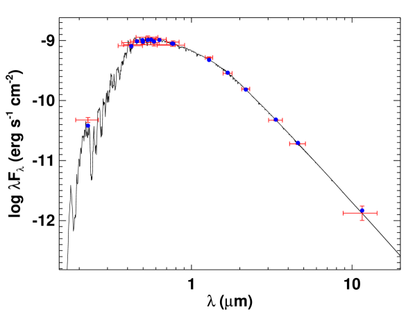
We performed a fit using phoenix stellar atmosphere models (Husser et al., 2013), with the principal free parameters being and the extinction (), which we restricted to the maximum line-of-sight value from the dust maps of Schlegel et al. (1998). The SED does not strongly constrain surface gravity () or metallicity ([Fe/H]), and hence we adopted the values from the discovery paper. The resulting fit is excellent (Figure 2) with a reduced of 1.6. The best-fit temperature is K, and the best-fit extinction is . Integrating the (unreddened) model SED gives the bolometric flux at Earth of erg s-1 cm-2. Taking the and together with the Gaia DR2 parallax, adjusted by mas to account for the systematic offset reported by Stassun & Torres (2018), we computed an updated stellar radius of R⊙.
3 Results
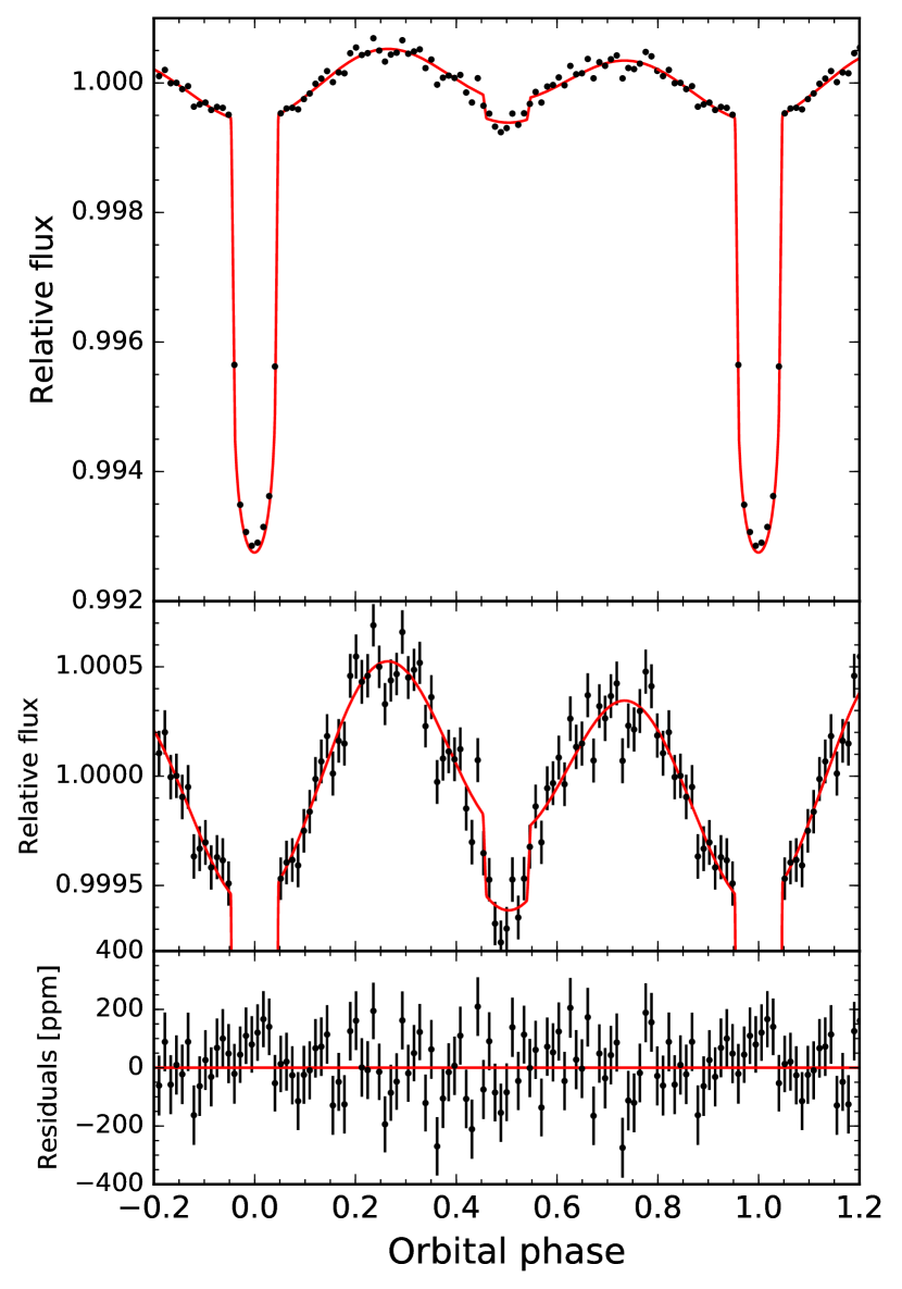
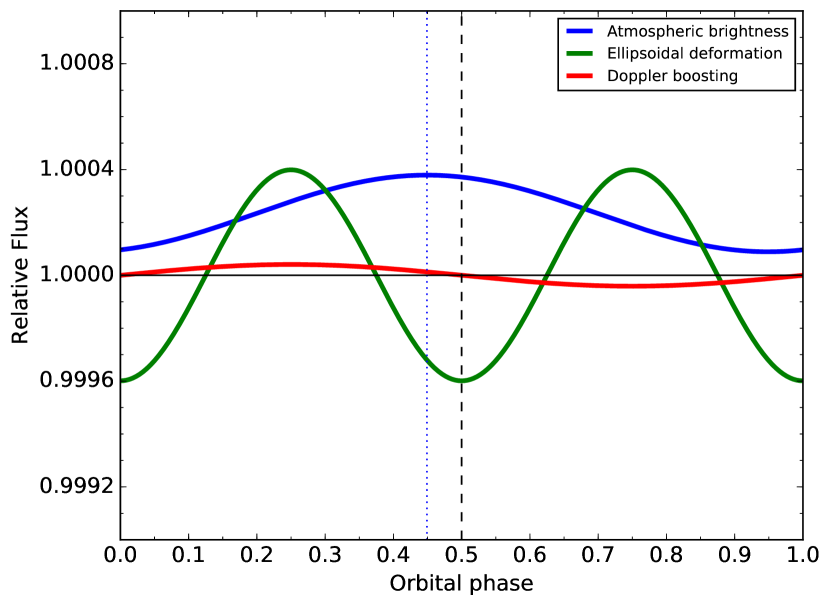
We adopted the results from polynomial detrending as the best fit values for KELT-1b’s phase curve, though all three analyses provided consistent results (Table 2). We find that KELT-1b shows a relatively large atmospheric phase curve amplitude of ppm and a mildly significant phase offset of . KELT-1b’s secondary eclipse depth is also relatively large, at ppm, while the nightside flux level is not significantly above zero. The systematics-removed, phase-folded, and binned light curve is shown in Figure 3, alongside the best-fit phase curve model. The individual components of the phase curve signal are plotted separately in Figure 4.
The Doppler boosting amplitude was constrained by Gaussian priors, and we obtained ppm. Meanwhile, the ellipsoidal distortion signal was unconstrained in our fit, and we measured an amplitude of ppm, consistent with the theoretical prediction of ppm to well within the level. This indicates that the photometric signal stemming from the tidal distortion of the host star is well-described by the physical formalism described in Equations (2)–(3).
To calculate the blackbody brightness temperatures in the TESS bandpass, we used a phoenix model spectrum Husser et al. (2013) for the host star derived using the stellar parameters from Section 2.3 and estimated the uncertainties using MCMC, following (Beatty et al., 2019). The dayside of KELT-1b has a blackbody brightness temperature of K, while the nightside has a poorly constrained brightness temperature of K.
4 Discussion
The overall system and phase curve parameters from the TESS data are generally consistent with results from the previous Spitzer phase curve observations of KELT-1b (Beatty et al., 2019). In particular, the phase curve offset in the TESS band () is similar to the measured phase offsets at 3.6 m () and 4.5 m (). This makes KELT-1b only the second sub-stellar object to have a measured offset in its TESS phase curve, after WASP-100b (Jansen & Kipping, 2020; Wong et al., 2020a), though the relatively large uncertainty on KELT-1b’s phase offset makes detailed comparisons difficult.
The measured nightside blackbody brightness temperature in the TESS band is highly uncertain. Nevertheless, it is consistent with the previously published Spitzer 3.6 m and 4.5 m nightside temperatures (Beatty et al., 2019): K and K, respectively.
One slight difference between the TESS and Spitzer system parameters is the precise value of , which is smaller by 0.0098 () in the TESS data. Since the surface gravity of KELT-1b is approximately 30 times higher than that of a typical hot Jupiter, the atmospheric scale height is very small, and the transit transmission signal is thus well below the measurement uncertainty of both observations. Therefore, in principle, the TESS and Spitzer values should match. Though the difference we measure is only suggestive at , it may be indicative of inaccuracies in the modeling of stellar limb darkening either here or in Beatty et al. (2019).
The other difference between the TESS and Spitzer phase curves is the blackbody brightness temperature of KELT-1b’s dayside in the three bandpasses. Beatty et al. (2019) measured brightness temperatures of K at 3.6 m and K at 4.5 m. While the two Spitzer dayside temperatures are mutually consistent, they are both approximately cooler than the K dayside brightness temperature we measured in the TESS bandpass. Previous ground-based observations of KELT-1b’s eclipse spectrum in the -band (Beatty et al., 2017) have indicated that KELT-1b’s dayside spectrum is not a featureless blackbody — as is common for ultra-hot Jupiters — so the larger than expected eclipse depth in the TESS bandpass prompted us to consider KELT-1b’s eclipse spectrum in more detail.
4.1 Modeling KELT-1b’s Eclipse Spectrum
In order to interpret the dayside spectrum of KELT-1b, we utilized ScCHIMERA (Piskorz et al., 2018; Arcangeli et al., 2018; Mansfield et al., 2018; Kreidberg et al., 2018; Gharib-Nezhad & Line, 2019; Zalesky et al., 2019) to produce a small grid of self-consistent 1D radiative-convective-thermochemical equilibrium models. Since previous work, the model has been upgraded to account for the latest high-temperature ExoMol (Tennyson et al., 2016) opacities (Gharib-Nezhand et al. in prep) and atomic opacities (Fe I, Fe II, Ca I, Mg I ) relevant to ultra-hot Jupiters (e.g. Lothringer & Barman, 2019). The model machinery has been previously benchmarked and validated against analytic solutions and earlier brown dwarf grid models (Saumon & Marley, 2008) in Piskorz et al. (2018) and was recently used to interpret the combined WFC3 and Spitzer spectra of the ultra-hot Jupiters WASP-18b (Arcangeli et al., 2018), HAT-P-7b (Mansfield et al., 2018), and WASP-103b (Kreidberg et al., 2018).
KELT-1b is a unique object in that while it has a dayside temperature of a typical ultra-hot Jupiter, it has the mass of a brown dwarf, and thus likely has retained a large internal heat flux, or “internal temperature”. Brown dwarf evolutionary models predict that an isolated field object with KELT-1b’s mass and age would have an internal temperature of approximately 900 K (Saumon & Marley, 2008), but the strong irradiation KELT-1b has received from its primary star has likely severely retarded KELT-1b’s cooling (Burrows et al., 2011). With this in mind, we explored a range of possible internal temperatures from 100K (similar to a cold-start like planet) to 3500K (similar to an M-dwarf). We also considered several different possible values for heat redistribution: full redistribution from the day- to nightside, dayside-only redistribution, and a minimum “hotspot” redistribution (e.g., Arcangeli et al., 2019). For simplicity we assumed solar composition, though we did change the metallicity slightly with little consequence. We utilized a 6500 K PHOENIX stellar model for the star KELT-1 (Husser et al., 2013, with 2016 upgrades).
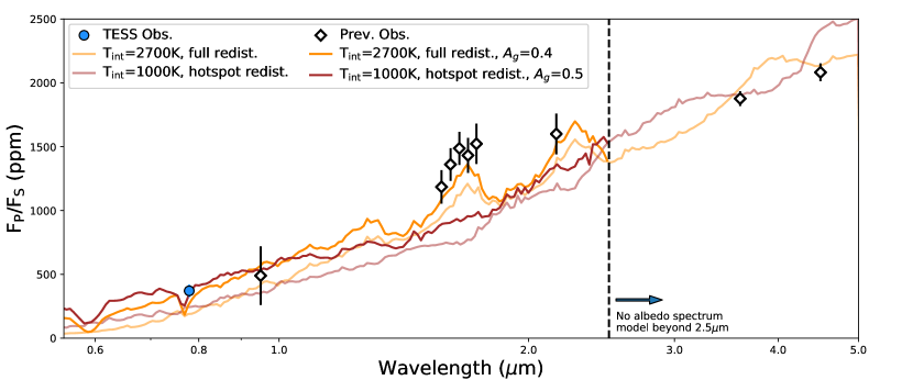
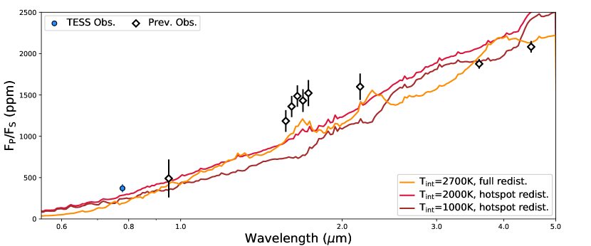
In addition to our secondary eclipse measurement in the TESS bandpass, KELT-1b’s eclipse has been also measured in (Beatty et al., 2014), -band (Beatty et al., 2017), -band (Croll et al., 2015), and from space by Spitzer at 3.6 m and 4.5 m (Beatty et al., 2019). None of the atmosphere models that we generated provided a good fit to this combined dataset. A priori one might have expected results close to the K, “hotspot” redistribution, model (Figure 5), since this matches the approximate interior luminosity KELT-1b would have if it were a field object (Saumon & Marley, 2008). However, while this model does fit the Spitzer eclipse depths, it significantly undershoots the ground-based data in the -band and -band, as well as the TESS eclipse depth.
The two best fitting models were the K with full heat redistribution model, and the K model with minimum hotspot redistribution (Figure 5) – but both were still rejected . The poor fit to these models is primarily caused by the TESS and the ground-based -band observations, which lie significantly above the model predictions. Note that both of these models would be consistent with the observed phase variation even at K, since the observed nightside brightness temperature is K.
One possible contributor to the discrepancy between the - and -band eclipse depths and our models is the presence of unmodeled ellipsoidal deformation in those measurements. Both the characteristic ellipsoidal deformation and the secondary eclipse reach their respective minima at superior conjunction, so there is a fundamental trade-off between the ellipsoidal distortion amplitude and the secondary eclipse depth. In our fits, this is manifested in a positive correlation between baseline flux of the brown dwarf and the amplitude . By not accounting for the presence of ellipsoidal deformation, the eclipse depths reported in Beatty et al. (2017) and Croll et al. (2015) may be somewhat overestimated, thereby causing the incompatibility between those - and -band measurements with the atmospheric models in Figure 5.
More extensive atmospheric modeling of KELT-1b’s dayside spectrum may provide an improved fit to the data. The ScCHIMERA models shown in Figure 5 are cloud-free 1D models that assume equilibrium chemistry, but it is likely that even for a cloud-free atmosphere the dayside of KELT-1b shows significant disequilibrium effects caused by the horizontal transport of the cooler nightside atmosphere onto the dayside.
The high surface gravity of KELT-1b – as compared to a typical hot Jupiter – may make this horizontal chemical disequilibrium more noticeable, since KELT-1b’s correspondingly high photospheric pressure inhibits most of the molecular dissociation expected on hot Jupiters’ daysides (Arcangeli et al., 2018). As an example, only 20% of the water on KELT-1b’s dayside should be dissociated, much less than the 99% water dissociation rate of a hot Jupiter like WASP-103b (Parmentier et al., 2018). There should therefore be significant amounts of water present in KELT-1b’s atmosphere, and the evolution of water absorption features (and other molecular absorption) across KELT-1b’s dayside should change significantly as the atmosphere heats up. The effect of changing spectral emission with longitude is not included in the 1D ScCHIMERA models.
4.2 A Possibly High Albedo and Morning Clouds
While the presence of unmodeled ellipsoidal deformation may resolve the discrepancy with the -band points, the higher than expected TESS band secondary eclipse requires a separate explanation. One possibility is that KELT-1b has a significant optical (and perhaps NIR) albedo. All of the models in Figure 5 consider only the thermal emission from KELT-1b’s dayside, with no accounting for a possible reflection signal. If the apparently large eclipse depth in the TESS data is due to unmodeled reflection, it would imply that KELT-1b’s dayside has a geometric albedo in the TESS bandpass of for the K model, for the K model, or for the K model.
Though HST/STIS observations of ultra-hot Jupiters have failed to detect any dayside geometric albedo in the blue-optical (Bell et al., 2017), recent analyses of TESS phase curves have begun to detect evidence for dayside significant reflection for some hot and ultra-hot Jupiters (e.g. Daylan et al., 2019; Wong et al., 2020c, a). The results from Wong et al. (2020a) are particularly interesting for the case of KELT-1b, since the marginal correlation between increasing dayside temperature and increasing geometric albedo suggested by that work would predict that KELT-1b’s albedo is to – similar to what we find under this interpretation. On the other hand, the possibly high albedo of KELT-1b disagrees with the other tentative correlation found by Wong et al. (2020a) — that the dayside geometric albedo appears to decrease with increasing planetary surface gravity. However, the interplay between surface gravity and albedo in Wong et al. (2020a) was anchored by what was then the only available high-gravity measurement: WASP-18b (Shporer et al., 2019). It is therefore possible that WASP-18b is a low-albedo outlier for some as-yet unknown reason – though this is contingent on KELT-1b having a significant dayside albedo.
One way for there to be a measurable albedo on KELT-1b’s dayside would be if there were reflective clouds present. Though the equilibrium temperature of KELT-1b’s dayside is too hot for clouds to exist in a steady-state, it is possible that clouds that form on the nightside may be blown over onto the dayside via horizontal transport in the atmosphere. For wind velocities of a few km s-1, the rough cloud lifetimes estimated by Helling et al. (2019) at these temperatures indicate that clouds could exist for a significant portion of the local morning, and potentially out to the local noon, before breaking-up on the hot dayside.
Recent analyses of Spitzer phase curves results (including that of KELT-1b) have shown that nightside clouds are likely present on all hot Jupiters (Beatty et al., 2019; Keating et al., 2019). Based on the nearly constant 1100 K nightside temperature of these planets at both 3.6 m and 4.5 m, Beatty et al. (2019) hypothesised that these were primarily silicate clouds, which agrees with simulations (e.g. Powell et al., 2018; Gao et al., 2020). Notably, high temperature silicate clouds have a spherical albedo of roughly across the TESS, -, and -bandpasses (Sudarsky et al., 2000) – similar to the geometric albedos implied above.
If we make the strong assumption that nightside silicate clouds are transported over to the morning of KELT-1b, such that , and we discount the - and band data due to un-modeled ellipsoidal deformation, then the K model becomes consistent with the observations at (Figure 6).
In principle we should be able to see an effect from any clouds present during KELT-1b’s morning in the offset of the TESS phase curve, with the significant clouds driving the phase offset to the west (i.e., negative values). Such a scenario has been detected on Kepler-7b, Kepler-12b, and Kepler-41b from the analysis of the Kepler phase curves (Shporer & Hu, 2015). We measured an eastward offset of for KELT-1b, though the uncertainty on that measurement is such that it is also consistent with an offset of zero, or even a few degrees to the west. More generally, given the opposing effects of superrotating winds on thermal emission and the westward offset from morning terminator clouds, our measured offset is likely some combination of a larger eastward thermal offset being balanced by some amount of reflective clouds in the western hemisphere.
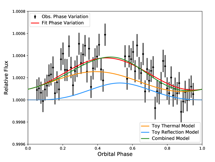
One aspect regarding a possible high albedo for KELT-1b is that in our fitting process we assumed that the phase variation from KELT-1b is well-modeled by a single sinusoid (Section 2.1), and not by a two-component thermal emission and reflected light model (e.g., Esteves et al., 2015). However, given the size of the data uncertainties relative to the measured phase amplitude (Figures 3 and 7), we considered a more detailed fit to the data to be unwarranted. That being said, as shown in Figure 7 it is possible to replicate the observed phase variation using a toy model of combined thermal emission and Lambertian reflected light. In this particular case, we assumed that the albedo of the reflected light component is , which is consistent with our suggested albedo of . Note, though, that the combined thermal plus reflected light model shown in Figure 7 is primarily for illustrative purposes — to demonstrate that the observed sinusoidal phase variation is also consistent with KELT-1b having a high dayside albedo. A full detailed two-component model fit would need to account for the non-sinusoidal thermal emission seen in the Spitzer phase curve of hot Jupiters (Beatty et al., 2019) as well as the complex non-Lambertian reflection signal caused by non-uniform dayside clouds.
5 Summary and Conclusions
We have presented our analysis of the TESS full-orbit phase curve of the transiting brown dwarf KELT-1b. We fit the data using a combined model for the secondary eclipse, atmospheric brightness modulation, and the ellipsoidal deformation and Doppler boosting of the primary star. We detrended the TESS data using three different approaches: polynomial detrending, a Gaussian-Process regression, and a Fourier decomposition of the out-of-transit light curve. The results from all three analyses are consistent with each other, and we adopted the values from the polynomial detrending fit as our primary set of results.
We found that KELT-1b shows significant phase variation in the TESS bandpass, with a relatively large phase amplitude of ppm and a secondary eclipse depth of ppm. We also measured a marginal phase offset of , though given the relatively large uncertainty on the offset measurement this result is also consistent with zero.
Our measurement of the TESS eclipse and the other measurements of KELT-1b’s secondary eclipse at other wavelengths give us a interesting view of the brown dwarf’s dayside emission (Figure 5). We modeled this emission using a grid of results from the ScCHIMERA atmosphere models, with KELT-1b’s interior temperature and the amount of heat redistribution as the two primary variables affecting the model results. We found three possible fits: one at K with full heat redistribution, one at K with minimum hotspot redistribution, and a model at K also with hotspot redistribution. However, all these models are inconsistent with the combined dayside spectrum at .
Since the ScCHIMERA models assume 1D, cloud-free, equilibrium chemistry in their calculations, it is possible that the poor fit to the data is caused by these assumptions. Meanwhile, for the higher than expected -band eclipse measurements from Beatty et al. (2017), unmodeled ellipsoidal distortion may explain the discrepant depth measurements relative to our models. In general, KELT-1b may show stronger 2D disequilibrium effects than a typical hot Jupiter. Horizontal transport of cooler nightside atmosphere onto the dayside may introduce a significant source of molecular absorption – particularly since the high surface gravity of KELT-1b prevents almost all of the dayside molecular dissociation expected on a typical hot Jupiter. In particular, there should be significant water present on KELT-1b’s dayside (Parmentier et al., 2018).
Given the relatively large eclipse depth we measure in the TESS bandpass, the dayside of KELT-1b may have a significant geometric albedo of . We hypothesize that this could be caused by the presence of high temperature silicate clouds (Gao et al., 2020) that form on KELT-1b’s nightside and extend significantly onto the morning half of KELT-1b’s dayside before breaking up (e.g. Helling et al., 2019). If we grant that the - and -band eclipse depths are systematically higher due to un-modeled effects from ellipsoidal deformation, then under this hypothesis the K atmosphere model, with a reflection component, is likely the best fit to the data (Figure 6). This interior temperature agrees with KELT-1b’s expected interior temperature given its mass and age (Saumon & Marley, 2008), and is consistent with the nightside temperatures measured here and in the Spitzer data (Beatty et al., 2019).
A high geometric albedo for KELT-1b’s dayside would be consistent with the tentative trend found by Wong et al. (2020a) that hot Jupiters with higher dayside temperatures show higher geometric albedos. Though the steady-state temperatures of these planets’ (and KELT-1b’s) daysides are too hot for clouds (e.g. Parmentier et al., 2016; Helling et al., 2019), recent ensemble analyses of Spitzer phase curves of hot Jupiters (Beatty et al., 2019; Keating et al., 2019) concluded that these planets universally possess nightside clouds. It is possible that clouds forming on the planetary nightsides may be blown over onto the daysides via horizontal transport (e.g. Helling et al., 2019). As these clouds break-up on the hot dayside they could provide a significant reflection signal (Marley et al., 1999; Sudarsky et al., 2000).
If KELT-1b does indeed have a significant dayside albedo caused by partial silicate cloud cover, this would be a strong demonstration of the importance of including horizontal transport and its effect on planetary cloud coverage in 3D atmospheric simulations, as well as the inclusion of cloud effects in 1D modeling of hot Jupiter eclipse spectra.
References
- Angerhausen et al. (2015) Angerhausen, D., DeLarme, E., & Morse, J. A. 2015, PASP, 127, 1113
- Arcangeli et al. (2018) Arcangeli, J., Désert, J.-M., Line, M. R., et al. 2018, ApJ, 855, L30
- Arcangeli et al. (2019) Arcangeli, J., Désert, J.-M., Parmentier, V., et al. 2019, A&A, 625, A136
- Astropy Collaboration et al. (2013) Astropy Collaboration, Robitaille, T. P., Tollerud, E. J., et al. 2013, A&A, 558, A33
- Astropy Collaboration et al. (2018) Astropy Collaboration, Price-Whelan, A. M., Sipőcz, B. M., et al. 2018, AJ, 156, 123
- Beatty et al. (2017) Beatty, T. G., Madhusudhan, N., Pogge, R., et al. 2017, AJ, 154, 242
- Beatty et al. (2019) Beatty, T. G., Marley, M. S., Gaudi, B. S., et al. 2019, AJ, 158, 166
- Beatty et al. (2014) Beatty, T. G., Collins, K. A., Fortney, J., et al. 2014, ApJ, 783, 112
- Bell et al. (2017) Bell, T. J., Nikolov, N., Cowan, N. B., et al. 2017, ApJ, 847, L2
- Benneke et al. (2019) Benneke, B., Knutson, H. A., Lothringer, J., et al. 2019, Nature Astronomy, 3, 813
- Bourrier et al. (2020) Bourrier, V., Kitzmann, D., Kuntzer, T., et al. 2020, A&A, 637, A36
- Burrows et al. (2011) Burrows, A., Heng, K., & Nampaisarn, T. 2011, ApJ, 736, 47
- Claret (2017) Claret, A. 2017, A&A, 600, A30
- Claret (2018) —. 2018, A&A, 618, A20
- Croll et al. (2015) Croll, B., Albert, L., Jayawardhana, R., et al. 2015, ApJ, 802, 28
- Daylan et al. (2019) Daylan, T., Günther, M. N., Mikal-Evans, T., et al. 2019, apj, in revision, arXiv:1909.03000
- Demory et al. (2013) Demory, B.-O., de Wit, J., Lewis, N., et al. 2013, ApJ, 776, L25
- Esteves et al. (2015) Esteves, L. J., De Mooij, E. J. W., & Jayawardhana, R. 2015, ApJ, 804, 150
- Evans et al. (2013) Evans, T. M., Pont, F., Sing, D. K., et al. 2013, ApJ, 772, L16
- Foreman-Mackey et al. (2017) Foreman-Mackey, D., Agol, E., Ambikasaran, S., & Angus, R. 2017, AJ, 154, 220
- Foreman-Mackey et al. (2013) Foreman-Mackey, D., Hogg, D. W., Lang, D., & Goodman, J. 2013, PASP, 125, 306
- Gao et al. (2020) Gao, P., Thorngren, D. P., Lee, G. K. H., et al. 2020, Nature Astronomy, doi: 10.1038/s41550-020-1114-3
- Gharib-Nezhad & Line (2019) Gharib-Nezhad, E., & Line, M. R. 2019, ApJ, 872, 27
- Gibson et al. (2012) Gibson, N. P., Aigrain, S., Roberts, S., et al. 2012, MNRAS, 419, 2683
- Han et al. (2014) Han, E., Wang, S. X., Wright, J. T., et al. 2014, PASP, 126, 827
- Helling et al. (2019) Helling, C., Iro, N., Corrales, L., et al. 2019, A&A, 631, A79
- Husser et al. (2013) Husser, T. O., Wende-von Berg, S., Dreizler, S., et al. 2013, A&A, 553, A6
- Jansen & Kipping (2020) Jansen, T., & Kipping, D. 2020, MNRAS, 494, 4077
- Jenkins et al. (2016) Jenkins, J. M., Twicken, J. D., McCauliff, S., et al. 2016, Society of Photo-Optical Instrumentation Engineers (SPIE) Conference Series, Vol. 9913, The TESS science processing operations center, 99133E
- Keating et al. (2019) Keating, D., Cowan, N. B., & Dang, L. 2019, Nature Astronomy, 3, 1092
- Kreidberg (2015) Kreidberg, L. 2015, PASP, 127, 1161
- Kreidberg et al. (2018) Kreidberg, L., Line, M. R., Parmentier, V., et al. 2018, AJ, 156, 17
- Loeb & Gaudi (2003) Loeb, A., & Gaudi, B. S. 2003, ApJ, 588, L117
- Lothringer & Barman (2019) Lothringer, J. D., & Barman, T. 2019, ApJ, 876, 69
- Mandel & Agol (2002) Mandel, K., & Agol, E. 2002, ApJ, 580, L171
- Mansfield et al. (2018) Mansfield, M., Bean, J. L., Line, M. R., et al. 2018, AJ, 156, 10
- Marley et al. (1999) Marley, M. S., Gelino, C., Stephens, D., Lunine, J. I., & Freedman, R. 1999, ApJ, 513, 879
- Mayorga et al. (2019) Mayorga, L. C., Batalha, N. E., Lewis, N. K., & Marley, M. S. 2019, AJ, 158, 66
- Mazeh & Faigler (2010) Mazeh, T., & Faigler, S. 2010, A&A, 521, L59
- Ochsenbein et al. (2000) Ochsenbein, F., Bauer, P., & Marcout, J. 2000, A&AS, 143, 23
- Oreshenko et al. (2016) Oreshenko, M., Heng, K., & Demory, B.-O. 2016, MNRAS, 457, 3420
- Parmentier et al. (2016) Parmentier, V., Fortney, J. J., Showman, A. P., Morley, C., & Marley, M. S. 2016, ApJ, 828, 22
- Parmentier et al. (2018) Parmentier, V., Line, M. R., Bean, J. L., et al. 2018, A&A, 617, A110
- Piskorz et al. (2018) Piskorz, D., Buzard, C., Line, M. R., et al. 2018, AJ, 156, 133
- Powell et al. (2018) Powell, D., Zhang, X., Gao, P., & Parmentier, V. 2018, ApJ, 860, 18
- Saumon & Marley (2008) Saumon, D., & Marley, M. S. 2008, ApJ, 689, 1327
- Schlegel et al. (1998) Schlegel, D. J., Finkbeiner, D. P., & Davis, M. 1998, ApJ, 500, 525
- Schneider et al. (2011) Schneider, J., Dedieu, C., Le Sidaner, P., Savalle, R., & Zolotukhin, I. 2011, A&A, 532, A79
- Shporer (2017) Shporer, A. 2017, PASP, 129, 072001
- Shporer & Hu (2015) Shporer, A., & Hu, R. 2015, AJ, 150, 112
- Shporer et al. (2019) Shporer, A., Wong, I., Huang, C. X., et al. 2019, AJ, 157, 178
- Siverd et al. (2012) Siverd, R. J., Beatty, T. G., Pepper, J., et al. 2012, ApJ, 761, 123
- Smith et al. (2012) Smith, J. C., Stumpe, M. C., Van Cleve, J. E., et al. 2012, PASP, 124, 1000
- Stassun et al. (2017) Stassun, K. G., Collins, K. A., & Gaudi, B. S. 2017, AJ, 153, 136
- Stassun et al. (2018) Stassun, K. G., Corsaro, E., Pepper, J. A., & Gaudi, B. S. 2018, AJ, 155, 22
- Stassun & Torres (2016) Stassun, K. G., & Torres, G. 2016, AJ, 152, 180
- Stassun & Torres (2018) Stassun, K. G., & Torres, G. 2018, ApJ, 862, 61
- Stumpe et al. (2014) Stumpe, M. C., Smith, J. C., Catanzarite, J. H., et al. 2014, PASP, 126, 100
- Sudarsky et al. (2000) Sudarsky, D., Burrows, A., & Pinto, P. 2000, ApJ, 538, 885
- Tennyson et al. (2016) Tennyson, J., Yurchenko, S. N., Al-Refaie, A. F., et al. 2016, Journal of Molecular Spectroscopy, 327, 73
- von Essen et al. (2020) von Essen, C., Mallonn, M., Borre, C. C., et al. 2020, A&A, 639, A34
- Wenger et al. (2000) Wenger, M., Ochsenbein, F., Egret, D., et al. 2000, A&AS, 143, 9
- Wong et al. (2020a) Wong, I., Shporer, A., Daylan, T., et al. 2020a, AJ, 160, 155
- Wong et al. (2020b) Wong, I., Shporer, A., Kitzmann, D., et al. 2020b, AJ, 160, 88
- Wong et al. (2020c) Wong, I., Benneke, B., Shporer, A., et al. 2020c, AJ, 159, 104
- Wong et al. (2020d) Wong, I., Shporer, A., Becker, J. C., et al. 2020d, AJ, 159, 29
- Zalesky et al. (2019) Zalesky, J. A., Line, M. R., Schneider, A. C., & Patience, J. 2019, ApJ, 877, 24
| Parameter | Description and Units | Gaussian Process | Out-of-Transit | |
|---|---|---|---|---|
| System ParametersaaConstrained by Gaussian priors (see Table 1 and Section 2.1).: | ||||
| Transit time () | — | |||
| Orbital period (days) | — | |||
| Cosine of inclination | — | |||
| Radius ratio | — | |||
| Semi-major axis in stellar radii | — | |||
| bbIn the fit using polynomial detrending (Section 2.2.1), the ellipsoidal deformation amplitude is a free parameter, from which the system mass ratio is subsequently derived; vice versa for the case of GP regression (Section 2.2.2). | Mass ratio | — | — | |
| Phase Curve Parameters: | ||||
| Phase baseline (ppm) | — | |||
| Phase amplitude (ppm) | 195 | |||
| Phase offset (deg.) | 18 | |||
| bbIn the fit using polynomial detrending (Section 2.2.1), the ellipsoidal deformation amplitude is a free parameter, from which the system mass ratio is subsequently derived; vice versa for the case of GP regression (Section 2.2.2). | Ellipsoidal def. amplitude (ppm) | 415 | ||
| aaConstrained by Gaussian priors (see Table 1 and Section 2.1). | Dopp. beaming amplitude (ppm) | 41 | ||
| Derived Parameters: | ||||
| Secondary eclipse depth (ppm) | — | |||
| Nightside flux (ppm) | — | |||
| Phase maximum (ppm) | — | |||
| Phase minimum (ppm) | — | |||
| Secondary eclipse time () | — | |||
| Inclination (deg.) | — | |||
| Impact parameter | — | |||
| SED-fit and Derived Parameters: | ||||
| Stellar radius () | — | — | ||
| Brown dwarf radius () | — | — | ||