Cyclic space-filling curves and their clustering property

Abstract

In this paper we introduce an algorithm of construction of cyclic space-filling curves. One particular construction provides a family of space-filling curves in all dimensions (H-curves). They are compared here with the Hilbert curve in the sense of clustering properties, and it turns out that the constructed curve is very close and sometimes a bit better than the Hilbert curve. At the same time, its construction is more simple and evaluation is significantly faster.

Introduction

A space-filling curve in dimension $d$ is a map from $[0,1]$ into $\mathbb{R}^{d}$ such that the image contains an open non-empty set or, equivalently, some cube $[a_{1},b_{1}]\times\ldots\times[a_{d},b_{d}]$ for $a_{i}<b_{i}$, $i=1,\ldots,d$. There are lots of space filling curve constructions, many of them can be found in [1].

Fractal space-filling curves are self-similar curves, i. e. they exhibit similar patterns at increasingly small scales. This similarity is called unfolding symmetry. If the symmetry is a composition of scale and an isometry, the curve is called affine self-similar.

Affine self-similar curves play an important role in practice, because they can be easily constructed and provide a way to construct locality-preserving mapping from multidimensional data into one-dimensional space. For instance, the applications include

• geo-information systems (GIS, see [2]),

• database indices (map multidimensional data to one-dimensional disk address space, see [3]),

• image compression (clustering of pixels by three-dimensional color, see [4]),

• parallel processing (see [5]),

• bandwidth reduction of digitally sampled signals (see [6]).

There are many sophisticated curve constructions in the literature. The simplest curve construction which is also called Z-curve was proposed in [7]. Its improvement by usage of Grey coding was proposed in [8]. Another method based on the Hilbert curve [9] was proposed in [10].

The first space-filling curve was discovered by G. Peano in 1890. This curve is continuous in terms of Jordans’s precise notion of continuity (1887). In 1891 D. Hilbert discovered a general geometric construction procedure for a class of space-filling curves [9]. It has been shown that the Hilbert curve is a continuous, surjective and nowhere differentiable mapping [11].

We follow the procedure mentioned above with some modification making all the constructed curves cyclic thus leading to a class of continuous space-filling curves $S^{1}\to[0,1]^{d}$. Constructions in [9] are based on ordering, i. e. one subdivides a cube into a grid of half-size cells being recursively divided up to $2^{nd}$ unit cells (assuming that the initial cube has size length $2^{n}$), where $n$ the depth of subdivision. Then an order of half-size cells is chosen and an order of unit cells is recursively defined, thus giving the ordering of all unit cells. We apply a different approach including construction of oriented cycles and combining them to a single oriented cycle on each step of the construction. Resulting class of curves differs from the order-based space-filling curves. Its advantage is the simpler algorithmic description of continuous curves. In the case of order-based construction we must apply some reflections (or any of $2^{d}\cdot d!$ symmetries) to sub-cells. In the case of cycle-based construction we can avoid usage of all sub-cell symmetries and only apply rotations and/or reversals of cycles obtaining the curve which we call H-curve. In terms of evaluation this can be expressed as an linear operation modulo length of the cycle of the form $x\mapsto\pm x+c$.

Not only fractal curves are used in practice. For example, the onion curve [12] and spectral curve [13] can give better results than the Hilbert curve, but have a fixed space granularity. Fractal curves have the advantage that one can select granularity and evaluate indexes with different precision for different points. For example, if we need only to compare the ordering of a pair of points, we need only to evaluate indexes until the first difference occurred.

Let us describe carefully the notion of locality-preserving mappings. Roughly speaking, we want to construct such a mapping $\omega$ that the closer the images $\omega(x),\omega(y)\in\mathbb{R}^{d}$ of two points are, the closer the points $x,y\in\mathbb{R}$ are and vice versa (like it is described in [1]). In other words, one condition is that the mapping $\omega$ is open and other is that $\omega$ is continuous. Unfortunately, there are no curves satisfying both these conditions.

If a curve is a one-to-one correspondence (we need it to be injection, because we consider only surjective mappings by the definition of space-filling curves), then it is a homeomorphism (open continuous bijection). But the interval $[0,1]$ and a cube $[0,1]^{d}$ for $d>1$ are not homeomorphic, because $[0,1]$ without any point except $0$ and $1$ is not connected and $[0,1]^{d}$ without any point is connected. Number (more precisely, cardinality) of points $x\in X$ for a topological space $X$ such that $X\setminus\{x\}$ is disconnected is a topological invariant and preserves under homeomorphisms. The subset of such points in $[0,1]^{d}$ is empty for $d>1$ and is $(0,1)$ for $d=1$, so we get a contradiction.

We will see below that the curves we consider are not one-to-one correspondences. Nevertheless, there are no open continuous mappings from $[0,1]$ to $[0,1]^{d}$ for $d>1$.

Now suppose that a curve $\omega\colon[0,1]\to[0,1]^{d}$ is continuous, open and is not injective. By an equivalent definition of continuous map, it is a map such that the preimage of a closed subset is closed. Therefore, for any point $v\in[0,1]^{d}$ as a closed subset its preimage $\omega^{-1}(v)\subseteq[0,1]$ is a closed subset of the compact $[0,1]$, i. e. is compact and therefore includes its minimum, so $\omega(\min(\omega^{-1}(v)))=v$. Define $S=\{\min(\omega^{-1}(v))\,\mid\,v\in[0,1]^{d}\}\subseteq[0,1]$. From non-injectivity it follows that $S\neq[0,1]$. Obviously, $0\in S$. If $S=[0,1)$, then we get a contradiction in the same way as before. Otherwise $p\in(0,1)\setminus S$ exists, i. e. the set $S$ is not connected. But the mapping $\omega\colon S\to[0,1]^{d}$ is open, continuous and bijective by construction. Therefore, $S$ and $[0,1]^{d}$ are homeomorhic. At the same time, $[0,1]^{d}$ is connected and $S$ is not, so we again get a contradiction.

This simple topological reasoning shows that we need to weaken the conditions on locality preserving mappings. We can obtain continuity, but we need some other way to compare which of curves “better preserves locality”. Here we follow a well-known idea from [3] (see §3) to compare numbers of “connected components of preimages of connected figures” asymptotically for curve construction iterations. In the same way, we perform a numerical simulation experiment and obtain results (see §3.2).

Another interesting property of such maps (like Hilbert curve) is that they are measure-preserving, i. e. if $S\subseteq[0,1]$ has one-dimensional Lebesque measure $z$, then its image $\{\omega(s)\,\mid\,s\in S\}$ has $d$-dimensional Lebesque measure $z$. We omit the proof of this property as a simple analysis exercise.

The idea of continuity is a useful heuristic to construct curves with better locality preserving properties. The main results of this paper are

• to introduce the idea of cyclicity (see §1),

• to construct an explicit cyclic curve for any dimension (see §2),

• to conduct an experiment providing an empirical evidence that the constructed curve is slightly better (or not worse) than the Hilbert curve,

• to show that the construction of the these curves is simpler than the construction of most widely used Hilbert curve.

• to show by profiling that H-curve can be evaluated essentially faster than the Hilbert curve.

So, for a number of applications this new construction method may be preferable to the Hilbert curve.

1 Constructions of curves

The generic construction process of fractal space-filling curve is usually iterative. We need to map an interval size of $1$ to a square size of $1$ (or a cube of dimension $d$). Let us illustrate this for dimension $d=2$. On the first step, we divide the square into a grid of $2\times 2$ square cells, while the interval size of $1$ is subdivided into four equal sub-intervals where each sub-interval matches a cell. We say that the curve traverses the cells in the order given by the order of intervals. Then we apply the procedure recursively to each sub-interval-cell pair, so that within each cell, the curve makes a similar traversal up to symmetries of the whole cell. The symmetries are needed to make each cell’s first sub-cell touching the previous cell’s last subcell. This condition after the going to the limit gives us continuity. Let us present a more detailed algorithm.

Usually the construction of fractal space-filling curves consists of the following steps:

• divide a cube of dimension $d$ into the grid of $2^{d}$ half-size cells and match them to $2^{d}$ equal sub-intervals of interval;

• perform the iteration steps: given a matching between $2^{dn}$ cells in the cube and $2^{nd}$ sub-intervals in the interval,

  • subdivide each cell into the grid of $2^{nd}$ sub-cells (and maybe apply some symmetry of cell) and match them to sub-intervals of the corresponding sub-interval,

  • join this to the matching between grid of $2^{d(n+1)}$ cells of the cube and $2^{d(n+1)}$ sub-intervals of the interval.

Here we introduce another algorithm of curve design based on cyclicity. We assume that all the curves are cyclic. Then on the iteration step we perform some local mutation gathering $2^{d}$ cycles into one cycle. The local mutation here means the following:

• in each cell we take some subcell and the next one in the cycle,

• for these cells we say that the corresponding next subcells are next to the chosen in the next cell,

• so, for the next subcell w. r. t. the chosen one is the subcell chosen in the previous cell.

In terms of graphs, we chain $2^{d}$ edges into a cycle by $2^{d}$ edges and then remove the initial edges. If we take pairs of sub-cells in such a way that new edges connected by cycle are touching, then we obtain a continuous surjective map going to the limit:

$$S^{1}\to[0,1]^{d}.$$

See examples of local mutations in §2.

Usually one needs to perform some transformations during construction process to obtain continuity. Sometimes it is not necessary as in case of Z-curve. It is the simplest curve used, but it is not having continuity, so it has bad locality preserving properties and is not widely used. Usually, any continuous curve gives better results, but it that case the construction procedure needs carefully chosen reflections and/or rotations.

In the proposed construction of cyclic curves on the step of local mutation in terms of traversal we may need to change the traversal direction and initial point. Note that the cycle lengths are always degrees of $2$. So, the change of initial point is simply the addition of cell index to a number of new initial point modulo a degree of $2$ (addition of $d$-bit numbers), and change of direction with change of initial point to the previous one (before reversal) is simply a bitwise complement of d-bit number.

Of course, one may need to use some symmetries depending on the particular curve construction algorithm. In the section 2 we will see that a cyclic continuous curve can be constructed for any dimension without usage of any symmetries. An addition with maybe one bitwise complement is computationally cheaper than the evaluation and application of symmetry.

2 H-curve

2.1 Construction

This section is devoted to the construction of cyclic fractal space-filling curve for any $d>1$ without using symmetries. For any dimension $d$, we will traverse half-sized cells in the initial cube in the same way.

Taking a $d$-bit number k as an index in traversal (counting from $0$), we obtain the corresponding cell coordinate bits as consecutive bits of the number

$$g_{d}(k):=k\oplus\lfloor(k\mod 2^{d})/2\rfloor\mod 2^{d}$$

(the symbol $\oplus$ means bitwise sum, or, xor). This function permutes the set $\{0,\ldots,2^{d}-1\}$. Therefore, the function $g_{d}^{-1}$ is well-defined on the set $\{0,\ldots,2^{d}-1\}$.

As we claimed, in the cells we do not apply any reflections or rotations to the cells and sub-cells. For the curve construction we need only the local mutations. For explicit computation of correspondence between indexes and cells we need to calculate the index shifts and find all direction reversals.

2.2 Local mutation

For convenience let us assume that grid cells are unit cubes, and the initial big cube has side length $2^{n}$.

Actually, for any dimension $d>1$ we will apply the same local mutation. This mutation will always act on the central $4\times 2\times\ldots\times 2$-parallelepiped.

Lemma 2.1.

Given $d>1$, for any $n\geqslant 2$ the restriction of the graph composed of $2^{d}$ half-size cycles in the cube with side length $2^{n}$ onto the central $4\times 2\times\ldots\times 2$-parallelepiped form the same graph, namely, if we denote its vertices with $\{0,1,2,3\}\times\{0,1\}^{d-1}$, then the edge set would be

$$(\{0\}\times p,\{1\}\times p)\text{ and }(\{2\}\times p,\{3\}\times p)\text{ for all }p\in\{0,1\}^{d-1}.$$

Proof.

Assume that we have the grid of integral points in the cube $[0,2^{n+1}-1]^{d}$, and we initially have the cyclic traversals of cubes of side $2$. They form a grid of $2^{n}$ cells. Then we consequently apply mutations gathering cycles into cycles traversing cells of sizes $4,8,\ldots,2^{n+1}$. Each time we consider the central $4\times 2\times\ldots\times 2$-parallelepiped in some cell of size $4,8,\ldots,2^{n+1}$, then each of these parallelepipeds has even minimal first coordinate and odd minimal other coordinates. This implies that the restrictions of initial $2^{nd}$ cycles on them are same and coincide with the written above graph. At the same time, these parallelepipeds have pairwise non-intersecting sets of vertices. Therefore, mutations of previous steps of construction do not affect the final step. ∎

On Fig. 1, 2, 3 we see examples of mutations. On these figures we color some black edges red. Then we draw a number of green edges such that together the green and red edges form cycles. After the mutation we remove red edges and color green edges black. Note that if in the red-green cycle we contract all the red edges, then we obtain exactly the graph corresponding to the traversal of the cube of size $2$ and the same dimension. Obviously, we will see the same behavior in any dimension.

Example 2.2.

Consider the case of $d=2$ and $n=3$ (side length $8$).

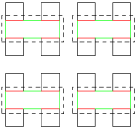
Figure 1: Join of cycles in squares of side $2$ into cycles in squares of side $4$.

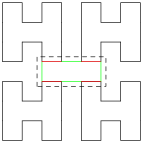
Figure 2: Join of cycles in squares of side $4$ into cycles in squares of side $8$.

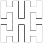
Figure 3: H-curve for $d=2$, $n=3$.

On fig. 1 we join cycles of side length $2$, after on fig. 2 we join cycles of side $4$, and on fig.  3 we see the result.

Definition 2.3.

We call the constructed above family of curves H-curves for all $d>1,n$. Also, we will call H-curves the limit curves for all $d>1$.

We name them this way for the form of the second iteration of plane curve. Next iterations also looks like the letter ‘H’, but more tangled and shaggy. For $d\geqslant 3$ we can consider these curves as high-dimensional “generalizations” of letter ‘H’.

Example 2.4.

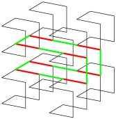
Figure 4: Example of H-curve for $d=3,n=2$ and the central mutation.

On fig. 4 we see the example of H-curve for $d=3,n=2$ (side length $4$) and how looks the mutation in three-dimensional case. In the higher dimensions it looks the same, but less illustrative.

Theorem 2.5.

For any $n\in\mathbb{N}$ and any $d>1$ the H-curve cyclically traverses all the unit cells. Each move to the next cell is a move to an adjacent cell.

For any $k<n$, for one cycle the curve one time enters and one time leaves any of cells of grid of $2^{dk}$-side cells, and the traversal of these cells is H-curve for the pair $(d,k)$.

For $n\to\infty$ we can choose infinitely decreasing sequence of cells such that each one contains all the following, and we obtain the sequence that converges to the continuous map $h\colon S^{1}\to[0,1]^{d}$.

Proof.

The first part of statement is obvious by the construction of curve and by choice of the mutation.

The second part is obvious for $k=n-1$ by the iteration of construction and for any $k$ by induction from $n-1$ down to $1$.

For the third part we need to take unit cells in such a way that

• for increasing $n$ the matching between smaller cells and intervals is a subdivision of matching between larger cells and intervals;

• end points of $[0,1]$ are mapped to the same point.

Actually, it is enough to take the first cell of initial subdivision of each next time to take the first sub-cell, where the cycle enters the cell. The condition that $0$ and $1$ are mapped into the same point is obvious. Continuity is standard and follows from the same reasons as for Hilbert and other curves. ∎

We will compare below properties of H-curve, Hilbert curve and Z-curve.

Remark 2.6.

Actually, for dimension $2$ there is only one construction method of the Hilbert. As it was noticed in [1], for higher dimensions there are many ways to generalize the construction of the curve to any dimension such that its restriction to $d=2$ gives the usual plane Hilbert curve. In [1] there are $5$ ways to do this. The commonly used version seems to be called Butz-Hilbert curve in [1]. For higher dimensions is seems that different variations of Hilbert curve would give very close results. At the same time, their constructions have the same complexity (computational and mathematical). So, we will compare H-curve with the commonly used Butz-Hilbert curve.

Remark 2.7.

One of curves constructed in [1] is called there inside-out curve. For $n=2$, it returns to the cell adjacent to the initial point, but for bigger $n$ it loses continuity. In this sense H-curve can be called an inside-out-repeat curve as a curve moving from the center to the perimeter in one octant, back to the center, out into another octant and so on cyclically.

On fig. 5 we see Z-curve, Hilbert curve and H-curve on plane. On fig. 6 we see Z-curve, Butz–Hilbert curve and H-curve in the same axes.

Figure 5: Z-curve, Hilbert curve, H-curve for $d=2,n=4$

Figure 6: Z-curve, Butz–Hilbert curve, H-curve for $d=3,n=2$

2.3 Index shifts and direction reversals

Our next goal is to describe the correspondence between a unit cell with coordinates $\overline{a}=(a_{0},\ldots,a_{d})$ in $d$-dimensional cube with side length $2^{n}$ and its index $r$ in the traversal along H-curve. Say, we encode the point $\overline{a}$ by the index $r$ and decode the index $r$ to the point $\overline{a}$. So, we want to describe two mutually inverse functions

We will construct the functions recursively. To make the construction easier, let us introduce some notation.

Let us write bits of $d$-bit numbers $a_{i}$ into the matrix $n\times d$ as rows. Denote $n$-bit numbers in the rows of transposed matrix by $\alpha^{0},\ldots,\alpha^{d}$. These coordinates are also known as coordinates in Z-order. It is easy to pass from $(a_{i})$ to $(\alpha^{j})$ and back, but $\alpha^{j}$ are more convenient for algorithm design. So, we will describe functions

Geometrical sense of $\alpha$-coordinates corresponds to the iterative construction of curve. Each cell can be coded by $d$ bits of coordinates. These $d$ bits form the number $\alpha^{j}$ for $j$-th iteration. When subdividing the cube into the grid of $2^{d}$ cells, we choose one of them which has coordinates $(\alpha^{0},\ldots,\alpha^{d-1})$.

Lemma 2.8.

The central $4\times 2\times\ldots\times 2$-parallelepiped in $d$-dimensional cube with side $2^{n}$ consists of the set of points

$$c_{\alpha}=(\alpha,\overline{\alpha},\ldots,\overline{\alpha})\text{ and }c_{\alpha}^{\prime}=(\alpha,\overline{\alpha},\ldots,\overline{\alpha}\oplus 1)$$

for all $\alpha\in\mathbb{F}_{2}^{n}$.

Proof.

Denote the central cube of size $2$ by $C$ and the central $4\times 2\times\ldots\times 2$-parallelepiped by $P$. Each half-size cube $\alpha$ has a unique unit cell in $C$. Denote it by $c_{\alpha}$. Each half-size cube $\alpha$ has two unit cells in $P$, $c_{\alpha}$ is on of them. Denote the other one by $c_{\alpha}^{\prime}$. The index $\alpha$ for both $c_{\alpha}$ and $c_{\alpha}^{\prime}$ corresponds to the first coordinate of f unit cell in $\alpha$-coordinates. Our goal is to find remaining $\alpha$-coordinates of these points.

Bits of $\alpha$ geometrically mean the choice of half-size cube in the first subdivision operation. To get the cell $c_{\alpha}\in C$, we should take opposite coordinate choices for each coordinate on each next iteration. This exactly implies that all the next $\alpha$-coordinates equal $\overline{\alpha}$.

To take $c_{\alpha}^{\prime}$, we should take the same sub-cells until the last subdivision. At the last iteration we should change the first coordinate to get the adjacent cell along the first coordinate. This exactly means that $c_{\alpha}^{\prime}$ has all next coorinates equal $\overline{\alpha}$ until the last one which equals $\overline{\alpha}\oplus 1$. ∎

Corollary 2.9.

The traversal of H-curve enters the half-size sub-cell $\alpha$ at one of unit cells $c_{\alpha}$ and $c_{\alpha}^{\prime}$ and leaves at other one.

We have fixed the traversal of the central $4\times 2\times\ldots\times 2$-parallelepiped. Therefore, if we know the order of traversal of the pair $(c_{\alpha},c_{\alpha}^{\prime})$, then we know if we need to reverse the traversal of half-size sub-cell $\alpha$. (As it was noted above, they are neighbors in the sub-cell traversal).

Now we want to determine when the direction of half-size sub-cube traversal is either the same or opposite to the direction of traversal of these sub-cubes. Suppose the direction is the same. Then before the mutation we pass from one cell of $\{c_{\alpha},c_{\alpha}^{\prime}\}$ to another one, so, traversing the remaining part of the cycle traversing the sub-cube, we pass them in the opposite order, because the first one becomes the leaving unit cell, and other one becomes the entering unit cell for sub-cube. Vice versa, if the direction changes, then the order remains the same. To avoid confusion, we consider the chain part traversing the sub-cube, but not whole the cube, because in the cycle the proposition that a cell follows other one is nonsense.

Lemma 2.10.

Consider a $d$-dimensional cube of side length $2^{n}$. In the construction of H-curve the edges $(0,\ldots,0)-(1,0,\ldots,0)$ and $(2^{n}-1,\ldots,2^{n}-1)-(2^{n}-2,2^{d}-1,\ldots,2^{d}-1)$ (denote them correspondingly $\overline{0}-\overline{0}^{\prime}$ and $\overline{1}-\overline{1}^{\prime}$) are passed in the same direction (along the first coordinate) for $d$ odd and in the opposite direction for $d$ even.

Proof.

The proof consists of two steps: to pass to $n=1$ and to directly calculate for $n=1$.

At first, we pass to $n=1$. Indeed, we obtain the traversal of the cube of size $2^{n}$ by joining together traversals of $2^{n-1}$ cubes with a central mutation. Note that the mutations does not affect the edge from/to corner vertices. So, for $n>1$ the proposition is the same as for $n=1$, and we can put $n=1$ without loss of generality.

Fix some $d>1$. In Z-order the representations of the vertices are the following (we write the square brackets and index $2$ to distinguish decimal and binary numbers):

$$\overline{0}=[\underbrace{0\ldots 0}_{d}]_{2},\quad \overline{0}^{\prime}=[\underbrace{0\ldots 0}_{d-1}1]_{2},$$

$$\overline{1}=[\underbrace{1\ldots 1}_{d}]_{2},\quad \overline{1}^{\prime}=[\underbrace{1\ldots 1}_{d-1}0]_{2}.$$

Note that $g(0)=[\underbrace{0\ldots 0}_{d}]_{2}$ and $g(1)=[\underbrace{0\ldots 0}_{d-1}1]_{2}$. It only remains to find $g^{-1}(\overline{1})$ and $g^{-1}(\overline{1}^{\prime})$. One of the following two cases holds:

• Let $d$ be even. Then

  $$g^{-1}([\underbrace{1\ldots 1}_{d}]_{2})=2\cdot\frac{2^{d}-1}{3},\quad g^{-1}([\underbrace{1\ldots 1}_{d-1}0]_{2})=2\cdot\frac{2^{d}-1}{3}+1.$$

  We see that $\overline{1}^{\prime}$ follows $\overline{1}$.

• Let $d$ be odd. Then

  $$g^{-1}([\underbrace{1\ldots 1}_{d}]_{2})=\frac{2^{d+1}-1}{3},\quad g^{-1}([\underbrace{1\ldots 1}_{d-1}0]_{2})=\frac{2^{d+1}-1}{3}-1.$$

  We see that $\overline{1}$ follows $\overline{1}^{\prime}$.

The calculations can be easily checked directly. This concludes the proof. ∎

Corollary 2.11.

For $d$ even there are no traverse reversals. For $d$ odd the only traverse reversal happens for $n=2$.

Proof.

As we have seen above, the direction of a bigger cubes traversal from $\overline{0}$ to $\overline{0}^{\prime}$ is the same as for unit cells in cubes with side length $2$ if in the cube of side length $2$ the traversal of the edge $\overline{1}-\overline{1}^{\prime}$ is opposite to the traversal direction of the edge $\overline{0}-\overline{0}^{\prime}$. So, the direction for $(n,d)$ for $n>1$ is the same as for $(1,d)$ for even $d$ and opposite for odd $d$. Therefore, there are no any reversals for $d$ even and the only reversal for $d$ odd is when $n=2$. (For $d$ odd and $n>1$ the directions are opposite to the direction for $n=1$, thus, they coincide.) ∎

Theorem 2.12.

For any $d>1$ and $n\geqslant 1$ H-curve starts the traversal of sub-cell $\alpha$ at its unit sub-cell $(\overline{\alpha},\ldots,\overline{\alpha},\overline{\alpha}\oplus p(\overline{\alpha}))$, and the direction of traversal changes if and only if $d$ is odd and $n=2$.

Proof.

Actually, it only remains to find which one of $c_{\alpha}$ and $c_{\alpha}^{\prime}$ is the initial point. Note that the function $g$ is $\mathbb{F}_{2}$-linear as a function $g\colon\mathbb{F}_{2}^{d}\to\mathbb{F}_{2}^{d}$. Geometrically the operation $\oplus\alpha$ corresponds to the composition of reflections along coordinate hyperplanes corresponding to bits equal $1$ in $\alpha$. Therefore, we can find only the initial point of the sub-cube corresponding to $\alpha=[0\ldots 0]_{2}$. In the traversal of this sub-cube (before the mutation) $c_{\alpha}$ and $c_{\alpha}^{\prime}$ follows each other. So, after the mutation the second one becomes the entering unit cell of a sub-cube, and first one becomes the leaving unit cell. From the reasoning above it follows that for $d$ even the entering point is $\overline{1}$ and for $d$ odd the entering point is $\overline{1}^{\prime}$. Restoring generality of $\alpha$ and due $\mathbb{F}_{2}$-linearity, we can rewrite the initial point of sub-cube $\alpha$ with the parity function $p$ as the point $(\overline{\alpha},\ldots,\overline{\alpha},\overline{\alpha}\oplus p(\overline{\alpha}))$ in Z-order. ∎

2.4 Algorithmic construction

Here we briefly describe algorithms of two functions:

• which maps $d$-dimensional array of cell coordinates in the cube $\{0,\ldots,2^{n}-1\}^{d}$ to the index,

• performing the inverse function.

Here index means the number of cell in the traversal. It can be considered as an arbitrary integer number or a number in $\{0,\ldots,2^{nd}-1\}$ due to $2^{nd}$-periodicity.

For convenience, we will evaluate coordinates in Z-order: instead of $d$ $n$-bit numbers we consider $n$ $d$-bits numbers composed of corresponding bits of coordinates. If we write down $d$ $n$-bit numbers as rows of bit matrix, then the corresponding $n$ $d$-bit numbers in Z-order become rows of the transposed matrix.

Denote the coordinates of the cell with index $r$ by $(a_{0},\ldots,a_{d-1})$. Denote the corresponding Z-order numbers by $(\alpha^{0},\ldots,\alpha^{n-1})$.

Denote $g_{n}(k)=(k\mod 2^{n})\oplus(\lfloor k/2\rfloor\mod 2^{n-1})$. Note that $g_{n}$ is a bijection on the set $\{0,\ldots,2^{n}-1\}$, so $g_{n}^{-1}$ is well-defined on this set. Denote by $p(x)$ the parity of $x$, i. e. $1$ if the number of odd bits in $x$ is odd and $0$ otherwise.

2.4.1 Encode

Given dimension $d$, depth $n$, numbers $\overline{\alpha}=(\alpha^{0},\ldots,\alpha^{n-1})$, we calculate the index $r=\mathtt{encode}(d,n,\overline{\alpha})$ as follows.

• Put $r_{0}=g_{d}^{-1}(\alpha_{0})$.

• Put $r=\mathtt{encode}(d,n-1,(\alpha^{1},\ldots,\alpha^{n-1}))$.

• Put $r^{\prime}=\mathtt{encode}(d,n-1,(e,\ldots,e\oplus p(e)))$, where $e=(-1-r_{0})\mod 2^{d}$ (bitwise complement).

• Return $r_{0}\cdot 2^{d(n-1)}+(r-r^{\prime}\mod 2^{d(n-1)})$.

2.4.2 Decode

Given dimension $d$, depth $n$, and index $r$ we calculate $\overline{\alpha}=(\alpha^{0},\ldots,\alpha^{n-1})$ with the function $\mathtt{decode}(d,n,r,i=0)$ ($i$ is the argument with the default value $0$) as follows.

• If $i\geqslant n$, the function returns $\overline{\alpha}=(\alpha^{0},\ldots,\alpha^{n-1})$.

• Put $\alpha_{i}=g(\rho_{i})$, where $\rho_{i}=\lfloor r/2^{d(n-1-i)}\rfloor$.

• Put $r^{\prime}=\mathtt{encode}(d,n-1,(e,\ldots,e\oplus p(e)))$, where $e=(-1-r_{0})\mod 2^{d}$ (bitwise complement).

• Put $r^{\prime\prime}=r-r^{\prime}\mod 2^{d(n-1)}$.

• $\mathtt{decode}(d,n-1,r^{\prime\prime},i+1)$.

2.4.3 Tail recursion

Here we see that each of decode and encode call two of these functions for smaller $d$. But one of these calls is a call to get the index of a corner of an $(n,d)$-cube or an adjacent cell by the first coordinate. In practice, we should keep more points than the number of corners of $(n^{\prime},d)$-cubes for $n^{\prime}<n$. So they can be precomputed and stored (or lazily evaluated on demand), so the first call will require only $O(1)$ operations asymptotically. This improvement makes decode and encode tail recursive.

Of course, we can choose initial point other way (for example, put into correspondence the zero index to the point with zero coordinates), but then we should apply the same additional corrections for mutations. In the chosen way we always remove the edges with the same indexes. So, actually, there is no significant difference.

With precomputed corner indexes and implementation of tail recursions as loops on C, the profiling results of encode and decode functions for pair $(n,d)=(7,7)$ for a million calls are the following (see Table 1).

function	average time spent with function descendents, ms/call
encode_h	$0.08$
decode_h	$0.06$
encode_Hilbert	$0.31$
decode_Hilbert	$0.47$

Table 1: Profiling results

So, we can see that H-curve computes significantly faster than the Hilbert curve.

3 Clustering property

3.1 Model definition

We define and test clustering property following [3].

Let us described the model of experiment.

We assume that data space $\mathcal{U}$ has dimension $d$ and finite granularity, say, a coordinate is an integer $n$-bit number. So, $U=\{0,1,\ldots,2^{n}-1\}^{d}$. Each point of the space corresponds to a grid cell. A space-filling curve (below SFC for shortness) introduces a bijection $\omega\colon U\to\{0,1,\ldots,2^{nd}-1\}$. A query is any subset $q\subseteq\mathcal{U}$. Consider rectangular queries being intersections of coordinate half-spaces. More generally (see [3]), one can consider queries corresponding to connected simply connected domains.

Remark 3.1.

Here we understand $\mathcal{U}$ as a subset of the lattice $\mathcal{Z}=\mathbb{Z}^{d}$. We need some other identification of queries with geometrical objects to define connected and simply connected sets correctly. Namely, we consider the Euclidean space $E=\mathcal{U}\otimes_{\mathbb{Z}}\mathbb{R}$. Consider a closed unit cube $C$ in $E$. It is a fundamental domain of the action $\mathcal{Z}\lefttorightarrow E$. Given a query $q$, denote by $C_{q}$ the set

$$C_{q}:=\bigcup_{p\in q}(p+C)\subset E$$

that consists of shifts of the cube $C$ by all points of the query. We say that a query $q$ is connected (or simply connected) if so is the interior of $C_{q}$.

For instance, a two point query $q=\{x,y\}$ is connected if and only if $C_{q}^{\circ}$ is connected, i. e. $x$ and $y$ differ by $1$ in one coordinate and coincide in all the others.

Definition 3.2.

A subset $p\subseteq q$ of a query is called a cluster with respect to a SFC $\omega$ if it is a maximal subset such that the points (or cells) of $p$ are numbered consequently by $\omega$. We denote the number of clusters in $q$ by $c_{q}(\omega)$.

Definition 3.3.

A clustering property of a SFC $\omega$ with respect to a (maybe parametric) class of queries $\mathcal{Q}$ as the average number $c_{\mathcal{Q}}(\omega)$ of clusters in $q\in\mathcal{Q}$ (or the limits/asymptotics of cluster number as a function in the parameters if exist).

Of course, there are also implicit parameters being the space granularity parameter $n$ and the distribution over $\mathcal{Q}$. Usually, for fixed parameters the set $\mathcal{Q}$ is finite, and the distribution is assumed to be uniform. If we specify a probabilistic measure $\mu$ on $\mathcal{Q}$, then

$$c_{\mathcal{Q}}(\omega):=\int_{\mathcal{Q}}c_{q}(\omega)d\mu.$$

We consider the class of cubic queries $\mathcal{Q}_{\ell}$ where $\ell$ is the side length of cubes. In [3] there were considered parametric classes of queries of same shape parametrized by their scales. Also, limit asymptotics of average cluster number of a shape (cubes, spheres and some others) as a function in the scale were considered.

3.2 Simulation results

Our main goal is to minimize number of disk accesses. This number depends on capacity of disk pages, model of memory access, some particular algorithms of access, insertion and deletion. We omit the technical details and compute average number of clusters, or continuous runs over a subspace representing a query region.

In [3] the analytical results for different curves were tested on different query shapes and an increasing range of sizes. Note that the number of different query shapes is exponential in the dimensionality. Consequently, for a large grid space and high dimensionality, each simulation run may require an excessively large number of queries. So we restrict simulations for $d=2,3,4$.

For a given query shape and size, we do not test all the query positions but perform a statistical simulation by random sampling of queries. For query shapes, we choose squares and cubes. In [3] the asymptotic and simulation results we shown to be very close and were considered as identical from round-off errors. Also, results coincided for different shapes in simulations and analytic calculation with asymptotics. So, we consider only quadratic and cubic queries due to reliability of the estimation method.

The results of the experiment are listed in Table 2. For $d=2$ we compare average number of clusters for $10000$ random queries on $1024\times 1024$ grid (in [3] for $d=2$ the grid is the same and there were $200$ queries for a given combination of shape and size).

$d=2$
$\ell$	Z	Hilbert	H
2	2.62	2.00	1.99
3	4.51	3.00	3.01
4	6.36	4.01	3.99
5	8.25	4.99	5.00
6	10.23	6.00	6.00
7	12.26	7.00	7.00
8	14.23	8.03	8.00
9	16.14	9.01	9.02
10	18.00	9.94	9.97
11	20.04	10.98	10.98
12	22.24	12.07	12.00
13	24.06	12.99	12.99
14	26.04	14.00	14.00
15	28.17	15.04	15.02

$d=3$
$\ell$	Z	Hilbert	H
2	5.34	4.02	4.00
3	13.51	9.04	9.01
4	25.58	16.08	16.04
5	41.63	25.07	24.99
6	61.62	36.10	36.03
7	85.74	49.08	49.00
8	113.96	64.38	64.13
9	145.76	80.90	81.00
10	181.04	99.85	99.75
11	221.63	120.50	120.85
12	267.50	144.72	144.77
13	314.00	169.28	169.21
14	363.72	195.11	194.73
15	421.75	225.17	224.99

$d=4$
$\ell$	Z	Hilbert	H
2	10.74	7.95	8.05
3	40.49	26.96	26.98
4	102.33	64.39	64.14
5	208.39	125.23	125.01
6	372.55	216.60	217.18
7	600.43	343.52	343.02
8	911.06	513.73	512.52
9	1312.09	730.78	729.02
10	1810.43	991.12	995.21
11	2440.48	1331.96	1331.06
12	3185.88	1734.03	1728.66
13	4080.00	2203.18	2197.00
14	5091.67	2732.45	2726.83
15	6329.08	3378.49	3375.01

Table 2: Average number of clusters in cubic queries with the cube side $\ell$ for $d=2,3,4$.

4 Conclusion

In this paper we introduced a new way to construct cyclic space-filling curves. A particular simple family of curves is created (we call them H-curves). This family has a very close clustering property to Hilbert curves. At the same time, their construction is simpler and significantly faster. So, for a number of applications H-curves may be preferable than Hilbert curves.

Appendix A Implementation

Let us introduce some notation used in pseudocode below:

• $d$ denotes the dimension,

• $n$ denotes the depth,

• $r$ denotes the number of cube in the traversal,

• $\ll_{cycle}$ and $\gg_{cycle}$ denote left and right cyclic bit shifts,

Implementation of Hilbert curve from [14] (rewritten):

function decode($n,d,r$)

     for $i\leftarrow[0..d-1]$ do

         $J_{i}\leftarrow\log_{2}(2\rho_{i}+1)-1$

         $\sigma^{i}\leftarrow\rho^{i}\oplus\rho^{i}/2$

         if $\rho^{i}\%2$ then

              $\tau_{i}\leftarrow(\rho^{i}-1)\oplus(\rho^{i}-1)/2$

         else

              $\tau_{i}\leftarrow(\rho^{i}-2)\oplus(\rho^{i}-2)/2$

         end if

         $\widetilde{\sigma}^{i}\leftarrow\sigma^{i}\gg_{cycle}J_{0}+\ldots+J_{i-1}$

         $\widetilde{\tau}^{i}\leftarrow\tau^{i}\gg_{cycle}J_{0}+\ldots+J_{i-1}$

         $\omega^{i}\leftarrow\text{ if }i=0\text{ then }0\text{ else }\omega^{i-1}\oplus\widetilde{\tau}^{i-1}$

         $\alpha^{i}\leftarrow\omega^{i}\oplus\widetilde{\sigma}^{i-1}$

     end for

end function

function encode($n,d,\alpha$)

     for $i\leftarrow[0..d-1]$ do

         $\omega^{i}\leftarrow\text{ if }i=0\text{ then }0\text{ else }\omega^{i-1}\oplus\widetilde{\tau}^{i-1}$

         $\widetilde{\sigma}^{i}\leftarrow\text{ if }i=0\text{ then }\alpha_{0}\text{ else }\alpha_{i}\oplus\omega^{i-1}$

         $\sigma^{i}\leftarrow\widetilde{\sigma}^{i}\ll_{cycle}J_{1}+\ldots+J_{i-1}$

         for $j\leftarrow[0..n]$ do

              $\rho_{j}^{i}\leftarrow\text{ if }j=0\text{ then }\sigma_{0}^{i}\text{ else }\sigma_{j}^{i}\oplus\sigma_{j-1}^{i}$

         end for

         $J_{i}\leftarrow\log_{2}(2\rho^{i}+1)-1$

         $\tau^{i}\leftarrow\text{ if odd }parity(\sigma^{i})\text{ then }\sigma^{i}\oplus 2^{n-1}\text{ else }\sigma^{i}\oplus 2^{n-1}\oplus 2^{J_{i}}$

         $\widetilde{\tau}_{i}\leftarrow\tau_{i}\ll_{cycle}J_{0}+\ldots+J_{i-1}$

     end for

end function

Implementation of H-curve:

function decode($n,d,r$)

     for $i\leftarrow[0..n-1]$ do

         $\alpha_{i}\leftarrow g(\lfloor r/2^{d(n-1)}\rfloor)$

          $r\leftarrow r+\mathtt{encode}(n-1,d,(\underbrace{\overline{\alpha_{i}},\ldots,\overline{\alpha_{i}}}_{n-2},\overline{\alpha_{i}}\oplus p(\overline{\alpha_{i}}))\mod 2^{d(n-1)}$

         if $d$ odd and $n=2$ then

              $r\leftarrow-1-r\mod 2^{2d}$

         end if

     end for

end function

function encode($n,d,\overline{\alpha}$)

     $r\leftarrow g^{-1}(\alpha_{0})$

      $r^{\prime}\leftarrow\mathtt{encode}(n-1,d,(\alpha_{1},\ldots,\alpha_{n-1}))$

     $r^{\prime}\leftarrow r^{\prime}-\mathtt{encode}(n-1,d,(\underbrace{\overline{\alpha_{i}},\ldots,\overline{\alpha_{i}}}_{n-2},\overline{\alpha_{i}}\oplus p(\overline{\alpha_{i}}))\mod 2^{m(n-1)}$

     if $d$ odd and $n=2$ then

         $r^{\prime}\leftarrow-1-r^{\prime}\mod 2^{2d}$

     end ifreturn $r\cdot 2^{d(n-1)}+r^{\prime}$

end function

References

- [1] Herman Haverkort. Sixteen space-filling curves and traversals for -dimensional cubes and simplices, 2018.
- [2] David J. Abel and David M. Mark. A comparative analysis of some two-dimensional orderings. Int. J. Geographical Information Systems, 1:21–31, January 1990.
- [3] B. Moon, H. V. Jagadish, C. Faloutsos, and J. H. Saltz. Analysis of the clustering properties of the hilbert space-filling curve. IEEE Transactions on Knowledge and Data Engineering, 13(1):124–141, February 2001.
- [4] A. Lempel and J. Ziv. Compression of two-dimensional images. NATO ASI Series, F12:141–154, June 1984.
- [5] Maher Kaddoura, Chao-Wei Ou, and Sanjay Ranka. Partitioning unstructured computational graphs for nonuniform and adaptive environments. IEEE Parallel and Distributed Technology, 3:63–69, 1995.
- [6] Theodore Bially. Their generation and their application to bandwidth reduction. IEEE Trans. on Information Theory, 6:658–664, November 1969.
- [7] J. Orenstein. Spatial query processing in an object-oriented database system. Proceedings of the 1986 ACM SIGMOD Conference, pages 326–336, May 1986.
- [8] Christos Faloutsos. Multiattribute hashing using gray codes. Proceedings of the 1986 ACM SIGMOD Conference, pages 227–238, May 1986.
- [9] D. Hilbert. Über die stetige abbildung einer linie auf flä chenstück. Math. Annln., 38:459–460, 1891.
- [10] Christos Faloutsos and Shari Roseman. Fractals for secondary key retrieval. Proceedings of the 1989 ACM PODS Conference, pages 247–252, March 1989.
- [11] Hans Sagan. A three-dimensional hilbert curve. Inter. J. Math. Ed. Sc. Tech., 24:541–545, 1993.
- [12] Pan Xu, Cuong Nguen, and Srikanta Tirthapura. Onion curve: A space filling curve with near-optimal clustering. IEEE 34th International Conference on Data Engineering, pages 1236–1239, 2018.
- [13] M. F. Mokbel, W. G. Aref, and A. Grama. Spectral lpm: an optimal locality-preserving mapping using the spectral (not fractal) order. In Proceedings 19th International Conference on Data Engineering (Cat. No.03CH37405), pages 699–701, 2003.
- [14] Xuefeng Guan, Peter van Oosterom, and Bo Cheng. A parallel n-dimensional space-filling curve library and its application in massive point cloud management. International Journal of Geo-Information, 7:327–347, 2018.