Obtaining the mean fields with known Reynolds stresses at steady state

Abstract

With the rising of modern data science, data–driven turbulence modeling with the aid of machine learning algorithms is becoming a new promising field. Many approaches are able to achieve better Reynolds stress prediction, with much lower modeling error ($\epsilon_{M}$), than traditional RANS models but they still suffer from numerical error and stability issues when the mean velocity fields are estimated using RANS equations with the predicted Reynolds stresses, illustrating that the error of solving the RANS equations ($\epsilon_{P}$) is also very important. In the present work, the error $\epsilon_{P}$ is studied separately by using the Reynolds stresses obtained from direct numerical simulation and we derive the sources of $\epsilon_{P}$. For the implementations with known Reynolds stresses solely, we suggest to run an adjoint RANS simulation to make first guess on $\nu_{t}^{*}$ and $S_{ij}^{0}$. With around 10 iterations, the error could be reduced by about one-order of magnitude in flow over periodic hills. The present work not only provides one robust approach to minimize $\epsilon_{P}$, which may be very useful for the data-driven turbulence models, but also shows the importance of the nonlinear part of the Reynolds stresses in flow problems with flow separations.

1 Introduction

Turbulence is ubiquitous in nature and engineering applications and it is one of the main research topics in fluid mechanics. Thanks to the rapidly development in computer technology and the numerical algorithm, numerical simulation is becoming a more and more important tool to study turbulence. Although direct numerical simulation (DNS) and large-eddy simulation (LES) can obtain more accurate prediction in turbulence, Reynolds-averaged Navier-Stokes (RANS) is still the most popular simulation approach in engineering design and applications. In RANS simulation, an extra unclosed term, known as the Reynolds stresses, arises due to the nonlinearity of the convective term in the momentum equation, and thus some treatment, the RANS model, should be adopted to close it [1, 2, 3].

Let’s take the incompressible flow as an example, where the governing equations are as follows:

$$\frac{\partial U_{i}}{\partial x_{i}} = 0,$$ (1)

$$\frac{\partial U_{i}}{\partial t}+U_{j}\frac{\partial U_{i}}{\partial x_{j}} = -\frac{1}{\rho}\frac{\partial p}{\partial x_{i}}+\nu\frac{{\partial}^{2}U_{i}}{\partial x_{j}\partial x_{j}}-\frac{\partial R_{ij}}{\partial x_{j}}.$$ (2)

Here $R_{ij}=\left\langle u_{i}u_{j}\right\rangle$ is the unclosed Reynolds stress tensor. Thanks to the continuous effort by the turbulence community, many different types of models have been proposed for RANS simulations, either with the Boussinesq assumption (Algebraic models or zero-equation models [4], one-equation models [5] and two equation models [6, 7, 8]) or beyond it (Stress-transport models [9, 10] and nonlinear models [11]) [12, 13, 14]. As sketched in Figure 1, two different sources of errors could exist for a typical RANS simulation. One is the model error $\epsilon_{M}$, which comes out when $R_{ij}$ is estimated through the RANS models and it can be denoted as $\epsilon_{M}=f(R^{T}_{ij}-R^{M}_{ij})$ with $R^{T}_{ij}$ and $R^{M}_{ij}$ being the true Reynolds stresses and the modelled Reynolds stresses respectively. The other is the numerical error during the propagation process $\epsilon_{P}$, which appears when the RANS governing equations (1) and (2) are solved with RANS closure models inserted. In the past, when a RANS model is evaluated in a posterior tests, the final mean fields $U_{i}^{N}$ will be compared to the reference true values $U_{i}^{T}$ and the deviations can be separated into two parts, i.e.

$$U_{i}^{T}-U_{i}^{N}=(U_{i}^{T}-U_{i}^{M})+(U_{i}^{M}-U_{i}^{N}).$$ (3)

where the first part $(U_{i}^{T}-U_{i}^{M})$ is caused by model error $\epsilon_{M}$ and the second part $(U_{i}^{M}-U_{i}^{N})$ is caused by the error $\epsilon_{P}$. Due to the coupling of the two errors, very little attention was paid to $\epsilon_{P}$ alone in the previous studies.

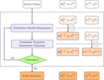
Figure 1: An overview of processes for a typical RANS solver.

With the Boussinesq assumption, the stability is generally not a big issue when the RANS governing equations are solved. However, it becomes much severer if a RANS model beyond the Boussinesq assumption is considered, and convergent solutions may not been obtained at some situations [15, 16], making $\epsilon_{P}$ an important issue that needs to be treated seriously.

Recently, data-driven turbulence modeling has been becoming a promising research field, and many different RANS models have been proposed with the help of different machine learning algorithm [17, 18, 19, 20, 21, 22, 23, 24, 25, 26]. For most data-driven RANS models, no explicit expressions for the Reynolds stress tensor can be obtained [19, 21, 22], and the numerical instability is even severer and $\epsilon_{P}$ could be very large. In Ref. [21], they reported that the mean velocity field obtained with their data-driven RANS model does not match better with the DNS data than the original RANS model, even though their RANS model can predict better Reynolds stresses. In Ref. [15], they believed that RANS equations with explicit data-driven RANS models can be ill-conditioned. In order to make the RANS simulations more stable, they proposed an implicit treatment. With the information of the strain-rate tensor from the DNS database, this implicit treatment can also reduce $\epsilon_{P}$ to a very low level. Nevertheless, the consistent and accurate strain-rate tensor is not always known in advance, which limits the usage of this implicit treatment.

On the other hand, it has been shown by Thompson et al. [27] that the error of solving RANS equations with Reynolds stresses from accurate DNS can still be very large. With friction Reynolds number $Re_{\tau}=5200$ in turbulent channel flow, a $0.41\%$ maximum error in turbulent shear stresses could finally lead to a $21.6\%$ volume-averaged error in the mean velocities [27, 15]. In Ref. [19], they also reported that their predicted streamwise velocity using true DNS anisotropy behaves differently from that from the true DNS (Figure 5 in Ref. [19]). From these results, we may conclude that $\epsilon_{P}$ could be very large if the RANS governing equations (1) and (2) are not solved properly.

The present paper aims to study the propagation error $\epsilon_{P}$ when the mean flow fields are solved with known Reynolds stresses. The Reynolds stresses obtained from DNS are adopted to minimize the influence of $\epsilon_{M}$.

2 Methodology

2.1 Implicit treatment with known $R_{ij}^{DNS}$ and $S_{ij}^{DNS}$

Firstly, let’s consider the momentum equation appeared in (2) at steady state. With the deviatoric anisotropic part of Reynolds stress tensor $a_{ij}=\langle u_{i}u_{j}\rangle-2k\delta_{ij}/3$ and an alternative pressure $\tilde{P}=p/\rho+2k/3$, the momentum equation can be rewritten as

$$U_{j}\frac{\partial U_{i}}{\partial x_{j}}=-\frac{\partial\tilde{P}}{\partial x_{i}}+\nu\frac{{\partial}^{2}U_{i}}{\partial x_{j}\partial x_{j}}-\frac{\partial a_{ij}}{\partial x_{j}}.$$ (4)

As shown in Ref. [15], if the above equation (4) was directly solved with iterative CFD solvers, the local conditioning number could be very large for the corresponding linear algebraic system, making it very difficult to obtain a stable converged solution for equation (4). With known $R_{ij}^{DNS}$ and $S_{ij}^{DNS}$ from the DNS data, Wu et al. [15] proposed an implicit treatment. The basic idea is to decompose $a_{ij}^{DNS}$ into a linear part and a nonlinear part based on eddy-viscosity hypothesis which is written as

$$a_{ij}^{DNS}=-2\nu_{t}S_{ij}^{DNS}+R_{ij}^{\bot},$$ (5)

for incompressible flows. Here,

$$R_{ij}^{\bot}=a_{ij}^{DNS}+2\nu_{t}S_{ij}^{DNS}$$ (6)

is the nonlinear part of the Reynolds stresses, $S_{ij}^{DNS}=(\partial U_{i}^{DNS}/\partial x_{j}+\partial U_{j}^{DNS}/\partial x_{i})/2$ is the mean strain rate tensor from the DNS field, $\nu_{t}$ is the effective turbulence eddy-viscosity, which is the key to quantify and balance the amount of Reynolds stress to be treated implicitly. With the above decomposition (5), the equation (4) can be transformed into

$$U_{j}\frac{\partial U_{i}}{\partial x_{j}} =-\frac{\partial\tilde{P}}{\partial x_{i}}+\frac{\partial}{\partial x_{j}}\left[\left(\nu+\nu_{t}\right)\frac{\partial U_{i}}{\partial x_{j}}\right]-\frac{\partial R_{ij}^{\bot}}{\partial x_{j}}.$$ (7)

Interestingly, although equation (7) is exactly equivalent to equation (4), better stability property can be achieved, which can be explained by the smaller local condition numbers as elucidated by Wu et al. [15], when it is solved numerically with some algorithms (such as SIMPLE algorithm) to obtain its solution $U^{I}_{i}$ as

$$\left(U^{I}_{j}\frac{\partial}{\partial x_{j}}-\frac{\partial}{\partial x_{j}}\left[(\nu+\nu_{t})\frac{{\partial}}{\partial x_{j}}\right]\right)U^{I}_{i}=-\frac{\partial\tilde{P}}{\partial x_{i}}-\frac{\partial R^{\bot}_{ij}}{\partial x_{j}}+E_{N}.$$ (8)

Here, $E_{N}$ is the numerical error when equation (7) is solved, which depends on the numerical schemes, the grid used, the algorithm used to solve the algebraic system and so on. Equivalently, the above equation (8) can be reformed as

$$\left(U^{I}_{j}\frac{\partial}{\partial x_{j}}-\nu\frac{\partial^{2}}{\partial x_{j}\partial x_{j}}\right)U^{I}_{i}=-\frac{\partial\tilde{P}}{\partial x_{i}}-\frac{\partial a_{ij}}{\partial x_{j}}+E_{p}$$ (9)

with

$$E_{p}=\frac{\partial}{\partial x_{j}}\left[2\nu_{t}(S^{I}_{ij}-S^{DNS}_{ij})\right]+E_{N}$$

is the main source of $\epsilon_{P}$. Ideally, if converged solution $U^{I}_{i}$ is obtained and it approaches to $U^{DNS}_{i}$, $\epsilon_{P}$ could be eliminated. However, the inconsistence between $U^{DNS}_{i}$ and $a_{ij}^{DNS}$ as well as the existence of $E_{N}$ makes $\epsilon_{P}$ inevitable. A proper choice of $\nu_{t}$ can reduce $\epsilon_{P}$ to a relatively low level.

2.2 Propagation with known $R_{ij}^{DNS}$ and unknown $S_{ij}^{DNS}$

In the applications of RANS simulations, $R_{ij}$ could generally be obtained through some RANS models while $S_{ij}$ can only be estimated from the current field. With the most accurately estimated $R_{ij}=R_{ij}^{DNS}$ and unknown $S_{ij}^{DNS}$, we still need to find some way to obtain the mean field stably while make $\epsilon_{P}$ as small as possible.

Similar to the decomposition in (5), $a_{ij}^{DNS}$ can still be decomposed with any other known $S_{ij}^{*}$ and $\nu_{t}^{*}$, as

$$a_{ij}^{DNS}=-2\nu_{t}^{*}S_{ij}^{*}+R_{ij}^{\bot*}.$$ (10)

and the corresponding $R_{ij}^{\bot*}$ can be further determined through

$$R_{ij}^{\bot*}=a_{ij}^{DNS}+2\nu_{t}^{*}S_{ij}^{*}.$$ (11)

Since $R_{ij}^{\bot*}$ as well as $S_{ij}^{*}$ can only be determined using the velocity field at the current step, iterations should be adopted to solve the problem, and the numerical solution $U^{n}_{i}$ at the next time step satisfies

$$\left(U^{n}_{j}\frac{\partial}{\partial x_{j}}-\frac{\partial}{\partial x_{j}}\left[(\nu+\nu_{t}^{*})\frac{{\partial}}{\partial x_{j}}\right]\right)U^{n}_{i}=-\frac{\partial\tilde{P}}{\partial x_{i}}-\frac{\partial R^{\bot*}_{ij}}{\partial x_{j}}+E^{n}_{N},$$ (12)

with $R_{ij}^{\bot*}=a_{ij}^{DNS}+2\nu_{t}^{*}S_{ij}^{n-1}$. Here $E^{n}_{N}$ is the numerical error at the $n-th$ step due to the numerical algorithm. Rewriting (12), we have

$$\left(U^{n}_{j}\frac{\partial}{\partial x_{j}}-\nu\frac{\partial^{2}}{\partial x_{j}\partial x_{j}}\right)U^{n}_{i}=-\frac{\partial\tilde{P}}{\partial x_{i}}-\frac{\partial a_{ij}}{\partial x_{j}}+E_{p}^{n}$$ (13)

with

$$E_{p}^{n}=\frac{\partial}{\partial x_{j}}\left[2\nu_{t}^{*}(S^{n}_{ij}-S^{n-1}_{ij})\right]+E^{n}_{N}$$ (14)

being the source of $\epsilon_{P}$ at the $n-th$ step. The final $\epsilon_{P}$ will be determined by all $E_{p}^{n}$ in the past $n$ steps, accumulatively, making both $\nu_{t}^{*}$ and $S_{ij}^{0}$ very important. Again, a choice of $\nu_{t}^{*}$ with larger values can make equation (12) more stable, but it may also increase $E_{p}^{n}$.

Since we only have the information of $a_{ij}$ at the current situation, we need to run some adjoint RANS simulation make a first guess on $\nu_{t}^{*}$ and $S_{ij}^{0}$. With the information of $\nu_{t}^{R}$ and $S_{ij}^{R}$ from the adjoint RANS simulation, we could make some suggestions on $S_{ij}^{0}=S_{ij}^{R}$ and $\nu_{t}^{*}$, either

$$\nu_{t}^{*}=\nu_{t}^{R},$$ (15)

or

$$\nu_{t}^{*}=-\frac{1}{2}\frac{a_{ij}S_{ij}^{R}}{S_{ij}^{R}S_{ij}^{R}}.$$ (16)

In the following, the above two choices will be denoted as algorithm A1 and A2 respectively. Details of these two methods are summarized in Algorithm 1 and Algorithm 2.

1 Run baseline RANS simulation to obtain $S_{ij}^{RANS}$ and $\nu_{t}^{RANS}$ ;

2 Set $\nu_{t}^{*}=\nu_{t}^{RANS}$, $S_{ij}^{*}=S_{ij}^{RANS}$ ;

3 Obtain $R_{ij}^{\bot*}$ through (11) ;

4 for $(k=0;k<N;k++)$ do

5       Solve equation (12) to get intermediate velocity fields $U_{i}^{(k)}$ ;

6       Calculate $S_{ij}^{(k)}$ through $U_{i}^{(k)}$ ;

7       Update $R_{ij}^{\bot*}=a_{ij}^{DNS}+2\nu_{t}^{RANS}S_{ij}^{(k)}$

8 end for

Algorithm 1 Baseline RANS Correction (A1)

1 Run baseline RANS simulation to obtain $S_{ij}^{RANS}$ and $\nu_{t}^{RANS}$ ;

2 Set $S_{ij}^{*}=S_{ij}^{RANS}$ ;

3 Obtain $\nu_{t}^{*}$ through (16) ;

4 Obtain $R_{ij}^{\bot*}$ through (11) ;

5 for $(k=0;k<N;k++)$ do

6       Solve equation (12) to get intermediate velocity fields $U_{i}^{(k)}$ ;

7       Calculate $S_{ij}^{(k)}$ through $U_{i}^{(k)}$ ;

8       Update $\nu_{t}^{m*}=-\frac{1}{2}\frac{a_{ij}^{DNS}S_{ij}^{(k)}}{S_{ij}^{(k)}S_{ij}^{(k)}}$ ;

9       Update $R_{ij}^{\bot*}=a_{ij}^{DNS}+2\nu_{t}^{m*}S_{ij}^{(k)}$ ;

10      

11 end for

Algorithm 2 Maximum Linearization (A2)

3 Numerical results

In this section, the above proposed two different algorithms will be tested numerically in the flow over two-dimensional (2D) periodic hills, where flow separation and reattachment occur on a smooth curved boundary surface. Due to its relatively simple geometry and well-defined boundary conditions [28, 29, 30, 31], it has often been used as benchmark test cases for modeling and simulation issues, such as subgrid-scale models and wall functions in LES [29, 32, 33], data-driven turbulence modeling [21, 22, 34]. A sketch of basic geometry is shown in Figure  2. The streamwise and vertical directions are denoted as $x$ and $y$ respectively. The Reynolds number is defined based on the hill height $h$ and the bulk velocity $U$ at inflow section, $Re=Uh/\nu$ with $\nu$ the kinematic viscosity. The hill length is denoted by $L_{h}$ and the length of flat part of bottom wall is denoted by $L_{f}$. An accurate specification for hill shape is available in form of piece-wise polynomials in [28, 31].

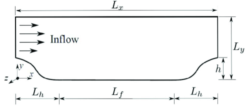
Figure 2: A sketch of computational domain for flow over 2D periodic hills. The hill height is denoted by $h$. The total length and height of the whole domain are denoted by $L_{x}$ and $L_{y}$ respectively.

A 2D structured grid is adopted with resolution $128\times 160$ in streamwise and normal direction. The grid is refined in the near wall region to ensure that the height of the first cell center above the wall in wall unit is less than 1 for all cases and the grid independence has been checked. All RANS simulations are conducted via the steady-state solver ”simpleFoam” based on SIMPLE algorithm (for Semi-Implicit Method for Pressure-Linked Equations) [35] from the widely used open-source platform OpenFOAM [36]. The flow is set to be periodic in the streamwise direction. No-slip condition and zero-gradient condition are set at walls for velocity field and pressure respectively.

As the first test, we would like to show the results of the two algorithms at $Re=10595$ with the Spalart-Allmaras model [5] as the adjoint RANS model. The DNS data of Reynolds stress fields are referred to Breuer et al. [30]. The ratio $\sigma\equiv\delta U_{rms}/U_{rms}^{DNS}$ is used to quantify the error of solved mean velocity field to the reference DNS field, where $\delta U_{rms}$ and $U_{rms}^{DNS}$ are defined as [15]

$$\delta U_{rms}=\sqrt{\frac{\sum_{j=1}^{N}\left([U]_{j}-\left[U^{DNS}\right]_{j}\right)^{2}\left[\Delta V_{j}\right]}{V}}$$ (17)

$$U_{rms}^{DNS}=\sqrt{\frac{\sum_{j=1}^{N}\left(\left[U^{DNS}\right]_{j}\right)^{2}\left[\Delta V_{j}\right]}{V}}.$$ (18)

Here, $[\phi]_{j}$ denotes the $j$-th component of the $N$-vector obtained by discretizing the field $\phi$ on the $N_{x}\times N_{y}$ mesh with $N=N_{x}\times N_{y}$.

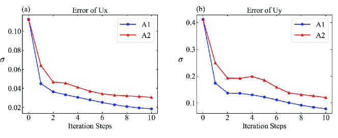
Figure 3: Errors of propagated velocity for $Re=10595$ at different iteration steps with SA model as the adjoint RANS model via algorithms $A1$ and $A2$: (a) streamwise velocity $U_{x}$ and (b) vertical velocity $U_{y}$. The corresponding errors for $U_{x}$ and $U_{y}$ using known $S_{ij}^{DNS}$ are about 0.0083 and 0.042 respectively.

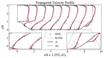
Figure 4: Propagated streamwise velocity profiles on 9 separated locations for $Re=10595$ from the algorithms $A1$ and $A2$. The DNS data and RANS-SA results are also shown for comparison.

Figure 3 shows the errors of streamwise and vertical mean velocities for $Re=10595$ with SA model as the adjoint RANS model via two algorithms as the iteration advances. It is seen that the errors of two velocity components from algorithm $A1$ and $A2$ generally decrease with the iteration advances. They decay very fast during the first two iterations and then become slowly if the iteration goes on. The errors from algorithm $A1$ is lower than those from algorithm $A2$. For $U_{x}$ and $U_{y}$, $\sigma$ are about $0.018$ and $0.078$ for algorithm $A1$ while they are about $0.031$ and $0.120$ for algorithm $A2$ after 10 iterations. Comparing to the corresponding errors from the propagation with $S_{ij}^{DNS}$, which are $0.0083$ and $0.042$, the errors for algorithm $A1$ are about twice while those for algorithm $A2$ are about four or three times. Considering that algorithm $A1$ and $A2$ do not need the information about $S_{ij}^{DNS}$, the present increase in errors is acceptable. Furthermore, the errors from baseline RANS, which are about $0.113$ and $0.412$, are one order of magnitude larger than those with correct Reynolds stresses. In order to further show the differences among different results, the mean streamwise velocity profiles from two different algorithms, as well as those from DNS and baseline RANS simulations, at 9 different locations are shown in Figure 4. Firstly, it is seen that the baseline RANS with SA model fails to predict the mean velocity profiles at the 9 locations as compared to the reference DNS profiles. Fictitious backflows can still be observed even at $x/h=6$ for RANS-SA simulation. It is interesting to note that although the baseline RANS predict the mean velocity very poorly, it still can help to promote the prediction of the algorithm $A1$ and $A2$ as shown in Figure 4, where the mean streamwise velocity profiles at 9 different locations match very well with the DNS data. Compared to the baseline RANS simulations, the algorithm $A1$ has the same eddy viscosity besides the additional nonlinear Reynolds stresses. The better prediction on the mean velocities of the algorithm $A1$ over the baseline RANS then well documents the importance of the nonlinear part of the Reynolds stresses in this kind of flow problems with separations and reattachments. The algorithm $A2$ also can get a very good prediction on the mean velocity profiles, although a little poorer than the algorithm $A1$. This results then illustrates that the choice of $\nu_{t}$ will influence the final results to a certain degree.

4 Discussions

4.1 Influence of adjoint RANS models

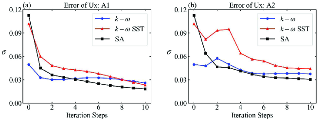
Figure 5: Errors of propagated velocity $U_{x}$ using $A1$ (a) and $A2$ (b) with different adjoint RANS models at $Re=10595$.

Since the choice of $\nu_{t}$ will affect the final results, the different choice of adjoint RANS models will surely affect the final results. Figure 5 shows the errors of $U_{x}$ using $A1$ and $A2$ with three different adjoint RANS models, including the SA model, the $k$-$\omega$ model [13] and the $k$-$\omega$ SST model [37]. It is seen that both algorithms $A1$ and $A2$ can effectively reduce the errors to a relatively lower level, as compared to the errors of baseline RANS simulations, i.e. the errors at the $0-th$ iteration, although they are different for different models. Clearly, $A1$ is more stable than $A2$ and its errors are also smaller, again confirms that $A1$ is better than $A2$. We also tested the two algorithms at different geometries and different Reynolds numbers (not shown here), and the results showed that $A1$ is more stable than $A2$, with smaller errors.

4.2 Other possible approaches

In the above discussions, we have shown that setting $\nu_{t}^{*}=\nu_{t}^{R}$ can generally reduce $\epsilon_{P}$ to a lower level. However, from equations (13) and (14), other choices could still be adopted. For example, we could set

$$\nu_{t}^{*}=C\nu_{t}^{R}$$

where $C$ is a constant in the whole domain, which can be constant or changing during iterations. For SA model, $C\approx 0.7$ could get a slightly better prediction on the mean velocity field. However, we could not determine $C$ in advance without testing which surely will restrict its implementations.

Another choice is to include the history effect when estimates $R_{ij}^{\bot*}$ at the $n-th$ step, such as

$$R_{ij}^{\bot(n)}=a_{ij}^{DNS}+2\nu_{t}^{*}[S_{ij}^{n}+\alpha(S_{ij}^{n}-S_{ij}^{n-1})].$$

or we could use the adaptive gradient algorithm [38] or “Adam” algorithm [39] to make a better estimation on $R_{ij}^{\bot*}$. However, based on our numerical tests, we can only lower the error a little bit.

5 Conclusions

In traditional RANS simulations, the propagation error $\epsilon_{P}$ of obtaining the mean fields with known Reynolds stresses was usually misinterpreted as a part of the modelling error, and has seldom been discussed alone. This makes the judgement on the turbulence models very ambiguous, especially for the data-driven turbulence models which are very popular nowadays. In the present paper, we studied the propagation error $\epsilon_{P}$ solely by using the Reynolds stresses from DNS databases, and the sources of $\epsilon_{P}$ was derived for the situations with or without known $S_{ij}^{DNS}$. For general implementations without known $S_{ij}^{DNS}$, the choice of $\nu_{t}^{*}$ is very critical. If it is too small, the numerical algorithm may be unstable which will increase the error due to the numerical algorithm. On the other hand, if it is too large, it will increase the iteration errors during two adjacent iterations instead. An adjoint RANS simulation was suggested to make a first guess on $\nu_{t}^{*}$ and a good, stable choice is setting $\nu_{t}^{*}$ to the eddy viscosity from RANS simulations. With around ten iterations, the error of mean velocity could be reduced by one-order of magnitude. The present work may offer some valuable references for turbulence models beyond the Boussinesq assumption to obtain satisfactory mean velocity fields.

Another outcome of the present work is on the modelling issues. The Algorithm $A1$ can be viewed as a nonlinear correction to the adjoint linear eddy-viscosity RANS model. The better prediction using $A1$ on the mean velocity fields over the baseline RANS model confirms the importance of non-linear part Reynolds stresses, especially for the current type of flow problems with flow separations. This may be helpful for the those groups who are trying to develop advanced data-driven turbulence models.

Disclosure statement

No potential conflict of interest was reported by the author(s).

Funding

Guo, Xia and Chen is supported by the National Science Foundation of China (NSFC grant nos. 11822208, 11772297, 91852205 and 91752202). Xia is also supported from the Fundamental Research Funds for the central Universities.

References

- [1] Chou PY. On an extension of Reynolds’ method of finding apparent stress and the nature of turbulence. Chin J Phys. 1940;4:1–33.
- [2] Kolmogorov AN. The equations of turbulent motion in an incompressible fluid. Izvestia Acad Sci, USSR; Phys. 1942;6:56–58.
- [3] Chou PY. On velocity correlations and the solutions of the equations of turbulent fluctuation. Quart Appl Math. 1945;3:38–54.
- [4] Baldwin B, Lomax H. Thin-layer approximation and algebraic model for seperated turbulent flows. AIAA Paper 78-257; 1978.
- [5] Spalart PR, Allmaras SR. A one-equation turbulence model for aerodynamic flows. Rech Aerosp. 1994;1:5–21.
- [6] Jones W, Launder B. The prediction of laminarization with a two-equation model of turbulence. Int J Heat Mass Trans. 1972;15(2):301–314.
- [7] Launder B, Sharma B. Application of the energy-dissipation model of turbulence to the calculation of flow near a spinning disc. Lett Heat Mass Trans. 1974;1(2):131–137.
- [8] Wilcox DC. Reassessment of the scale-determining equation for advanced turbulence models. AIAA J. 1988;26(11):1299–1310.
- [9] Launder BE, Reece GJ, Rodi W. Progress in the development of a reynolds-stress turbulence closure. J Fluid Mech. 1975;68(3):537–566.
- [10] Speziale CG, Sarkar S, Gatski TB. Modelling the pressure-strain correlation of turbulence: an invariant dynamical systems approach. J Fluid Mech. 1991;227:245–272.
- [11] Pope SB. A more generative effective-viscosity model. J Fluid Mech. 1975;72:331–340.
- [12] Speziale CG. Analytical methods for the development of reynolds-stress closures in turbulence. Annu Rev Fluid Mech. 1991;23(1):107–157.
- [13] Wilcox D. Turbulence modeling for cfd. Third edition ed. DCW Industries; 2006.
- [14] Durbin P. Some recent developments in turbulence closure modeling. Annu Rev Fluid Mech. 2018;50:77–103.
- [15] Wu J, Xiao H, Sun R, et al. Reynolds-averaged navier-stokes equations with explicit data-driven reynolds stress closure can be ill-conditioned. J Fluid Mech. 2019;869:553–586.
- [16] Zhao Y, Akolekar HD, Weatheritt J, et al. Turbulence model development using cfd-driven machine learning ; 2019.
- [17] Parish EJ, Duraisamy K. A paradigm for data-driven predictive modeling using field inversion and machine learning. J Comput Phys. 2016;305:758–774.
- [18] Weatheritt J, Sandberg R. A novel evolutionary algorithm applied to algebraic modifications of the RANS stress cstrain relationship. J Comput Phys. 2016;325:22–37.
- [19] Ling J, Kurzawski A, Templeton J. Reynolds averaged turbulence modelling using deep neural networks with embedded invariance. J Fluid Mech. 2016;807:155–166.
- [20] Duraisamy K, Singh AP, Pan S. Augmentation of turbulence models using field inversion and machine learning. In: AIAA SciTech Forum; 55th AIAA Aerospace Sciences Meeting; 2017. p. 1–18. 2017-0993.
- [21] Wang JX, Wu JL, Xiao H. Physics-informed machine learning approach for reconstructing reynolds stress modeling discrepancies based on dns data. Phys Rev Fluids. 2017;2:034603.
- [22] Wu JL, Xiao H, Paterson E. Physics-informed machine learning approach for augmenting turbulence models: A comprehensive framework. Phys Rev Fluids. 2018;3:074602.
- [23] Zhu L, Zhang W, Kou J, et al. Machine learning methods for turbulence modeling in subsonic flows around airfoils. Phys Fluids. 2019;31(1):015105.
- [24] Duraisamy K, Iaccarino G, Xiao H. Turbulence modeling in the age of data. Annu Rev Fluid Mech. 2019;51(1):357–377.
- [25] Fang R, Sondak D, Protopapas P, et al. Neural network models for the anisotropic reynolds stress tensor in turbulent channel flow. Journal of Turbulence. 2019;0(0):1–19. Available from: https://doi.org/10.1080/14685248.2019.1706742.
- [26] Pandey S, Schumacher J, Sreenivasan KR. A perspective on machine learning in turbulent flows. Journal of Turbulence. 2020;0(0):1–18. Available from: https://doi.org/10.1080/14685248.2020.1757685.
- [27] Thompson RL, Sampaio LEB, de Braganca Alves F, et al. A methodology to evaluate statistical errors in dns data of plane channel flows. Comput Fluids. 2016;130:1–7.
- [28] Almeida G, Durao D, Heitor M. Wake flows behind two-dimensional model hills. Experimental Thermal and Fluid Science. 1993;7(1):87–101.
- [29] Mellen C, Froehlich J, Rodi W. Large eddy simulation of the flow over periodic hills. In: In: Proceedings. 16th IMACS World Congress, Lausanne, Switzerland; 2000.
- [30] Breuer M, Peller N, Rapp C. Flow over periodic hills: Numerical and experimental study in a wide range of reynolds numbers. Comput Fluids. 2009;38:433–457.
- [31] Xiao H, Wu JL, Laizet S, et al. Flows over periodic hills of parameterized geometries: A dataset for data-driven turbulence modeling from direct simulations ; 2019.
- [32] Temmerman L, Leschziner MA, Mellen CP, et al. Investigation of wall-function approximations and subgrid-scale models in large eddy simulation of separated flow in a channel with streamwise periodic constrictions. Int J Heat Fluid Flow. 2003;24(2):157–180.
- [33] Xia Z, Shi Y, Hong R, et al. Constrained large-eddy simulation of separated flow in a channel with streamwise-periodic constrictions. J Turbul. 2013;14(1):1–21.
- [34] Wu JL, Sun R, Laizet S, et al. Representation of stress tensor perturbations with application in machine-learning-assisted turbulence modeling. Comput Methods Appl Mech Engrg. 2019;346:707–726.
- [35] Caretto LS, Gosman AD, Patankar SV, et al. Two calculation procedures for steady, three-dimensional flows with recirculation. In: Cabannes H, Temam R, editors. Proceedings of the Third International Conference on Numerical Methods in Fluid Mechanics; Berlin, Heidelberg. Springer Berlin Heidelberg; 1973. p. 60–68.
- [36] Weller HG, Tabor G, Jasak H, et al. A tensorial approach to computational continuum mechanics using object-oriented techniques. Comput Physics. 1998;12(6):620–631.
- [37] Menter F, Kuntz M, Langtry R. Ten years of industrial experience with the sst turbulence model. Heat and Mass Trans. 2003 01;4:625–632.
- [38] Duchi J, Hazan E, Singer Y. Adaptive subgradient methods for online learning and stochastic optimization. J Machine Learning Res. 2011 07;12:2121–2159.
- [39] Kingma DP, Ba J. Adam: A method for stochastic optimization ; 2014.