Pendant Drop Tensiometry:
A Machine Learning Approach

Abstract

Modern pendant drop tensiometry relies on numerical solution of the Young-Laplace equation and allow to determine the surface tension from a single picture of a pendant drop with high precision. Most of these techniques solve the Young-Laplace equation many times over to find the material parameters that provide a fit to a supplied image of a real droplet. Here we introduce a machine learning approach to solve this problem in a computationally more efficient way. We train a deep neural network to determine the surface tension of a given droplet shape using a large training set of numerically generated droplet shapes. We show that the deep learning approach is superior to the current state of the art shape fitting approach in speed and precision, in particular if shapes in the training set reflect the sensitivity of the droplet shape with respect to surface tension. In order to derive such an optimized training set we clarify the role of the Worthington number as quality indicator in conventional shape fitting and in the machine learning approach. Our approach demonstrates the capabilities of deep neural networks in the material parameter determination from rheological deformation experiments in general.

I Introduction

Tensiometry is a technique to determine the surface or interfacial tensions of a fluid interface. Many tensiometry methods are based on the shape analysis of liquid drops suspended in air or another liquid. Available tensiometric methods include the drop weight method [1, 2, 3, 4] and the oscillating drop method [5, 6]; the by far most frequently used tensiometric technique is the pendant drop method, which is also closely related to the sessile droplet method as both methods rely on the shape analysis of a gravity-deformed droplet based on the Young-Laplace equation. In the pendant drop setup the droplet typically hangs from the tip of a capillary. Variants can include, for example additional spherical particles attached to the droplet [7]. Pendant liquid drops have been investigated extensively since the 18th century, however only in the late 20th century numerical solution techniques made it possible to extract the surface tension from a single picture of a pendant drop with high precision.

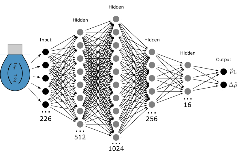
Figure 1: Visualization of the structure of the deep neural network employed for pendant drop tensiometry. The neural network is trained to solve the inverse problem to determine the surface tension (which is contained in the dimensionless density difference $\Delta\tilde{\rho}$) from a pending drop shape.

Before the rise of fast and accessible computer technology the main way to determine interfacial tension from a pendant drop experiment has been the use of precomputed tables in which experimentally accessible dimensionless shape parameters, such as the ratios of the maximum width $D_{E}$ of the droplet and the droplet width $D_{S}$ a distance $D_{E}$ from the apex, are listed with the corresponding interfacial tension [8, 9, 10].

In recent years numerical solution schemes that determine the interfacial tension from the whole droplet profile became more popular and viable solution techniques because of the rapid rise in computers speed [11, 12, 13, 14, 15, 16]. Several implementations exist, where only a single image of a pendant drop and some reference length scale have to be supplied to get a fully automated fit and a surface tension estimate [17, 16, 18]. At the core of this approach is a numerical shape fitting scheme that solves the Young-Laplace shape equations of the drop many times till optimal parameters are found, that provide the best match of the calculated shape to the supplied image. The precision of these methods is often limited by the resolution of the supplied image not allowing for a better fit [16].

The shape fitting problem is, thus, a classical inverse problem of finding a material parameter set that minimizes a suitably defined distance metric between measured and calculated shape. In a Bayesian sense we maximize the likelihood of the material parameters given the measured shape. The forward problem to calculate a droplet shape given the surface tension, gravity, pressure, and the diameter of the capillary can be easily and stably solved by solving the shape equations, which are a set of ordinary differential equations based on the Young-Laplace equation. The corresponding inverse problem of determining the surface tension and pressure given an observed shape is often ill-conditioned if the shape becomes insensitive to parameter changes. In this sense, pendant drop tensiometry is a paradigm for many similar inverse problems in rheology. It has only recently been demonstrated that machine learning approaches can be useful to solve such ill-conditioned inverse problems [19]. To our knowledge, an implementation of a machine learning approach for the pendant drop problem has never been discussed before and offers a novel way to think about the general solution of inverse problems in rheology. So far machine learning applications to rheological problems are limited to solving viscoelastic forward problems with the help of neural networks to replace full finite element calculations [20, 21].

The way a deep neural network learns correlations between input data and output data is especially helpful if a supervised learning scenario can be created. For problems in rheology and physics in general this is often the case, since the forward problem may be sufficiently easy to solve and to compute, the inverse problem, however, can be exponentially hard to solve. Generating a large training set by solving the forward problem many times and training a deep neural network with this data set to learn the necessary correlations to solve the inverse problem can lead to results that even outperform sophisticated conventional shape fitting approaches. Additionally, deep neural networks are lightweight and fast once the network has been trained, which is essential if high-throughput analysis is required. We want to explore the capabilities of a machine learning approach to the inverse Young-Laplace problem as a way to combine the precision of a forward numerical solution scheme with the speed and low hardware demands of a lookup table technique that is working on the entire shape space of droplets and not just a few selected shape parameters.

The article is organized as follows. In Sec. II we first address the underlying physics of pendant drops and present a derivation of the shape equations that a pendant drop needs to fulfill. We also classify all possible pendant drop shapes under pressure and volume control to find the experimentally relevant shapes and the parameter regimes where they exist in nature. Numerically solving the forward problem for the relevant shapes provides the basis for the design and training of a deep neural network that solves the inverse problem to determine the surface tension from a pending drop shape as indicated in Fig. 1. This machine learning approach is presented in Sec. V. Results from conventional shape fitting and machine learning tensiometry are compared in Sec. VI.

II Physics of pendant drops

II.1 Arc length parametrization

A sensible parametrization of an axisymmetric hanging droplet shape is the arc length parametrization for which the first two shape equations can be found by purely geometric arguments:

$$\frac{\mathrm{d}r}{\mathrm{d}s} =\cos\Psi\,,$$ (1)

$$\frac{\mathrm{d}z}{\mathrm{d}s} =\sin\Psi\,,$$ (2)

where we use cylindrical coordinates $(r,z)$ with the $z$-axis as the axis of symmetry and $\Psi$ is the angle of the drop normal with the $z$-axis, see Fig. 2. The principal curvatures in this parametrization are given by the circumferential curvature $\kappa_{\phi}={\sin\Psi}/{r}$ and the meridional curvature $\kappa_{s}={\mathrm{d}\Psi}/{\mathrm{d}s}$.

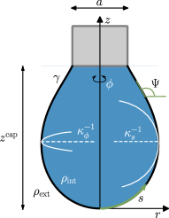
Figure 2: Visualization of a liquid drop in arc length parametrization.

The boundary conditions for a drop hanging from a capillary with diameter $a$ are given by $r(s=0)=0$, $\Psi(s=0)=0$, $z(s=0)=0$ and $r(s=L)={a}/{2}$, where $L$ is the total length of the arc. The boundary conditions at $s=0$ describe the apex of the drop, where the radius, the arc angle and the height are fixed to zero. Only the last boundary condition at $s=L$ describes the attachment to the capillary.

II.2 Young-Laplace equation from local force balance

We consider a droplet with a density difference $\Delta\rho=\rho_{\mathrm{int}}-\rho_{\mathrm{ext}}$ across the interface, attached to the capillary and pulled down by gravity. The problem can be discussed for given Laplace pressure $p_{\mathrm{L}}$ at the apex of the drop or prescribed drop volume $V$. For prescribed drop volume, $p_{\mathrm{L}}$ is introduced as a Lagrange multiplier to fulfill the volume constraint. In both cases the Young-Laplace equation follows from a vanishing first variation of the droplet energy which is a necessary condition that stationary droplet shapes have to fulfill.

There are several ways to derive the Young-Laplace equation based on the concept of energy minimization or, equivalently, local force balance. Here, we consider the forces along the $z$-axis. We cut the drop at height $z$ and consider the $z$-components of the total forces on the lower part of the drop. There are four forces acting on every horizontal slice of the drop, the surface tension force component in $z$-direction $F_{\gamma}^{z}$, the pressure force $F_{p}$, the gravitational force $F_{g}$ caused by the mass hanging below height $z$ and the buoyancy force caused by the difference in density $F_{B}$

$$F_{\gamma}^{z}(z) =2\pi r(z)\gamma\sin\Psi$$ (3)

$$F_{p}(z) =-p(z)\pi r^{2}(z)$$ (4)

$$F_{g}(z)+F_{B}(z) =-\Delta m(z)g$$ (5)

with

$$\Delta m(z)=\pi\Delta\rho\int_{0}^{z}\mathrm{d}z^{\prime}r^{2}(z^{\prime})\,,$$ (6)

the mass difference below height $z$ and the hydrostatic pressure $p(z)=p_{\mathrm{L}}-\Delta\rho gz$, where $p_{\mathrm{L}}$ is the pressure at the apex of the drop. The force balance condition then states at any height $z\in[0,z^{\mathrm{cap}}]$:

$$p(z)\pi r^{2}(z)=2\pi r(z)\gamma\sin\Psi-m(z)g\,.$$ (7)

Taking the derivative ${\mathrm{d}}/{\mathrm{d}z}$ on both sides

$$\frac{\mathrm{d}}{\mathrm{d}z}\left(r^{2}(z)p(z)\right)=2\gamma\frac{\mathrm{d}}{\mathrm{d}z}\left(\kappa_{\phi}(z)r^{2}(z)\right)-g\rho r^{2}(z)$$

and using

$$\frac{\mathrm{d}\kappa_{\phi}}{\mathrm{d}z} =\frac{\cot\Psi(z)}{r(z)}\left(\kappa_{s}-\kappa_{\phi}\right)$$

$$\frac{\mathrm{d}r}{\mathrm{d}z} =\cot(\Psi)$$

leads to the Young-Laplace equation

$$p(z)=p_{\mathrm{L}}-\Delta\rho gz=\gamma(\kappa_{s}+\kappa_{\phi})\,,$$ (8)

where the interfacial tension $\gamma$, the apex pressure $p_{\mathrm{L}}$, and the density difference across the interface $\Delta\rho$ are constant along the interface. Vice versa, the force balance $F_{\gamma}^{z}(z)+F_{g}(z)+F_{B}(z)+F_{p}(z)=0$ from (7) is a first integral of the Young-Laplace equation. At the apex, we have $\kappa_{s}=\kappa_{\phi}$ by axisymmetry. Therefore, the apex Laplace pressure $p_{\mathrm{L}}$ is experimentally observable via the radius of curvature $R_{0}$ in the apex, $p_{\mathrm{L}}=2\gamma/R_{0}$.

Inserting $\kappa_{s}$ and $\kappa_{\phi}$ as the principal curvatures into (8) leads to the final shape equation of the pendant drop:

$$\frac{\mathrm{d}\Psi}{\mathrm{d}s}=\frac{p_{\mathrm{L}}}{\gamma}-\frac{\Delta\rho gz}{\gamma}-\frac{\sin\Psi}{r}\,.$$ (9)

Shape equation (9) has a numerical singularity at $r(s=0)=0$, which can be circumvented by applying de L’Hôspital’s rule and using the axisymmetry in the apex, yielding the limit $\mathrm{d}\Psi/\mathrm{d}s(s\to 0)\to p_{\mathrm{L}}/2\gamma$.

Solutions to the shape equations with $z(0)=0$ and the attachment boundary condition $r(s=L)={a}/{2}$ will have a variable droplet height $z_{\mathrm{cap}}=z(s=L)$ and, thus, also a variable pressure $p_{\mathrm{cap}}=p_{\mathrm{L}}-\Delta\rho gz_{\mathrm{cap}}$ at the capillary. While the apex pressure $p_{\mathrm{L}}$ is experimentally observable via the apex curvature and a theoretically convenient control parameter, the experimental situation is usually such that the capillary is at a fixed position (i.e., $z_{\mathrm{cap}}$ is fixed) and, if working under pressure control, the capillary pressure $p_{\mathrm{cap}}$ is controlled rather than the apex pressure $p_{\mathrm{L}}$.

II.3 Non-dimensionalization and control parameters

We choose the length scale $a$ for non-dimensionalization as the diameter of the capillary leading to the definitions $\tilde{z}\equiv{z}/{a}$, $\tilde{r}\equiv{r}/{a}$, $\tilde{s}\equiv{s}/{a}$, and $\tilde{\kappa}_{s,\phi}\equiv{\kappa_{s,\phi}}{a}$. The non-dimensional form of the Young-Laplace equation (8) is given by

$$\tilde{p}_{\mathrm{L}}-\Delta\tilde{\rho}\tilde{z} =\tilde{\kappa}_{s}+\tilde{\kappa}_{\phi}~{}~{}\mbox{with}$$ (10)

$$\tilde{p}_{\mathrm{L}} \equiv\frac{p_{\mathrm{L}}a}{\gamma}~{}~{}\mbox{and}~{}~{}\Delta\tilde{\rho}\equiv\frac{\Delta\rho ga^{2}}{\gamma},$$ (11)

where we introduced the non-dimensional apex pressure $\tilde{p}_{\mathrm{L}}$ and the non-dimensional gravitational control parameter $\Delta\tilde{\rho}$.

Note that setting the length scale for non-dimensionalization to the radius of curvature in the apex of the drop $R_{0}$ further eliminates the non-dimensional apex pressure from the system of differential equations, since ${p_{\mathrm{L}}R_{0}}/{\gamma}=2$, leading to the often used definition of the bond number [16, 22, 9, 23]

$$\mathrm{Bo}=\frac{\Delta\rho gR_{0}^{2}}{\gamma}=\frac{4\Delta\rho g\gamma}{p_{\mathrm{L}}^{2}}$$ (12)

as a single non-dimensional control parameter. For free-standing droplets without attachment to a capillary the bond number $\mathrm{Bo}$ is the only shape control parameter. As soon as an attachment boundary condition, e.g., $r(s=L)={a}/{2}$, is applied a second control parameter must be defined, which involves the attachment length scale $a$. When using $R_{0}$ for non-dimensionalization this additional control parameter is hidden in the attachment boundary condition itself. We choose the non-dimensionalization length scale $a$ such that the attachment boundary condition is parameter-free and, thus, get the Laplace pressure $\tilde{p}_{\mathrm{L}}$ in the apex and the dimensionless density difference $\Delta\tilde{\rho}={\Delta\rho ga^{2}}/{\gamma}$, which can also be interpreted as a dimensionless measure for the square of the capillary diameter, as two independent non-dimensional shape control parameters. For water droplets in air with $\gamma=72{\rm mN/m}$, a value $\Delta\tilde{\rho}=1$ corresponds to a capillary diameter of $a=2.7{\rm mm}$.

Note that we limit our focus to pendant drops, so $\Delta\tilde{\rho}$ is always positive. When considering setups where the drop rises from a capillary $\Delta\tilde{\rho}$ can also be negative.

From fitting the pendant drop shape (either conventionally or by machine learning) we will obtain a guess for the two dimensionless parameters $\tilde{p}_{\mathrm{L}}$ and $\Delta\tilde{\rho}$. If pressure is not measured in the experiment, the surface tension has to be extracted from the parameter $\Delta\tilde{\rho}$ for known density contrast $\Delta\rho$ and capillary diameter $a$. In this sense, $\Delta\tilde{\rho}$ is the more important parameter to determine. From the second parameter $\tilde{p}_{\mathrm{L}}$, we can then obtain a measurement of the actual apex pressure.

II.4 Droplet shapes classified by bulges and necks

We will discuss droplet shapes either under apex pressure control (parameter $\tilde{p}_{\mathrm{L}}$) or under volume control (with $p_{\mathrm{L}}$ as a Lagrange multiplier). Even these two non-dimensional shape control parameters are not sufficient to fully characterize the pendant drop’s shape. The Young-Laplace equation with height-dependent hydrostatic pressure (8) has no closed analytical solutions; solutions for pendant drops are distorted unduloids [24]. An unduloid is an axially symmetric constant mean curvature surface with a curvature ratio $|\kappa_{s}/\kappa_{\phi}|<1$. This curvature condition is also fulfilled for the droplet profiles, but the mean curvature is decreasing for $z>0$ because of the decreasing hydrostatic pressure $p(z)$. Therefore, similarly to an unduloid, the droplet profile radial distance function $\tilde{r}(\tilde{s})$ contains several maxima (bulges) and minima (necks) for larger $\tilde{p}_{\mathrm{L}}$, such that the attachment boundary condition may be fulfilled at a number of different total dimensionless arc lengths $\tilde{L}$ along the same solution of the shape equations leading to different shapes for the same choices of $\tilde{p}_{\mathrm{L}}$ and $\Delta\tilde{\rho}$. This gives rise to several possible classes of solution shapes which can be characterized by their number of bulges and necks and the first three of which are shown in Fig. 3. The number of bulges and necks is counted by another discrete parameter

$$\Omega\equiv 1+\#\mathrm{necks}+\#\mathrm{bulges}$$ (13)

that indicates the class of a solution.

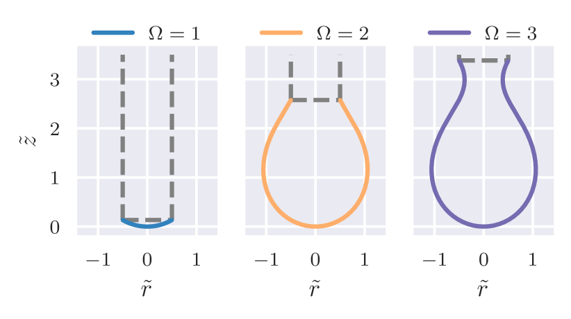
Figure 3: Comparison of valid solution shapes for solution classes $\Omega\in\{1,2,3\}$ for parameters: $\tilde{p}_{\mathrm{L}}=2$, $\Delta\tilde{\rho}=0.3$. The dashed grey lines indicate the capillary. Higher class solutions always contain the shapes of all lower class solutions, since all classes are constructed from the same general solution shape that is cut off at different heights.

The first class of solutions, $\Omega=1$, is a simple convex shape with $\tilde{r}(\tilde{s})<{1}/{2}$ for all $0\leq\tilde{s}<\tilde{L}$; this class has a monotonically increasing radius with $\tilde{r}(\tilde{s}=0)=0$ in the apex and $\tilde{r}(\tilde{L})={1}/{2}$ at the capillary.

The second class of solutions, $\Omega=2$, are convex shapes for which there exists exactly one bulge, where we define a bulge as a point where $\tilde{r}(\tilde{s})$ has a local maximum (such that $\sin\Psi(\tilde{s})=1$ see (1)). The $\Omega=2$ shapes are convex and always bulge out, i.e., the bulge is wider than the capillary. The shape class $\Omega=2$ will be the most important class for shapes under volume control.

The third solution class, $\Omega=3$, is the first class of non-convex solutions. These solutions have exactly one bulge and one neck, where a neck is defined as a point where $\tilde{r}(\tilde{s})$ has a local minimum (such that also $\sin\Psi(\tilde{s})=1$, see (1)). The $\Omega=3$ solutions have a neck at the capillary and always cross the capillary boundary condition from left to right, i.e., ${\mathrm{d}\tilde{r}(\tilde{s})}/{\mathrm{d}\tilde{s}}\rvert_{\tilde{s}=\tilde{L}}\geq 0$.

Continuing this scheme there also exist higher classes $\Omega>3$ of shapes, in principle, which are characterized by their increasing number of bulges and necks. While all shape classes up to $\Omega=3$ can actually be observed in experiments, higher classes $\Omega>3$ are not observed because they are energetically unfavorable and unstable both under volume and pressure control as we will show in the next section.

II.5 Shape bifurcations and shape diagram for pendant drops

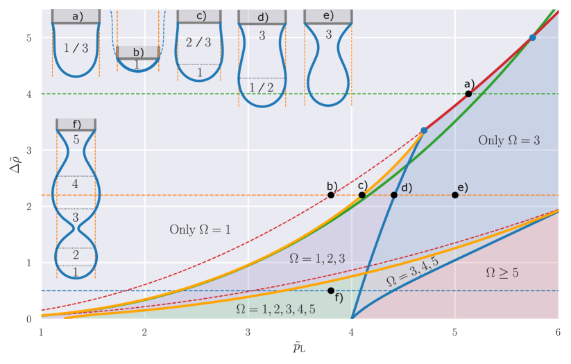
Figure 4: Shape diagram in the $\tilde{p}_{\mathrm{L}}$-$\Delta\tilde{\rho}$ parameter plane for apex pressure control. Shapes corresponding to black points in parameter space are shown on the right. At the yellow lines two additional droplet shapes $\Omega=n+1,n+2$ appear, at the blue lines two droplet shapes $\Omega=n,n+1$ annihilate in bifurcations ($n=1,3,...$). Blue and yellow lines terminate in a critical point at $\Delta\tilde{\rho}=3.37$ for $n=1$ and $\Delta\tilde{\rho}=2.07$ for $n=3$. At the red lines shapes develop saddle points; the lower pointed part of the red line is not observable as the saddle develops in the continuation of the shape to the region above the capillary opening and outside the capillary. At the green line, the maximal volume is reached for increasing pressure. Droplets detach at this line, either in shape $\Omega=1$ for $\Delta\tilde{\rho}>5.02$ or in shape $\Omega=3$ for $\Delta\tilde{\rho}<5.02$. Example shapes a)-e) illustrating the bifurcations are shown for $\Delta\tilde{\rho}=4$ (green dashed line, shape a), $\Delta\tilde{\rho}=2.2$ (yellow dashed line, shapes b-e), and $\Delta\tilde{\rho}=0.5$ (blue dashed line, shape f).

For the tensiometry analysis, we first discuss where the different shape classes can be found in the $\tilde{p}_{\mathrm{L}}$-$\Delta\tilde{\rho}$ parameter plane under pressure control and in the $\Delta\tilde{\rho}$-$\tilde{V}$ parameter plane under volume control, which leads to the shape diagrams Figs. 4 and 5. This will be important for identifying the experimentally relevant parameter regions and to rationalize parameter sensitivity of shapes and the selection of the relevant shapes for the training of the neural network.

We will first discuss all possible shapes under apex pressure control. This means we integrate the shape equations (1), (2), and (9) in dimensionless form starting at the apex with given $\tilde{p}_{\mathrm{L}}$ and $\Delta\tilde{\rho}$ and ignoring the attachment boundary condition at the capillary. At every intersection with the capillary, where $\tilde{r}(\tilde{s})=1/2$, the remaining attachment boundary condition can be fulfilled with a different arc length. This means for a solution which intersects $n$-times with the capillary, all shape classes $\Omega=1,...,n$ can occur in the shape diagram for this choice of parameters.

For small pressure, there is only one intersection and only shapes with $\Omega=1$ exist. For increasing apex pressure $p_{\mathrm{L}}$ the curvature of droplet shapes increases and higher order shapes $\Omega>1$ with more bulges and necks become possible in a sequence of bifurcations, which are shown in the bifurcation diagram Fig. 4.

We follow the sequence of bifurcations for fixed $\Delta\tilde{\rho}$ and increasing apex pressure $p_{\mathrm{L}}$. In a first simple fold bifurcation a bulge and neck pair is formed via a saddle point configuration of the droplet. At this bifurcation, an $\Omega=n$ shape transforms into an $\Omega=n+2$ shape. The first bulge/neck pair is formed at the left red bifurcation line in the shape diagram Fig. 4 (transition $\Omega=1\to 3$); higher order lines exist but are not shown. We find numerically that the red dotted bifurcation lines are parabolas with $\Delta\tilde{\rho}\simeq 0.15\,\tilde{p}_{\mathrm{L}}^{2}$ and $\Delta\tilde{\rho}\simeq 0.054\,\tilde{p}_{\mathrm{L}}^{2}$.

There is a critical value $\Delta\tilde{\rho}_{\mathrm{c1}}\simeq 3.37$, where the first saddle forms exactly at the capillary radius $\tilde{r}=1/2$. For $\Delta\tilde{\rho}>3.37$ the first saddle forms at a radius smaller than the capillary radius (at $\tilde{r}<1/2$, see Fig. 4, shape a), for $\Delta\tilde{\rho}<3.37$ it would form above the capillary opening and “outside” the capillary (see Fig. 4, shape b), i.e., the saddle would form in the region $\tilde{r}(s)>1/2$ and for $s>L$ above the only possible attachment point to the capillary, where $\tilde{r}(L)=1/2$). Therefore, the bifurcation at the red line is unobservable in an actual experiment for $\Delta\tilde{\rho}<3.37$ (dotted red line). Likewise, there is a critical value $\Delta\tilde{\rho}_{\mathrm{c2}}\simeq 2.07$ for the formation of the second saddle, and for $\Delta\tilde{\rho}>2.07$ the second saddle forms inside the capillary, while it forms above and outside for $\Delta\tilde{\rho}<2.07$ (dotted red line). These critical values also exist for the higher order lines, in principle. The critical values $\Delta\tilde{\rho}_{\mathrm{c1}}\simeq 3.37$ and $\Delta\tilde{\rho}_{\mathrm{c2}}\simeq 2.07$ define critical points on the respective bifurcation lines. Because a saddle configuration has vanishing curvature $\kappa_{s}=0$, a saddle configuration right at the capillary has a capillary Laplace pressure $\tilde{p}_{\mathrm{cap}}=\tilde{\kappa}_{\phi}=2$, which is thus the capillary pressure for all critical points.

For capillary widths smaller than the critical values ($\Delta\tilde{\rho}<3.37$ for the first bulge/neck pair or $\Delta\tilde{\rho}<2.07$ for the second), bifurcations occur only after a bulge/neck pair has formed “outside” the capillary (at $\tilde{r}>1/2$). Then bulge and neck “move inwards” towards the symmetry axis upon increasing the pressure further, and droplet shapes bifurcate if a neck moves inwards and touches the capillary radius (i.e., the neck is at $\tilde{r}=1/2$, see shape c in Fig. 4). Coming into this bifurcation with the highest possible shape $\Omega=n$ ($n=1,3,...$ odd), a pair $\Omega=n+1,n+2$ of additional shapes become possible in a simple fold bifurcation (at the yellow bifurcation lines in the shape diagram Fig. 4, illustrated for $n=1$ with shape c). Right at these bifurcation lines, both shapes $\Omega=n+1,n+2$ are identical and the droplet has a vertical tangent at the capillary.

Likewise, if a bulge moves inwards and touches the capillary, a pair $\Omega=n,n+1$ of shapes annihilates again in a simple fold bifurcation (at the blue bifurcation lines in the shape diagram Fig. 4, illustrated for $n=1$ with shape d). Beyond the blue bifurcation lines $\Omega=n+2$ is the lowest possible order of shapes. Right at these bifurcation lines, both shapes $\Omega=n,n+1$ are identical and also have a vertical tangent at the capillary. As a result, in the magenta and green shaded areas between the yellow and blue bifurcation lines, classes $\Omega=1,2,3$ are possible, in the green and grey shaded areas classes $\Omega=3,4,5$ are possible, and so on (see shape f in Fig. 4).

At the first blue bifurcation line, where shapes $\Omega=1,2$ annihilate, these shapes are approximately half-spherical (see shape d in Fig. 4). They are exactly half-spherical for $\Delta\tilde{\rho}=0$ with radius $\tilde{R}_{0}=2/\tilde{p}_{\mathrm{L}}=1/2$, and volume $\tilde{V}=\pi/12$. Along the blue bifurcation line, the maximal dimensionless Laplace pressure increases to $\tilde{p}_{\mathrm{L}}>4$ for $\Delta\tilde{\rho}>0$, because the shape elongates and the apex acquires a higher curvature.

Both at the yellow and blue bifurcation lines (for example for shapes c and d in Fig. 4), the force equilibrium (7) holds at $z=z_{\mathrm{cap}}$ with $r(z_{\mathrm{cap}})=a/2$ and $\sin\psi=1$ (vertical tangent) resulting in the exact bifurcation condition

$$\Delta\tilde{\rho}\frac{\tilde{V}}{\pi}=1-\frac{\tilde{p}^{\mathrm{cap}}}{4}$$ (14)

which holds along the entire boundary of the magenta, green and grey shaded areas in the shape diagram Fig. 4.

The birth of bulge/neck pairs outside the capillary radius (at the dotted red lines), and their subsequent inward motion with increasing pressure with first the neck crossing the capillary radius (at the yellow bifurcation lines) and then the bulge moving through the capillary radius (at the blue bifurcation lines) explains the structure of the pressure shape diagram Fig. 4 for $\Delta\tilde{\rho}<3.37$, i.e., for sufficiently narrow capillaries. Here we have several possible shape sequences $\Omega=1\to 1,2,3\to...$ (see shapes b to e or shape f in Fig. 4). For $\Delta\tilde{\rho}>3.37$ or wide capillaries, the birth of the first bulge/neck pair inside the capillary radius (at the solid red line, see shape a in Fig. 4) with $\Omega=1\to 3$ is the only bifurcation event.

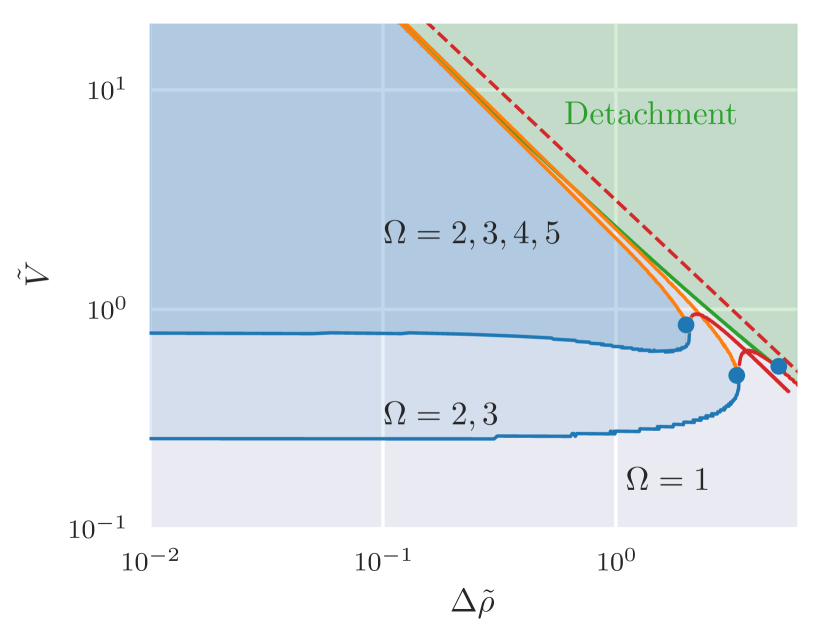
Figure 5: Shape diagram in the $\Delta\tilde{\rho}$-$\tilde{V}$ parameter plane for volume control. At small volumes only shape $\Omega=1$ is possible. Almost up to the detachment volume both shapes $\Omega=2,3$ are possible. Where both shapes (or even higher classes) are possible, the bulged shape $\Omega=2$ is the global energy minimum. Only in a small region close to the maximal volume, the necked shape $\Omega=3$ is the global energy minimum. The upper green line marks the maximal volume, where the droplet detaches. For $\Delta\tilde{\rho}>5.02$ it detaches in shape $\Omega=1$, for $\Delta\tilde{\rho}<5.02$ in the necked shape $\Omega=3$. According to the approximative Tate’s law detachment happens at $\tilde{V}=\pi/\Delta\tilde{\rho}$ (dashed red line);

We can obtain a corresponding volume shape diagram in the $\Delta\tilde{\rho}$-$\tilde{V}$ parameter plane, which is shown in Fig. 5. Again, for $\Delta\tilde{\rho}<3.37$ there are several possible shape sequences $\Omega=1\to 2,3\to...$, whereas for $\Delta\tilde{\rho}>3.37$, there is only one bifurcation $\Omega=1\to 3$ possible.

In the shaded areas in the shape diagrams between the yellow and blue bifurcation lines, several shape classes $\Omega$ are possible. Which shape class is actually assumed because it is stable and energetically favorable and which class is only metastable, depends on the dimensionless energy (measured in units of $a\gamma$)

$$\tilde{F} =\int_{0}^{\tilde{L}}\mathrm{d}\tilde{s}\left(2\pi\tilde{r}(\tilde{s})+\pi\Delta\tilde{\rho}\tilde{z}(\tilde{s})\tilde{z}^{\prime}(\tilde{s})\tilde{r}^{2}(\tilde{s})\right)$$ (15)

of the shape for volume control or the enthalpy

$$\tilde{G} =\tilde{F}-\tilde{p}_{\mathrm{L}}\tilde{V}=\tilde{F}-\tilde{p}_{\mathrm{L}}\pi\int_{0}^{\tilde{L}}\mathrm{d}\tilde{s}\tilde{z}^{\prime}(\tilde{s})\tilde{r}^{2}(\tilde{s})$$ (16)

for apex pressure control. The first term in $\tilde{F}$ is the surface energy, the second term the gravitational energy (measured with respect to the apex $\tilde{z}(0)=0$). At fixed volume, $\tilde{F}$ is minimized in a stationary state, while at fixed apex pressure $\tilde{p}_{\mathrm{L}}$, the enthalpy $\tilde{G}$ is extremized resulting in $\tilde{p}_{\mathrm{L}}=\mathrm{d}\tilde{F}/\mathrm{d}\tilde{V}$. If several shape classes are possible, the shape with the minimal energy $\tilde{F}$ is stable for volume control, while the shape with minimal enthalpy $\tilde{G}$ is stable for apex pressure control.

A shape must have $\mathrm{d}\tilde{p}_{\mathrm{L}}/\mathrm{d}\tilde{V}>0$ to be stable under apex pressure control, otherwise it could increase volume without limit at a given maintained pressure. This implies a convex energy $\tilde{F}(\tilde{V})$ or a concave enthalpy $\tilde{G}(\tilde{p}_{\mathrm{L}})$ as necessary stability condition under pressure control. Stability under volume control can be deduced from the properties of the $\tilde{p}_{\mathrm{L}}(\tilde{V})$-relation using the criteria derived by Maddocks [25]. Thus it is necessary to know the $\tilde{G}(\tilde{p}_{\mathrm{L}})$-, $\tilde{F}(\tilde{V})$-, and $\tilde{p}_{\mathrm{L}}(\tilde{V})$-relations to decide on the stability of shapes.

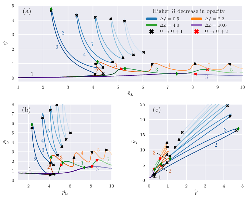
Figure 6: (A) Volume-pressure relationship, (B) enthalpy as a function of pressure, and (C) energy as a function of volume for four shapes with $\Delta\tilde{\rho}=0.5$ (blue) $\Delta\tilde{\rho}=2.2$ (yellow) $\Delta\tilde{\rho}=4.0$ (green), and $\Delta\tilde{\rho}=10.0$ (red). We marked where the bifurcations $\Omega=1\to 1,2,3$ (yellow line in Fig. 4) and $\Omega=1,2,3\to 3$ (blue line in Fig. 4) occur, and the shape of maximal volume.

Therefore, we follow the evolution of all shapes in terms of apex pressure $\tilde{p}_{\mathrm{L}}$, droplet volume $\tilde{V}$ and droplet energy $\tilde{F}$ as well as enthalpy $\tilde{G}=\tilde{F}-\tilde{p}_{\mathrm{L}}\tilde{V}$ through all bifurcations in Fig. 6 for the four values $\Delta\tilde{\rho}=0.5,~{}2.2,~{}4.0,~{}10.0$ (also indicated in the shape diagram Fig. 4)). The bifurcation points, where shapes $\Omega=1,2$ vanish and where additional shapes $\Omega=2,3$ appear are marked with black dots, the shape with maximal volume with a green dot.

For $\Delta\tilde{\rho}=4.0,~{}10.0$, i.e., wide capillaries $\Delta\tilde{\rho}>3.37$ there is only a single bifurcation $\Omega=1\to 3$ of the shape upon increasing the pressure, namely, when a bulge/neck pair is created (marked with a red dot in Fig. 6 corresponding to the red line in the shape diagram Fig. 4). Fig. 6 shows that the $\tilde{p}_{\mathrm{L}}(\tilde{V})$-curve is monotonously increasing up to the maximal volume. Therefore shapes $\Omega=1$ and $\Omega=3$ are stable under pressure and volume control up to the shape of maximal volume. The maximal volume shape is attained in a shape $\Omega=3$ for $\Delta\tilde{\rho}=4.0$ but in shape $\Omega=1$ for $\Delta\tilde{\rho}=10.0$.

For $\Delta\tilde{\rho}=2.2$, i.e., in the regime $2.07<\Delta\tilde{\rho}<3.37$ of narrower capillaries, there are two observable bifurcations upon increasing the pressure. Shapes $\Omega=2,3$ appear when a neck appears at the capillary (yellow bifurcation line in Fig. 4), and shapes $\Omega=1,2$ meet and vanish when a bulge appears at the capillary (blue bifurcation line in Fig. 4). Both bifurcations are marked by black dots in Fig. 6. The $\tilde{p}_{\mathrm{L}}(\tilde{V})$-curve is monotonously increasing for shape $\Omega=1$ up to the bifurcation, where shapes $\Omega=1,2$ vanish. In addition, there is an increasing $\tilde{p}_{\mathrm{L}}(\tilde{V})$-curve for shape $\Omega=3$ up to the shape with maximal volume (green dot).

For small $\Delta\tilde{\rho}<2.07$ even five or more shapes can coexist in certain parameter regimes. For $\Delta\tilde{\rho}=0.5$, there is a sequence $\Omega=1\to 3\to 1,2,3\to 3,4,5\to 1,2,3,4,5\to 3,4,5\to 5$ via six bifurcations. The $\tilde{p}_{\mathrm{L}}(\tilde{V})$-curve is monotonously increasing for shape $\Omega=1$ up to the bifurcation, where shapes $\Omega=1,2$ vanish. For all higher shapes the $\tilde{p}_{\mathrm{L}}(\tilde{V})$-curves are almost everywhere decreasing except for very small pieces around the maximal volumes of these shapes.

We conclude that $\Omega=1$ is the only shape which always has an increasing $\tilde{p}_{\mathrm{L}}(\tilde{V})$-relation and is generally stable under pressure and volume control. Under pressure control, shape $\Omega=1$ always has the lowest enthalpy $G$ and is the energetically preferred state where it exists (see Fig.  6(B)). Because the $\tilde{p}_{\mathrm{L}}(\tilde{V})$-curves are S-shaped, we can deduce from the theorems derived by Maddocks [25] that shape $\Omega=2$ is unstable under pressure control but stable under volume control. Under volume control, shape $\Omega=2$ always has the lowest energy and is the energetically preferred state where it exists (see Fig.  6(C)). Shape $\Omega=3$ is stable under pressure and volume control in a small regime from the bifurcation $1\to 1,2,3$ where it appears together with shape 2 up to the maximal volume (green dots in Fig. 6); in this regime it has an increasing $\tilde{p}_{\mathrm{L}}(\tilde{V})$-relation and is the energetically preferred state under volume control. Beyond the shape of maximal volume, shape $\Omega=3$ becomes unstable under pressure control but remains metastable under volume control. Shapes $\Omega\geq 3$ are, however, always energetically unfavorable as higher order shapes have higher energy and enthalpy, as can be seen in Figs. 6(B,C). Under volume control, shapes $\Omega=1,2,3$ are stable up to the maximal volume. All higher order shapes $\Omega\geq 3$ beyond the maximal volume are energetically unfavorable as Figs. 6(B,C) show.

Experimentally, the standard situation is volume control. For this situation the sequence $\Omega=1\to 2\to 3$ is the sequence of energetically preferred states with shape $\Omega=2$ being the global energy minimum in a large volume range (everywhere, where it exists). Therefore, we will focus on the shape classes $\Omega=2,3$ in the tensiometry part of the paper.

II.6 Droplets detach at the maximal droplet volume

The pressure and volume shape diagrams are limited by the maximally possible droplet volume before detachment. From Figs. 6(A,C) it is apparent that, regardless of how complicated the bifurcation sequence might be, there always exists a maximal volume $\tilde{V}_{\mathrm{max}}$ that a pendant drop can accommodate for all values of $\Delta\tilde{\rho}$ (green dots in Fig. 6). This maximal volume marks the end of existence of energetically stable droplet shapes in the diagrams Figs. 6(A,C). This maximal volume is also essential for the stability under gravity. If the droplet is loaded with more than the maximal volume, no stationary state can exist, and the droplet has to start moving downwards by gravity. This leads to gravitational detachment of the droplet, during which it dynamically breaks up into a stable pendant drop of lower volume and a satellite droplet [26, 4], which is the basis of the drop weight method. We only consider stationary droplet shapes and, thus, have only access to the maximal stationary droplet volume before detachment as it has also been used for tensiometry in Ref. 27.

We calculated the shapes of maximal volume numerically and marked them by a green line in the shape diagram in the $\tilde{p}_{\mathrm{L}}$-$\Delta\tilde{\rho}$ plane in Fig. 4. This green line intersects the red line where the bifurcation $\Omega=1\to 3$ occurs via formation of a bulge/neck pair. This intersection happens at a value $\Delta\tilde{\rho}\simeq 5.02$. Therefore, the maximal volume is attained in a shape $\Omega=3$ for narrow capillaries $\Delta\tilde{\rho}<5.02$ and in a shape $\Omega=1$ for wider capillaries $\Delta\tilde{\rho}>5.02$.

For small $\Delta\tilde{\rho}\lesssim 1$ the detachment (green line) happens almost at the same volume as the bifurcation where shapes $\Omega=2,3$ appear (yellow line) as can be seen both in Figs. 4 and 6. In this regime, detachment happens with an almost vertical tangent at the capillary. Therefore, the bifurcation condition (14) also gives an excellent description of the detachment volume in this regime. The similarity to the well-known Tate law is obvious: if we can approximate $\tilde{p}^{\mathrm{cap}}\ll 4$, we recover Tate’s law [1]

$$\tilde{V}\approx\frac{\pi}{\Delta\tilde{\rho}}$$ (17)

for gravitational detachment. In the shape diagram Fig. 5 in the $\Delta\tilde{\rho}$-$\tilde{V}$ parameter plane, Tate’s law is shown as dashed red line, the exact numerical detachment condition is the green line. We clearly see that Tate’s law overestimates the detachment volume leading to the known underestimation of the surface tension by the drop weight method [2, 3]. We also observe in diagram 5 that, for narrow capillaries $\Delta\tilde{\rho}<5.02$, droplets detach in a necked shape $\Omega=3$. while they detach in a simple shape $\Omega=1$ for wider capillaries $\Delta\tilde{\rho}>5.02$.

III Numerical approach

In the following, we study two tensiometry approaches to extract the two control parameters $\tilde{p}_{\mathrm{L}}$ and $\Delta\tilde{\rho}$ from an experimental image of a droplet shape, conventional shape fitting (CSF) as compared to a novel machine learning (ML) approach, where we train a deep neural network to determine the control parameters. To test both methods, we numerically generate droplet shapes with known parameters $\tilde{p}_{\mathrm{L}}$ and $\Delta\tilde{\rho}$ (the “forward problem”) and then re-determine these parameters by shape fitting or by the neural network (the “inverse problem”). From now on we only consider shapes of the classes $2$ and $3$, since they are predominantly used in tensiometry and provide high fitting accuracy in general [16]. We start by only considering class $2$ shapes and discuss the generalized approach to class $2$ and $3$ shapes afterwards. This means we consider shapes in the diagram Fig. 4, which lie in the magenta and green “triangles” enclosed by the yellow and blue bifurcation lines, where shape classes $2$ can exist.

To numerically generate shapes for given parameters $\tilde{p}_{\mathrm{L}}$ and $\Delta\tilde{\rho}$ we make use of a discretization of the shape equations (1), (2), and (9) to solve them iteratively in space. For this a fourth order Runge-Kutta algorithm is used, because it provides a good mix of accuracy and speed. We use a modified version of OpenCapsule [18, 28] for the numerical fitting and forward solution of the Young-Laplace problem. The output data from the numerical forward solution is evenly spaced in the arc lengths $\tilde{s}$ of the shape.

IV Solving the inverse problem by conventional shape fitting

The goal of shape fitting is to numerically generate a shape that has the least square distance to a set of sample points along the contour of an input shape. The numerically generated optimal fit will then make the parameters $\tilde{p}_{\mathrm{L}}$ and $\Delta\tilde{\rho}$ of the input shape available. In CSF, we start with an initial guess for the parameters of the shape $\{\tilde{p}_{L}^{\text{initial}},\Delta\tilde{\rho}_{L}^{\text{initial}}\}$. Second, we determine the Jacobian matrix for the supplied parameters by giving every parameter a notch to either side, comparing the resulting errors and numerically calculating the derivatives this way. Last, the parameters get updated with an update vector that points along the steepest descent in error-parameter space. Generally, this is the way most existing numerical implementations perform the fitting. After some iterations a shape emerges that best fits the points from the contour of the input shape for a pair of best fitting material parameters $\tilde{p}_{\mathrm{L}}$ and $\Delta\tilde{\rho}$.

V Machine learning approach for the inverse problem

A ML approach provides a way to solve the computationally taxing task of numerically fitting the shape in a more efficient way by training the neural networks weights and biases with many training samples in a supervised learning approach. The network fits correlations between the input data and the output labels, i.e., the two parameters $\tilde{p}_{\mathrm{L}}$ and $\Delta\tilde{\rho}$. This correlation can then be used to solve for input never seen before. The main difference to CSF is that we do not directly adjust the parameters $\tilde{p}_{\mathrm{L}}$ and $\Delta\tilde{\rho}$ for each new shape separately, but we rather adjust the weights and biases of the neural network once by training with many shapes and can then obtain parameters $\tilde{p}_{\mathrm{L}}$ and $\Delta\tilde{\rho}$ almost instantly for any new shape without further adjustment. ML has recently been used to solve many complex problems and is growing in popularity among scientists, there is, to our best knowledge, no research showing the capabilities of a ML approach for parameter extraction from shape data of pendant drops. As a ML framework we use Keras [29] and Tensorflow [30].

V.1 Architecture of the network

The architecture of the neural net for pendant drop tensiometry is shown in Fig. 1. The input to the network is essentially the same as the input to the numerical fitting scheme - a discrete set of points along the contour of a drop’s shape. For the ML approach we fix the number of sample points along the shape to a specific sample count $d$, because the input shape of a Dense-Layer has to be of fixed size. The resulting $d\times 2$ input matrix, consisting of the $\tilde{r}$- and $\tilde{z}$-values of the $d$ sample points along the shape, then gets flattened into a $2d\times 1$ input vector. If the input data contains less than $d$ samples the input vector gets zero padded and if the input data contains more than $d$ samples the input is truncated while keeping the apex coordinates. We use a sample count of $d=226$ since an arc length step of $10^{-2}$ between shape point samples gives shapes of class $2$ that generally have less shape sample points than $226$. Increasing the sample count $d$ increases the complexity of the network and will slow the learning process.

The input vector is processed by a fully connected deep neural network with Dense neurons and Leaky-RELU activation functions. The Leaky-RELU activation function aims to fix unwanted behaviour occuring with regular RELU activated neurons by replacing the flat negative region of the RELU function with a linear function that has a finite slope $m\ll 1$ [31].

The first layer has an input dimension of $2d$ and outputs $512$ continuous parameters, the second layer takes the $512$ outputs from the first layer and processes them into $1024$ outputs which the third layer processes into $256$ outputs. The fourth layer has $16$ outputs and finally the fifth layer has $2$ output parameters, which are the fitting parameters $\tilde{p}_{\mathrm{L}}$ and $\Delta\tilde{\rho}$. The layer dimensions emerged from testing and show no overfitting with the training data we use.

V.2 Training of the network

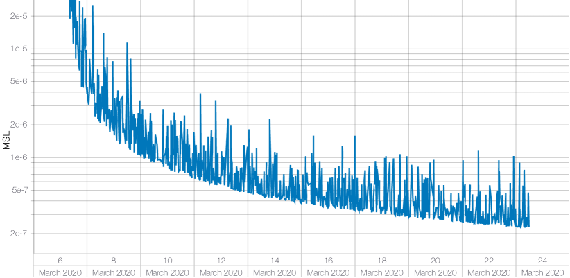
Figure 7: Evolution of the MSE objective function (log-scale) with training time.

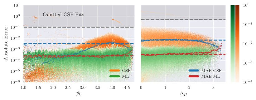
Figure 8: Comparison of the absolute errors for parameters $\tilde{p}_{\mathrm{L}}$ and $\Delta\tilde{\rho}$ between conventional shape fitting and machine learning for class $2$ shapes. The dashed lines indicate the total mean absolute error (MAE) of all fits/guesses and labels. The relevant parameter for the determination of the interfacial tension $\gamma$ is $\Delta\tilde{\rho}$.

The drop shapes for training are generated using the numerical forward solution to the Young-Laplace problem with OpenCapsule. At first, we select training shapes randomly and uniformly selected from the relevant shaded “triangle” enclosed by the yellow and blue bifurcation lines in the shape diagram Fig. 4 in the $\tilde{p}_{\mathrm{L}}$-$\Delta\tilde{\rho}$ plane, where shape classes $2$ and $3$ can exist. This choice of training set aims to obtain a neural network with uniformly good performance in this whole parameter range. An alternative choice of training set will be discussed below.

As a performance metric we pick the mean-square error (MSE) between the output guess and the corresponding labels of the input data. An alternative error metric is the mean absolute error (MAE), which does not penalize rare high amplitude errors as much as MSE does. We train the network with the MSE $\frac{1}{2N}\sum_{n=1}^{N}\left[(\tilde{p}_{\mathrm{L,in,n}}-\tilde{p}_{\mathrm{L,out,n}})^{2}+(\Delta\tilde{\rho}_{\mathrm{in,n}}-\Delta\tilde{\rho}_{\mathrm{out,n}})^{2}\right]$ of $N$ training shapes as an objective function. The network is trained in batches of $N=100$ by backpropagation using the Adadelta [32] gradient descent method with an adaptive learning rate.

During the training period the network was trained for approximately $90,000$ epochs, where one epoch consists of $0.5$ million drop shapes and corresponding parameters $\tilde{p}_{\mathrm{L,inn}}$ and $\Delta\tilde{\rho}_{\mathrm{inn}}$. On standard hardware (i3-CPU with a GTX 970 GPU), this training took approximately 3 weeks, see Fig. 7. The objective function is evaluated with an independent set of $100.000$ shapes between training epochs. The final test set for the error comparison (see next section) comprises another $0.9$ million shapes.

The network initially trains fairly quick, as the precision increases the learning rate decreases. In total we see a steady sub-exponential learning process, which we stop at a precision of $\mathrm{MSE}=2\cdot 10^{-7}$, because the precision gain per training time diminishes.

VI Results and comparison

The precision of the inverse solution by CSF depends on how the accuracy is set up in the numerics, more precision will take more time to compute. The inverse fitting of the generated training data with the CSF algorithm takes between $0.25$ and $0.75$ seconds per shape to compute on an i7-CPU with $4.1\,\mathrm{GHz}$ with chosen settings of a target parameter step of $10^{-2}$, i.e., an absolute residual change of $10^{-2}$ in $\tilde{p}_{\mathrm{L}}$ and $\Delta\tilde{\rho}$ during minimization of the fitting error.

Once it is trained, the neural network takes mere seconds to analyze all of the training data images, only taking approximately $30$ microseconds per shape on a single GTX 970 GPU. Further precision can be gained by extending the learning process, changing the set of training shapes, or changing the network’s architecture. We will explore the possibility of adapting the training shape set below.

For the comparison of the fitting accuracy both CSF and ML approach are directly fed with “synthetic” numerical droplet shapes from the output of the forward solution. This creates a “best case” scenario for the inverse solution. Additionally, to calculate the performance of the CSF implementation we only use those fits for which the numerical inverse solution converged; including the shapes for which the inverse algorithm failed, will worsen the mean error for the numerical fitting. The ML approach is more robust and has no problems with failed inverse solutions: it generates a parameter guess for any input shape. We now want to compare the precision for both of these approaches.

First, we compare the actual parameters $\tilde{p}_{\mathrm{L}}$ and $\Delta\tilde{\rho}$ of a given input shape with the guesses from the network and the results from the CSF by their absolute errors in Fig. 8. We find that the absolute errors of the ML approach are roughly one order of magnitude lower for both parameters on average as intended by selecting training shapes uniformly from the relevant parameter region. The relevant parameter for the determination of interfacial tension $\gamma$ is $\Delta\tilde{\rho}$, since the dimensional parameters in its definition (11) are commonly accessible in experiment. There are, however, phenomena in the errors from the physics of pendant droplet shapes via the parameter sensitivity or insensitivity of these shapes. The inverse problem of determining the two fitting parameters can become ill-conditioned if the shape becomes insensitive to changes in one of the parameters, or it can become very well-conditioned if shapes are very sensitive. We find that CSF performs exceptionally well in the well-conditioned case, whereas ML outperforms CSF in all other cases.

We observe in Fig. 8 that the determination of the dimensionless pressure $\tilde{p}_{\mathrm{L}}$ is generally unproblematic and has a much smaller absolute error. The reason is that characteristic shape features such as the apex curvature radius are uniquely determined by $\tilde{p}_{\mathrm{L}}$ via the Young-Laplace equation with good sensitivity. CSF is producing smaller errors for low $\tilde{p}_{\mathrm{L}}$ corresponding to larger apex curvature radii, whereas the ML approach has uniform errors, which is due to the uniform selection of training shapes from the the first shaded “triangle” enclosed by the yellow and blue bifurcation lines in the shape diagram Fig. 4. As a result there are relatively few shapes in the tip of the triangle corresponding to small $\tilde{p}_{\mathrm{L}}$. ML can reach the performance of CSF by increasing the training set density in this region as we will show below.

VI.1 The Worthington number as quality indicator

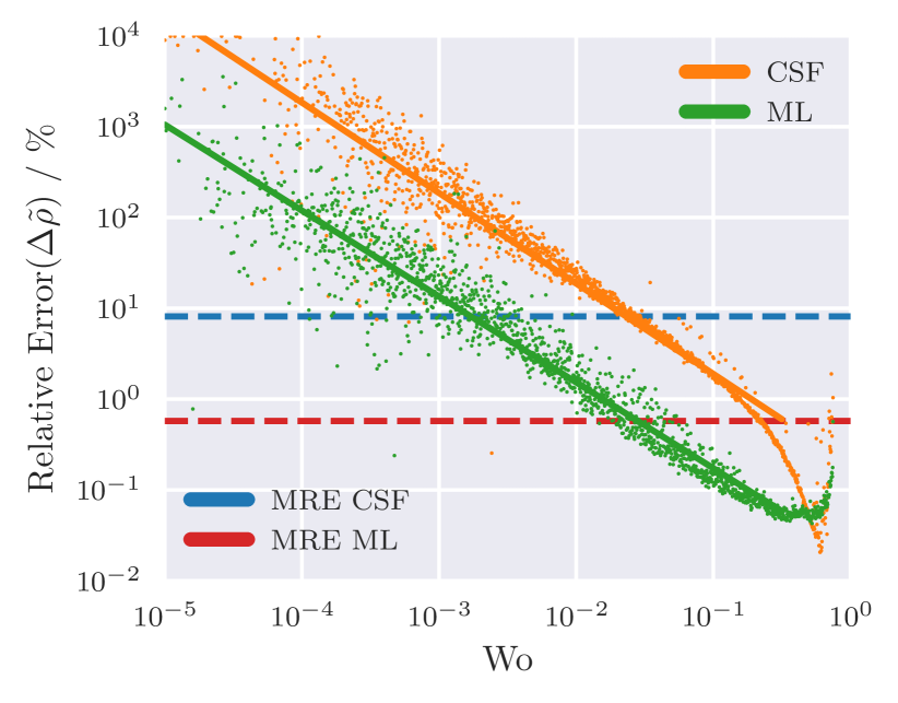
Figure 9: Scaling of the total mean relative error (MRE) of $\Delta\tilde{\rho}$ with the Worthington number (18).

Figure 8 also shows that the absolute errors in the parameter $\Delta\tilde{\rho}$ are generally larger because the shape is less sensitive to changes in $\Delta\tilde{\rho}$. A uniform absolute error in $\Delta\tilde{\rho}$ will result in a relative error scaling as $\mathrm{MRE}_{\Delta\tilde{\rho}}\sim\Delta\tilde{\rho}^{-1}$. Deviations from this scaling point to particularly sensitive or insensitive shapes. In Ref. 16, it has been proposed on a purely phenomenological basis that the relative error in the fitting accuracy of $\gamma$, which is proportional to the relative error in $\Delta\tilde{\rho}$, is best described by a parameter $\mathrm{Wo}$ (Worthington number), which is proportional to $\Delta\tilde{\rho}$,

$$\mathrm{Wo}\equiv\Delta\tilde{\rho}\frac{\tilde{V}}{\pi}=\frac{\Delta\rho gV}{\pi\gamma a}\,.$$ (18)

This parameter measures the distance to the detachment volume according to Tate’s law (17) such that $\mathrm{Wo}<1$ is bounded and $\mathrm{Wo}\simeq 1$ corresponds to a droplet close to detachment, while $\mathrm{Wo}\ll 1$ corresponds to droplets far from detachment. For a uniform absolute error in $\Delta\tilde{\rho}$, we thus expect a scaling $\mathrm{MRE}_{\Delta\tilde{\rho}}\sim\mathrm{Wo}^{-1}$. The scaling of the relative error $\mathrm{MRE}_{\Delta\tilde{\rho}}$ for CSF and ML approach is shown in Fig. 8. We find a power law scaling $\mathrm{MRE}_{\Delta\tilde{\rho}}=a\mathrm{Wo}^{\nu}$ and a fit in the linear region of the loglog plot in Fig. 8 gives the relative error scaling exponent and the scaling factor for CSF and ML,

$$\nu_{\text{CSF}} =-1.00~{},~{}\nu_{\text{ML}}=-0.95$$

$$a_{\text{CSF}} =-0.72~{},~{}a_{\text{ML}}=-1.71,$$ (19)

i.e., the exponent $\nu$ is indeed close to unity.

There is, however, the region of high Wo numbers $\mathrm{Wo}>0.1$, where CSF performs significantly better. Focusing on this region, Berry et al. found an exponent $\nu_{\text{CSF}}\approx-2$ indicating exceptionally small relative errors. Based on the shape diagram Fig. 5 we can actually rationalize this finding and provide a theoretical basis for the use of the Worthington number $\mathrm{Wo}$ as quality indicator in CSF. Close to a bifurcation such as the bifurcation $1\to 1,2,3$, where shapes $\Omega=2,3$ appear (at the yellow lines), shapes are most susceptible for parameter changes. This is evidenced, for example, by the vertical tangent in the $\tilde{V}(\tilde{p}_{\mathrm{L}})$ relation in Fig. 6 at this bifurcation. Similarly, there is a vertical tangent in the $\tilde{V}(\Delta\tilde{\rho})$ relation. Therefore, we expect exceptional shape sensitivity and, thus, a very well-conditioned shape fitting problem in the vicinity of this bifurcation. We already pointed out that this bifurcation happens almost at the same volume as detachment for $\Delta\tilde{\rho}\lesssim 1$, see shape diagram Fig. 5. Therefore, a parameter $\mathrm{Wo}\lesssim 1$ corresponds to a regime close to the detachment volume and, thus, close to the bifurcation where shapes $\Omega=2,3$ appear and, therefore, to the regime of a very well-conditioned shape fitting problem (at least for $\Delta\tilde{\rho}\lesssim 1$). Obviously, CSF works very well in exactly such well-conditioned parameter regions. This rationalizes the use of the Worthington number as quality indicator in CSF. Interestingly, the critical points at the tip of the shaded “triangles” enclosed by the yellow and blue bifurcation lines in the shape diagram Fig. 5, always lie at $\mathrm{Wo}=1/2$ according to the bifurcation condition (14) and $\tilde{p}_{\mathrm{cap}}=2$. Therefore, all shapes above the blue dashed line containing the critical points in the shape diagram Fig. 5 in the $\Delta\tilde{\rho}$-$\tilde{V}$ parameter plane have high Wo numbers $\mathrm{Wo}\geq 1/2$. CSF should work very well and give the best results in this region of the shape diagram. Figure 8 shows that only in this region CSF can outperform the ML approach.

ML gives a uniform absolute error over the full range of Wo numbers resulting in an exponent $\nu_{\text{ML}}\approx-1$. Therefore, the Worthington number Wo is less indicative for the performance of the ML approach, at least with the present set of training shapes uniformly distributed in the $\tilde{p}_{\mathrm{L}}$-$\Delta\tilde{\rho}$ plane. For smaller Wo numbers, ML gives on average a full order of magnitude more accurate estimates than CSF, while being four orders of magnitude faster.

VI.2 Adapting the training of the network

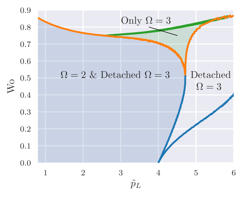
Figure 10: The training data sampling can be adjusted to be uniform in the $\tilde{p}_{\mathrm{L}}-\mathrm{Wo}$ plane. In the blue area only shapes of class 2 are sampled. In the green area only shapes of class 3 are sampled. We use the detachment condition discussed above to limit the sampling for class 3 shapes to pre-detachment shapes only.

Finally, we want to try to improve the ML approach such that it can handle all class 2 and 3 shapes while outperforming CSF for all Wo numbers. We can improve the performance of the ML approach selectively in the regions of high Wo numbers by adapting our training set such that it contains more shapes in this region. Sampling the training set uniformly from the shaded “triangle” enclosed by the yellow and blue bifurcation lines in the shape diagram Fig. 4 in the $\tilde{p}_{\mathrm{L}}$-$\Delta\tilde{\rho}$ plane leads to a training set biased towards small Wo numbers. Therefore, we adapt our training set such that it samples uniformly in the $\tilde{p}_{\mathrm{L}}$-$\mathrm{Wo}$ plane depicted in Fig. 10. In the new training set we include all class 3 shapes up to detachment (green sampling region in Fig. 10) as well as all class 2 shapes (blue sampling region in Fig. 10).

Generating a set of shapes sampled uniformly in the $\tilde{p}_{\mathrm{L}}$-$\mathrm{Wo}$ plane poses a problem, since the relationship between the control parameters of the simulation $\tilde{p}_{\mathrm{L}}$ and $\Delta\tilde{\rho}$ and the sampling parameter $\mathrm{Wo}$ is not known analytically. From data analysis we can extract a phenomenological dependency between $\Delta\tilde{\rho}$, the sampling parameters $\mathrm{Wo}$ and $\tilde{p}_{\mathrm{L}}$:

$$\Delta\tilde{\rho}\left(\tilde{p}_{\mathrm{L}},\mathrm{Wo}\right)\approx\frac{\pi}{43}\mathrm{Wo}^{0.91}\tilde{p}_{\mathrm{L}}^{\pi\left(1-\frac{\mathrm{Wo}}{4}\right)}\,.$$ (20)

This relation is based on an Ansatz $\Delta\tilde{\rho}\sim\mathrm{Wo}^{1-\epsilon}\tilde{p}_{\mathrm{L}}^{\delta}$ motivated by the definition of the Worthington number (18), $\Delta\tilde{\rho}\sim\mathrm{Wo}\tilde{V}^{-1}$ and an Ansatz $\tilde{V}\sim\tilde{p}_{\mathrm{L}}^{-\delta}$ for the pressure-volume relationship. While (20) provides a good mapping for $\tilde{p}_{\mathrm{L}}<3$ it lacks in accuracy for higher $\tilde{p}_{\mathrm{L}}$, where it can not be used for the generation of an evenly sampled training data set.

We ultimately generate the training set by the following algorithm, which does not use the relation (20). First, we pick $\mathrm{Wo}$ and $\tilde{p}_{\mathrm{L}}$ from a uniform distribution. Second, we algorithmically search for the upper and lower boundary of the shape diagram for $\Omega=2$ at the picked $\tilde{p}_{\mathrm{L}}$. Third, we numerically calculate the upper boundary shape and from it the upper boundary $\mathrm{Wo}^{\Omega=2}_{\mathrm{max}}$. If the picked $\mathrm{Wo}$ is bigger than $\mathrm{Wo}^{\Omega=2}_{\mathrm{max}}$ we search for a solution with $\Omega=3$. Should the picked $\mathrm{Wo}$ be smaller than $\mathrm{Wo}^{\Omega=2}_{\mathrm{max}}$ we search for a solution with $\Omega=2$. Last, the search for the target $\mathrm{Wo}$ is achieved by bisecting the interval between the upper and lower boundary of the corresponding valid parts of the shape diagram Fig. 4 in the $\tilde{p}_{\mathrm{L}}$-$\Delta\tilde{\rho}$ plane and determining the corresponding value of $\mathrm{Wo}$ till a numerically defined precision for $\mathrm{Wo}$ is reached.

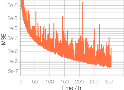
Figure 11: Training process of the adapted network in the first 300 hours of training.

This algorithm provides an evenly sampled training data set in the $\tilde{p}_{\mathrm{L}}$-$\mathrm{Wo}$ plane, which we use to train a new neural network, for which the training process is shown in Fig. 11.

The new sampling produces shapes that have a longer total arclength $L$ on average, thus we also modify the input sample count of the neural network to be $d=512$ and we append the pre-processed volume of the shape to the input vector providing a new feature that could help reduce the complexity caused by the increased sample count. Other pre-processed features available from the raw shape data could also be provided to further increase accuracy while reducing the complexity of the network.

The resulting network performs well over the full range $\mathrm{Wo}\in[0,1]$ as can be seen in Fig. 12. The absolute error is decreasing as $\mathrm{Wo}$ increases and the network gets extremely accurate for $\mathrm{Wo}\sim 0.8$. While the previous network performs better for small $\mathrm{Wo}$, the adapted network is a full order of magnitude better than the previous network for $\mathrm{Wo}\sim 0.8$.

The new network can also accurately solve the inverse problem for class 3 solutions up to detachment. In a comparison between CSF and the newly trained neural network for class 3 solutions we can see that the accuracy advantage of the CSF for high $\mathrm{Wo}$ melts away by including class 3 solutions up to detachment. This has to do with the fact that shapes become extraordinarily sensitive at the bifurcation between shapes 2 and 3 but as the class 3 solutions approach the detachment condition their $\mathrm{Wo}$ gets larger while the shape gets increasingly insensitive because class 3 shapes move away from the bifurcation line while increasing $\mathrm{Wo}$ up to detachment.

The ML approach provides good accuracy for all input shapes and thus gives a more reliable predicted set of shape parameters. The shape parameters predicted by the ML approach may also be improved further by using them as an initial guess in a CSF algorithm if needed.

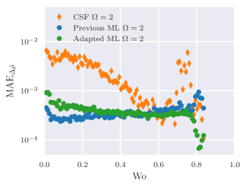
Figure 12: The absolute error of the adapted machine learning approach compared to the absolute error of the conventional shape fitting. Now class $2$ and $3$ solutions are used to train the network, however only class $2$ is shown. We omit all CSF fits with an absolute error that is higher then $10^{-1}$, while considering all ML predictions.

VI.3 Noise tolerance comparison

Comparing the ideal scenario of providing perfect input to both approaches might give an insight into the capabilities of both approaches in a best case scenario, it is, however, not realistic. Any given solution technique has to work with imperfect data in the real world. These imperfections might arise from a limited camera resolution, an imperfect edge detection software or by imperfections in the rest of the experimental setup. We want to discuss how both approaches can handle noisy input data. For this we apply a Gaussian blur to all shape coordinates $\vec{x}_{i}$ to transform them into a set of distorted shape coordinates $\vec{x}^{\prime}_{i}$. The Gaussian blur is centered around the origin so its mean is given by $\mu=0$ and the standard deviation $\sigma$ can be adjusted to create different noise amplitude scenarios.

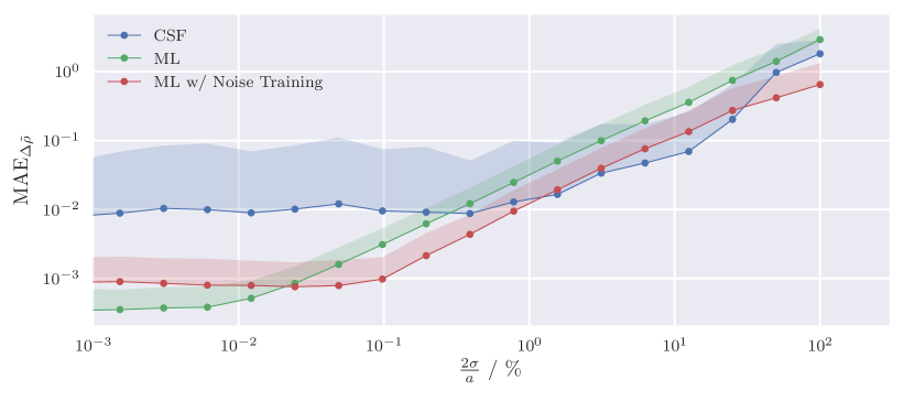
Figure 13: Comparison of the absolute error of class $2$ shapes with increasing Gaussian blur amplitudes added to the shape data. The shaded regions visualize the standard deviation of the mean absolute error. Because of the logarithmic scale only the upper bound is shown.

When comparing the performance of both methods in Fig. 13 we can observe that the ML approach that has been trained on undistorted data performs very well for low noise amplitude scenarios, but is outperformed by CSF for high noise amplitude scenarios. Again, we can adapt the training set to improve the ML approach. To increase the real world performance of the ML approach we can use noisy input data to train a new network that can handle noise better. We do this by training on a set of approximately $500,000$ shapes with a Gaussian blur applied to all shape coordinates, leading to a much improved noise resistance as can be seen in Fig. 13, while also maintaining almost equal precision in low noise amplitude scenarios. We also notice that changing from MSE to MAE as a training metric of the network improves the accuracy for noisy data even further, because then large individual errors do not dominate the overall mean error and the gradients in backpropagation are less noisy, leading to improved precision.

VII Discussion and conclusion

We introduced a novel ML approach to pendant drop tensiometry, where we train a deep neural network with numerically generated training shapes (solutions of the forward problem) for given pressure and interfacial tension in order to solve the backward problem of interfacial tension determination for a measured (or synthetically generated) droplet shape. We compare the performance of this mML approach to CSF approaches to tensiometry. The ML approach benefits from our ability to generate a arbitrarily large set of droplet training shapes numerically by solving the Young-Laplace equation (solving the forward problem) and control the distribution of training shapes in parameter space, which creates an ideal setting for supervised deep learning.

In order to rationalize the structure of shapes in parameter space we first discussed the physics of pendant drops and developed a simple classification of solution classes $\Omega=1,2,3,..$ by the number of bulges and necks. We obtained shape diagrams as a function of dimensionless apex pressure $\tilde{p}_{\mathrm{L}}$, dimensionless density difference $\Delta\tilde{\rho}$ (which is also a measure of capillary diameter), and volume $\tilde{V}$, i.e., shape diagrams in the $\tilde{p}_{\mathrm{L}}$-$\Delta\tilde{\rho}$ parameter plane under pressure control (Fig.  4) and in the $\Delta\tilde{\rho}$-$\tilde{V}$ parameter plane under volume control (Fig.  5). We identified the regions of existence of all shape classes and their bifurcations within the shape diagram. For pendant drops under volume control the shape sequence $\Omega=1\to 2\to 3$ is the sequence of energetically preferred states with shape $\Omega=2$ of a pendant drop with one bulge being the global energy minimum in a large volume range, i.e., everywhere where it exists. We also identified the detachment line of maximal volume within the shape diagrams and obtained the bifurcation condition (14), which also gives an excellent description of the detachment volume. Based on the shape diagrams we can propose several training strategies for supervised learning in the ML approach. We start with training shapes chosen uniformly in the $\tilde{p}_{\mathrm{L}}$-$\Delta\tilde{\rho}$ parameter plane.

The ML approach we provide is novel and performs well on this specific problem. It is not only more accurate than the tested conventional fitting scheme in large parts of the parameter space, but it is also orders of magnitude faster. Note that the precision of the inverse solution by CSF is bound by the precision target we provide and can outperform the precision of a neural network in the discussed “best case” fitting scenario in principle, but this will also take much longer. The hardware needed to execute a once trained neural network are miniscule in comparison to the hardware needed to perform numerical fitting of data sets in a reasonable time.

We chose a standard accuracy for the CSF approach and find that it outperforms the ML approach only in the regime of high Worthington numbers Wo close to unity. We can rationalize the use of the Worthington number as quality measure in conventional fitting approaches based on the shape diagrams by showing that high Wo numbers indicate a very well-conditioned shape fitting problem, where shapes are sensitive to parameter changes because they are closed to the shape bifurcation, where shapes $\Omega=2,3$ appear.

This is the motivation to adapt the training set for the ML approach further to contain shapes that are sampled with uniformly distributed Wo number. Using this strategy the ML approach’s precision for high Wo numbers is increased further.

This improvement by adaptation of the training set shows that there is certainly more potential for improvement in the ML approach either via the choice of training set or by further optimizing the network architecture which was a relatively simple five layer deep network (see Fig. 1). Recurrent neural networks (RNN) could also be tested to further improve performance and reliability, as well as convolutional neural networks for full image input analysis. These network types are generally more demanding on the hardware and could thus reduce the throughput of the network drastically. For rheological problems that consider a series of images - like a deflation experiment to determine the viscoelastic moduli - a long- short-term-memory (LSTM) input layer can be used to process the time component of the information in an efficient way to reduce the dimensionality of the data for the attached fully connected part of the network, as we will show in later work. Further improvement to the fully connected network type we provided can always be achieved by hyperparameter optimization and testing.

Because of the orders of magnitude faster computation time the ML approach can also be used for high-throughput analysis of droplet shapes in a short amount of time, or - provided a fast pre-processing algorithm - even real time video analysis in a dynamic experimental setting. Further investigations into the capabilities of neural networks in computationally taxing numerical fitting procedures, like pendant capsule elastometry [33, 28] or even viscoelastometry are the next step in future work, as the conventional fitting approach for those problems can be exponentially more demanding.

We make the deep neural network developed and trained within this work publicly available via GitHub [34] for further use in pendant drop tensiometry.

References

- Tate [1864] T. Tate, “On the magnitude of a drop of liquid formed under different circumstances,” Philos. Mag. 27, 176–180 (1864).
- Harkins and Brown [1919] W. D. Harkins and F. E. Brown, “The determination of surface tension (free surface energy), and the weight of falling drops: The surface tension of water and benzene by the capillary height method,” J. Am. Chem. Soc. 41, 499–524 (1919).
- Garandet, Vinet, and Gros [1994] J. P. Garandet, B. Vinet, and P. Gros, “Considerations on the pendant drop method: A new look at Tate’s law and Harkins’ correction factor,” J. Colloid Interface Sci. 165, 351–354 (1994).
- Yildirim, Xu, and Basaran [2005] O. E. Yildirim, Q. Xu, and O. A. Basaran, “Analysis of the drop weight method,” Phys. Fluids 17, 1–13 (2005).
- Fraser et al. [1971] M. E. Fraser, W. K. Lu, A. E. Hamielec, and R. Murarka, “Surface tension measurements on pure liquid iron and nickel by an oscillating drop technique,” Metall. Trans. 2, 817–823 (1971).
- Matsumoto et al. [2004] T. Matsumoto, H. Fujii, T. Ueda, M. Kamai, and K. Nogi, “Oscillating drop method using a falling droplet,” Rev. Sci. Instrum. 75, 1219–1221 (2004).
- Neeson, Chan, and Tabor [2014] M. J. Neeson, D. Y. C. Chan, and R. F. Tabor, “Compound Pendant Drop Tensiometry for Interfacial Tension Measurement at Zero Bond Number,” Langmuir 30, 15388–15391 (2014).
- Andreas, Hauser, and Tucker [1938] J. M. Andreas, E. A. Hauser, and W. B. Tucker, “Boundary tension by pendant drops,” J. Phys. Chem. 42, 1001–1019 (1938).
- Stauffer [1965] C. E. Stauffer, “The measurement of surface tension by the pendant drop technique,” J. Phys. Chem. 69, 1933–1938 (1965).
- Jůza [1997] J. Jůza, “The pendant drop method of surface tension measurement: Equation interpolating the shape factor tables for several selected planes,” Czechoslov. J. Phys. 47, 351–357 (1997).
- Hansen and Rødsrud [1991] F. K. Hansen and G. Rødsrud, “Surface tension by pendant drop. I. A fast standard instrument using computer image analysis,” J. Colloid Interface Sci. 141, 1–9 (1991).
- Song and Springer [1996] B. Song and J. Springer, “Determination of interfacial tension from the profile of a pendant drop using computer-aided image processing,” J. Colloid Interface Sci. 184, 64–76 (1996).
- Rıío and Neumann [1997] O. Rıío and A. Neumann, “Axisymmetric Drop Shape Analysis: Computational Methods for the Measurement of Interfacial Properties from the Shape and Dimensions of Pendant and Sessile Drops,” J. Colloid Interface Sci. 196, 136–147 (1997).
- Dingle et al. [2005] N. M. Dingle, K. Tjiptowidjojo, O. A. Basaran, and M. T. Harris, “A finite element based algorithm for determining interfacial tension () from pendant drop profiles,” J. Colloid Interface Sci. 286, 647–660 (2005).
- Hoorfar and W. Neumann [2006] M. Hoorfar and A. W. Neumann, “Recent progress in Axisymmetric Drop Shape Analysis (ADSA),” Adv. Colloid Interface Sci. 121, 25–49 (2006).
- Berry et al. [2015] J. D. Berry, M. J. Neeson, R. R. Dagastine, D. Y. C. Chan, and R. F. Tabor, “Measurement of surface and interfacial tension using pendant drop tensiometry,” J. Colloid Interface Sci. 454, 226–237 (2015).
- Touhami et al. [2011] Y. Touhami, G. H. Neale, V. Hornof, and H. Khalfalah, “Design and accuracy of pendant drop methods for surface tension measurement,” Colloids Surf. A 384, 442–452 (2011).
- [18] J. Hegemann and J. Kierfeld, “OpenCapsule: Pendant capsule elastometry,” .
- Pilozzi et al. [2018] L. Pilozzi, F. A. Farrelly, G. Marcucci, and C. Conti, “Machine learning inverse problem for topological photonics,” Commun. Phys. 1, 57 (2018).
- Kessler, El-Gizawy, and Smith [2007] B. S. Kessler, A. S. El-Gizawy, and D. E. Smith, “Incorporating Neural Network Material Models Within Finite Element Analysis for Rheological Behavior Prediction,” J. Press. Vessel Technol. 129, 58–65 (2007).
- DeVries, Thompson, and Meade [2017] P. M. DeVries, T. B. Thompson, and B. J. Meade, “Enabling large-scale viscoelastic calculations via neural network acceleration,” Geophys. Res. Lett. 44, 2662–2669 (2017).
- Saad, Policova, and Neumann [2011] S. M. Saad, Z. Policova, and A. W. Neumann, “Design and accuracy of pendant drop methods for surface tension measurement,” Colloids Surf. A 384, 442–452 (2011).
- Morita, Carastan, and Demarquette [2002] A. T. Morita, D. J. Carastan, and N. R. Demarquette, “Influence of drop volume on surface tension evaluated using the pendant drop method,” Colloid Polym. Sci. 280, 857–864 (2002).
- Padday, J. F. [1971] Padday, J. F., “Profiles of axially symmetric menisci,” Phil. Trans. Roy. Soc. Lond. A 269, 265–293 (1971).
- Maddocks [1987] J. H. Maddocks, “Stability and folds,” Arch. Ration. Mech. Anal. 99, 301–328 (1987).
- Eggers and Dupont [1994] J. Eggers and T. F. Dupont, “Drop Formation in a One-Dimensional Approximation of the Navier-Stokes Equation,” J. Fluid Mech. 262, 205–221 (1994).
- Gunde et al. [2001] R. Gunde, A. Kumar, S. Lehnert-Batar, R. Mäder, and E. J. Windhab, “Measurement of the surface and interfacial tension from maximum volume of a pendant drop,” J. Colloid Interface Sci. 244, 113–122 (2001).
- Hegemann et al. [2018] J. Hegemann, S. Knoche, S. Egger, M. Kott, S. Demand, A. Unverfehrt, H. Rehage, and J. Kierfeld, “Pendant capsule elastometry,” J. Colloid Interface Sci. 513, 549–565 (2018).
- Chollet et al. [2015] F. Chollet et al., “Keras,” https://keras.io (2015).
- Abadi et al. [2015] M. Abadi et al., “TensorFlow: Large-scale machine learning on heterogeneous systems,” (2015).
- Xu et al. [2015] B. Xu, N. Wang, T. Chen, and M. Li, “Empirical Evaluation of Rectified Activations in Convolutional Network,” CoRR (2015), arXiv:1505.00853 .
- Zeiler [2012] M. D. Zeiler, “ADADELTA: An Adaptive Learning Rate Method,” CoRR (2012), arXiv:1212.5701 .
- Knoche et al. [2013] S. Knoche, D. Vella, E. Aumaitre, P. Degen, H. Rehage, P. Cicuta, and J. Kierfeld, “Elastometry of Deflated Capsules: Elastic Moduli from Shape and Wrinkle Analysis,” Langmuir 29, 12463–12471 (2013).
- [34] F. Kratz and J. Kierfeld, “Pendant drop machine learning,” .