On the origin of the quantum group symmetry
in 3d quantum gravity

Abstract

It is well-known that quantum groups are relevant to describe the quantum regime of 3d gravity. They encode a deformation of the gauge symmetries parametrized by the value of the cosmological constant. They appear as a form of regularization either through the quantization of the Chern-Simons formulation or the state sum approach of Turaev-Viro. Such deformations are perplexing from a continuum and classical picture since the action is defined in terms of undeformed gauge invariance. We present here a novel way to derive from first principle and from the classical action such quantum group deformation. The argument relies on two main steps. First we perform a canonical transformation, which deformed the gauge invariance and the boundary symmetries, and makes them depend on the cosmological constant. Second we implement a discretization procedure relying on a truncation of the degrees of freedom from the continuum.

Introduction

When constructing a quantum theory, it is essential to identify the system’s relevant symmetries. Symmetries provide, thanks to Noether theorem [1], a non-perturbative handle which enables us to limit the quantization ambiguities, for example, by demanding that such symmetries are preserved upon quantization. They permit a powerful organization of the spectra by allowing the quantum states to form a representation of the symmetry group.

For gauge theories, such as gravity, it appears that this powerful tool is not available. Indeed, it is often believed that there are no symmetries in gravity, only gauge invariances. This leaves no means to use the power of having non-trivial conserved charges. Gauge invariances are conventionally understood [2] to be mere redundancies of the parametrization and, therefore, cannot help us to organize the quantum spectra. Physical states cannot be distinguished or labelled by the canonical generators associated with gauge invariance since by definition, these vanish on all physical states. We have a state of complete degeneracy, which is another expression of the celebrated problem of time [3], and this is the main reason behind the challenge of constructing a theory of quantum gravity.

Although there is no doubt that gauge invariance implies redundancy of the parametrization, there is a lingering sense that there is more to it [4]. After all, different formulations of gravity such as canonical formulation [5], metric formulation [6], tetrad formulation [7], teleparalell formulation [8] or shape-dynamics [9], possess different levels of redundancies and seem to present different advantages. Moreover, one seldom studies gravity in a fully gauge fixed form, such as [10, 11], which would be the most natural and beneficial option if redundancy was all there is to gauge invariance.

It is therefore natural to wonder whether there can be some other types of “hidden” symmetries that could be essential in the construction of the quantum theory, and whether such hidden symmetries could entertain a profitable relationship with the notion of gauge invariance? Critical examples of hidden symmetries in field theories are dualities [12], which are not manifest in the bulk Lagrangian. Other examples of hidden symmetries are dynamical symmetries [13] that arise in integrable systems.

One of the first and strongest indications that there are such “hidden” symmetries in gravity comes from the Turaev-Viro (TV) model [14], which is an expansion of the Ponzano-Regge [15] model. Indeed, in the presence of a cosmological constant, the quantum gravity partition function, can be constructed in terms of spin network states satisfying the intertwining properties of quantum groups [16, 17]. The TV model provides a discretization of the gravity path integral. This discretization satisfies two fundamental properties: First, each building block, given by the quantum group 6j symbol, is related in the limit of small Planck constant to the exponential of the classical gravity action [18]. Second, the partition function is invariant under refinement hence defines a continuum theory. The puzzle comes from the fact that there seem to be no sign of quantum group in the continuum theory, so that they seem to appear only after discretization and quantization.

Other mathematical justifications for quantum group symmetries in the context of 3d quantum gravity also originate from the fact that one can relate the TV model to the quantization of Chern-Simons (CS) [19, 20, 21, 22], and then prove that quantum groups appear in the definition of the quantum CS theory. For instance, the conjecture that quantum groups enter the construction of the CS partition function was first made by Witten [23] and proven by Reshetikhin-Turaev [24]. Another important evidence comes from the construction by Fock and Roskly [25] of a discrete version of the CS phase space, which includes from the get-go arbitrary sets of classical R-matrices. The quantization of this discrete phase, in terms of quantum groups, was achieved by Alekseev et al. [26, 27]. These approaches are top-down in the sense that quantum groups are postulated in the construction of partition functions or states or algebras and then justified by the consistency of their mathematical properties but not derived from first principles. In all these approaches, the R-matrix, which is the quantum group structure constant, is introduced by hand in the discretization and quantization processes.

There have also been many attempts to try to understand the appearance of quantum groups from a physical perspective. In [28], it was argued that quantum group deformation perturbatively appears in the limit of small cosmological constant. The works [29, 30] showed that the quantum group structure could appear in the regularization of the Hamiltonian constraint. In [31] a deformation of the Hamiltonian constraint, such that its kernel contains the TV amplitude, was found. We should also mention the seminal works [32, 33], where the quantum group symmetry is identified at the classical level for the Wess-Zumino model. While this is not the gravity context, the approach used there was an inspiration for our current work.

Despite all these attempts, no actual derivation of the TV model from a gravity action exists. Not to the level of satisfaction achieved for the Ponzano-Regge model where undeformed symmetry appears [34, 35, 36, 37]. All the justifications listed here point to the fact that the quantum group is the right symmetry to implement in the discrete and quantum regime, and that this symmetry somehow respects the dynamics of the theory. However, it is unclear what this symmetry exactly corresponds to. It cannot merely be gauge invariance since the Lorentz gauge group is independent of the cosmological constant. Also, it has to be appreciated that quantum groups introduce a preferred direction that selects a Cartan subalgebra from the onset. The source and nature of this preferred direction have been a long-standing puzzle.

The question we would like to address here is what is the classical origin of these quantum deformed symmetries, starting from the gravity action?

Answering this question relies on three concepts. The first key idea was first formulated in [38], further formalized in [39] and developed in [40, 41] at the quantum level. Concretely, these works establish that there are, actual symmetries in gravity represented by non-trivial canonical generators. These symmetries reveal themselves once we decompose a gravitational system into subsystems. Then the boundary of the subsystem decomposition supports the symmetry generators. The point is that these boundary symmetry generators are the relevant symmetry generators that one needs to use in order to construct the quantum theory. The quantum spacetime is then obtained as a fusion of quantum representations of the boundary symmetry group. This represents the quantum equivalent of the gluing of subregions. This idea is built upon the works of many who have demonstrated the central importance of boundary symmetry algebra in gravity [42, 43, 44, 45, 46, 47, 48] and developped the understanding of the nature of entanglement entropy in gauge theory [49, 50, 51, 52, 53, 54, 55].

The second and related idea, first proposed in [56], is that one can think of the process of discretizing a field theory, while respecting the bulk gauge invariance [36, 57] as a two-step process. The first step, that we just discussed, is the decomposition of the system into subregions and the second step is a coarse-graining operation where one replaces each cell of the decomposition by a vacuum solution of the bulk constraints. Consequently, the subregion boundaries, and their symmetry charges, encode all the relevant degrees of freedom of this corase grained data. This procedure leads to a discretization that respects, by construction, the fundamental invariance of the theory under study. It also leads to a new way to approach the continuum limit as a condensation of charge defects [58]. The choice of a solution on each cell corresponds to a vacuum choice at the quantum level [59]. This strategy has been developed in the case of three-dimensional gravity in [60, 61, 62].

The third concept is illustrated in the section II for 3d gravity and in [63] for 4d gravity. It uses the fact that it is possible to modify the expression of the boundary symmetries and their charges by the addition of boundary terms to the action. In the case of 3d gravity, the boundary symmetry is composed of the internal Lorentz symmetry and the translation symmetry. We show that it is necessary, in the presence of a non-vanishing cosmological constant, to add a boundary term to the action to ensure that the boundary translational symmetry is closed as an algebra. This boundary term, which implements a canonical transformation in the bulk, is the continuum analog of the classical R-matrix. It is given for 3d gravity by

$$\int_{\partial M}{\mathfrak{r}}_{ij}e^{i}\wedge e^{j},\qquad{\mathfrak{r}}_{ij}\equiv\epsilon_{ijk}n^{k},$$ (1)

where $n^{k}$ is a fiducial vector that is shown to be the quantum group preferred direction and whose norm square is proportional to the cosmological constant. We show that the presence of this boundary term affect the bulk connection and deforms the notion of gauge invariance, by replacing the usual gauge invariance by an equivalent one preserving the fiducial vector $n^{i}$. The fact that this is possible to introduce a fiducial vector without breaking, only deforming, gauge invariance is the central physical mechanism behind the appearance of quantum groups. It happens because the vector labels a bulk canonical transformation whose rotation can be rectified by a canonical boundary transformation. It is well-known that the charges of local rotations are given by the boundary coframe, that they form an algebra denoted $\mathfrak{su}$ and that the charges of local translations are given by the boundary connection [64]. After deformation we find that the translation generators form a subalgebra denoted $\mathfrak{an}$:

$$\{{P^{\prime}}_{\alpha},{P^{\prime}}_{\beta}\}={{P^{\prime}}}_{(\alpha\times\beta)\times n},\qquad{P}^{\prime}_{\phi}=\oint_{\partial\Sigma}\phi^{I}{\omega}_{I},$$ (2)

where $\times$ denote the cross product, $\Sigma$ is a 2d subregion and $\omega$ the (deformed) gravity connection. We also find that the cosmological constant enters, through $n$, in a deformation of the Lorentzian Gauss law. This gives us our first hint of the presence of a quantum group in the continuum theory.

In section III, we study the process of subdivision and coarse-graining as described previously. We show that after a choice of vacuum solution on each cell, the symplectic form of the continuum theory becomes finite-dimensional. It decomposes as a sum over the intersections of cells, these are the “links” of the decomposition.

For each link $\ell$ (and its dual $\ell^{*}$), we identify two holonomies $(H_{\ell},\tilde{H}_{\ell})$ belonging to the rotation group $\operatorname{SU}$ and two holonomies $(L_{\ell^{*}},\tilde{L}_{\ell^{*}})$ belonging to the group $\operatorname{AN}$ and we show that they form a ribbon structure:

$$\tilde{H}_{\ell}\tilde{L}_{\ell^{*}}={L}_{\ell^{*}}{H}_{\ell}.$$ (3)

The crux of the paper consists in proving that the phase space attached to each link is in fact the Heisenberg double ${\mathfrak{D}}$. As a manifold, the Heisenberg double is the cross-product group ${\mathfrak{D}}=\operatorname{SU}\bowtie\operatorname{AN}$ defined by the ribbon structure. The Poisson bracket we derived is compatible with the action of a Poisson-Lie group, which is the classical analog of the quantum group. The fact that classical analog of quantum group symmetries appears naturally when the phase space is a Heisenberg double has been established for a long time [65, 66, 67].

Note that in [68], a discrete model based on Heisenberg doubles attached to links was proposed. It was also argued there that it provides a discretization of 3d gravity with a non-zero cosmological constant, and later on, it was shown to lead to the Turaev-Viro amplitude upon quantization [31]. The relation with the classical continuum variables was missing. The derivation of this structure from the continuum action constitutes the main result of our work.

The article is organized as follow. Section I is essentially a review of existing material. We first recall the Hamiltonian analysis of 3d gravity with a non-zero cosmological constant. We emphasize that the rotational symmetry does not depend on the cosmological constant, so that it is not clear at first why a deformation of the symmetries should appear upon quantization.

In section II, we introduce the relevant boundary action which provides the right starting point for the discretization. We perform the Hamiltonian analysis of the action in these new variables. In particular, we obtain new rotational symmetries which do depend on the cosmological constant.

Section III provides the main result of the paper. We provide a detailed proof that the Heisenberg double phase space is obtained from our discretization. We highlight how the discretized variables we have obtained are related to the ones introduced in [68]. We show explicitly how the deformed symmetries of the Heisenberg double are recovered.

In Section IV, we recall how the quantum group structure appears from the quantization of the discrete variables we have constructed, following [31].

1 Canonical analysis of the 3d gravity action with a cosmological constant

We first recall the standard canonical analysis of the first order 3d gravity action with a non-zero cosmological constant. We consider a 3-dimensional manifold $M$ [69]. The greek indices $\alpha,\beta,..\in\{1,2,3\}$ are spacetime indices, while capital latin letters $I,J,..\in\{1,2,3\}$ are internal indices.

From metric formulation to first order formulation.

In the metric formulation the action is given by

$$S_{EH}[g_{\mu\nu}] =-\frac{1}{2\sigma\kappa}\int_{M}{d^{3}x\,\sqrt{\sigma\det(g_{\mu\nu})}\>\left(R[g_{\mu\nu}]-2\Lambda\right)},$$ (4)

where $\kappa={8\pi G}$ and $\sigma$ encodes the signature, $\sigma=-1$ for the Lorentzian case and $\sigma=+1$ for the Euclidean case. We introduce the frame field $e^{I}_{\mu}$, such that

$$g_{\mu\nu}=\eta_{IJ}e^{I}_{\mu}e^{J}_{\nu}\quad,\qquad e^{I}_{\mu}e^{\mu}_{J}=\delta^{I}_{J},\quad e^{I}_{\mu}e^{\nu}_{I}=\delta^{\nu}_{\mu}\,.$$ (5)

The internal metric is then $\eta=(+,+,\sigma)$. We also introduce the spin connection $\tilde{A}_{IJ}$, a $\mathfrak{so}(\eta)$ valued spin connection, such that $\tilde{A}^{IJ}=-\tilde{A}^{JI}$. The associated curvature is

$$R^{IJ}[\tilde{A}]=\text{d}\tilde{A}^{IJ}+\tilde{A}^{I}_{\>\>\,L}\wedge\tilde{A}^{LJ}.$$ (6)

Replacing these quantities in the action (4), we recover

$$S_{GR}[\tilde{A},e]=-\frac{1}{2\sigma\kappa}\int_{M}{\varepsilon_{IJK}\left(e^{I}\wedge R[\tilde{A}]^{JK}-\frac{\Lambda}{3}\,e^{I}\wedge e^{J}\wedge e^{K}\right)}\,.$$ (7)

It is common to rewrite the connection with a single index, using the Levi-Civita tensor, which also depends on the signature. Fixing $\epsilon_{123}=1$, we have $\epsilon^{123}=\sigma$ and furthermore

$$\epsilon^{\mu\nu\rho}\epsilon_{\mu\beta\gamma} =\sigma(\delta^{\nu}_{\beta}\delta^{\rho}_{\gamma}-\delta^{\rho}_{\beta}\delta^{\nu}_{\gamma})\,.$$ (8)

We have then

$$\tilde{A}^{J}=\frac{1}{2}\,\epsilon^{J}_{\>\>KL}\tilde{A}^{KL},\quad\tilde{A}^{JK}=\sigma\epsilon^{JK}{}_{I}\tilde{A}^{I}$$ (9)

$$R^{J}=\frac{1}{2}\,\epsilon^{J}_{\>\>KL}\,R^{KL},\quad R^{JK}=\sigma\epsilon^{JK}{}_{I}R^{I},\quad R^{I}=\mathrm{d}\tilde{A}^{I}-\frac{\sigma}{2}\epsilon^{I}{}_{JK}\tilde{A}^{J}\wedge\tilde{A}^{K}.$$ (10)

In order to have a curvature formula that does not depend on the signature, we can rescale the connection $A=-\sigma\tilde{A}$, so that

$$R^{I}[\tilde{A}]=-\sigma F^{I}[A]=-\sigma(\mathrm{d}A^{I}+{\frac{1}{2}}\epsilon^{I}{}_{JK}A^{J}\wedge A^{K}).$$ (11)

$A$ is still a $\mathfrak{so}(\eta)$ valued spin connection. Replacing this expression in the action, we obtain

$$S_{BF}[A,e] = \frac{1}{\kappa}\int_{M}{\left(\eta_{IJ}e^{I}\wedge F^{J}[A]+\sigma\frac{\Lambda}{6}\epsilon_{IJK}\,e^{I}\wedge e^{J}\wedge e^{K}\right)}$$ (12)

$$= \frac{1}{\kappa}\int_{M}\,e^{I}\wedge\left(F_{I}[A]+\sigma\frac{\Lambda}{3}\,E_{I}\right)\,,$$ (13)

where $E_{I}={\frac{1}{2}}\,(e\times e)_{I}$ is the area flux, $F_{I}[A]\equiv\text{d}A_{I}+{\frac{1}{2}}\,(A\times A)_{I}$ denotes the curvature of $A$ and $(A\times B)^{I}=\epsilon^{I}_{JK}A^{J}\wedge B^{K}$ denotes the cross-product of Lie algebra valued forms. In the following, we will work in units where $\kappa=1$, reestablishing the units when deemed useful.

Equations of motion.

One can couple this action to matter field via $S^{\mathrm{Mat}}(e,A;\phi)$ and we denote $\mathcal{P}_{I}\equiv-\frac{\delta S^{\mathrm{Mat}}}{\delta e^{I}}$ the energy momentum density and $\mathcal{J}^{I}\equiv-\frac{\delta S^{\mathrm{Mat}}}{\delta A_{I}}$ the angular-momentum density of the matter fields. The equations of motion are given by

$$F_{I}[A]+{\Lambda}\,\sigma E_{I}\approx\mathcal{P}_{I}\qquad\mathrm{d}_{A}e^{I}\approx\mathcal{J}^{I},$$ (14)

where $\mathrm{d}_{A}e^{I}\equiv\mathrm{d}e^{I}+(A\times e)^{I}$ is the torsion of $A$. In vaccuum, when no matter is present, the first equation is the curvature constraint $F_{\Lambda}^{I}\equiv F[A]^{I}+{\Lambda}\,E^{I}\approx 0$ and the second equation is the torsion free condition since $T^{I}\equiv{\mathrm{d}_{A}}e^{I}\approx 0$. We use the notation $\approx$ to stress that we have implemented the equations of motion.

Action symmetries

The action is invariant under a set of (gauge) symmetries. The first obvious symmetry is given by the $\mathfrak{so}(\eta)$ infinitesimal gauge transformations, parametrized by the scalar fields $\alpha^{J}$,

$$\delta_{\alpha}e^{I} = (e\times\alpha)^{I},\qquad\delta_{\alpha}A^{I}={\mathrm{d}_{A}}\alpha^{I},$$ (15)

$$\delta_{\alpha}\mathcal{J}^{I} = (\mathcal{J}\times\alpha)^{I},\qquad\delta_{\alpha}\mathcal{P}^{I}=(\mathcal{P}\times\alpha)^{I}.$$

They do not depend on the cosmological constant.
The second one is the ”shift” symmetry, parametrized by the scalar fields $\phi^{J}$,

$$\delta_{\phi}e^{I} = {\mathrm{d}_{A}}\phi^{I},\qquad\qquad\delta_{\phi}A^{I}=\Lambda\,(e\times\phi)^{I},$$ (16)

$$\delta_{\phi}\mathcal{J}^{I} = (\mathcal{P}\times\phi)^{I},\qquad\delta_{\phi}\mathcal{P}^{I}=\Lambda\,(\mathcal{J}\times\phi)^{I}.$$

These transformations are $\Lambda$ dependent. The last identity means that in the presence of a non-zero $\Lambda$, the notion of energy and momentum depends on the translational frame via the angular momenta density. In the same way that the notion of angular momenta depends on the rotational frame via the energy momentum density.
Diffeomorphism symmetry can be written, on-shell of the equations of motion, as a combined action of gauge and shift symmetries with field dependent parameters [70]. Given an infinitesimal diffeomorphism $\xi$, we define the field dependent parameters

$$\alpha_{\xi}^{I}=\iota_{\xi}A^{I},\quad\phi_{\xi}^{I}=\iota_{\xi}e^{I},$$ (17)

and we can express the action of an infinitesimal diffeomorphism as a gauge or shift symmetry on-shell.

$$\pounds_{\xi}A^{I} = \mathrm{d}\iota_{\xi}A^{I}+\iota_{\xi}\mathrm{d}A^{I}=\iota_{\xi}F^{I}_{\Lambda}+\delta_{\alpha_{\xi}}A^{I}+\delta_{\phi_{\xi}}A^{I}\approx\delta_{\alpha_{\xi}}A^{I}+\delta_{\phi_{\xi}}A^{I}$$ (18)

$$\pounds_{\xi}e^{I} = \mathrm{d}\iota_{\xi}e^{I}+\iota_{\xi}\mathrm{d}e^{I}=\iota_{\xi}T^{I}+\delta_{\alpha_{\xi}}e^{I}+\delta_{\phi_{\xi}}e^{I}\approx\delta_{\alpha_{\xi}}e^{I}+\delta_{\phi_{\xi}}e^{I}.$$ (19)

Symplectic form and Poisson brackets.

Let us now perform the Hamiltonian analysis of the action (12). We consider $M=\mathbb{R}\times\Sigma$. The symplectic potential associated with $S^{\text{BF}}_{M}$ is identify as the boundary variation $\delta S^{\text{BF}}_{M}\approx\Theta^{\text{BF}}_{\partial M}$. The symplectic form $\Omega^{\text{BF}}_{\Sigma}=\delta\Theta^{\text{BF}}_{\Sigma}$, associated with a Cauchy slice $\Sigma$ is

$$\Theta^{\text{BF}}_{\Sigma}=-\int_{\Sigma}\left\langle e\wedge\delta A\right\rangle,\quad\Omega^{\text{BF}}_{\Sigma}=-\int_{\Sigma}\left\langle\delta e\curlywedge\delta A\right\rangle,$$ (20)

where $\delta$ encodes the field variations, $\curlywedge$ is the extension of the wedge product to variational forms, and the pairing is given by $\left\langle\delta e\curlywedge\delta A\right\rangle=\eta_{IJ}\delta e^{I}\curlywedge\delta A^{J}$. Accordingly, the canonical variables are the pairs $(A^{I}_{a}(x),e_{b}^{J}(x))$ where $a,b$ are indices tangent to $\Sigma$, $a,b,..\in\{1,2\}$. The canonical Poisson bracket generated by (20) is simply, $\forall x,y\in\Sigma$,

$$\{A^{I}_{a}(x),e_{b}^{J}(y)\}=\kappa\,\epsilon_{ab}\,\eta^{IJ}\,\delta^{2}(x-y),\quad\{A^{I}_{a}(x),A_{b}^{J}(y)\}=0=\{e_{a}^{I}(x),e_{b}^{J}(y)\},$$ (22)

where we reinstated $\kappa$ for completeness.

Charges algebra

It is well-known that the total Hamiltonian and the generators of rotational and translational symmetry are given by boundary terms and satisfy a closed algebra. Let us recall that the Hamiltonian generator associated with a canonical field transformation $\delta_{\psi}$ is $H_{\psi}$ provided we have

$$\delta_{\psi}\lrcorner\,\Omega=\int_{\Sigma}(\left\langle\delta_{\psi}e\wedge\delta A\right\rangle-\left\langle\delta e\wedge\delta_{\psi}A\right\rangle)=-\delta H_{\psi}.$$ (23)

The Poisson bracket of two generators is defined to be

$$\{H_{\psi},H_{\psi^{\prime}}\}=\Omega(\delta_{\psi},\delta_{\psi^{\prime}})=\delta_{\psi}H_{\psi^{\prime}}.$$ (24)

In other words, the condition (23) means that the Hamiltonian generator $H_{\psi}$ generates the canonical transformation

$$\delta_{\psi}\cdot=\{H_{\psi},\cdot\}.$$ (25)

One denotes $J_{\alpha}$ the generator of rotational symmetry ($\delta_{\alpha}=\{J_{\alpha},\cdot\}$) , $P_{\phi}$ the generator of translational symmetry. They are given by

$$J_{\alpha} = \int_{\Sigma}\alpha_{I}(\mathcal{J}^{I}-\mathrm{d}_{A}e^{I})+\oint_{\partial\Sigma}\alpha_{I}e^{I},$$ (26)

$$P_{\phi} = \int_{\Sigma}\phi^{I}\left(\mathcal{P}_{I}-F_{I}(A)-\sigma\tfrac{\Lambda}{2}\,(e\times e)_{I}\right)+\oint_{\partial\Sigma}\phi^{I}A_{I},$$ (27)

The transformations associated to a parameter vanishing on the boundary are gauge transformations. Hence they have a vanishing charge. Their canonical generator vanishes on-shell since it is proportional to the constraints. On the other hand, transformations whose boundary parameters do not vanish, have non vanishing charges. They are the boundary symmetries. The corresponding boundary charges are given by

$$J_{\alpha}\approx\oint_{\partial\Sigma}\alpha_{I}e^{I},\qquad P_{\phi}\approx\oint_{\partial\Sigma}\phi^{I}A_{I}.$$ (28)

Using (24) and the expressions (15,16) for the transformations, one can evaluate the boundary charge algebra (reinstating $\kappa$)

$$\{J_{\alpha},J_{\beta}\}={\kappa}\,J_{(\alpha\times\beta)},\quad\{P_{\phi},P_{\psi}\}={\sigma}\,{\kappa}\,\Lambda\,J_{(\phi\times\psi)},$$

$$\{J_{\alpha},P_{\phi}\}={\kappa}\,P_{(\alpha\times\phi)}+{\kappa}\oint_{\partial\Sigma}\phi^{I}\mathrm{d}\alpha_{I}.$$ (29)

One sees that there exists a central extension in the commutator between $J_{\alpha}$ and $P_{\phi}$. Therefore this algebra is first class only for the transformation parameters $\alpha,\phi$ that are constant on $\partial\Sigma$. This set of constant parameters generate then global symmetry transformations which form a finite dimensional Poisson Lie algebra.

Quantum algebra of observables.

The corresponding quantum operators for the global charges are given by

$${\widehat{J}}^{I}\approx i\oint_{\partial\Sigma}\hat{e}^{I},\qquad{\widehat{P}}^{I}\approx i\oint_{\partial\Sigma}\hat{A}^{I}.$$ (30)

We require them to be be antihermitian ${\widehat{J}}^{\dagger}=-{\widehat{J}}$, ${\widehat{P}}^{\dagger}=-{\widehat{P}}$. They satisfy the Lie algebra brackets

$$[{\widehat{J}}_{I},{\widehat{J}}_{J}]=l_{P}\,\epsilon_{IJK}\,{\widehat{J}}^{K},\quad[{\widehat{J}}_{I},{\widehat{P}}_{J}]=l_{P}\,\epsilon_{IJK}\,{\widehat{P}}^{K},\quad[{\widehat{P}}_{I},{\widehat{P}}_{J}]=\sigma\,l_{P}\,\Lambda\,\epsilon_{IJK}\,{\widehat{J}}^{K},$$ (31)

with $l_{P}=\hbar{\kappa}$ the Planck length. The indices are raised with the metric $\eta_{IJ}$. Hence according to the signature $\sigma$ and the sign $s$ of the cosmological constant $\Lambda$, the quantum algebra of charges is isomorphic to a well-known Lie algebra ${\mathfrak{d}}_{\sigma s}$. We have ${\mathfrak{d}}_{++}=\mathfrak{so}(4)$ when dealing with a spherical space-time $S_{3}$, ${\mathfrak{d}}_{+-}={\mathfrak{sl}}(2,\mathbb{C})={\mathfrak{d}}_{-+}$ when dealing with a hyperbolical space-time $H_{3}$ or with a de Sitter space-time $dS_{3}$ and finally ${\mathfrak{d}}_{--}=\mathfrak{so}(2,2)$ when dealing with an anti de Sitter space-time $AdS_{3}$.

Gauge theory for ${\mathfrak{d}}_{\sigma s}$.

Let us note the generators of Lie algebra ${\mathfrak{d}}_{\sigma s}$ by ${{\bf J}}_{I}$ and ${{\bf P}}_{J}$, respectively the Lorentz/rotation generators and the boosts. To build the action, we introduce a pairing between the generators, i.e. an invariant bilinear form over ${\mathfrak{d}}_{\sigma s}$. The relevant one is ,

$$\left\langle{{\bf J}}_{I},{{\bf P}}_{J}\right\rangle=\eta_{IJ}=\left\langle{{\bf P}}_{I},{{\bf J}}_{J}\right\rangle,\quad\left\langle{{\bf J}}_{I},{{\bf J}}_{J}\right\rangle=0=\left\langle{{\bf P}}_{I},{{\bf P}}_{J}\right\rangle.$$ (32)

The frame field has value in the boosts, $e\equiv e^{I}{{\bf P}}_{I}$, whereas the connection has value in $\mathfrak{so}(\eta)$, $A\equiv A^{I}{{\bf J}}_{I}$. Hence, the curvature $F[A]$ is an object with value in $\mathfrak{so}(\eta)$, whereas the torsion $T[e,A]$ takes value in the boosts. In particular the covariant derivatives can be expressed in terms of the structure constant of $\mathfrak{so}(\eta)$.

$${\mathrm{d}_{A}}\alpha=\mathrm{d}\alpha+[A,\alpha],\quad\textrm{ with }\alpha=\alpha^{I}{{\bf J}}_{I},$$

$$\quad{\mathrm{d}_{A}}\phi=\mathrm{d}\phi+[A,\phi],\quad\textrm{ with }\phi=\phi^{I}{{\bf P}}_{I}.$$ (33)

We could now try to construct the LQG kinematical Hilbert space by imposing the Gauss constraint first as usually done. Since the rotational charge does not depend on $\Lambda$, we expect to recover after discretization the standard spin networks based on $\operatorname{SU}(2)$, just as when $\Lambda=0$. Hence the kinematical states are not given in terms of a quantum group structure. However we know that the quantum group structure needs to appear once we properly implement the dynamics. For example in the Turaev-Viro model [14], which gives the proper quantization of 3d gravity, the boundary states are given in terms of quantum group spin networks. This raises a fundamental puzzle and shows that the choice of discretization scheme could be at odd with the dynamics of the theory. While both formulations (with group or quantum group spin networks) should agree in the continuum limit, it is not clear how to define the quantum theory with undeformed spin networks and then to achieve a proper continuum limit, while the Turaev-Viro model is well-defined and also known to be invariant under refinement therefore defining a continuum theory. Resolving this tension means that one needs to deal at the classical level with a different rotational charge, which should depend on $\Lambda$.

Note also that an essential step to construct the quantum states is to discretize the theory, and in particular the charge information. We note that the translational charge algebra (29) does not form a closed algebra, rendering its discretization more obscure. As we will show modifying the rotational charge in a $\Lambda$ dependent way allows to perform the discretization without breaking the symmetry.

2 New variables and new action

In order to change the rotational charge structure, which should also depend on $\Lambda$, it is natural to add a boundary term.

2.1 Gravity Action and canonical transformation

Boundary term and canonical transformation.

Let us consider a general vector $n^{I}$ parametrizing the boundary contribution. We will see what further conditions $n$ is required to satisfy along the way. We consider then the original action (12) modified by the boundary term

$${S}_{QG}[e,A] \equiv S_{BF}[e,A]+\frac{1}{2{\kappa}}\int_{\partial M}\,{\mathfrak{r}}_{IJ}\,e^{I}\wedge e^{J}$$

$$= S_{BF}[e,A]+\frac{1}{2{\kappa}}\int_{\partial M}(e\times e)_{I}n^{I}$$

$$= \frac{1}{{\kappa}}\int_{M}\,e^{I}\wedge\left(F_{I}[A]+\sigma\frac{\Lambda}{6}\,\epsilon_{IJK}\,e^{J}\wedge e^{K}\right)+\frac{1}{2{\kappa}}\int_{M}\mathrm{d}\left((e\times e)_{I}n^{I}\right).$$ (35)

The boundary term does not modify the equations of motion. We note that while $n$ is defined first on the boundary $\partial M$, it can be naturally extended to the bulk $M$ using Stokes theorem. As before we will work with ${\kappa}=1$ until deemed necessary.

To perform the Hamiltonian analysis of the new action, we assume as before that $M=\mathbb{R}\times\Sigma$. The new symplectic potential is

$$\Theta_{QG}=\int_{\Sigma}e_{I}\wedge\delta A^{I}-\frac{1}{2}\delta\int_{\Sigma}(e\times e)_{I}n^{I}=\int_{\Sigma}e_{I}\wedge\delta\omega^{I}-{\frac{1}{2}}\int_{\Sigma}(e\times e)_{I}\cdot\delta n^{I},$$ (36)

where we have introduced a new connection

$$\omega^{I}\equiv A^{I}+(n\times e)^{I}.$$ (37)

We see from (36) that we have an extra pair of conjugated variables $(n,E={\frac{1}{2}}(e\times e))$ where the area flux $E$ is conjugated to $n$. We note that if $n$ is treated as a kinematical structure, it is required to be constant as a field, $\delta n=0$, and the boundary term simply induces a canonical transformation (in the bulk) that modifies the original symplectic potential (20). Note that this conditions forbids the vector $n^{I}$ to be related to the boundary normal.

This canonical transformation only modifies the connection. We will assume that $\delta n=0$ from now on. Hence $(e_{a}^{I},\omega_{b}^{J})$ is our new canonical pair, $\forall(x,y)\in\mathbb{R}^{2}$,

$$\{{\omega}^{I}_{a}(x),e_{b}^{J}(y)\}={\kappa}\,\epsilon_{ab}\,\eta^{IJ}\,\delta^{2}(x-y),\quad\{{\omega}^{I}_{a}(x),{\omega}_{b}^{J}(y)\}=0=\{e_{a}^{I}(x),e_{b}^{J}(y)\},$$ (38)

With such a change of variables, we can express the curvature in terms of the new connection $\omega$

$$F[A]=F[\omega+e\times n]=F[\omega]+\mathrm{d}_{\omega}(e\times n)+{\frac{1}{2}}(e\times n)\times(e\times n),$$ (39)

where $\mathrm{d}_{\omega}\alpha=\mathrm{d}\alpha+\omega\times\alpha$. To evaluate the action in terms of $\omega$, one establishes that

$${\frac{1}{2}}e\cdot((e\times n)\times(e\times n))=\frac{\sigma n^{2}}{6}e\cdot(e\times e).$$ (41)

We choose the normalization $n^{2}=-\Lambda$, as a new restriction on $n$, so that the last term of (39) compensates the term proportional to $\Lambda$ in the action (35).

With the assumptions that $\delta n=0,$ and $n^{2}=-\Lambda$, the change of variables implies that the action (35) becomes

$${S}_{QG}=\int_{M}\,\left(e\cdot F[A]+\sigma\frac{\Lambda}{3}\,e\cdot E\right)+\int_{\partial M}E\cdot n = \int_{M}\,\left(e\cdot F[\omega]-E\cdot\mathrm{d}_{\omega}n\right).$$ (42)

While the original action (35) couples the frame $e$ and flux $E=\tfrac{1}{2}(e\times e)$ the modified action is achieving a “separation of variables” where $e$ and $E$ are decoupled. This will simplify the analysis of the theory and its symmetries.

The equations of motion of the new action (42) are now

$$F_{I}[\omega]-(e\times\mathrm{d}_{\omega}n)_{I}\approx\mathcal{P}^{\prime}_{I}\qquad\mathrm{and}\qquad \mathrm{d}_{\omega}e^{I}+\frac{1}{2}[(e\times e)\times n]^{I}\approx\mathcal{J}^{\prime I}.$$ (43)

The matter spin density $\mathcal{J}^{\prime}\equiv-\frac{\delta S_{\mathrm{QG}}}{\delta\omega}$ is unchanged while the energy-momentum density $\mathcal{P}^{\prime}\equiv-\frac{\delta S_{\mathrm{QG}}}{\delta e}$ is redefined:

$${\mathcal{J}^{\prime}}_{I}=\mathcal{J}_{I},\qquad{\mathcal{P}^{\prime}}_{I}=\mathcal{P}_{I}+(n\times\mathcal{J})_{I}.$$ (44)

Nature of the vector $n$.

In the Euclidean case $\sigma=+1$, the normalization condition $n^{2}=-\Lambda$ can be achieved by a real vector in the hyperbolic case ($\Lambda<0$) or by a pure imaginary vector in the spherical case ($\Lambda>0$). If $\Lambda=0$, then either $n=0$ or it is specified by a Grassmanian number.

In the Lorentzian case, $n$ is time-like (or imaginary space-like) for the de Sitter case and space-like (or imaginary time-like) for the AdS case. When $\Lambda=0$ we have two options, $n$ is either a non trivial null vector or it simply vanishes.

	Euclidean	Lorentzian
Flat: $\Lambda=0$	$n=0$ or $n$ is Grassmanian	$n=0$ or $n$ is light-like
AdS:$\Lambda<0$	$n$ is space-like	$n$ is space-like or imaginary time-like
dS:$\Lambda>0$	$n$ is imaginary	$n$ is time-like or imaginary space-like

Symmetries of the action.

Since the action $S_{\textrm{QG}}$ depends explicitely on a vector $n$, one might worry that this vector acts as a background structure and that this action explicitly breaks local rotational symmetry. It turns out, quite remarkably, that this is not the case. The action is still invariant under gauge transformations generalizing the local $\mathrm{SO}(\eta)$ transformations (15) and the shift transformations (16).

First let us notice that since we required $n$ to be constant as a field $\delta n=0$ this implies that it will not change under the symmetry transformations, spanned by the Hamiltonain generators $H_{\psi}$ (with $\psi=\alpha,\phi$),

$$\delta_{\psi}n=\{H_{\psi},n\}=0.$$ (45)

As a consequence, $n$ can be seen as a scalar for the different gauge transformations. In the following, we are going to determine the shape of the gauge transformations on the field $e$ and $\omega$ which are consistent with this constraint $\delta_{\psi}n=0$. In order to distinguish the new infinitesimal transformations from the previous one, we will note them $\delta^{\prime}_{\psi}$. We demand therefore that $\delta^{\prime}_{\psi}n=0$, for $\psi=\alpha,\phi$.

Let us study the set of transformations, generalizing the $\mathfrak{so}(\eta)$ infinitesimal transformations, that we parametrize by $\alpha^{I}$. Since we have that

$$\delta_{\alpha}^{\prime}n^{I} = 0,$$ (46)

and that we still have that $e^{I}$ should transform as a vector,

$$\delta^{\prime}_{\alpha}e^{I} = (e\times\alpha)^{I}=\delta_{\alpha}e^{I}.$$ (47)

We can use the transformations of $A$ and the relation between $A$ and $\omega$ to infer the transformations of $\omega$.

$$\delta^{\prime}_{\alpha}A=\delta^{\prime}_{\alpha}({\omega}-n\times e)=\delta^{\prime}_{\alpha}{\omega}-n\times\delta^{\prime}_{\alpha}e\Leftrightarrow\delta^{\prime}_{\alpha}\omega^{I}=\mathrm{d}_{\omega}\alpha^{I}+(e\times(n\times\alpha))^{I}\equiv D\alpha^{I}.$$ (48)

The second set of transformations, parametrized by $\phi$ generalizes the shift symmetry. We still demand that $\delta^{\prime}_{\phi}n^{I}=0$. We have

$$\delta^{\prime}_{\phi}\omega^{I} = (\phi\times\mathrm{d}_{\omega}n)^{I}$$ (49)

$$\delta^{\prime}_{\phi}e^{I} = \mathrm{d}_{\omega}\phi^{I}+((e\times\phi)\times n)^{I}\equiv\tilde{D}\phi^{I}.$$ (50)

These transformations satisfy $\delta^{\prime}_{\phi}e^{I}=\delta_{\phi}e^{I}+\delta_{\alpha=\phi\times n}e^{I}$.

It is worth noticing that now both types of gauge transformations are dependent on the cosmological constant through the vector $n$ and both leave the auxiliary vector $n$ invariant. We emphasize again that this implies that the vector $n$ is a scalar for such gauge transformations.

2.2 Deformed boundary symmetry algebra and Manin pairs

New charges algebra.

One can wonder at this stage, what have we gained by going to this more elaborate description of the same physical system? The clear advantage of this description shows up when we look at the symmetry algebra and the transformations of the spin and energy momenta densities. These transformation can be deduced from (47,48,50) by acting on the LHS of the constraints (43). For instance one finds that

$$\delta^{\prime}_{\alpha}\mathcal{J}^{\prime}=\mathcal{J}^{\prime}\times\alpha,\qquad\delta^{\prime}_{\phi}\mathcal{P}^{\prime}=(\mathcal{P}^{\prime}\times\phi)\times n,$$ (51)

which shows that the modified energy-momentum density transforms homogeneously under a local translation, unlike (1). The charges associated with these transformations ${\delta}^{\prime}_{\alpha}\lrcorner\,\Omega=-\delta{J}^{\prime}_{\alpha}$ and $\delta^{\prime}_{\phi}\lrcorner\,\Omega=-\delta{P}^{\prime}_{\phi}$, are given by

$${J}^{\prime}_{\alpha} = \int_{\Sigma}\alpha_{I}\left[\mathcal{J}^{\prime}-\mathrm{d}_{\omega}e-\tfrac{1}{2}((e\times e)\times n)\right]^{I}+\oint_{\partial\Sigma}\alpha_{I}e^{I},$$ (52)

$${P}^{\prime}_{\phi} = \int_{\Sigma}\phi^{I}\left[\mathcal{P}^{\prime}-F[\omega]+(e\times\mathrm{d}_{\omega}n)\right]_{I}+\oint_{\partial\Sigma}\phi^{I}\omega_{I}.$$ (53)

On-shell, these charges are simply

$${J}^{\prime}_{\alpha}=\oint_{\partial\Sigma}\alpha_{I}e^{I}=J_{\alpha},\qquad{P}^{\prime}_{\phi}=\oint_{\partial\Sigma}\phi^{I}{\omega}_{I}=P_{\phi}+J_{\phi\times n}.$$ (54)

The charge algebra is such that $J^{\prime}_{\alpha}$ and $P^{\prime}_{\phi}$ generate two subalgebras given by

$$\{J^{\prime}_{\alpha},J^{\prime}_{\beta}\}={\kappa}\,J^{\prime}_{\alpha\times\beta}, \qquad\{{P^{\prime}}_{\phi},{P^{\prime}}_{\psi}\}={\kappa}\,{{P^{\prime}}}_{(\phi\times\psi)\times n}+{\kappa}\,\oint_{\partial\Sigma}(\phi\times\psi)\cdot\mathrm{d}n,$$ (55)

while the cross-commutator is given by

$$\{J^{\prime}_{\alpha},{P^{\prime}}_{\phi}\} = {\kappa}\,{P^{\prime}}_{\alpha\times\phi}+J^{\prime}_{\phi\times(\alpha\times n)}+{\kappa}\,\oint_{\partial\Sigma}\phi\cdot\mathrm{d}\alpha.$$ (56)

The proof is detailed in the appendix A.1. We emphasize that we are using the simple derivative $\mathrm{d}$ since $n$ is a scalar in terms of the gauge transformations.

We see that the commutator of energy-momentum charges possesses a central charge if $n$ is not constant. From now on, we assume that $\mathrm{d}n=0$. In this case, we see that the modified energy momentum charges ${P^{\prime}}_{\alpha}$ form a closed subalgebra and the central charge is concentrated of the bracket between rotation generators $J^{\prime}$ translation/boost generators ${P^{\prime}}$. This is in sharp contrast with the original description (29), where the momentum generators do not form a closed subalgebra and it is the main reason behind the canonical transformation and the normalisation $n^{2}=-\Lambda$.

Another condition on $n$.

Before discussing the shape of the global symmetries, it will be useful to fix for once and for all the vector $n$. Without loss of generality, we can always choose the vector $n$ as defining the direction $3$, $n^{I}=(0,0,n^{3})$. As we have seen earlier in (42), according to the normalization condition $n^{2}=-\Lambda$, the vector $n$ can be space-like or time-like, or even imaginary. Since we have fixed the direction of $n$, this means that the metric should also depend on $s$, the sign of $\Lambda$. Let us review the different cases.

If we are in the Euclidean case with $\Lambda>0$, then $n^{I}=(0,0,i\sqrt{\Lambda})$ and the Euclidean metric is consistent. In the other cases where $\Lambda\neq 0$, we will take $n^{I}=(0,0,-s\sigma\sqrt{|\Lambda|})$ and a metric $\eta^{\sigma s}$ such that

$$\eta^{\sigma s}_{IJ}=\mathrm{diag}(+,-s\sigma,-s),\quad n^{I}\eta_{IJ}n^{J}=-\,s\,|\Lambda|=-\,\Lambda.$$ (57)

Finally, in the case where $\Lambda=0$, we stick to the usual metric $\eta_{IJ}=\mathrm{diag}(+,+,\sigma)$. Fixing such convention will allow to connect more easily to the usual quantum group formalism where it is always the third direction that is picked out as preferred. Let us review the full set of constraints we have on $n$,

$$\delta n=0\,\,(\Rightarrow\delta^{\prime}_{\alpha}n=\delta^{\prime}_{\phi}n=0),\quad n^{2}=-\Lambda,\quad\mathrm{d}n=0,\quad n^{I}=(0,0,n^{3}).$$ (58)

While the symmetry structure of the metric is still isomorphic to $\mathfrak{so}(\eta)$, the time direction is not always the same in the Lorentzian case, to account for $n$ being space-like or time-like. Let us review the different explicit forms of $\mathfrak{so}(\eta)$. We note ${{\bf J}}^{I}$ their generators. The commutation relations are simply $[{{\bf J}}^{I},{{\bf J}}^{J}]=\epsilon^{IJ}{}_{K}{{\bf J}}^{K}$, where we use the the metric $\eta_{\sigma s}$ to lower the index $K$. This means that we have different algebras for different choices of $(\sigma,s)$. We denote the different cases by $\mathfrak{su}_{\sigma s}$

$$\mathfrak{su}_{+-}=\mathfrak{su}(2): [{{\bf J}}_{1},{{\bf J}}_{2}]={{\bf J}}_{3},\quad[{{\bf J}}_{2},{{\bf J}}_{3}]={{\bf J}}_{1},\quad[{{\bf J}}_{3},{{\bf J}}_{1}]={{\bf J}}_{2},$$

$$\mathfrak{su}_{-+}=\mathfrak{su}(1,1): [{{\bf J}}_{1},{{\bf J}}_{2}]=-{{\bf J}}_{3},\quad[{{\bf J}}_{2},{{\bf J}}_{3}]={{\bf J}}_{1},\quad[{{\bf J}}_{3},{{\bf J}}_{1}]={{\bf J}}_{2}$$

$$\mathfrak{su}_{--}={\mathfrak{sl}}(2,\mathbb{R}): [{{\bf J}}_{1},{{\bf J}}_{2}]={{\bf J}}_{3},\quad[{{\bf J}}_{2},{{\bf J}}_{3}]={{\bf J}}_{1},\quad[{{\bf J}}_{3},{{\bf J}}_{1}]=-{{\bf J}}_{2}.$$ (59)

Quantum algebra of observables.

The algebra given in (55) and (56) is first class only for the transformation parameters that are constant on the boundary. Such a set of constant parameters generates then global symmetry transformations which form a finite dimensional Poisson Lie algebra. The associated quantum algebra is now generated by the quantisation of the global charges

$${\widehat{J}}^{\prime I}={\widehat{J}}^{I}=i\oint\hat{e}^{I},\qquad{\widehat{P}}^{\prime}_{I}=i\oint\hat{{\omega}}_{I}.$$ (60)

As we have seen in (54), we have just performed a linear change of basis, hence the global charges still form an algebra isomorphic to ${\mathfrak{d}}_{\sigma s}$, with ${\mathfrak{d}}_{++}=\mathfrak{so}(4)\sim\mathfrak{su}(2)\oplus\mathfrak{su}(2),\,{\mathfrak{d}}_{+-}={\mathfrak{sl}}(2,\mathbb{C})={\mathfrak{d}}_{-+},$ and ${\mathfrak{d}}_{--}=\mathfrak{so}(2,2)\sim{\mathfrak{sl}}(2,\mathbb{R})\oplus{\mathfrak{sl}}(2,\mathbb{R}).$ The physical reality condition that arises from the quantisation of the global algebra with $e,{\omega}$ real (60) demands that all generators are antihermitian and that the vector $n$ is real:

$${\widehat{J}}^{\prime\dagger}=-{\widehat{J}}^{\prime},\quad{\widehat{P}}^{\prime\dagger}=-{\widehat{P}}^{\prime},\quad\bar{n}=n.$$ (61)

We note that the Euclidean case with positive cosmological constant does not have a real $n$, hence we will not discuss it here. It requires a more careful analysis on the reality condition.

${\mathfrak{d}}_{\sigma s}$ as a Manin pair.

The Lie algebra ${\mathfrak{d}}_{\sigma s}$ has the structure of a Manin triple, that is, it is a classical Drinfeld double that can be written as a matching pair ${\mathfrak{d}}_{\sigma s}={\mathfrak{g}}\bowtie{\mathfrak{g}}^{*}$ [16]. By construction, ${\mathfrak{d}}_{\sigma s}$ possesses an invariant symmetric pairing denoted $\left\langle\cdot,\cdot\right\rangle$ of signature $(3,3)$ and it can be decomposed as a pair of isotropic algebras

$${\mathfrak{d}}={\mathfrak{g}}\oplus{\mathfrak{g}}^{*},\qquad\left\langle\cdot,\cdot\right\rangle|_{{\mathfrak{g}}}=0=\left\langle\cdot,\cdot\right\rangle|_{{\mathfrak{g}}^{*}}.$$ (62)

The symmetric pairing is simply the canonical pairing between ${\mathfrak{g}}$ and ${\mathfrak{g}}^{*}$. Given ${\mathfrak{d}}_{\sigma s}$, its subalgebra ${\mathfrak{g}}$ is the subalgebra $\mathfrak{su}_{\sigma s}$ with generators ${{\bf J}}^{I}$ satisfying the algebra (2.2)

$$[{{\bf J}}^{I},{{\bf J}}^{J}]=\epsilon^{IJ}{}_{K}{{\bf J}}^{K}.$$ (63)

The dual algebra ${\mathfrak{g}}^{*}$ is the algebra with generators

$$\tau_{I}\equiv{{\bf P}}_{I}+n^{J}\epsilon_{IJK}{{\bf J}}^{K}={{\bf P}}_{I}+(n\times{{\bf J}})_{I}$$ (64)

which satisfy the $\mathfrak{an}$ algebra commutation relations

$$[\tau_{I},\tau_{J}]=C_{IJ}{}^{K}\tau_{K}\quad\textrm{with }\quad C_{IJ}{}^{K}=\sigma(n_{I}\delta_{J}^{K}-n_{J}\delta_{I}^{K}).$$ (65)

With our specific choice $n^{I}=(0,0,s\sigma\sqrt{|\Lambda|})$ and $\eta_{IJ}=\mathrm{diag}(+,-s\sigma,-s)$, we get an algebra which is independent of $\sigma$ and $s$: the Lie algebra $\mathfrak{an}$ given by

$$[\tau_{1},\tau_{2}]=0,\qquad[\tau_{3},\tau_{1}]=\sqrt{|\Lambda|}\tau_{1},\qquad[\tau_{3},\tau_{2}]=\sqrt{|\Lambda|}\tau_{2}.$$ (66)

The symmetric pairing is simply

$$\left\langle\tau_{J},{{\bf J}}^{I}\right\rangle=\delta^{I}_{J}=\left\langle{{\bf J}}^{I},\tau_{J}\right\rangle,\qquad\left\langle{{\bf J}}^{I},{{\bf J}}^{J}\right\rangle=0=\left\langle\tau_{I},\tau_{J}\right\rangle.$$ (67)

We emphasize that the structure constant $C_{IJK}$ is not cyclic as $\epsilon^{IJK}$. The last structure constant is the mixed one

$$[{{\bf J}}^{I},\tau_{J}]=C_{JK}{}^{I}{{\bf J}}^{K}+\epsilon^{I}{}_{J}{}^{K}\tau_{K},$$ (68)

which is uniquely determined from (63,65) by the Killing form defining property $\left\langle[X,Y],Z\right\rangle=\left\langle X,[Y,Z]\right\rangle.$

The Drinfeld double decomposition of ${\mathfrak{d}}_{\sigma s}$ is given by the Iwasawa decomposition

$${\mathfrak{d}}_{\sigma s}=\mathfrak{su}_{\sigma s}\bowtie\mathfrak{an}\sim\mathfrak{an}\bowtie\mathfrak{su}_{\sigma s}.$$ (69)

Such an Iwasawa decomposition does not exist for ${\mathfrak{d}}_{++}\sim\mathfrak{so}(4)$, which is why we do not consider it. The cross commutator (68) includes an action of $\mathfrak{su}_{\sigma s}$ on $\mathfrak{an}$ of and retro-action of $\mathfrak{an}$ on $\mathfrak{su}_{\sigma s}$. We can isolate the different actions, by considering the projection of the cross commutator [72].

$${{\bf J}}^{I}\rhd\tau_{J}\equiv[{{\bf J}}^{I},\tau_{J}]_{{\mathfrak{an}}} =\epsilon^{I}{}_{J}{}^{K}\tau_{K},\quad {{\bf J}}^{I}\lhd\tau_{J}\equiv[{{\bf J}}^{I},\tau_{J}]_{{\mathfrak{su}}}=C_{JK}{}^{I}{{\bf J}}^{K}$$ (70)

$$\tau_{J}\lhd{{\bf J}}^{I}\equiv[\tau_{J},{{\bf J}}^{I}]_{{\mathfrak{an}}} =-{{\bf J}}^{I}\rhd\tau_{J},\quad \tau_{J}\rhd{{\bf J}}^{I}\equiv[\tau_{J},{{\bf J}}^{I}]_{{\mathfrak{su}}}=-{{\bf J}}^{I}\lhd\tau_{J}.$$ (71)

The relations (63), (65) and (68) are the counterparts of (31). They are the defining relations of ${\mathfrak{d}}_{\sigma s}$ as a Drinfeld double of $\mathfrak{su}$ (with a non-trivial cocycle) [16]. Again, we emphasize that with the convention we took, the $\mathfrak{an}$ sector always singles out the direction 3 and is independent of $(\sigma,s)$. As we will see later, the function algebra over the Lie group $\operatorname{AN}$ is isomorphic to the enveloping algebra ${{\mathcal{U}}_{q}(\mathfrak{su}(2))}$ which is always defined with the preferred direction 3. Given $\alpha,\beta\in\mathfrak{su}$ and $\phi,\psi\in\mathfrak{an}$ we can summarize the Drinfeld double algebra as [72]

$$[\alpha,\beta]=(\alpha\times\beta)_{I}{{\bf J}}^{I},\qquad[\phi,\psi]=((\phi\times\psi)\times n)^{I}\tau_{I}$$ (72)

$$\alpha\rhd\phi=(\alpha\times\phi)^{I}\tau_{I}=-\phi\lhd\alpha,\quad\alpha\lhd\phi=(\phi\times(\alpha\times n))_{I}{{\bf J}}^{I}=-\phi\rhd\alpha.$$ (73)

and the cross-commutator is

$$[\alpha,\phi]=\alpha\rhd\phi+\alpha\lhd\phi=-\phi\lhd\alpha-\phi\rhd\alpha,$$ (74)

in accordance with (70), (71) and (56).

Role of the matrix ${\mathfrak{r}}$.

As we have seen, the source of the deformation of the boundary symmetry algebra is contained in the “little” r-matrix ${\mathfrak{r}}_{IJ}=\epsilon_{IJK}n^{K}$ that sources the canonical transformation.

Let us clarify the algebraic role of ${\mathfrak{r}}$. This r-matrix can be seen as building up the $\mathfrak{an}$ Lie algebra structure from the $\mathfrak{su}$ Lie algebra. First let us define the two operators ${\mathfrak{r}}_{\pm}:\mathfrak{an}\to\mathfrak{su}$, given by

$${\mathfrak{r}}_{\pm}(\tau_{I})={\mathfrak{r}}_{IJ}J^{J}\pm\sqrt{\sigma\Lambda}\eta_{IJ}J^{J},$$ (75)

we can recover the $\mathfrak{an}$ Lie bracket from the $\mathfrak{su}$ bracket.

$$[\phi,\psi]_{\mathfrak{an}}=[{\mathfrak{r}}_{+}(\phi),{\mathfrak{r}}_{+}(\psi)]_{\mathfrak{su}}-[{\mathfrak{r}}_{-}(\phi),{\mathfrak{r}}_{-}(\psi)]_{\mathfrak{su}}.$$ (76)

Moreover these operators are Lie algebra morphisms. Given two elements $\phi,\psi\in\mathfrak{an}$ we have

$${\mathfrak{r}}_{\pm}([\phi,\psi]_{\mathfrak{an}})=[{\mathfrak{r}}_{\pm}(\phi),{\mathfrak{r}}_{\pm}(\psi)]_{\mathfrak{su}}.$$ (77)

This morphism property is equivalent to the identities $-n^{2}=\Lambda$ and

$$(\phi\times n)\times(\psi\times n)-\sigma n^{2}(\phi\times\psi) = ((\phi\times\psi)\times n)\times n$$ (78)

$$\phi\times(\psi\times n)-\psi\times(\phi\times n) = (\phi\times\psi)\times n.$$ (79)

which are consequences of the cross-product equality $(\alpha\times\beta)\times\gamma=\sigma[(\alpha\cdot\gamma)\beta-\alpha(\gamma\cdot\beta)].$ This key property of the matrix ${\mathfrak{r}}$ goes back to the work of Semenov-Thian-Shansky [65, 66].

Gauge theory for a Drinfeld double algebra.

The frame field is now valued in $\mathfrak{an}$, $e\equiv e^{I}\tau_{I}$, whereas the connection $\omega$ has still value in $\mathfrak{su}$, $\omega\equiv\omega^{I}{{\bf J}}_{I}$. We can rewrite the momentum and angular momentum densities, repectively $\mathcal{P}^{\prime}=\mathcal{P}^{\prime I}{{\bf J}}_{I}\in\mathfrak{su}$ and $\mathcal{J}^{\prime}=\mathcal{J}^{\prime I}\tau_{I}\in\mathfrak{an}$ as objects valued in the different subalgebras and in terms of their respective Lie brackets and actions.

$$\mathcal{P}^{\prime} = \mathrm{d}\omega+{\frac{1}{2}}[\omega,\omega]+\omega\lhd e,$$ (80)

$$\mathcal{J}^{\prime} = \mathrm{d}e+{\frac{1}{2}}[e,e]+\omega{\rhd}e.$$ (81)

We can also rewrite the covariant derivatives (48) and (50) in the different directions. For some scalar fields, $\alpha=\alpha^{I}{{\bf J}}_{I}\in\mathfrak{su}$ and $\phi=\phi^{I}\tau_{I}\in\mathfrak{an}$, we have

$$D\alpha = \mathrm{d}\alpha+[\omega,\alpha]+e\rhd\alpha,$$ (82)

$$= \mathrm{d}\alpha+\omega\times\alpha+e\times(n\times\alpha)$$

$$\tilde{D}\phi = \mathrm{d}\phi+[e,\phi]+\omega\rhd\phi$$ (83)

$$= \mathrm{d}\phi+(e\times\phi)\times n+\omega\times\phi.$$

Another way to recover these relations is to consider the total connection ${\cal A}=\omega+e$ with value in ${\mathfrak{d}}$, as we do in Appendix A.2.

One can check that the covariant derivatives satisfy the metric compatibility condition

$$\mathrm{d}(\alpha\cdot\phi)=D\alpha\cdot\phi+\alpha\cdot\tilde{D}\phi.$$ (84)

As anticipated in (48) and (49), the symmetry transformations, parametrized by either $\alpha\in\mathfrak{su}$ or $\phi\in\mathfrak{an}$, can be specified in terms of these new covariant derivatives.

$$\begin{array}[]{lll}\delta^{\prime}_{\alpha}\omega=D\alpha,&&\delta^{\prime}_{\alpha}e=e\lhd\alpha,\\ \delta^{\prime}_{\phi}\omega=\omega\lhd\phi,&&\delta^{\prime}_{\phi}e=\tilde{D}\phi.\end{array}$$ (85)

These imply the following transformations for the momentum densities,

$$\begin{array}[]{lll}\delta_{\alpha}\mathcal{P}^{\prime}=[\mathcal{P}^{\prime},\alpha]+\mathcal{J}^{\prime}\rhd\alpha,&&\delta_{\alpha}\mathcal{J}^{\prime}=\mathcal{J}^{\prime}\lhd\alpha\\ \delta_{\phi}\mathcal{P}^{\prime}=\mathcal{P}^{\prime}\lhd\phi,&&\delta_{\phi}\mathcal{J}^{\prime}=[\mathcal{J}^{\prime},\phi]+\mathcal{P}^{\prime}\rhd\phi.\end{array}$$ (86)

It is worth noticing that these transformations now have a symmetric expression, since we have an action of $\mathfrak{su}$ on $\mathfrak{an}$ and a retro-action of $\mathfrak{an}$ on $\mathfrak{su}$.

Finally, we use the Killing form and the fields with value in their respective algebra to define the symplectic form that we are going to discretize in the next section.

$$\Omega=\int_{\Sigma}\left\langle\delta e\curlywedge\delta A\right\rangle=\int_{\Sigma}\left\langle\delta e\curlywedge\delta\omega\right\rangle.$$ (87)

3 Recovering the deformed loop gravity phase space

We intend to use now the recent understanding behind the notion of discretization of gauge theories [39]. Such discretization consists in two steps, a subdivision and then by a truncation of the degrees of freedom. We will use this to derive the discretized symplectic form, which will allow us to identify the discretized phase space variables. The quantization of such variables will make obvious how the quantum group structure appears.

3.1 Subdivision and truncation

By subdivision, we mean that we decompose the (2d) Cauchy data slice $\Sigma$ into a collection of subregions. This provides a cellular decomposition of space in terms of cells of different dimensions. The cells of maximal dimensions are denoted $c_{i}^{*}$, where $i$ labels the cell which is dual to the center $c_{i}$, see Fig. 1. In terms of this subdivision, the symplectic form becomes

$$\Omega=\int_{\Sigma}\left\langle\delta e\curlywedge\delta\omega\right\rangle=\sum_{i}\int_{c_{i}^{*}}\left\langle\delta e\curlywedge\delta\omega\right\rangle.$$ (88)

To proceed to the evaluation of $\Omega$, we are going to perform a truncation of the degrees of freedom, which is in a way the core of the discretization process. We will assume that any matter degrees of freedom are localized on the vertices $v$ of the triangulation. A proper treatment of such defects could be done as in [61, 62]. However here we will neglect them and leave for later their careful study.

Truncation refers to the fact that then in each subregion one choses a particular vacuum state or a particular family of solution of the constraints.

$$0 = \mathrm{d}\omega+{\frac{1}{2}}[\omega,\omega]+\omega\lhd e,$$ (89)

$$0 = \mathrm{d}e+{\frac{1}{2}}[e,e]+\omega{\rhd}e.$$ (90)

Once this is done, the systems attached to subregions carry representations of the boundary symmetry group. The choice of discretisation scheme is achieved once we choose a representation of the boundary symmetry.

Let us identify the solutions of (90) in a subregion $c^{*}$. For this, it is convenient to consider a ${\mathfrak{d}}_{\sigma s}=\mathfrak{su}_{\sigma s}\bowtie\mathfrak{an}$ valued connection ${\cal A}=\omega+e$. The associated curvature tensor is given by (see Appendix A.2)

$${\cal F}=(\mathrm{d}\omega+{\frac{1}{2}}[\omega,\omega]+\omega\lhd e)_{I}{{\bf J}}^{I}+(\mathrm{d}e+{\frac{1}{2}}[e,e]+\omega{\rhd}e)_{J}\tau^{J}.$$ (91)

The gauge transformations for the connection ${\cal A}$ are given in terms of the group ${\mathfrak{D}}_{\sigma s}\sim\operatorname{SU}_{\sigma s}\bowtie\operatorname{AN}$. This splitting is in general only local, except for the cases ${\mathfrak{D}}_{+,-}=\operatorname{SL}(2,\mathbb{C})\sim\operatorname{SU}(2)\bowtie\operatorname{AN}$ (Euclidean case with $\Lambda<0$) and when $\Lambda=0$, where the splitting is global. For simplicity, we only focus on the connected component to the identity.

Demanding that (89) and (90) are satisfied is the same as demanding that the connection ${\cal A}$ is flat, hence it has to be pure gauge. Let us consider the ${\mathfrak{D}}_{\sigma s}$ holonomy $G_{c}(x)$ connecting a reference point $c$ in $c^{*}$ to a point $x$ still in $c^{*}$ (see Fig. 1). In the connected component to the identity, we have a unique decomposition of $G_{c}(x)$ as $G_{c}(x)=\ell_{c}(x)h_{c}(x)$ where $\ell_{c}(x)\in\operatorname{AN}$ and $h_{c}(x)\in\operatorname{SU}$.

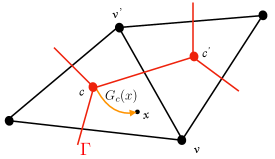
Figure 1: The two subregions/triangles $c^{*}$ and $c^{\prime*}$ with their respective reference point/center $c$ and $c^{\prime}$. $\Gamma$ is the dual 2-complex. The segment $[cc^{\prime}]$ forms a link, dual to the edge $[vv^{\prime}]$ shared by $c^{*}$ and $c^{\prime*}$. The $\operatorname{AN}$ and $\operatorname{SU}$ holonomies $\ell_{cx}$ and $h_{cx}$ are based at $c$ and go to a point $x$ in the cell $c^{*}$. These holonomies can be put together as a single ${\mathfrak{D}}_{\sigma s}$ holonomy $G_{c}(x)=\ell_{cx}h_{cx}$.

We will often omit the $x$ dependence in the notation. The solutions to the constraints are given by

$${\cal A}_{|_{c^{*}}}=\omega_{|_{c^{*}}}+e_{|_{c^{*}}}=G_{c}^{-1}\mathrm{d}G_{c}=(\ell_{c}h_{c})^{-1}\mathrm{d}(\ell_{c}h_{c}),$$ (92)

which in terms of components give (we recall that the Lie algebra $\mathfrak{an}$ is not stable under the adjoint action of $\operatorname{SU}$),

$$\omega_{|_{c^{*}}} = h_{c}^{-1}\text{d}h_{c}\>+\>\left(h_{c}^{-1}(\ell_{c}^{-1}\text{d}\ell_{c})h_{c}\right)_{|_{\mathfrak{su}}}$$ (93)

$$e_{|_{c^{*}}} = \left(h_{c}^{-1}(\ell_{c}^{-1}\text{d}\ell_{c})h_{c}\right)_{|_{\mathfrak{an}}}\,.$$ (94)

When considering an infinitesimal transformation, we recover the transformations (85) for $e=0$ and $\omega=0$. Also these solutions are the deformed version of the standard discrete picture with $\Lambda=0$ (and $n=0$),

$$\omega_{|_{c^{*}}}=h_{c}^{-1}\text{d}h_{c},\quad e_{|_{c^{*}}}=h_{c}^{-1}\mathrm{d}X\,h_{c},\quad\textrm{with }\ell\equiv X\in\mathbb{R}^{3}.$$ (95)

Before identifying the truncated symplectic form, it will be convenient to rewrite the restriction $\Omega_{|_{c}}$ of $\Omega$ to the cell $c^{*}$ as

$$\Omega_{|_{c}}=\int_{c^{*}}\left\langle\delta e\curlywedge\delta\omega\right\rangle=\tfrac{1}{2}\int_{c^{*}}\left\langle\delta{\cal A}\curlywedge\delta{\cal A}\right\rangle.$$ (96)

The truncation then imposes that ${\cal A}=G^{-1}_{c}\mathrm{d}G_{c}$.

$$\Omega_{|_{c}}\approx\Omega_{c}\equiv{\frac{1}{2}}\int_{c^{*}}\left\langle\delta(G_{c}^{-1}\mathrm{d}G_{c})\curlywedge\delta(G_{c}^{-1}\mathrm{d}G_{c})\right\rangle=\delta\Theta_{c},$$ (97)

where $\approx$ means we went on-shell, ie we truncated the number of degrees of freedom. $\Theta_{c}={\frac{1}{2}}\int_{c^{*}}\left\langle G_{c}^{-1}\mathrm{d}G_{c}\curlywedge\delta(G_{c}^{-1}\mathrm{d}G_{c})\right\rangle$ is the truncated symplectic potential.

The next steps will consist in evaluating $\sum_{i}\Omega_{c_{i}}=\sum_{i}\delta\Theta_{c_{i}}$ in order to identify the discretized variables and their phase space structure.

An important first step is to realize that what is relevant is actually the boundary data of the subregion (as we could guess already from the charge analysis in the continuum). We will be using extensively from now on the notation

$${\Delta}u:=\delta uu^{-1},\qquad{\underline{\Delta}}u:=u^{-1}\delta u$$ (98)

for some group element $u$. ${\Delta}u$ is right invariant ${\Delta}(ug)={\Delta}u$ and ${\underline{\Delta}}u$ is left invariant ${\underline{\Delta}}(gu)={\underline{\Delta}}u$, for a field independent group element $\delta g=0$.

Proposition 1

In the component connected to the identity, where ${\cal D}_{\sigma s}=\operatorname{SU}\bowtie\operatorname{AN}\ni G=\ell_{c}h_{c}$, there exist a boundary symplectic potential $\vartheta$ and a boundary Lagrangian $L_{\partial}$ given by

$$\vartheta:=-\left\langle\ell_{c}^{-1}\mathrm{d}\ell_{c},\Delta h_{c}\right\rangle,\qquad L_{\partial}:=\tfrac{1}{2}\left\langle\mathrm{d}h_{c}h_{c}^{-1}{\wedge}\ell_{c}^{-1}\mathrm{d}\ell_{c}\right\rangle,$$ (99)

such that $\Theta_{c}$ decomposes as a sum of a total derivative and a total variation

$$\Theta_{c}=\int_{c^{*}}\left(\mathrm{d}\vartheta+\delta L_{\partial}\right).$$ (100)

As a corollary we have that $\Omega_{c}=\delta\Theta_{c}=\int_{c^{*}}\mathrm{d}\delta\vartheta=\int_{\partial c^{*}}\delta\vartheta$ is a pure boundary term.

$\blacksquare$

Let us prove this proposition. We will omit the index $c$ to simplify the notation. Some useful relations are given by

$$G^{-1}\mathrm{d}G = h^{-1}\mathrm{d}h+h^{-1}(\ell^{-1}\mathrm{d}\ell)h$$ (101)

$$\delta(G^{-1}\mathrm{d}G) = h^{-1}\mathrm{d}\Delta hh+\delta(h^{-1}(\ell^{-1}\mathrm{d}\ell)h)$$ (102)

$$= h^{-1}(\mathrm{d}\Delta h+[(\ell^{-1}\mathrm{d}\ell),\Delta h]+\delta(\ell^{-1}\mathrm{d}\ell))h$$ (103)

Using these, we directly get

$$2\Theta = \int\left\langle G^{-1}\mathrm{d}G\wedge\delta(G^{-1}\mathrm{d}G)\right\rangle$$ (104)

$$= \int\left\langle(\ell^{-1}\mathrm{d}\ell)\wedge(\mathrm{d}\Delta h+[(\ell^{-1}\mathrm{d}\ell),\Delta h])\right\rangle+\left\langle h^{-1}\mathrm{d}h,\delta(h^{-1}(\ell^{-1}\mathrm{d}\ell)h)\right\rangle$$ (105)

$$= \int-\mathrm{d}\left\langle(\ell^{-1}\mathrm{d}\ell)\wedge\Delta h\right\rangle+\frac{1}{2}\left\langle[\ell^{-1}\mathrm{d}\ell,\ell^{-1}\mathrm{d}\ell]\wedge\Delta h\right\rangle$$ (107)

$$+\int\delta\left\langle\mathrm{d}hh^{-1},\ell^{-1}\mathrm{d}\ell\right\rangle-\left\langle\mathrm{d}{\Delta}h,(\ell^{-1}\mathrm{d}\ell)\right\rangle$$

$$= \int-2\mathrm{d}\left\langle(\ell^{-1}\mathrm{d}\ell)\wedge\Delta h\right\rangle+\delta\left\langle\mathrm{d}hh^{-1}\wedge(\ell^{-1}\mathrm{d}\ell)\right\rangle.$$ (108)

which establishes the result.

Therefore the symplectic form associated with a cell $c^{*}$ can be written as a sum of boundary edge contributions

$$\Omega_{|_{c}^{*}}=\delta\Theta_{|_{c}^{*}}=\delta\int_{c^{*}}\left\langle e\wedge\delta\omega\right\rangle\approx\Omega_{c}=\sum_{e\in\partial c^{*}}\Omega_{c}^{e},$$ (109)

where each contribution in the sum is given by

$$\Omega_{c}^{e}=\delta\Theta_{c}^{e},\quad\Theta_{c}^{e}:=-\int_{e}\left\langle\ell^{-1}_{c}\mathrm{d}\ell_{c},{\Delta}h_{c}\right\rangle.$$ (110)

3.2 From holonomy to ribbon and Heisenberg double

3.2.1 From holonomies to ribbons

The different subregions $c^{*}$ and $c^{\prime*}$ share some common boundaries. This common boundary is referred to as an edge $e$. This means that the variables evaluated on the edge can be related through transformations relating the different frames associated to each triangle. As we will see this will generate some simplifications in the total symplectic form $\sum_{i}\Omega_{c_{i}}$.

Let us now focus on two cells $c^{*}$ and $c^{\prime*}$, sharing the edge $e=[vv^{\prime}]$, where $v$ and $v^{\prime}$ are vertices of the cellular decomposition. As a set we have $c^{*}\cap c^{\prime*}=[vv^{\prime}]$, in addition $[vv^{\prime}]$ possesses an orientation induced by the orientation of $c$, see Fig 1. We have two contributions, for the edge $[vv^{\prime}]$ coming from the two cells sharing $[vv^{\prime}]$.

$$\Omega_{cc^{\prime}}\equiv\Omega_{c}^{[vv^{\prime}]}+\Omega_{c^{\prime}}^{[v^{\prime}v]}=\Omega_{c}^{[vv^{\prime}]}-\Omega_{c^{\prime}}^{[vv^{\prime}]},$$ (111)

where the sign changed because the edge $[vv^{\prime}]$ has a different orientation depending whether it is belonging to the boundary of $c^{*}$ or $c^{\prime*}$. On the boundary $[vv^{\prime}]$, the different fields can be combined as ${\mathfrak{D}}_{\sigma s}$ holonomies $G_{c_{i}}=\ell_{c_{i}}h_{c_{i}}$, with $\ell_{c_{i}}\in\operatorname{AN}$ and $h_{c_{i}}\in\operatorname{SU}_{\sigma s}$, are related by a ${\mathfrak{D}}_{\sigma s}$-transformation. The continuity equation states that the connection evaluated on $[vv^{\prime}]$ can be expressed either from the perspective of the frame of $c^{*}$ or the one of $c^{\prime*}$.

$${\cal A}(x)=(G_{c}^{-1}\mathrm{d}G_{c})(x)=(G_{c^{\prime}}^{-1}\mathrm{d}G_{c^{\prime}})(x),\qquad x\in[vv^{\prime}].$$ (112)

This differential equation can be integrated. Indeed, the group elements $G_{c}(x)\equiv G_{cx}$ and $G_{c^{\prime}}(x)\equiv G_{c^{\prime}x}$ are evaluated at the same point $x\in[vv^{\prime}]$ and since the connection is flat, there exists an holonomy ${\cal G}_{c^{\prime}c}=L_{c^{\prime}c}H_{c^{\prime}c}$ such that $G_{c^{\prime}}(x)={\cal G}_{c^{\prime}c}G_{c}(x)$. Note that for any given holonomy $G_{xy}$ connecting $x$ to $y$, we take the convention $G_{yx}\equiv G_{xy}^{-1}$.

The differential continuity equation is

$$\partial_{x}G_{cx}G_{xc^{\prime}}=0.$$ (113)

for $x\in[vv^{\prime}]$. This implies the integrated continuity condition

$$G_{cv}G_{vc^{\prime}}=G_{cv^{\prime}}G_{v^{\prime}c^{\prime}}.$$ (114)

Using the left Iwasawa decomposition $G_{cx}=\ell_{cx}h_{cx}$ in the cell $c^{*}$ and the right one $G_{xc^{\prime}}=h_{xc^{\prime}}\ell_{xc^{\prime}}$ in $c^{\prime*}$, we can rewrite this condition as

$$\ell_{cv}h_{cv}h_{vc^{\prime}}\ell_{vc^{\prime}}=\ell_{cv^{\prime}}h_{cv^{\prime}}h_{v^{\prime}c^{\prime}}\ell_{v^{\prime}c^{\prime}}\quad\Leftrightarrow\quad h_{cv}h_{vc^{\prime}}\ell_{vc^{\prime}}\ell_{c^{\prime}v^{\prime}}=\ell_{vc}\ell_{cv^{\prime}}h_{cv^{\prime}}h_{v^{\prime}c^{\prime}}.$$ (115)

In other words once we introduce the triangular holonomies

$$L_{vv^{\prime}}^{c}\equiv\ell_{vc}\ell_{cv^{\prime}}\in\operatorname{AN},\qquad H_{cc^{\prime}}^{v}\equiv h_{cv}h_{vc^{\prime}}\in\operatorname{SU}_{\sigma s},$$ (116)

and we can express the integrated continuity equation (114) as the ribbon structure, see Fig. 2,

$$L_{vv^{\prime}}^{c}H_{cc^{\prime}}^{v^{\prime}}=H_{cc^{\prime}}^{v}L_{vv^{\prime}}^{c^{\prime}}.$$ (117)

The triangular holonomies are the classical analogues of Kitaev’s triangle operators [73] [74].

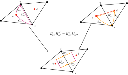
Figure 2: The constraint (117) provides the natural way to define a ribbon structure associated to each link $[cc^{\prime}]$. It encodes that the holonomy around the ribbon is trivial.

3.2.2 Heisenberg double/phase space associated to a link

Having such a ribbon structure points for a natural symplectic form [67]. In fact we are going to prove that the explicit evaluation of $\Omega_{cc^{\prime}}$, defined in (111), is the natural symplectic form making ${\mathfrak{D}}_{\sigma s}$ a Heisenberg double, the generalization of the notion of cotangent bundle as a phase space [67].

Theorem 1

The symplectic form associated to a link $[cc^{\prime}]$ is given by

$$\Omega_{cc^{\prime}} = \Omega_{c}^{{[vv^{\prime}]}}-\Omega_{c^{\prime}}^{[vv^{\prime}]}={\frac{1}{2}}\left(\left\langle{\Delta}H^{v}_{cc^{\prime}}\,\wedge\,{\Delta}L^{c}_{vv^{\prime}}\right\rangle+\left\langle{\underline{\Delta}}H^{v^{\prime}}_{cc^{\prime}}\,\wedge\,{\underline{\Delta}}L^{c^{\prime}}_{vv^{\prime}}\right\rangle\right).$$ (118)

$\blacksquare$

The proof of this result is presented in section 3.4. This theorem can be seen as the main result of the paper. Before proving the theorem it can be instructive to check that $\Omega_{cc^{\prime}}$ is indeed closed [67].

For notational simplicity, let us omit the indices and lets assume that $\ell,{\tilde{\ell}}\in\operatorname{AN}$, $h,{\tilde{h}}\in\operatorname{SU}$ are such that they form a ribbon structure

$${G\equiv\ell\,h={\tilde{h}}\,\,{\tilde{\ell}}}.$$ (119)

The 2-form $\Omega_{cc^{\prime}}=\Omega$ can then be written as

$$\Omega=\frac{1}{2}\Omega_{L}+\frac{1}{2}\Omega_{R},\qquad\Omega_{L}:=\left\langle{\Delta}{\tilde{h}}\wedge{\Delta}\ell\right\rangle,\qquad\Omega_{R}:=\left\langle{\underline{\Delta}}h\wedge{\underline{\Delta}}{\tilde{\ell}}\right\rangle,$$ (120)

The variation of this equation implies that $\Delta G={\Delta}\ell+G{\underline{\Delta}}hG^{-1}$, also that $\Delta G={\Delta}{\tilde{h}}+G{\underline{\Delta}}{\tilde{\ell}}G^{-1}$ and the identity

$${\Delta}\ell-{\Delta}{\tilde{h}} = G({\underline{\Delta}}{\tilde{\ell}}-{\underline{\Delta}}h)G^{-1}.$$ (121)

Since $\delta{\Delta}{\tilde{h}}={\Delta}{\tilde{h}}\wedge{\Delta}{\tilde{h}}$, and $\delta{\underline{\Delta}}h=-{\underline{\Delta}}h\wedge{\underline{\Delta}}h$, one finds that

$$\delta\Omega_{L} = \left\langle({\Delta}{\tilde{h}}-{\Delta}\ell)\stackrel{{\scriptstyle\wedge}}{{,}}{\Delta}{\tilde{h}}\wedge{\Delta}\ell\right\rangle$$ (122)

$$= \frac{1}{3}\left\langle({\Delta}{\tilde{h}}-{\Delta}\ell)\stackrel{{\scriptstyle\wedge}}{{,}}({\Delta}{\tilde{h}}-{\Delta}\ell)\wedge({\Delta}{\tilde{h}}-{\Delta}\ell)\right\rangle$$ (123)

We used in the second equality the fact that $\operatorname{AN}$ and $\operatorname{SU}$ are isotropic. We find a similar result for $\Omega_{R}$ with $({\Delta}{\tilde{h}}-{\Delta}\ell)$ replaced by $-({\underline{\Delta}}{\tilde{\ell}}-{\underline{\Delta}}h)$ and therefore $\delta\Omega_{R}=-\delta\Omega_{L}$, and $\Omega$ is closed. Hence the Poisson bracket associated to $\Omega_{cc^{\prime}}$ satisfies the Jacobi identity. This phase space structure generalizes the usual notion of cotangent bundle.

3.3 Drinfeld double as symmetry of the Heisenberg double

Match pair of groups.

We recall that the decompositions of ${\mathfrak{D}}_{\sigma s}$ into $\operatorname{AN}$ and $\operatorname{SU}_{\sigma s}$ provide the definitions of actions of $\operatorname{AN}$ on $\operatorname{SU}_{\sigma s}$ and vice versa. This allows to see ${\mathfrak{D}}_{\sigma s}$ as a matched pair of groups [72].

$$\ell h={\tilde{h}}{\tilde{\ell}}=(\ell\rhd h)(\ell\lhd h)\Rightarrow\ell\rhd h\equiv{\tilde{h}},\quad\ell\lhd h\equiv\tilde{\ell}$$ (124)

$${\tilde{h}}{\tilde{\ell}}=\ell h=({\tilde{h}}\rhd{\tilde{\ell}})({\tilde{h}}\lhd{\tilde{\ell}})\Rightarrow{\tilde{h}}\rhd{\tilde{\ell}}\equiv\ell,\quad{\tilde{h}}\lhd{\tilde{\ell}}\equiv h.$$ (125)

Some of the compatibility properties of the actions are as follows.

$$1\lhd h=1,\,\,\ell\lhd(h_{1}h_{2})=(\ell\lhd h_{1})\lhd h_{2},\,\,(\ell_{1}\ell_{2})\lhd h=(\ell_{1}\lhd(\ell_{2}\rhd h))(\ell_{2}\lhd h)$$

$$\ell\rhd 1=1,\,\,\ell\rhd(h_{1}h_{2})=(\ell\rhd h_{1})((\ell\lhd h_{1})\rhd h_{2}),\,\,(\ell_{1}\ell_{2})\rhd h=\ell_{1}\rhd(\ell_{2}\rhd h)$$

$$(h^{-1}\rhd\ell^{-1})={\tilde{\ell}}^{-1}=(\ell\lhd h)^{-1},\quad(h^{-1}\lhd\ell^{-1})={\tilde{h}}^{-1}=(\ell\rhd h)^{-1}$$ (126)

where we used in the last line the inverse of (119), namely $h^{-1}\ell^{-1}={\tilde{\ell}}^{-1}{\tilde{h}}^{-1}$. We have similar properties for the other actions in terms of ${\tilde{h}}$ and ${\tilde{\ell}}$.

General action of ${\mathfrak{D}}_{\sigma s}$ on itself.

The Heisenberg double is defined in terms of the group ${\mathfrak{D}}_{\sigma s}$. The group ${\mathfrak{D}}_{\sigma s}$ acts on the left (or on the right) on itself.

$$\begin{array}[]{ccc}{\mathfrak{D}}_{\sigma s}\times{\mathfrak{D}}_{\sigma s}&{\,\rightarrow}&{\mathfrak{D}}_{\sigma s}\\ (G^{\prime},G)&{\,\rightarrow}&G^{\prime}G\end{array}\qquad\begin{array}[]{ccc}{\mathfrak{D}}_{\sigma s}\times{\mathfrak{D}}_{\sigma s}&{\,\rightarrow}&{\mathfrak{D}}_{\sigma s}\\ (G^{\prime},G)&{\,\rightarrow}&GG^{\prime}\end{array}.$$ (129)

Using either of the left or right decompositions $G=\ell h={\tilde{h}}\tilde{\ell}$, and the left decomposition for $G^{\prime}=\ell^{\prime}h^{\prime}$, $\ell^{\prime}\in\operatorname{AN},\,h^{\prime}\in\operatorname{SU}_{\sigma s}$, we have, for the left action,

$$G^{\prime}G=\ell^{\prime}h^{\prime}\,\ell h=[\ell^{\prime}(h^{\prime}\rhd\ell^{\prime})][(h^{\prime}\lhd\ell)h]=\ell^{\prime}h^{\prime}{\tilde{h}}\tilde{\ell}=(\ell^{\prime}\rhd(h^{\prime}{\tilde{h}}))(\ell^{\prime}\lhd(h^{\prime}{\tilde{h}}))\tilde{\ell}.$$ (130)

The left and right actions of ${\mathfrak{D}}_{\sigma s}$ on itself encode the natural phase space symmetry actions and provide a discretization of the symmetries generated by the charges (60).

Rotations on the left.

Let us consider the infinitesimal transformations associated to left transformations (the right transformations are obtained in an analogous manner).

Let us first look at the infinitesimal (left) action $\delta^{L}_{\alpha}$ of the rotations $h^{\prime}\sim 1+\alpha$, $\alpha\in\mathfrak{su}$ on $G\in{\mathfrak{D}}_{\sigma s}$.

$$h^{\prime}{\,\triangleright\,}G=h^{\prime}G\sim(1+\alpha)G\textrm{ with }G=\ell h={\tilde{h}}\tilde{\ell}$$ (131)

We deduce then the easy transformations,

$$\delta^{L}_{\alpha}G=\alpha G,\quad\delta^{L}_{\alpha}{\tilde{h}}=\alpha{\tilde{h}},\quad\delta^{L}_{\alpha}\tilde{\ell}=0.$$ (132)

The other transformations, $\delta^{L}_{\alpha}h,\delta^{L}_{\alpha}\ell$, require a bit more work. We have

$$h^{\prime}\,\ell\,h=(h^{\prime}\rhd\ell)\,(h^{\prime}\lhd\ell)\,h\rightarrow\left|\begin{array}[]{l}h^{\prime}\rhd\ell=h^{\prime}\,\ell\,(h^{\prime}\lhd\ell)^{-1}=h^{\prime}\,\ell\,(\ell^{-1}\rhd(h^{\prime})^{-1})\\ h^{\prime}\rhd h=(h^{\prime}\lhd\ell)\,h\end{array}\right..$$ (135)

So at the infinitesimal level, we have

$$\delta^{L}_{\alpha}\ell = \alpha\ell-\ell(\alpha\lhd\ell),$$ (136)

$$\delta^{L}_{\alpha}h = (\alpha\lhd\ell)\,h.$$ (137)

Since we deal with a match pair of groups, due to the action and back action we can have a twisted compatibility relation with the product [72]. In particular for the action on the $\operatorname{AN}$ sector we have,

$$h\rhd(\ell_{1}\ell_{2})=(h\rhd\ell_{1})((h\lhd\ell_{1})\rhd\ell_{2}){\,\rightarrow\,}\delta_{\alpha}(\ell_{1}\ell_{2})=(\delta_{\alpha}\ell_{1})\ell_{2}+\ell_{1}(\delta_{\alpha\lhd\ell_{1}}\ell_{2}).$$ (138)

The action (136) satisfies such condition.

$$\delta_{\alpha}(\ell_{1}\ell_{2}) = \alpha\ell_{1}\ell_{2}-\ell_{1}\ell_{2}(\alpha\lhd(\ell_{1}\ell_{2}))$$ (139)

$$= \{(\alpha\ell_{1})-\ell_{1}(\alpha\lhd\ell_{1})\}\ell_{2}+\ell_{1}\{(\alpha\lhd\ell_{1})\ell_{2}-\ell_{2}((\alpha\lhd\ell_{1})\lhd\ell_{2})\}$$

$$= (\delta_{\alpha}\ell_{1})\ell_{2}+\ell_{1}(\delta_{\alpha\lhd\ell_{1}}\ell_{2}).$$

Charge for the rotations on the left.

In the continuum picture we have identified the charges $J^{\prime}$ generating the rotational symmetry. The following proposition determines the corresponding charge in the discrete picture.

Proposition 2

The triangular holonomy $\ell=L^{c}_{vv^{\prime}}$ generates the infinitesimal left rotations.

$$\delta^{L}_{\alpha}\lrcorner\,\Omega_{cc^{\prime}} = \left\langle\alpha\,,\,{\Delta}\ell\right\rangle.$$ (140)

We provide the proof in Appendix B.1. Geometrically this (infinitesimal) rotation is located at $c$ as it can be read from (132), remembering that $\tilde{\ell}=L^{c^{\prime}}_{vv^{\prime}}$ and ${\tilde{h}}=H^{v}_{cc^{\prime}}$.

Generating left rotations with Poisson brackets.

The Poisson bracket associated to the symplectic form can be obtained by inverting the symplectic form [67]. We can also directly infer it from the infinitesimal transformations. Indeed, as discussed in [75], since $\ell$ is the charge of the left rotation $\delta^{L}_{\alpha}$ we can recover from the action of $\delta^{L}_{\alpha}$ on $(\ell,{\tilde{\ell}},h,{\tilde{h}})$ the Poisson bracket of $\ell$ with all the other components, using the correspondence

$$\delta^{L}_{\alpha}\cdot=-\left\langle\alpha\,,\,\{\ell_{1}\,,\,\cdot\}\ell_{1}^{-1}\right\rangle_{1},$$ (141)

where we are using here the notation $\ell_{1}:=\ell{\otimes}1$, $\ell_{2}:=1{\otimes}\ell$ and $\left\langle,\right\rangle_{1}$ means we are contracting the first sector of the tensor product.

Proposition 3

The Poisson brackets implementing the infinitesimal transformation (141) can be conveniently written in terms of the $r$-matrix [76]

$$r_{-}\equiv-\tau_{I}{\otimes}{{\bf J}}^{I}.$$ (142)

and are given by

$$\{\ell_{1},\ell_{2}\}=[r_{-},\ell_{1}\ell_{2}], \{\ell_{1},h_{2}\}=\ell_{1}r_{-}h_{2},$$ (143)

$$\{\ell_{1},\tilde{\ell}_{2}\}=0, \,\,\{\ell_{1},{\tilde{h}}_{2}\}=r_{-}\,\ell_{1}{\tilde{h}}_{2}.$$

We provide the proof in Appendix B.2.

Translations on the left.

A similar calculation can be performed for the infinitesimal (left) translations $\delta^{L}_{\phi}$, $\operatorname{AN}\ni\ell^{\prime}\sim 1+\phi$, $\phi\in\mathfrak{an}$.

$$\ell^{\prime}{\,\triangleright\,}G=\ell^{\prime}G\sim(1+\phi)G\textrm{ with }G=\ell h={\tilde{h}}\tilde{\ell}$$ (144)

We deduce again the easy transformations,

$$\delta^{L}_{\phi}G=\phi G,\quad\delta^{L}_{\phi}\ell=\phi\ell,\quad\delta^{L}_{\phi}h=0,$$ (145)

and the other transformations, $\delta^{L}_{\phi}{\tilde{h}},\delta^{L}_{\phi}\tilde{\ell}$, require a bit more work. We have

$$\,{\tilde{h}}\,\tilde{\ell}\,=(\ell^{\prime}\rhd{\tilde{h}})\,(\ell^{\prime}\lhd{\tilde{h}})\,\tilde{\ell}\rightarrow\left|\begin{array}[]{l}\ell^{\prime}\rhd{\tilde{h}}=\ell^{\prime}\,{\tilde{h}}\,(\ell^{\prime}\lhd{\tilde{h}})^{-1}=\ell^{\prime}\,{\tilde{h}}\,({\tilde{h}}^{-1}\rhd m^{-1})\\ \ell^{\prime}\rhd\tilde{\ell}=(\ell^{\prime}\lhd{\tilde{h}})\,\tilde{\ell}\end{array}\right..$$ (148)

We note that the formulae are actually very similar to the left rotations we first determined. It is natural since the construction is by essence symmetric between the $\mathfrak{su}$ and $\mathfrak{an}$ sectors.

At the infinitesimal level, we have

$$\delta^{L}_{\phi}{\tilde{h}} = \phi{\tilde{h}}-{\tilde{h}}({\tilde{h}}^{-1}\rhd\phi)=\phi{\tilde{h}}-{\tilde{h}}(\phi\lhd{\tilde{h}}),$$ (149)

$$\delta^{L}_{\phi}\tilde{\ell} = (\phi\lhd{\tilde{h}})\,\tilde{\ell}.$$ (150)

It is clear that the action (149) satisfies a twisted compatibility condition with the product of $\operatorname{SU}$, since the formula is very similar to (136).

Charge for the translations on the left.

In the continuum picture we have identified the charges generating the translation symmetry $P^{\prime}$. The following proposition determines the corresponding charge in the discrete picture. As one could expect, the charge generating the left translation is now given by the $\operatorname{SU}$ holonomy.

Proposition 4

The triangular holonomy ${\tilde{h}}=H^{v}_{cc^{\prime}}$ generates the infinitesimal left translations.

$$\delta^{L}_{\phi}\lrcorner\,\Omega_{cc^{\prime}} = -\left\langle\phi,\,{\Delta}{\tilde{h}}\,\right\rangle.$$ (151)

The proof of this proposition is very close to the one of Proposition 2, thanks to the symmetric treatment between the variables $\ell\leftrightarrow{\tilde{h}}$, $\tilde{\ell}\leftrightarrow h$, and sectors $\mathfrak{an}\leftrightarrow\mathfrak{su}$. Geometrically this (infinitesimal) translation is based at $v$, as it can be read from (145), remembering that $\ell=L^{c}_{vv^{\prime}}$ and $h=H^{v^{\prime}}_{cc^{\prime}}$.

Generating left translations with Poisson brackets.

We can also derive the infinitesimal translations using the Poisson bracket.

$$\delta^{L}_{\phi}\cdot=\left\langle\phi\,,\,\{{\tilde{h}}_{1}\,,\,\cdot\}{\tilde{h}}_{1}^{-1}\right\rangle_{1}.$$ (152)

The difference of minus sign with respect to (141) is due to the fact that the charges have opposite sign as one can see looking at (151) and (140).

Proposition 5

The Poisson brackets implementing the infinitesimal transformation (152) can be conveniently written in terms of the $R$-matrix [76]

$$r_{+}=J_{I}{\otimes}\tau^{I},$$ (153)

and are given by

$$\{{\tilde{h}}_{1},{\tilde{h}}_{2}\}=[r_{+},{\tilde{h}}_{1}{\tilde{h}}_{2}],\quad\{{\tilde{h}}_{1},\tilde{\ell}_{2}\}={\tilde{h}}_{1}r_{+}\tilde{\ell}_{2},\quad\{{\tilde{h}}_{1}\,,\,h_{2}\}=0,\quad\{{\tilde{h}}_{1}\,,\,\ell_{2}\}=r_{+}{\tilde{h}}_{1}\ell_{2}.$$ (154)

The proof is given in Appendix B.3. It is very similar to the earlier proof of proposition 3 due to the symmetry between the sectors $\operatorname{SU}$ and $\operatorname{AN}$ in the different decompositions.

A similar construction can be done for the infinitesimal right translations and rotations, which are respectively generated by $H_{cc^{\prime}}^{v^{\prime}}=h$ and $L^{c^{\prime}}_{vv^{\prime}}=\tilde{\ell}$ and act respectively at $v^{\prime}$ and $c^{\prime}$. Determining these infinitesimal transformations allows to find the missing Poisson brackets, such as in particular

$$\{h_{1},h_{2}\}=-[r_{+},h_{1}h_{2}],\qquad\{h_{1},\tilde{\ell}_{2}\}=-h_{1}\tilde{\ell}_{2}r_{+},\qquad\{\tilde{\ell}_{1},\tilde{\ell}_{2}\}=-[r_{-},\tilde{\ell}_{1}\tilde{\ell}_{2}].$$ (155)

These can be obtained by the correspondence ${\tilde{h}}^{-1}\to h$. In summary we find that the Heisenberg poisson brackets when restricted to the variables $(h,\ell)$ are

$$\{\ell_{1},\ell_{2}\}=[r_{-},\ell_{1}\ell_{2}],\qquad\{\ell_{1},h_{2}\}=\ell_{1}r_{-}h_{2},\qquad\{h_{1},h_{2}\}=-[r_{-},h_{1}h_{2}].$$ (156)

Finite transformations.

We can also look at the finite version of the left or right transformations. These are obtained from the group ${\mathfrak{D}}_{\sigma s}$ acting on itself as we have discussed earlier (129). We can prove that they are phase space symmetries if we equip the group ${\mathfrak{D}}_{\sigma s}$ with another Poisson structure, which this time is not invertible (it is however compatible with the group product of ${\mathfrak{D}}_{\sigma s}$). In this case, ${\mathfrak{D}}_{\sigma s}$ as a symmetry group is called the Drinfled double. In order to write these we note that the r-matrices $(r_{+},r_{-})$ satisfy the relations

$$2r:=r_{+}+r_{-},\qquad r_{+}-r_{-}=C$$ (157)

where $C$ is the quadratic Casimir of ${\mathfrak{d}}$ and we have introduced the antisymmetric $r$-matrix $r$.

$$\textrm{\,\,\,\,Heisenberg double :}\{G_{1},G_{2}\}=[r,{G{\otimes}G}]_{+}={rG{\otimes}G}+{G{\otimes}G}r,$$ (158)

$$\textrm{Drinfeld double :}\{G^{\prime}_{1},G^{\prime}_{2}\}=[r,G^{\prime}{\otimes}G^{\prime}]_{-}={rG^{\prime}{\otimes}G^{\prime}}-{G^{\prime}{\otimes}G^{\prime}}r,$$ (159)

with $G,G^{\prime}\in{\mathfrak{D}}_{\sigma s}$ . The set of Poisson brackets we just derived in (156) are equivalent to the Poisson brackets (158). On the other hand the Poisson brackets given in (159) are simply [76],

$$\{\ell^{\prime}_{1},\ell^{\prime}_{2}\}=[r_{-},\ell^{\prime}_{1}\ell^{\prime}_{2}],\qquad\{\ell^{\prime}_{1},h^{\prime}_{2}\}=0=\{h^{\prime}_{1},\ell^{\prime}_{2}\},\qquad\{h^{\prime}_{1},h^{\prime}_{2}\}=[r_{+},h^{\prime}_{1}h^{\prime}_{2}].$$ (160)

The left or right action of ${\mathfrak{D}}_{\sigma s}$ as a Drinfeld double on ${\mathfrak{D}}_{\sigma s}$ as a Heisenberg double is a Poisson map [76]. This means in physical terms that our phase space structure is covariant under the action of the Drinfeld double, which encodes some symmetry transformations equipped with a (in general non-trivial) Poisson structure. Upon quantization, the non-trivial Poisson structure becomes the relevant non-commutative/quantum group structure. Our quantum mechanical states being built from representations of these symmetries will then be naturally defined in terms of quantum group representations. We will come back to this point in Section 4.

3.4 Proof of the main result

Let us prove here the main result of the paper given by theorem 1. We start from the discretized symplectic form on the boundary of the cell $c$. Within any cell $c^{*}$ we have from Proposition 1 that

$$\Theta_{|_{c}}=\int_{c^{*}}\left\langle e\wedge\delta\omega\right\rangle\approx\Theta_{c}=\sum_{[vv^{\prime}]\in\partial c^{*}}\Theta_{c}^{[vv^{\prime}]},\quad\Theta_{c}^{[vv^{\prime}]}=-\int_{[vv^{\prime}]}\delta\left\langle\ell_{c}^{-1}\mathrm{d}\ell_{c}\wedge{\Delta}h_{c}\right\rangle.$$ (161)

Given two cells $c^{*},c^{\prime*}$ one defines the holonomy $G_{cc^{\prime}}=L_{cc^{\prime}}H_{cc^{\prime}}$ and denote $G_{cx}=\ell_{cx}h_{cx}$, $G_{xc}=G_{cx}^{-1}$. We also denote, for any holonomy $u_{ab}$ from to $a$ to $b$, $u^{-1}_{ab}=u_{ba}$. Given $x\in[vv^{\prime}]$, one defines

$$H^{x}_{c^{\prime}c}\equiv h_{c^{\prime}x}h_{xc},\qquad{\tilde{\ell}}_{cx}\equiv L_{cc^{\prime}}\ell_{c^{\prime}x}.$$ (162)

Taking the variation of the first equation of (162), we get

$${\Delta}h_{c^{\prime}x} = \Delta H^{x}_{c^{\prime}c}+H^{x}_{c^{\prime}c}\Delta h_{cx}H^{x}_{cc^{\prime}}=H^{x}_{c^{\prime}c}({\Delta}h_{cx}-{\Delta}H^{x}_{cc^{\prime}})(H^{x}_{c^{\prime}c})^{-1},$$ (163)

where we have used that ${\Delta}H^{-1}=-H^{-1}{\Delta}HH$. Taking the differential of the second relation in (162) gives

$$\ell_{c^{\prime}x}^{-1}\mathrm{d}\ell_{c^{\prime}x}={\tilde{\ell}}_{cx}^{-1}\mathrm{d}{\tilde{\ell}}_{cx}.$$ (164)

The continuity equations across the edge $[vv^{\prime}]$ separating $c$ from $c^{\prime}$ is equivalent to an exchange relation:

$$G_{c^{\prime}c}G_{cx}=G_{c^{\prime}x},\quad\Leftrightarrow\quad H_{c^{\prime}c}\ell_{cx}={\tilde{\ell}}_{cx}H^{x}_{c^{\prime}c}.$$ (165)

Taking the differential of the continuity equation (165), we get

$${\tilde{\ell}}_{cx}^{-1}\mathrm{d}{\tilde{\ell}}_{cx} = \left(H^{x}_{c^{\prime}c}(\ell_{cx}^{-1}\mathrm{d}\ell_{cx})H^{x}_{cc^{\prime}}+H^{x}_{c^{\prime}c}\mathrm{d}H^{x}_{cc^{\prime}}\right).$$ (166)

This relation, together with (163,164) allows us to relate the contribution of the cell $c^{\prime}$ to the one of the cell $c$. Denoting $\Theta_{cc^{\prime}}=\Theta_{c}^{[vv^{\prime}]}-\Theta_{c^{\prime}}^{[vv^{\prime}]}$ with $\Theta_{c}^{e}:=-\int_{e}\left\langle\ell^{-1}_{cx}\mathrm{d}\ell_{cx},{\Delta}h_{cx}\right\rangle$, see (110), one finds that

$$\Theta_{cc^{\prime}}=-\int_{[vv^{\prime}]}\left\langle\ell_{cx}^{-1}\mathrm{d}\ell_{cx}{,}\left({\Delta}H^{x}_{cc^{\prime}}\right)\right\rangle=\int_{[vv^{\prime}]}\left\langle{\tilde{\ell}}_{cx}^{-1}\mathrm{d}{\tilde{\ell}}_{cx}{,}\left({\Delta}H^{x}_{c^{\prime}c}\right)\right\rangle.$$ (167)

The second equality is due to the differential continuity equation (166) and the identity ${\underline{\Delta}}H=H^{-1}{\Delta}HH=-{\Delta}H^{-1}$. The fact that there are two equivalent expressions for the symplectic potential simply follows from the exchange $c\leftrightarrow c^{\prime}$. Under this exchange $\Theta_{cc^{\prime}}$ is antisymmetric. It is also clear from the continuity equation written as ${\tilde{\ell}}_{cx}^{-1}H_{c^{\prime}c}\ell_{cx}=H^{x}_{c^{\prime}c}$ that under this exchange we have ${\tilde{\ell}}_{c}\leftrightarrow\ell_{c}$.

The variation of the differential continuity (166) gives

$$H^{x}_{cc^{\prime}}\delta({\tilde{\ell}}_{cx}^{-1}\mathrm{d}{\tilde{\ell}}_{cx})H^{x}_{c^{\prime}c}-\delta(\ell_{cx}^{-1}\mathrm{d}\ell_{cx}) = \left([\ell_{cx}^{-1}\mathrm{d}\ell_{cx},\Delta H^{x}_{cc^{\prime}}]+\mathrm{d}{\Delta}H^{x}_{cc^{\prime}}\right).$$ (168)

One can use this to establish that

$$\delta\left\langle(\ell_{cx}^{-1}\mathrm{d}\ell_{cx}){\Delta}H^{x}_{cc^{\prime}}\right\rangle = \left\langle\delta(\ell_{cx}^{-1}\mathrm{d}\ell_{cx})\curlywedge{\Delta}H^{x}_{cc^{\prime}}\right\rangle+\left\langle[\ell_{cx}^{-1}\mathrm{d}\ell_{cx}{,}{\Delta}H^{x}_{cc^{\prime}}]\curlywedge{\Delta}H^{x}_{cc^{\prime}}\right\rangle$$ (169)

$$= \left\langle H^{x}_{cc^{\prime}}\delta({\tilde{\ell}}_{cx}^{-1}\mathrm{d}{\tilde{\ell}}_{cx})H^{x}_{c^{\prime}c}\curlywedge{\Delta}H^{x}_{cc^{\prime}}\right\rangle$$ (170)

$$= -\left\langle\delta({\tilde{\ell}}_{cx}^{-1}\mathrm{d}{\tilde{\ell}}_{cx})\curlywedge{\Delta}H^{x}_{c^{\prime}c}\right\rangle.$$ (171)

where we have denoted $\curlywedge$ the variational wedge product. This means that

$$\Omega_{cc^{\prime}} = \int_{[vv^{\prime}]}\left\langle\delta({\tilde{\ell}}_{cx}^{-1}\mathrm{d}{\tilde{\ell}}_{cx})\curlywedge{\Delta}H^{x}_{c^{\prime}c}\right\rangle=-\int_{[vv^{\prime}]}\left\langle\delta(\ell_{cx}^{-1}\mathrm{d}\ell_{cx})\curlywedge\Delta H^{x}_{cc^{\prime}}\right\rangle.$$ (172)

From the variation of the continuity equation (165) one gets

$${\Delta}H^{x}_{cc^{\prime}} = {\underline{\Delta}}\ell_{cx}+\ell_{xc}{\underline{\Delta}}H_{c^{\prime}c}\ell_{cx}+\ell_{xc}H_{cc^{\prime}}{\underline{\Delta}}{\tilde{\ell}}_{xc}H_{c^{\prime}c}\ell_{cx}$$ (173)

$$= \ell_{c}^{-1}\left\{H_{cc^{\prime}}({\Delta}{\tilde{\ell}}_{c})H_{c^{\prime}c}+{\Delta}H_{cc^{\prime}}-{\Delta}\ell_{c}\right\}\ell_{c},$$ (174)

where we have used that ${\underline{\Delta}}H^{-1}=-{\Delta}H$. Similarly we have an equivalent variational continuity identity obtained by exchanging $c\leftrightarrow c^{\prime}$ and $\ell_{c}\leftrightarrow{\tilde{\ell}}_{c}$

$${\Delta}H^{x}_{c^{\prime}c} = {\tilde{\ell}}_{c}^{-1}\left\{H_{c^{\prime}c}({\Delta}\ell_{c})H_{cc^{\prime}}+{\Delta}H_{c^{\prime}c}-{\Delta}{\tilde{\ell}}_{c}\right\}{\tilde{\ell}}_{c}.$$ (175)

Using these relations and the fact that $\delta(\ell_{c}^{-1}\mathrm{d}\ell_{c})=\ell_{c}^{-1}(\mathrm{d}\Delta\ell_{c})\ell_{c}$ one can evaluate (172)

$$\Omega_{cc^{\prime}} = -\int_{[vv^{\prime}]}\left\langle\mathrm{d}{\Delta}\ell_{c}\curlywedge\left(H_{cc^{\prime}}({\Delta}{\tilde{\ell}}_{c})H_{c^{\prime}c}+{\Delta}H_{cc^{\prime}}\right)\right\rangle,$$ (176)

$$= \int_{[vv^{\prime}]}\left\langle\mathrm{d}{\Delta}{\tilde{\ell}}_{c}\curlywedge\left(H_{c^{\prime}c}({\Delta}\ell_{c})H_{cc^{\prime}}+{\Delta}H_{c^{\prime}c}\right)\right\rangle.$$ (177)

Note that we repeatedly use the fact that the subalgebra $\mathfrak{su}$ or $\mathfrak{an}$ are isotropic with respect to our scalar product. Quite remarkably the integrant of $\Omega_{cc^{\prime}}$ is a total differential. This can be simply seen by taking the sum of ((176)) and ((177)) which gives after integration

$$\Omega_{cc^{\prime}}=-\frac{1}{2}\left.\left(\left\langle{\Delta}\ell_{c}\curlywedge{\Delta}H_{cc^{\prime}}\right\rangle+\left\langle{\Delta}\ell_{c}\curlywedge H_{cc^{\prime}}({\Delta}{\tilde{\ell}}_{c})H_{c^{\prime}c}\right\rangle+\left\langle{\Delta}H_{c^{\prime}c}\curlywedge{\Delta}{\tilde{\ell}}_{c}\right\rangle\right)\right|_{x=v}^{x=v^{\prime}}.$$ (178)

To evaluate this expression one recall the definition of the triangular holonomies

$$L_{vv^{\prime}}^{c}=\ell_{vc}\ell_{cv^{\prime}},\qquad L_{v^{\prime}v}^{c^{\prime}}={\tilde{\ell}}_{v^{\prime}c}{\tilde{\ell}}_{cv}.$$ (179)

Taking their variation gives

$$({\Delta}\ell_{cv^{\prime}}-{\Delta}\ell_{cv})=\ell_{cv}\,({\Delta}L_{vv^{\prime}}^{c})\,\ell_{cv}^{-1},\qquad({\Delta}{\tilde{\ell}}_{cv^{\prime}}-{\Delta}{\tilde{\ell}}_{cv})=-{\tilde{\ell}}_{cv^{\prime}}\,({\Delta}L_{v^{\prime}v}^{c^{\prime}})\,{\tilde{\ell}}_{cv^{\prime}}^{-1}.$$ (180)

By adding a vanishing contribution $\left\langle{\Delta}\ell_{cv^{\prime}}\curlywedge H_{cc^{\prime}}{\Delta}{\tilde{\ell}}_{cv}H_{cc^{\prime}}^{-1}\right\rangle-\left\langle{\Delta}\ell_{cv^{\prime}}\curlywedge H_{cc^{\prime}}{\Delta}{\tilde{\ell}}_{cv}H_{cc^{\prime}}^{-1}\right\rangle$ to (178), we obtain

$$-2\Omega_{cc^{\prime}} = \left\langle({\Delta}\ell_{cv^{\prime}}-{\Delta}\ell_{cv})\wedge({\Delta}H_{cc^{\prime}}+H_{cc^{\prime}}{\Delta}{\tilde{\ell}}_{cv}H_{cc^{\prime}}^{-1})\right\rangle$$ (181)

$$+ \left\langle{\Delta}H_{c^{\prime}c}\curlywedge({\Delta}{\tilde{\ell}}_{cv^{\prime}}-{\Delta}{\tilde{\ell}}_{cv})\right\rangle+\left\langle{\Delta}\ell_{cv^{\prime}}\wedge H_{cc^{\prime}}({\Delta}{\tilde{\ell}}_{cv^{\prime}}-{\Delta}{\tilde{\ell}}_{cv})H_{cc^{\prime}}^{-1}\right\rangle$$

$$= \left\langle\,({\Delta}L^{c}_{vv^{\prime}})\,\curlywedge\ell_{cv}^{-1}({\Delta}H_{cc^{\prime}}+H_{cc^{\prime}}{\Delta}{\tilde{\ell}}_{cv}H_{cc^{\prime}})\ell_{cv}\right\rangle$$

$$- \left\langle{\tilde{\ell}}_{cv^{\prime}}^{-1}({\Delta}H_{c^{\prime}c}+H_{c^{\prime}c}{\Delta}\ell_{cv^{\prime}}H_{cc^{\prime}}){\tilde{\ell}}_{cv^{\prime}}\curlywedge\,({\Delta}L_{v^{\prime}v}^{c^{\prime}})\,\right\rangle$$

We can now use the variational continuity equations (173) at $x=v^{\prime}$ and (175) at $x=v$, to get the simple expression

$$2\Omega_{cc^{\prime}} = -\left\langle\,{\Delta}L^{c}_{vv^{\prime}}\,\curlywedge{\Delta}H_{cc^{\prime}}^{v}\right\rangle+\left\langle{\Delta}H_{c^{\prime}c}^{v^{\prime}}\curlywedge\,{\Delta}L_{v^{\prime}v}^{c^{\prime}}\,\right\rangle$$ (182)

$$= \left\langle{\Delta}H_{cc^{\prime}}^{v}\curlywedge{\Delta}L^{c}_{vv^{\prime}}\right\rangle+\left\langle{\underline{\Delta}}H_{cc^{\prime}}^{v^{\prime}}\curlywedge\,{\underline{\Delta}}L_{vv^{\prime}}^{c^{\prime}}\,\right\rangle,$$ (183)

which is the desired result.

3.5 Ribbon network as the classical version of the quantum group spin network

Let us recall that we consider a cellular decomposition $\Gamma^{*}$ of the 2d manifold $\Sigma$. We denote $\Gamma$ the dual 2-complex, made of nodes, links and faces. Let us see how the model is now built in terms of the discretized variables. We focus, in this section, on the Euclidean case with $\Lambda<0$, since the Iwasawa decomposition is global in this case.

First the links are glued to each other at a node. For each link, we have a ribbon, hence we need to glue the ribbons together. By construction, the triangular holonomies in the $\operatorname{AN}$ sector going around a cell (eg a triangle) have a product which is the identity (as we assumed there is no torsion defect).

$${\cal L}^{c}=L^{c}_{vv^{\prime}}L^{c}_{v^{\prime}v^{\prime\prime}}L^{c}_{v^{\prime\prime}v}=\ell_{vc}\ell_{cv^{\prime}}\ell_{v^{\prime}c}\ell_{cv^{\prime\prime}}\ell_{v^{\prime\prime}c}\ell_{cv}=1.$$ (184)

This indicates that the three ribbons ends form a closed $\operatorname{AN}$ holonomy and tells us how the ribbon are glued together, see Fig. 3. This is the analogue of the Gauss constraint.

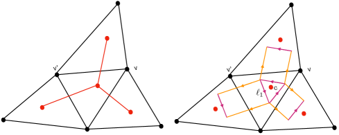
Figure 3: The ribbon data encodes all the geometric data. In particular, when the ribbons meet at a node, the Gauss constraint $\ell_{1}\ell_{2}\ell_{3}=L^{c}_{v^{\prime\prime}v}L^{c}_{v^{\prime}v^{\prime\prime}}L^{c}_{vv^{\prime}}=1$ encodes the gauge invariance at the node and is the generalization of the flat case $X_{1}+X_{2}+X_{3}=0$.

Once the ribbons are glued together, we can also look at the faces generated by the“long side” of the ribbon. Provided there is no curvature excitation, we expect to have a product of $\operatorname{SU}$ holonomies associated to the links $l_{i}$ around $v$ (or said otherwise the links which form the boundary of face $v^{*}$) being equal to the identity.

$${\cal G}^{v}=\prod_{l_{i}\in\partial v^{*}}\left(H^{v}_{l_{i}}\right)^{\pm 1}=1,$$ (185)

where $\pm 1$ depends on the orientation of the link $l_{i}$.

These two sets of constraints provide the discretization of the (global) charges (52). As we have seen in Section 3.3, these two sets of holonomies generate the discrete analogue of the gauge transformations and the translations, as expected. Hence they should be seen as a discretization fo the charges $J^{\prime}$ and $P^{\prime}$ given in (52), for constant transformation parameters on the boundary. Alternatively, one can check how the constraints ${\cal L}^{c}$, ${\cal G}^{v}$ can be viewed as a discretization of the generalized torsion and curvature constraints (81), (80) (with no matter source).

Proposition 6

The holonomies $L^{c}_{vv^{\prime}}$, $H^{v}_{cc^{\prime}}$ are related to the (infinitesimal) continuum charges in the following way, with $h_{cx}$ a $\operatorname{SU}$ holonomy connecting $c$ to $x$ a point in the relevant path.

$$L^{c}_{vv^{\prime}}={\cal P}\exp\left(\int_{[vv^{\prime}]}h_{cx}{\,\triangleright\,}e(x)\right),$$ (186)

$$H^{v}_{cc^{\prime}}={\cal P}\exp\left(\int_{[vv^{\prime}]}\omega(x)-\left(h_{cx}^{-1}\,(h_{cx}\rhd e(x))\,h_{cx}\right)_{|_{\mathfrak{su}}}\right)$$ (187)

The discrete constraints ${\cal L}^{c}=L^{c}_{vv^{\prime}}L^{c}_{v^{\prime}v^{\prime\prime}}L^{c}_{v^{\prime\prime}v}=1$, ${\cal G}^{v}=H^{v}_{cc^{\prime}}..H^{v}_{c^{(n)}c}=1$ encode that the generalized torsion and curvature are zero.

$${\cal L}^{c}=1 \Leftrightarrow \mathrm{d}e+\omega\rhd e+{\frac{1}{2}}[e\wedge e]_{\mathfrak{an}}=0$$ (188)

$${\cal G}^{v}=1 \Leftrightarrow \mathrm{d}\omega+\omega\lhd e+{\frac{1}{2}}[\omega\wedge\omega]_{\mathfrak{su}}=0.$$ (189)

We leave the proof of the proposition in Appendix B.4. The expression of the discretized variables in terms of the continuum fields when $\Lambda\neq 0$ is another aspect of the main result of this paper.

The (generalized) LQG phase space is given in terms of the product of phase space ${\mathfrak{D}}_{\sigma s}^{l_{i}}$ associated to the links $l_{i}=[c_{i}c_{i+1}]$, quotiented by the action of the (Gauss) constraints ${\cal L}^{c^{i}}\equiv\prod_{j}L^{c^{i}}_{v_{j}v_{j+1}}$ acting at the nodes $c_{i}$.

$${\cal P}:=\times_{i}{\mathfrak{D}}_{\sigma s}^{l_{i}}/\!/{\cal L}^{c_{i}}$$ (190)

The dynamics is given in terms of the contraints ${\cal G}^{v}$ associated to the vertices $v_{i}$ of $\Gamma^{*}$, expressed in terms of the $H^{v_{i}}$.

This model is exactly the model discussed in [68]. The ribbon structure was proposed to define the classical phase space structure of 3d gravity in the presence of a cosmological constant. Here this model is derived rigorously from the continuum. Note that [77] analyzed how such model can be related to the Fock-Rosly approach to the Chern-Simons formulation (in the case of the torus space).

4 Recovering the quantum group structure

The quantum theory associated to the Heisenberg double phase space in the $\operatorname{SU}_{\sigma s}$ case is a standard construction leading to the appearance of quantum group [16]. For the sake of being complete let us recall the construction without going through all the technical details (see also [31] in the $\operatorname{SU}(2)$ case). Again, we focus on ${\mathfrak{D}}_{+-}=\operatorname{SL}(2,\mathbb{C})=\operatorname{SU}(2)\bowtie\operatorname{AN}$, the Euclidean case with $\Lambda<0$.

Constructing a quantum theory means that we use a representation of the relevant symmetries, which we saw in Sections 2 and 3.3 were associated to charges. In the case of 3d gravity, we have two types of symmetries, the rotation symmetries and the translations. While in the full theory we need to implement both, the order in which we implement them at the quantum level matters. The different options are first the rotations then the translations, or vice versa, or both at the same time. The first approach consists in the LQG picture, the second one is ”dual LQG” [78], and the third one is the Chern-Simons picture.

In the following we will focus on the LQG approach, meaning that we will implement the rotational symmetry first, encoded by the Gauss charges.

4.1 Poisson-Lie symmetry

Before proceeding to quantization we need to tie one lose end. The relationship between the $r$-matrix $r$ entering the Poisson brackets and the $r$-matrix ${\mathfrak{r}}$ entering the deformation of the action. These are given by

$$r_{-}=-\tau_{I}{\otimes}{{\bf J}}^{I}\in\mathfrak{an}{\otimes}\mathfrak{su},\qquad{\mathfrak{r}}={\mathfrak{r}}_{IJ}{{\bf J}}^{I}{\otimes}{{\bf J}}^{J}\in\mathfrak{su}{\otimes}\mathfrak{su}.$$ (191)

We have seen in (156) that the Poisson brackets of the rotational holonomies is given by

$$\{h_{1},h_{2}\}=-[r_{-},h_{1}h_{2}].$$ (192)

We expect however that the charge of symmetries acting on our phase space to belong the the Poisson-Lie group SU. This possesses the Poisson commutation relations

$$\{h_{1},h_{2}\}=[{\mathfrak{r}},h_{1}h_{2}].$$ (193)

There seems to be a tension between this two results. This tension is simply resolved by the fact that these two expressions are the same.

$$[{\mathfrak{r}},h_{1}h_{2}]=-[r_{-},h_{1}h_{2}]$$ (194)

Strikingly this shows that the $r$-matrix we have introduced at the very beginning as a boundary term (2.1) enters as a structure constant deforming the symmmetry group action. ${\mathfrak{r}}$ is the standard $r$-matrix encoding the deformation of the group $\operatorname{SU}(2)$ [76], [16]. Our construction highlights that the notion of quantum group appears from the addition of the specific boundary term in (2.1).

One first establish it at the level of the Lie algebra: Given $\alpha\in\mathfrak{su}$ we want to prove that

$$[{\mathfrak{r}},\alpha_{1}+\alpha_{2}]=-[r_{-},\alpha_{1}+\alpha_{2}].$$ (195)

This can be established by a direct computation as shown in [16]. For the reader’s convenience we present it here explicitly. Taking $\alpha={{\bf J}}^{I}$, and using (68) and (65), we have

$$-[r_{-},{{\bf J}}^{I}{\otimes}1+1{\otimes}{{\bf J}}^{I}] = [\tau_{J},{{\bf J}}^{I}]{\otimes}{{\bf J}}^{J}-\tau_{J}{\otimes}[{{\bf J}}^{J},{{\bf J}}^{I}]$$ (196)

$$= -(C_{JK}{}^{I}{{\bf J}}^{K}+\epsilon^{I}{}_{J}{}^{K}\tau_{K}){\otimes}{{\bf J}}^{J}-\tau_{J}{\otimes}(\epsilon^{JI}{}_{K}{{\bf J}}^{K}),$$ (197)

$$= C_{JK}{}^{I}{{\bf J}}^{J}\otimes{{\bf J}}^{K}$$ (198)

$$= \sigma[(n\cdot{{\bf J}})\otimes{{\bf J}}^{I}-{{\bf J}}^{I}{\otimes}(n\cdot{{\bf J}})].$$ (199)

while on the other hand we have

$$[{\mathfrak{r}},{{\bf J}}^{I}{\otimes}1+1{\otimes}{{\bf J}}^{I}] = {\mathfrak{r}}_{AB}\left([{{\bf J}}^{A},{{\bf J}}^{I}]{\otimes}{{\bf J}}^{B}+{{\bf J}}^{A}{\otimes}[{{\bf J}}^{B},{{\bf J}}^{I}]\right)$$ (200)

$$= \left({\mathfrak{r}}_{AB}\epsilon^{AIC}\right)({{\bf J}}_{C}{\otimes}{{\bf J}}^{B}-{{\bf J}}^{B}{\otimes}{{\bf J}}_{C})$$ (201)

$$= n^{D}\epsilon_{DAB}\epsilon^{AIC}({{\bf J}}_{C}{\otimes}{{\bf J}}^{B}-{{\bf J}}^{B}{\otimes}{{\bf J}}_{C})$$ (202)

$$= \sigma n^{D}(\delta_{B}^{I}\delta_{D}^{C}-\delta_{B}^{C}\delta_{D}^{I})({{\bf J}}_{C}{\otimes}{{\bf J}}^{B}-{{\bf J}}^{B}{\otimes}{{\bf J}}_{C})$$ (203)

$$= \sigma[(n\cdot{{\bf J}}){\otimes}{{\bf J}}^{I}-{{\bf J}}^{I}{\otimes}(n\cdot{{\bf J}})].$$ (204)

This establishes (195). The identity (194) follows by exponentiation.

4.2 Quantization

Specific representation choice.

It is useful to choose a specific representation to make some explicit calculations. An element $\ell$ in $\operatorname{AN}$ will be specified by a real number $\lambda$ and a complex number $z$.

$$\ell\equiv\begin{pmatrix}\lambda&0\\ z&\lambda^{-1}\end{pmatrix},\quad\bar{\ell}\equiv\begin{pmatrix}\lambda^{-1}&-\overline{z}\\ 0&\lambda\end{pmatrix}.$$ (205)

Note however that this representation is not faithful for $\operatorname{AN}$ so this is why we need to consider also $\bar{\ell}\equiv\ell^{\dagger-1}$. (The map $G\to\bar{G}={G}^{\dagger-1}$ is a group morphism of $\operatorname{AN}$, which leaves the rotation subgroup invariant, as can be seen from the Iwasawa decomposition $\ell h{\,\rightarrow\,}h^{\dagger}\ell^{\dagger}{\,\rightarrow\,}\ell^{\dagger-1}h^{\dagger-1}=\bar{\ell}h$ [31].) It is convenient to consider dimensionless Lie algebra generators, $(\sigma^{I},\xi_{I}=i\sigma_{I}+(\sigma\times\hat{n})_{I})$, where $\hat{n}=(0,0,1)$ is the (dimensionless) normalized vector, and $\sigma_{I}$ are the (hermitian) Pauli matrices with $[\sigma_{I},\sigma_{J}]=i\,\epsilon_{IJ}{}^{K}\sigma_{K}$.

$${{\bf J}}^{I}=-i\kappa\,\sigma^{I},\quad\tau_{I}=i\sqrt{|\Lambda|}\xi_{I}.$$ (206)

This means in particular that the $r$-matrix parametrizing the Poisson brackets will have an explicit parameter dependence (not hidden in the Lie algebra generators anymore as in section 3.3), given by $\gamma={\kappa}\sqrt{|\Lambda|}$. This leads to an explicit expression for the $r$-matrix.

$$r_{-}\,=\,-\tau^{I}{\otimes}{{\bf J}}_{I}\,=-\,\gamma\,\xi^{I}{\otimes}\sigma_{I}=i\frac{\gamma}{4}\begin{pmatrix}-1&0&0&0\\ 0&1&0&0\\ 0&-4&1&0\\ 0&0&0&-1\end{pmatrix}.$$ (207)

We recall that for a given link, we have the ribbon variables $\ell\in\operatorname{AN}$, with Poisson brackets

$$\{\ell_{1},\ell_{2}\}=[r_{-},\ell_{1}\ell_{2}],\quad\{\bar{\ell}_{1},\bar{\ell}_{2}\}=[r_{-},\bar{\ell}_{1}\bar{\ell}_{2}],\quad\{\ell_{1},\bar{\ell}_{2}\}=[r_{-},\ell_{1}\bar{\ell}_{2}].$$ (208)

These are equivalent to the following Poisson commutation relations

$$\{\lambda,z\}=i\frac{\gamma}{2}{z}\lambda,\qquad\{\lambda,\bar{z}\}=-i\frac{\gamma}{2}{\bar{z}}\lambda,\qquad\{\bar{z},z\}=-i\gamma(\lambda^{2}-\lambda^{-2}).$$ (209)

while other commutators vanish.

Quantization.

Let us quantize the matrix elements of $\ell$, so that they become operators [79, 31]. We first introduce the parameter

$$q=e^{\hbar\gamma/2},\textrm{ with }\hbar\gamma=\hbar\kappa\sqrt{|\Lambda|}=8\pi\frac{l_{P}}{l_{c}},$$ (210)

where $l_{P}=\hbar G$ is the Planck length and $l_{C}=|\Lambda|^{-{\frac{1}{2}}}$ is the cosmological scale.

We define then the deformed quantum monodromy matrix

$$\ell{\,\rightarrow\,}\hat{\ell}=\begin{pmatrix}K&0\\ (q-q^{-1})J_{+}&K^{-1}\end{pmatrix},\quad\bar{\ell}{\,\rightarrow\,}\hat{\bar{\ell}}=\begin{pmatrix}K^{-1}&-(q-q^{-1})J_{-}\\ 0&K\end{pmatrix},$$ (211)

where the correspondence is

$$K=\hat{\lambda},\quad(q-q^{-1})J_{+}=\hat{z},\qquad-(q-q^{-1})J_{-}=\hat{\bar{z}}.$$ (212)

The classical $r$-matrix becomes the quantum $R$-matrix

$$r_{-}{\,\rightarrow\,}R_{-}=q^{-\frac{1}{2}}\begin{pmatrix}q&0&0&0\\ 0&1&0&0\\ 0&(q-q^{-1})&1&0\\ 0&0&0&q\end{pmatrix}={\bf 1}+i\hbar\,r_{-}+\mathcal{O}(\hbar^{2}).$$ (213)

Finally the Poisson brackets which appears though the limit $[\hat{\ell}_{1},\hat{\ell}_{2}]\to-i\hbar\{{\ell}_{1},{\ell}_{2}\}$, are quantized through

$$R_{-}\,\hat{\ell}_{1}\,\hat{\ell}_{2}=\hat{\ell}_{2}\,\hat{\ell}_{1}\,R_{-} {\,\rightarrow\,} \{\ell_{1},\ell_{2}\}=[r_{-},\ell_{1}\ell_{2}],$$

$$R_{-}\,\hat{\bar{\ell}}_{1}\,\hat{\bar{\ell}}_{2}=\hat{\bar{\ell}}_{2}\,\hat{\bar{\ell}}_{1}\,R_{-} {\,\rightarrow\,} \{{\bar{\ell}}_{1},{\bar{\ell}}_{2}\}=[r_{-},{\bar{\ell}}_{1}{\bar{\ell}}_{2}],$$

$$R_{-}\,\hat{\ell}_{1}\,\hat{\bar{\ell}}_{2}=\hat{\bar{\ell}}_{2}\,\hat{\ell}_{1}\,R_{-} {\,\rightarrow\,} \{\ell_{1},{\bar{\ell}}_{2}\}=[r_{-},\ell_{1}{\bar{\ell}}_{2}].$$ (214)

In components, the commutation relations on the right hand side of (4.2) read

$$K\,J_{+}\,K^{-1}=q\,J_{+},\qquad K\,J_{-}\,K^{-1}=q^{-1}\,J_{-},\qquad[J_{+},J_{-}]=\frac{K^{2}-K^{-2}}{q-q^{-1}}.$$ (215)

These are the commutation relations of $\mathcal{U}_{q}(\operatorname{SU}(2))$. This is encoding the well-known fact that the quantum algebra of functions on $\operatorname{AN}$ is isomorphic to the algebra $\mathcal{U}_{q}(\operatorname{SU}(2))$.

The last element we need is the Hilbert space. Since we intend first to implement the rotational symmetries, we consider the natural Hilbert space associated to the $\hat{\ell}$ which actually span $\mathcal{U}_{q}(\operatorname{SU}(2))$. Hence we consider the Hilbert space given in terms of the irreducible representations of $\mathcal{U}_{q}(\operatorname{SU}(2))$. Strictly speaking we should consider such Hilbert space for a half link, and glue two of such representations to build a full link as recalled in [78]. We will skip these subtleties here.

Now that we have the quantum theory for a given link, we need to extend the structure to the full graph $\Gamma$. For simplicity we have taken $\Gamma^{*}$ to be a triangulation so that the nodes of $\Gamma$ are trivalent. For each node, we have three $\operatorname{AN}$ holonomies, belonging to different phase spaces, which product is $1$. This is the Gauss law. The product is given by the matrix product.

The quantum version of the Gauss law is direct. Since we have to consider three phase spaces, we have to deal with three Hilbert space copies, with each quantum $\operatorname{AN}$ holonomy acting a given Hilbert space. The $\operatorname{AN}$ holonomies are multiplied using the matrix product, hence the natural quantization of the holonomy product is

$$(\ell\ell^{\prime})_{ik}=\sum_{j}(\ell)_{ij}(\ell^{\prime})_{jk}{\,\rightarrow\,}(\widehat{\ell\ell^{\prime}})_{ik}\equiv\sum_{j}(\widehat{\ell})_{ij}{\otimes}(\widehat{\ell})_{jk}={\Delta}\widehat{\ell}_{ik}.$$ (216)

This is nothing else than the natural coproduct for the algebra of functions on $\operatorname{AN}$. We read in terms of the components,

$${\Delta}\widehat{\ell}=\begin{pmatrix}K\otimes K&0\\ (q-q^{-1})(J_{+}\otimes K+K^{-1}\otimes J_{+})&K^{-1}\otimes K^{-1}\end{pmatrix},$$ (217)

and $${\Delta}\hat{\bar{\ell}}=\begin{pmatrix}K\otimes K&-(q-q^{-1})(J_{-}\otimes K+K^{-1}\otimes J_{-})\\ 0&K^{-1}\otimes K^{-1}\end{pmatrix}.$$

We recognize the coproduct of $\mathcal{U}_{q}(\operatorname{SU}(2))$. The Gauss constraint demanding that the product of the three $\operatorname{AN}$ holonomies is 1 is then quantized as

$$1_{ik}=(\ell\ell^{\prime}\ell^{\prime\prime})_{ik}=\sum_{jl}\ell_{ij}\ell^{\prime}_{jl}\ell^{\prime\prime}_{lk}{\,\rightarrow\,}\sum_{jl}\widehat{\ell}_{ij}{\otimes}\widehat{\ell}_{jl}{\otimes}\widehat{\ell}_{lk}=(1{\otimes}{\Delta})\circ{\Delta}\widehat{\ell}_{ik}=\widehat{1}_{ik}.$$ (218)

The elements in the Hilbert space solutions of such constraints are the $\mathcal{U}_{q}(\operatorname{SU}(2))$ intertwiners, generated by the deformed Clebsh-Gordan coefficients. We recover in this way the $\mathcal{U}_{q}(\operatorname{SU}(2))$ spin networks. Solving then the last set of constraints for the $\operatorname{SU}(2)$ holonomies gives rise to the Turaev-Viro amplitude [80].

Outlook

In this work we investigated why, at the quantum level, a deformed gauge symmetry, parametrized by the cosmological constant $\Lambda$, appears whereas the original action for 3d gravity is a plain undeformed gauge theory.

The first key insight was to realize that we had to perform a change of variables at the continuum level, in order to have a Gauss constraint/rotational charge algebra depending upon the cosmological constant. The change of variables is a simple canonical transformation parametrized by a vector $n$ which equivalently can be seen as induced by a boundary term. Such vector $n$ is taken as a scalar (ie an invariant) for the gauge symmetries and therefore leads to a modification of the realization of the symmetries. Since $n$ is constrained to depend on $\Lambda$, we do get symmetries that depend on $\Lambda$ at the action level.

This is yet another example that the choice of variables matters in the quest of defining a proper quantum gravity theory. There is an obvious parallel in our work and the 4d LQG approach where one performs a canonical transformation parameterized by a scalar, the Immirzi parameter or equivalently adds a (topological) term not modifying the equations of motion, the Holst term to define the Ashtekar-Barbero variables. This canonical transformation renders the theory more amenable to discretization, just like our term does for 3d gravity. The main difference however is that $n$ is parameterized by $\Lambda$ so it is not really adding an extra parameter in the theory unlike the Immirzi parameter.

The second key insight is the discretization procedure. It is in fact a subtle procedure: we have decomposed the system into subsystems and managed to project all the degrees of freedom on the boundary of the subsystems by imposing an appropriate truncation of the degrees of freedom. Such truncation is obtained by going on-shell. In the 3d gravity context, this amounts to consider region of homogeneous curvature and no torsion. This is essentially the same as dealing with the notion of ”geometric structures”[69] or equivalently homogeneously curved polygons. A boundary shared by two polygons can be viewed from the perspective of each polygon, and an isometry relating the two, the so-called continuity equations. This allowed to express the discrete variables solely in terms of ”corner” terms (the classical version of the Kitaev triangle operators [73] [74]). From this perspective, the quantum group symmetry appears in a sense as the ”corner term contributions”. Note also that our work shares some similarities with the seminal works [32][33], where the quantum group symmetry is identified at the classical level for the Wess-Zumino model.

The phase space associated to each link of the graph $\Gamma$ (dual to the triangulation $\Gamma^{*}$) now depends on the cosmological constant $\Lambda$. Importantly, we have derived this phase space (the Heisenberg double) starting from the continuum symplectic form. It was already known that such Heisenberg double equipped with the appropriate constraints, provides a discretization of 3d gravity with a non-vanishing cosmological constant [68] and also leads upon quantization to deformed spin networks and the TV amplitude [31]. We have therefore found the missing link connecting the discretized model and the continuum model. This paper provides therefore a long thought-for and rigorous derivation of the quantum group structure – as a kinematical symmetry– in the 3d loop quantum gravity case. Interestingly it can also provide the link between the Fock-Rosly approach and the gravity continuum variables, since it was explicitly shown in [77] how such approach was related to the ribbon model [68].

This works opens many new avenues of investigation. Let us review some of them.

More general vector $n$.

There is some room to go beyond the quantum group case, by removing some conditions on the vector $n$,

$$\delta n=0,\quad n^{2}=-\Lambda^{2},\quad\mathrm{d}n=0,\quad n^{I}=(0,0,n^{3}).$$ (219)

We can consider for example a vector such $\mathrm{d}n\neq 0$, which would generate some new central extension (55) that would be interesting to explore.

In our construction, the vector $n$ is a scalar for the symmetries, with its norm fixed by the cosmological constant. Hence in a sense, the only relevant information we keep about $n$ is its norm. It would be interesting to see how its direction could also be relevant. For example, two vectors $n$, related by a rotation lead to isomorphic quantum group structures. At the classical level a rotation of the vectors corresponds to a canonical transformation. It would be interesting to see whether this is the case at the quantum group level. That is is it possible to relate explicitly two rotated quantum group structure by a unitary transformation?

Unexplored cases.

For the sake of simplicity, we focused on the simplest cases. Indeed as we argued earlier, the Euclidean case with positive cosmological constant has to be treated separately due to appearance of reality conditions since we have to deal with a complex $n$.

In the Lorentzian cases, we focused on the component connected to the identity to use the Iwasawa decomposition, $\ell h={\tilde{h}}{\tilde{\ell}}$, but one should deal with the general case, where there exist $d_{i},d_{j}\in{\mathfrak{d}}_{-,s}$, such that $\ell d_{i}h={\tilde{h}}d_{j}^{-1}{\tilde{\ell}}$. The Heisenberg double can be generalized accordingly [67]. This amounts however to decorate the ribbon by some curvature parametrized by $d_{i}$.

We have studied only one polarization choice in the discretization in section 3. Namely we looked at the case where $\operatorname{AN}$ holonomies are associated to the edges whereas the $\operatorname{SU}$ holonomies are associated to the links. Due to the symmetric treatment between the two groups, we can actually swap the location of the holonomies. In fact the continuity equation (114) also allows to identify the dual variables.

$$G_{cv}G_{vc^{\prime}}=G_{cv^{\prime}}G_{v^{\prime}c^{\prime}}\Leftrightarrow\quad\tilde{L}^{v}_{cc^{\prime}}\tilde{H}^{c^{\prime}}_{vv^{\prime}}=\tilde{H}^{c}_{vv^{\prime}}\tilde{L}^{v^{\prime}}_{cc^{\prime}}.$$ (220)

Hence we have $\tilde{L}^{x}_{cc^{\prime}}\in\operatorname{AN}$, with $x$ being $v$ or $v^{\prime}$, associated to the links and $\tilde{H}^{y}_{vv^{\prime}}\in\operatorname{SU}$, with $y$ being $c$ or $c^{\prime}$, associated to the edges. This provides a deformation of the dual loop formalism [60, 62], which should be the classical analogue of [59] (for the case $q$ real though). We leave the study of this other polarization for later studies.

It is clear that our construction can be generalized to any factorizable group. Namely, considering a BF theory associated with a simple Lie group $G$, we expect the boundary deformation to be given in terms of the standard $r$-matrix and the main results and proofs to generalize seamlessly. We leave this for future work.

Adding matter.

While we did not introduce matter, in the shape of curvature or torsion excitations, the formalism can certainly be extended to this case. We expect that the edge mode (or corner terms) perspective provides naturally the notion of particles in the curved case, just like it did in the flat case [61].

We expect then to recover a version of the Kitaev model, defined for (deformation of) Lie groups. It would be then interesting to explore how much gravity questions we could ask in the Kitaev model context. This would develop some new interplay between models of (topological) quantum information theory and quantum gravity.

4d case.

The case of real interest is certainly the 4d case and one can expect that our approach here is also relevant in this context. Indeed, preliminary calculations show that one can perform an analogue change of variables to remove the volume term in the action and to have some $\Lambda$ dependent gauge transformations. This would provide hints on the proper deformation one would expect in the 4d case. According to the signature and sign of the cosmological constant, there might be also some non-trivial interplays with the time gauge. This question is currently being addressed.

Acknowledgements

This research was supported in part by Perimeter Institute for Theoretical Physics. Research at Perimeter Institute is supported by the Government of Canada through the Department of Innovation, Science and Economic Development Canada and by the Province of Ontario through the Ministry of Research, Innovation and Science. A. O. is supported by the NSERC Discovery grants held by M. D. and F. G.

Appendix A Playing with cross and dot products

A.1 Poisson algebra of charges

We explicitly calculate the Poisson bracket between the different charges generating the deformed symmetries. We work with ${\kappa}=1$.

$$\{{P^{\prime}}_{\alpha},P^{\prime}_{\beta}\} = \{P_{\alpha}+J_{\alpha\times n},P_{\beta}+J_{\beta\times n}\}$$ (221)

$$= \sigma\Lambda J_{\alpha\times\beta}+P_{(\alpha\times n)\times\beta-(\beta\times n)\times\alpha}+J_{(\alpha\times n)\times(\beta\times n)}\quad{\scriptscriptstyle\alpha\times(\beta\times n)-\beta\times(\alpha\times n)=(\alpha\times\beta)\times n}$$ (222)

$$= (\sigma\Lambda+\sigma n^{2})J_{\alpha\times\beta}+P_{(\alpha\times\beta)\times n}+J_{((\alpha\times\beta)\times n)\times n}\quad{\scriptscriptstyle(\alpha\times n)\times(\beta\times n)=((\alpha\times\beta)\times n)\times n+\sigma n^{2}(\alpha\times\beta)}$$ (223)

$$= (\sigma\Lambda+\sigma n^{2})J^{\prime}_{\alpha\times\beta}+P^{\prime}_{(\alpha\times\beta)\times n}$$ (224)

$$\{J^{\prime}_{\alpha},P^{\prime}_{\beta}\} = \{J_{\alpha},P_{\beta}+J_{\beta\times n}\}$$ (225)

$$= P_{\alpha\times\beta}+J_{\alpha\times(\beta\times n)}$$ (226)

$$= {P}_{\alpha\times\beta}+J_{\beta\times(\alpha\times n)}+J_{(\alpha\times\beta)\times n}\quad{\scriptscriptstyle\alpha\times(\beta\times n)-\beta\times(\alpha\times n)=(\alpha\times\beta)\times n}$$ (227)

$$= P^{\prime}_{\alpha\times\beta}+J^{\prime}_{\beta\times(\alpha\times n)}$$ (228)

A.2 ${\mathfrak{d}}_{\sigma s}$ gauge theory.

Let us consider the ${\mathfrak{d}}$ connection ${\cal A}=\omega+e$, then the curvature of ${\cal A}$ is

$$F[{\cal A}] = \mathrm{d}{\cal A}+{\frac{1}{2}}[{\cal A}\wedge{\cal A}]=\mathrm{d}\omega+\mathrm{d}e+{\frac{1}{2}}[(\omega+e)\wedge(\omega+e)]$$ (229)

$$= \mathrm{d}\omega+\mathrm{d}e+{\frac{1}{2}}[\omega\wedge\omega]+{\frac{1}{2}}[e\wedge e]+[\omega\wedge e]$$

$$= \mathrm{d}\omega+\mathrm{d}e+{\frac{1}{2}}[\omega\wedge\omega]+{\frac{1}{2}}[e\wedge e]+\omega\rhd e+\omega\lhd e$$

$$= (\mathrm{d}\omega+{\frac{1}{2}}[\omega\wedge\omega]+\omega\lhd e)+(\mathrm{d}e+{\frac{1}{2}}[e\wedge e]+\omega\rhd e)$$

which is the sum of the generalized curvature in the $\mathfrak{su}$ direction and the generalized torsion in the $\mathfrak{an}$ sector.

To determine the derivative in the different sectors, we consider the ${\mathfrak{d}}_{\sigma s}$ element $\psi=\alpha+\phi$, $\alpha\in\mathfrak{su}$ and $\phi\in\mathfrak{an}$,

$$\mathrm{d}_{\cal A}\psi = \mathrm{d}\alpha+\mathrm{d}\phi+[(\omega+e),(\alpha+\phi)]$$ (230)

$$= (\mathrm{d}\alpha+[\omega,\alpha]+\omega\lhd\phi+e\rhd\alpha)+(\mathrm{d}\phi+[e,\phi]+\omega\rhd\phi+e\lhd\alpha)$$ (231)

Setting either of $\alpha$ or $\phi$ to be zero, we get the derivative in the respective directions.

$$D\alpha = \mathrm{d}\alpha+[\omega,\alpha]_{\mathfrak{su}}+e\rhd\alpha$$ (232)

$$= \mathrm{d}\alpha+\omega\times\alpha+e\times(n\times\alpha)$$ (233)

$$\tilde{D}\phi = \mathrm{d}\phi+[e,\phi]_{\mathfrak{an}}+\omega\rhd\phi$$ (234)

$$= \mathrm{d}\phi+(e\times\phi)\times n+\omega\times\phi$$ (235)

These derivative satisfy the metric compatibility condition

$$\mathrm{d}(\alpha\cdot\phi)=D\alpha\cdot\phi+\alpha\cdot\tilde{D}\phi,$$ (236)

which can be shown directly using the definition of the vector triple product $(\alpha\times\beta)\times n=\sigma[(\alpha\cdot n)\beta-\alpha(n\cdot\beta)].$

Appendix B Some proofs

B.1 Proof of Proposition 2

We want to prove that

$$\delta^{L}_{\alpha}\lrcorner\,\Omega_{cc^{\prime}} = \left\langle\alpha\,,\,{\Delta}\ell\right\rangle$$ (237)

It is actually only necessary to use (132) in the symplectic form to identify the charge generating the infinitesimal rotations. The following identities will be useful to do the proof.

$${\tilde{h}}^{-1}\ell h=\tilde{\ell} \Leftrightarrow {\underline{\Delta}}\tilde{\ell}=h^{-1}(\ell^{-1}{\underline{\Delta}}{\tilde{h}}\ell+{\underline{\Delta}}\ell+{\Delta}h)h$$

$$\left\langle h^{-1}\delta^{L}_{\alpha}h\,,\,{\underline{\Delta}}\tilde{\ell}\right\rangle = \left\langle\delta^{L}_{\alpha}hh^{-1}\,,\,(\ell^{-1}{\underline{\Delta}}{\tilde{h}}^{-1}\ell+{\underline{\Delta}}\ell+{\Delta}h)\right\rangle$$

$$= \left\langle\delta^{L}_{\alpha}hh^{-1}\,,\,\ell{}^{-1}(-{\Delta}h+{\Delta}\ell)\ell\right\rangle$$

With this in mind the calculation is direct.

$$\delta^{L}_{\alpha}\lrcorner\,\Omega_{cc^{\prime}} = {\frac{1}{2}}\left(\left\langle\delta^{L}_{\alpha}{\tilde{h}}{\tilde{h}}^{-1}\,,\,{\Delta}\ell\right\rangle+\left\langle\delta^{L}_{\alpha}hh^{-1}\,,\,h{\underline{\Delta}}\tilde{\ell}h^{-1}\right\rangle-\left\langle{\Delta}{\tilde{h}}\,,\,\delta^{L}_{\alpha}\ell\ell^{-1}\right\rangle\right)$$ (238)

$$= {\frac{1}{2}}\left(\left\langle\delta^{L}_{\alpha}{\tilde{h}}{\tilde{h}}^{-1}\,,\,{\Delta}\ell\right\rangle+\left\langle\delta^{L}_{\alpha}hh^{-1}\,,\,\ell^{-1}(-{\Delta}{\tilde{h}}+{\Delta}\ell)\ell\right\rangle-\left\langle{\Delta}{\tilde{h}}\,,\,\delta^{L}_{\alpha}\ell\ell^{-1}\right\rangle\right)$$

$$= {\frac{1}{2}}\left(\left\langle\delta^{L}_{\alpha}{\tilde{h}}{\tilde{h}}^{-1}+\ell\delta^{L}_{\alpha}hh^{-1}\ell^{-1}\,,\,{\Delta}\ell\right\rangle-\left\langle\delta^{L}_{\alpha}\ell\ell^{-1}+\ell\delta^{L}_{\alpha}hh^{-1}\ell^{-1}\,,\,{\Delta}{\tilde{h}}\right\rangle\right)$$

$$= {\frac{1}{2}}\left(\left\langle\alpha+\delta^{L}_{\alpha}GG^{-1}-\delta^{L}_{\alpha}\ell\ell^{-1}\,,\,{\Delta}\ell\right\rangle-\left\langle\delta^{L}_{\alpha}GG^{-1}\,,\,{\Delta}{\tilde{h}}\right\rangle\right)$$

$$= \left\langle\alpha\,,\,{\Delta}\ell\right\rangle-{\frac{1}{2}}\left\langle\alpha\,,\,{\Delta}{\tilde{h}}\right\rangle$$

$$= \left\langle\alpha\,,\,{\Delta}\ell\right\rangle$$

B.2 Proof of Proposition 3

We want to prove that the Poisson brackets

$$\{\ell_{1},\ell_{2}\}=[r_{-},\ell_{1}\ell_{2}], \{\ell_{1},h_{2}\}=\ell_{1}r_{-}h_{2},\,\,$$ (239)

$$\{\ell_{1},\tilde{\ell}_{2}\}=0, \,\,\{\ell_{1},{\tilde{h}}_{2}\}=r_{-}\,\ell_{1}{\tilde{h}}_{2}.$$

with $r_{-}=-\tau_{I}{\otimes}{{\bf J}}^{I}$ are the right brackets to generate the infinitesimal transformations, through the formula

$$\delta^{L}_{\alpha}\cdot=-\left\langle\alpha_{1}+\phi_{1}\,,\,\{\ell_{1}\,,\,\cdot\}\ell_{1}^{-1}\right\rangle_{1},$$ (240)

where $\alpha\in\mathfrak{su}$ and $\phi\in\mathfrak{an}$. The fact that $\phi$ is projected out is necessary to interpret $\{\ell_{1}\,,\,\cdot\}\ell_{1}^{-1}$ as a vector field in AN.

The proof goes as follows

$$-\left\langle\alpha_{1}+\phi_{1}\,,\,\{\ell_{1}\,,\,\ell_{2}\}\ell_{1}^{-1}\right\rangle_{1} = -\left\langle\alpha_{1}+\phi_{1}\,,\,[r_{-},\ell_{1}\ell_{2}]\ell_{1}^{-1}\right\rangle_{1}$$

$$= \left\langle(\alpha+\phi),\tau_{I}\right\rangle{{\bf J}}^{I}\ell-\left\langle(\alpha+\phi),\ell\tau_{I}\ell^{-1}\right\rangle\ell{{\bf J}}^{I}$$

$$= \alpha\ell-\left\langle\ell^{-1}\alpha\ell\,,\,\tau_{I}\right\rangle\ell{{\bf J}}^{I}=\alpha\ell-(\alpha\lhd\ell)_{I}\ell{{\bf J}}^{I}$$

$$= \alpha\ell-\ell(\alpha\lhd\ell)=\delta^{L}_{\alpha}\ell,$$ (242)

where we used that $\alpha\lhd\ell=(\ell^{-1}\alpha\ell)_{|_{\mathfrak{su}}}=\left\langle\ell^{-1}\alpha\ell\,,\,\tau_{I}\right\rangle{{\bf J}}^{I}$ and that $\left\langle\ell^{-1}\phi\ell\,,\,\tau_{I}\right\rangle=0$.

Similarly, taking

$$-\left\langle\alpha_{1}+\phi_{1}\,,\,\{\ell_{1}\,,\,h_{2}\}\ell_{1}^{-1}\right\rangle_{1} = -\left\langle\alpha_{1}+\phi_{1}\,,\,\ell_{1}\,r_{-}\,h_{2}\ell_{1}^{-1}\right\rangle_{1}$$

$$= \left\langle\alpha+\phi\,,\,\ell\tau_{I}\ell^{-1}\right\rangle{{\bf J}}^{I}h$$

$$= (\ell^{-1}\alpha\ell)_{|_{\mathfrak{su}}}h=(\alpha\lhd\ell)h=\delta^{L}_{\alpha}h$$ (244)

Finally

$$-\left\langle\alpha_{1}+\phi_{1}\,,\,\{\ell_{1}\,,\,{\tilde{h}}_{2}\}\ell_{1}^{-1}\right\rangle_{1} = -\left\langle\alpha\,,\,r_{-}\,{\tilde{h}}_{2}\right\rangle_{1}$$ (245)

$$= \left\langle\alpha+\phi\,,\,\tau_{I}\right\rangle{{\bf J}}^{I}{\tilde{h}}=\alpha h=\delta^{L}_{\alpha}{\tilde{h}},$$ (246)

while

$$\{\ell_{1},\tilde{\ell}_{2}\}=0 {\,\rightarrow\,} \delta^{L}_{\alpha}\tilde{\ell}=0.$$ (247)

which completes the proof.

B.3 Proof of Proposition 5

We want to prove that the Poisson brackets

$$\{{\tilde{h}}_{1},{\tilde{h}}_{2}\}=[r_{+},{\tilde{h}}_{1}{\tilde{h}}_{2}],\quad\{{\tilde{h}}_{1},\tilde{\ell}_{2}\}={\tilde{h}}_{1}r_{+}\tilde{\ell}_{2},\quad\{{\tilde{h}}_{1}\,,\,h_{2}\}=0,\quad\{{\tilde{h}}_{1}\,,\,\ell_{2}\}=r_{+}{\tilde{h}}_{1}\ell_{2}.$$ (248)

are the right brackets to generate the infinitesimal transformations, through the formula

$$\delta^{L}_{\phi}\cdot=\left\langle\alpha_{1}+\phi_{1}\,,\,\{{\tilde{h}}_{1}\,,\,\cdot\}{\tilde{h}}_{1}^{-1}\right\rangle_{1},$$ (249)

where $\alpha\in\mathfrak{su}$ and $\phi\in\mathfrak{an}$.

The proof goes as follows. First

$$\delta^{L}_{\phi}{\tilde{h}} = \left\langle\alpha_{1}+\phi_{1}\,,\,\{{\tilde{h}}_{1}\,,\,{\tilde{h}}_{2}\}{\tilde{h}}_{1}^{-1}\right\rangle_{1}=\left\langle\alpha_{1}+\phi_{1}\,,\,[r_{+},{\tilde{h}}_{1}{\tilde{h}}_{2}]{\tilde{h}}_{1}^{-1}\right\rangle_{1}$$ (250)

$$= \left\langle\alpha_{1}+\phi_{1}\,,\,{{\bf J}}_{I}\right\rangle\tau^{I}{\tilde{h}}-\left\langle\alpha_{1}+\phi_{1}\,,{\tilde{h}}{{\bf J}}_{I}{\tilde{h}}^{-1}\right\rangle{\tilde{h}}\tau^{I}=\phi{\tilde{h}}-{\tilde{h}}({\tilde{h}}^{-1}\phi{\tilde{h}})_{|_{\mathfrak{an}}}$$

$$= \phi{\tilde{h}}-{\tilde{h}}(\phi\lhd{\tilde{h}}).$$

Then the other proofs are direct.

$$\{{\tilde{h}}_{1},\tilde{\ell}_{2}\}={\tilde{h}}_{1}r_{+}\tilde{\ell}_{2} {\,\rightarrow\,} \delta^{L}_{\phi}\tilde{\ell}({\tilde{h}}^{-1}\phi{\tilde{h}})_{|_{\mathfrak{an}}}\tilde{\ell}=(\phi\lhd{\tilde{h}}){\tilde{h}}$$ (251)

$$\{{\tilde{h}}_{1}\,,\,h_{2}\}=0 {\,\rightarrow\,} \delta^{L}_{\phi}h=0$$ (252)

$$\{{\tilde{h}}_{1}\,,\,\ell_{2}\}=r_{+}{\tilde{h}}_{1}\ell_{2} {\,\rightarrow\,} \delta^{L}_{\phi}\ell=\phi\ell.$$ (253)

B.4 Proof of Proposition 6

First we want to find the relation between the discrete charges and the continuum ones. Let us consider the $\operatorname{AN}$ holonomy $L^{c}_{vv^{\prime}}=\ell_{vc}\ell_{cv^{\prime}}$. It is enough to focus on the single holonomy $\ell_{cx}$ for $x\in[vv^{\prime}]$, as in Fig. 1. We can express $\ell_{cx}$ in terms of the $\mathfrak{an}$ connection ${\overline{\textbf{e}}}(y)\equiv\ell_{cy}^{-1}\mathrm{d}\ell_{cy}$.

$$\ell_{cx}={\cal P}\exp\left(\int_{cx}{\overline{\textbf{e}}}\right).$$ (254)

In a similar way, we can define a $\operatorname{SU}$ holonomy $h$ and connection ${\overline{\omega}}(y)\equiv h_{cy}^{-1}\mathrm{d}h_{cy}$.

$$h_{cx}={\cal P}\exp\left(\int_{cx}{\overline{\omega}}\right).$$ (255)

The connections ${\overline{\omega}},{\overline{\textbf{e}}}$ are actually related to the spin connection $\omega$ and frame field $e$. Recall that we took in (93), (94), omitting the subscripts $cy$,

$$\omega^{I}{{\bf J}}_{I} \equiv h^{-1}\text{d}h\>+\>\left(h^{-1}(\ell^{-1}\text{d}\ell)h\right)_{|_{\mathfrak{su}}}={\overline{\omega}}\>+\>\left(h^{-1}\,{\overline{\textbf{e}}}\,h\right)_{|_{\mathfrak{su}}}$$ (256)

$$e_{I}\tau_{I} \equiv \left(h^{-1}\,(\ell^{-1}\text{d}\ell)\,h\right)_{|_{\mathfrak{an}}}=\left(h^{-1}\,{\overline{\textbf{e}}}\,h\right)_{|_{\mathfrak{an}}}\equiv h^{-1}{\,\triangleright\,}{\overline{\textbf{e}}}\,.$$ (257)

The action we defined $h{\,\triangleright\,}{\overline{\textbf{e}}}=\left(h\,{\overline{\textbf{e}}}\,h^{-1}\right)_{|_{\mathfrak{an}}}$ is indeed an action since

$$g\left(h\,{\overline{\textbf{e}}}\,h^{-1}\right)g^{-1} = \left((gh)\,{\overline{\textbf{e}}}\,(gh)^{-1}\right)_{|_{\mathfrak{an}}}+\left((gh)\,{\overline{\textbf{e}}}\,(gh)^{-1}\right)_{|_{\mathfrak{su}}}=(gh)\rhd{\overline{\textbf{e}}}+\left((gh)\,{\overline{\textbf{e}}}\,(gh)^{-1}\right)_{|_{\mathfrak{su}}}$$

$$= g\left(h\,{\overline{\textbf{e}}}\,h^{-1}\right)_{|_{\mathfrak{an}}}g^{-1}+g\left(h\,{\overline{\textbf{e}}}\,h^{-1}\right)_{|_{\mathfrak{su}}}g^{-1}=(g\left(h\,{\overline{\textbf{e}}}\,h^{-1}\right)_{|_{\mathfrak{an}}}g^{-1})_{|_{\mathfrak{an}}}+(g\left(h\,{\overline{\textbf{e}}}\,h^{-1}\right)_{|_{\mathfrak{an}}}g^{-1})_{|_{\mathfrak{su}}}$$

$$+(g\left(h\,{\overline{\textbf{e}}}\,h^{-1}\right)_{|_{\mathfrak{su}}}g^{-1})_{|_{\mathfrak{su}}}$$

$$\Leftrightarrow(gh)\rhd{\overline{\textbf{e}}} = (g\left(h\,{\overline{\textbf{e}}}\,h^{-1}\right)_{|_{\mathfrak{an}}}g^{-1})_{|_{\mathfrak{an}}}=g\rhd(h\rhd{\overline{\textbf{e}}}).$$

Now we deduce that

$${\overline{\textbf{e}}}(x)=h_{cx}\rhd e(x),\quad{\overline{\omega}}(x)=\omega(x)-\left(h_{cx}^{-1}\,{\overline{\textbf{e}}}(x)\,h_{cx}\right)_{|_{\mathfrak{su}}}.$$ (258)

This allows to have explicitly that

$$L^{c}_{vv^{\prime}} = \ell_{vc}\ell_{cv^{\prime}}={\cal P}\exp\left(\int_{cc^{\prime}}h_{cx}\rhd e(x)\right),$$ (259)

$$H^{v}_{cc^{\prime}} = h_{cv}h_{vc^{\prime}}={\cal P}\exp\left(\int_{vv^{\prime}}\omega(x)-\left(h_{cx}^{-1}\,(h_{cx}\rhd e(x))\,h_{cx}\right)_{|_{\mathfrak{su}}}\right)$$ (260)

We want to find the infinitesimal constraints behind the discrete Gauss and flatness constraints. Let us first focus on the Gauss constraint.

$${\cal L}^{c}=\prod_{i}\ell^{c}_{i}=1\Leftrightarrow\mathrm{d}{\overline{\textbf{e}}}+{\frac{1}{2}}[{\overline{\textbf{e}}}\wedge{\overline{\textbf{e}}}]_{\mathfrak{an}}=0.$$ (261)

To determine what is (261) in terms of the frame field $e$ and the connection $\omega$, we first identify that ${\overline{\textbf{e}}}=\left(h\,e\,h^{-1}\right)_{|_{\mathfrak{an}}}$ from (257). We will use the identities coming from the match pair properties

$$\left(h[h^{-1}\mathrm{d}h,e]h^{-1}\right)_{|_{\mathfrak{an}}} = \left(h[h^{-1}\mathrm{d}h,e]_{|_{\mathfrak{an}}}h^{-1}\right)_{|_{\mathfrak{an}}}=h\rhd[h^{-1}\mathrm{d}h,e]_{|_{\mathfrak{an}}}=h\rhd((h^{-1}\mathrm{d}h)\rhd e),$$

$$h^{-1}[{\overline{\textbf{e}}}\wedge{\overline{\textbf{e}}}]h = h^{-1}\rhd[{\overline{\textbf{e}}}\wedge{\overline{\textbf{e}}}]_{\mathfrak{an}}+(h^{-1}[{\overline{\textbf{e}}}\wedge{\overline{\textbf{e}}}]h)_{|_{\mathfrak{su}}}$$

$$= [(h^{-1}{\overline{\textbf{e}}}h)\wedge(h^{-1}{\overline{\textbf{e}}}h)]=[(h^{-1}\rhd{\overline{\textbf{e}}})\wedge(h^{-1}\rhd{\overline{\textbf{e}}})]_{\mathfrak{an}}+2(h^{-1}{\overline{\textbf{e}}}h)_{|_{\mathfrak{su}}}{\,\triangleright\,}(h^{-1}{\overline{\textbf{e}}}h)_{|_{\mathfrak{an}}}$$

$$+2(h^{-1}{\overline{\textbf{e}}}h)_{|_{\mathfrak{an}}}{\,\triangleright\,}(h^{-1}{\overline{\textbf{e}}}h)_{|_{\mathfrak{su}}}+[(h^{-1}{\overline{\textbf{e}}}h){|_{\mathfrak{su}}}\wedge(h^{-1}{\overline{\textbf{e}}}h){|_{\mathfrak{su}}}]_{\mathfrak{su}}$$

$$\Leftrightarrow h^{-1}\rhd[{\overline{\textbf{e}}}\wedge{\overline{\textbf{e}}}]_{\mathfrak{an}} = [(h^{-1}\rhd{\overline{\textbf{e}}})\wedge(h^{-1}\rhd{\overline{\textbf{e}}})]_{\mathfrak{an}}+2(h^{-1}{\overline{\textbf{e}}}h)_{|_{\mathfrak{su}}}{\,\triangleright\,}(h^{-1}{\overline{\textbf{e}}}h)_{|_{\mathfrak{an}}}$$

$$= [e\wedge e]_{\mathfrak{an}}+2(h^{-1}{\overline{\textbf{e}}}h)_{|_{\mathfrak{su}}}{\,\triangleright\,}e$$

Plugging the expression of ${\overline{\textbf{e}}}$ in (261), we get

$$0=\mathrm{d}{\overline{\textbf{e}}}+{\frac{1}{2}}[{\overline{\textbf{e}}}\wedge{\overline{\textbf{e}}}]_{\mathfrak{an}} = h\rhd\mathrm{d}e+\left(h[h^{-1}\mathrm{d}h,e]h^{-1}\right)_{|_{\mathfrak{an}}}+{\frac{1}{2}}[{\overline{\textbf{e}}}\wedge{\overline{\textbf{e}}}]_{\mathfrak{an}}$$ (262)

$$= h\rhd\mathrm{d}e+h\rhd(h^{-1}\mathrm{d}h\rhd e)+{\frac{1}{2}}[{\overline{\textbf{e}}}\wedge{\overline{\textbf{e}}}]_{\mathfrak{an}}$$

$$= h\rhd\mathrm{d}e+h\rhd((\omega\>-\>\left(h^{-1}\,{\overline{\textbf{e}}}\,h\right)_{|_{\mathfrak{su}}})\rhd e)+{\frac{1}{2}}h\rhd[e\wedge e]_{\mathfrak{an}}+h\rhd((h^{-1}{\overline{\textbf{e}}}h)_{|_{\mathfrak{su}}}{\,\triangleright\,}e)$$

$$= h\rhd(\mathrm{d}e+\omega\rhd e+{\frac{1}{2}}[e\wedge e]_{\mathfrak{an}})$$

This is the deformed continuous Gauss constraint (90).

Nest we want to prove that

$$F[{\overline{\omega}}]=\mathrm{d}{\overline{\omega}}+{\frac{1}{2}}[{\overline{\omega}}\wedge{\overline{\omega}}]_{\mathfrak{su}}=0\Leftrightarrow\mathrm{d}\omega+{\frac{1}{2}}[\omega\wedge\omega]_{\mathfrak{su}}+\omega\lhd e=0.$$ (263)

As before a number of identities are necessary to prove to get the equivlance. First, denoting $[,]$ for the Lie algebra ${\mathfrak{d}}$ bracket, we have

$${\frac{1}{2}}h^{-1}\,[{\overline{\textbf{e}}}\wedge{\overline{\textbf{e}}}]_{\mathfrak{an}}\,h = {\frac{1}{2}}h^{-1}\,[{\overline{\textbf{e}}}\wedge{\overline{\textbf{e}}}]\,h={\frac{1}{2}}[h^{-1}{\overline{\textbf{e}}}h\,\wedge h^{-1}{\overline{\textbf{e}}}\,h]$$

$$= {\frac{1}{2}}[(h^{-1}{\overline{\textbf{e}}}h)_{|_{\mathfrak{an}}}\,\wedge\,(h^{-1}{\overline{\textbf{e}}}h)_{|_{\mathfrak{an}}}]+[(h^{-1}{\overline{\textbf{e}}}h)_{|_{\mathfrak{su}}}\,\wedge\,(h^{-1}{\overline{\textbf{e}}}h)_{|_{\mathfrak{an}}}]$$

$$+{\frac{1}{2}}[(h^{-1}{\overline{\textbf{e}}}h)_{|_{\mathfrak{su}}}\,\wedge\,(h^{-1}{\overline{\textbf{e}}}h)_{|_{\mathfrak{su}}}]$$

This means that we have

$${\frac{1}{2}}(h^{-1}\,[{\overline{\textbf{e}}}\wedge{\overline{\textbf{e}}}]_{\mathfrak{an}}\,h)_{|_{\mathfrak{su}}}=[(h^{-1}{\overline{\textbf{e}}}h)_{|_{\mathfrak{su}}}\,\wedge\,(h^{-1}{\overline{\textbf{e}}}h)_{|_{\mathfrak{an}}}]_{|_{\mathfrak{su}}}+{\frac{1}{2}}[(h^{-1}{\overline{\textbf{e}}}h)_{|_{\mathfrak{su}}}\,\wedge\,(h^{-1}{\overline{\textbf{e}}}h)_{|_{\mathfrak{su}}}]_{\mathfrak{su}}.$$ (264)

We also check that

$$\mathrm{d}(h^{-1}{\overline{\textbf{e}}}h)_{|_{\mathfrak{su}}} = (h^{-1}\,\mathrm{d}{\overline{\textbf{e}}}\,h)_{|_{\mathfrak{su}}}-[(h^{-1}{\overline{\textbf{e}}}h)\wedge{\overline{\omega}}]_{|_{\mathfrak{su}}}$$

$$= -{\frac{1}{2}}(h^{-1}[{\overline{\textbf{e}}}\wedge{\overline{\textbf{e}}}]_{\mathfrak{an}}h)_{|_{\mathfrak{su}}}-[(h^{-1}{\overline{\textbf{e}}}h)_{|_{\mathfrak{su}}}\wedge{\overline{\omega}}]_{|_{\mathfrak{su}}}-[(h^{-1}{\overline{\textbf{e}}}h)_{|_{\mathfrak{an}}}\wedge{\overline{\omega}}]_{|_{\mathfrak{su}}}$$

$$= -[(h^{-1}{\overline{\textbf{e}}}h)_{|_{\mathfrak{su}}}\,\wedge\,(h^{-1}{\overline{\textbf{e}}}h)_{|_{\mathfrak{an}}}]_{|_{\mathfrak{su}}}-{\frac{1}{2}}[(h^{-1}{\overline{\textbf{e}}}h)_{|_{\mathfrak{su}}}\,\wedge\,(h^{-1}{\overline{\textbf{e}}}h)_{|_{\mathfrak{su}}}]_{\mathfrak{su}}$$

$$- [(h^{-1}{\overline{\textbf{e}}}h)_{|_{\mathfrak{su}}}\wedge(\omega-\left(h^{-1}\,{\overline{\textbf{e}}}\,h\right)_{|_{\mathfrak{su}}})]_{|_{\mathfrak{su}}}-[(h^{-1}{\overline{\textbf{e}}}h)_{|_{\mathfrak{an}}}\wedge(\omega-\left(h^{-1}\,{\overline{\textbf{e}}}\,h\right)_{|_{\mathfrak{su}}})]_{|_{\mathfrak{su}}}$$

$$= {\frac{1}{2}}[(h^{-1}{\overline{\textbf{e}}}h)_{|_{\mathfrak{su}}}\,\wedge\,(h^{-1}{\overline{\textbf{e}}}h)_{|_{\mathfrak{su}}}]_{\mathfrak{su}}-[(h^{-1}{\overline{\textbf{e}}}h)_{|_{\mathfrak{su}}}\wedge\omega]_{|_{\mathfrak{su}}}-[(h^{-1}{\overline{\textbf{e}}}h)_{|_{\mathfrak{an}}}\wedge\omega]_{|_{\mathfrak{su}}}$$

$$= {\frac{1}{2}}[(h^{-1}{\overline{\textbf{e}}}h)_{|_{\mathfrak{su}}}\,\wedge\,(h^{-1}{\overline{\textbf{e}}}h)_{|_{\mathfrak{su}}}]_{\mathfrak{su}}-[(h^{-1}{\overline{\textbf{e}}}h)_{|_{\mathfrak{su}}}\wedge\omega]_{|_{\mathfrak{su}}}-\omega\lhd e,$$ (266)

where in (B.4) we used (264), and in (266), we used the definition of the frame field, as well as the definition of the action of $\mathfrak{an}$ on $\mathfrak{su}$. This means that

$$\mathrm{d}_{\omega}(h^{-1}{\overline{\textbf{e}}}h)_{|_{\mathfrak{su}}} = \mathrm{d}(h^{-1}{\overline{\textbf{e}}}h)_{|_{\mathfrak{su}}}+[\omega\wedge(h^{-1}{\overline{\textbf{e}}}h)_{|_{\mathfrak{su}}}]_{\mathfrak{su}}$$ (267)

$$= {\frac{1}{2}}[(h^{-1}{\overline{\textbf{e}}}h)_{|_{\mathfrak{su}}}\,\wedge\,(h^{-1}{\overline{\textbf{e}}}h)_{|_{\mathfrak{su}}}]_{\mathfrak{su}}-[(h^{-1}{\overline{\textbf{e}}}h)_{|_{\mathfrak{su}}}\wedge\omega]_{|_{\mathfrak{su}}}-\omega\lhd e+[\omega\wedge(h^{-1}{\overline{\textbf{e}}}h)_{|_{\mathfrak{su}}}]_{\mathfrak{su}}$$

$$= {\frac{1}{2}}[(h^{-1}{\overline{\textbf{e}}}h)_{|_{\mathfrak{su}}}\,\wedge\,(h^{-1}{\overline{\textbf{e}}}h)_{|_{\mathfrak{su}}}]_{\mathfrak{su}}-\omega\lhd e.$$

With this in mind, the relation between $F[{\overline{\omega}}]$ and the generalized curvature is direct. Recalling that ${\overline{\omega}}=\omega-(h^{-1}{\overline{\textbf{e}}}h)_{|_{\mathfrak{su}}}$,

$$F[{\overline{\omega}}] = F[\omega]-\mathrm{d}_{\omega}(h^{-1}{\overline{\textbf{e}}}h)_{|_{\mathfrak{su}}}+{\frac{1}{2}}[(h^{-1}{\overline{\textbf{e}}}h)_{|_{\mathfrak{su}}}\wedge(h^{-1}{\overline{\textbf{e}}}h)_{|_{\mathfrak{su}}}]$$ (268)

$$= F[\omega]+\omega\lhd e,$$

where we just replaced the value of $\mathrm{d}_{\omega}(h^{-1}{\overline{\textbf{e}}}h)_{|_{\mathfrak{su}}}$ determined in (267).

References

- [1] P. J. Olver. Equivalence, invariants, and symmetry. Cambridge University Press, 1995.
- [2] Moshe Rozali. Comments on Background Independence and Gauge Redundancies. Adv. Sci. Lett., 2:244–250, 2009.
- [3] C.J. Isham. Canonical quantum gravity and the problem of time. NATO Sci. Ser. C, 409:157–287, 1993.
- [4] Carlo Rovelli. Why Gauge? Found. Phys., 44(1):91–104, 2014.
- [5] Richard L. Arnowitt, Stanley Deser, and Charles W. Misner. The Dynamics of general relativity. Gen. Rel. Grav., 40:1997–2027, 2008.
- [6] Robert M. Wald. General Relativity. Chicago Univ. Pr., Chicago, USA, 1984.
- [7] Andrzej Trautman. Einstein-Cartan theory. 6 2006.
- [8] R. Aldrovandi and J. G. Pereira. Teleparallel Gravity, volume 173 of Fundamental Theories of Physics. Springer-Verlag, 2013.
- [9] Julian Barbour. Shape Dynamics: An Introduction. In Quantum Field Theory and Gravity: Conceptual and Mathematical Advances in the Search for a Unified Framework, pages 257–297, 2012.
- [10] J.D.E. Grant and J.A. Vickers. Block diagonalization of four-dimensional metrics. Class. Quant. Grav., 26:235014, 2009.
- [11] Herman L. Verlinde and Erik P. Verlinde. Scattering at Planckian energies. Nucl. Phys. B, 371:246–268, 1992.
- [12] N. Seiberg. The Power of duality: Exact results in 4-D SUSY field theory. Int. J. Mod. Phys. A, 16:4365–4376, 2001.
- [13] Takhtajan L. Reyman A.G. Faddeev, L D. Hamiltonian Methods in the Theory of Solitons. Springer Series in Soviet Mathematics- Classics in mathematics. Springer-Verlag Berlin Heidelberg, 2007.
- [14] O. Y. Turaev, V. G.; Viro. State sum invariants of 3-manifolds and quantum 6j-symbols. Topology, 31(4):865–902, 1992.
- [15] G. Ponzano and T. Regge. Semiclassical limit of racah coefficients. Spectroscopic and Group Theoretical Methods in Physics. Block, F. (ed.). New York, John Wiley and Sons, Inc., 1968., pages 1–58, Oct 1968.
- [16] V. Chari and A. Pressley. A guide to quantum groups. 1994.
- [17] Ch. Kassel. Quantum groups, volume 155 of Graduate Texts in Mathematics. Springer-Verlag, 1995.
- [18] Christopher T. Woodward Yuka U. Taylor. 6j symbols for and non-euclidean tetrahedra. Selecta Mathematica, 11(539), 2006.
- [19] Justin Roberts. Skein theory and turaev-viro invariants. Topology, 34(4):771 – 787, 1995.
- [20] Laurent Freidel and David Louapre. Ponzano-Regge model revisited II: Equivalence with Chern-Simons. 2004.
- [21] Alexander Kirillov Jr. and Benjamin Balsam. Turaev-viro invariants as an extended tqft. 2010.
- [22] Vladimir Turaev and Alexis Virelizier. On two approaches to 3-dimensional tqfts, 2010.
- [23] Edward Witten. (2+1)-Dimensional Gravity as an Exactly Soluble System. Nucl. Phys., B311:46, 1988.
- [24] N. Reshetikhin and V. G. Turaev. Invariants of three manifolds via link polynomials and quantum groups3-manifoldsvialinkpolynomialsandquantumgroups,. Invent. Math., (103):547–597, 1991.
- [25] V. V. Fock and A. A. Rosly. Poisson structure on moduli of flat connections on Riemann surfaces and r matrix. Am. Math. Soc. Transl., 191:67–86, 1999.
- [26] Anton Yu. Alekseev, Harald Grosse, and Volker Schomerus. Combinatorial quantization of the Hamiltonian Chern-Simons theory. 2. Commun. Math. Phys., 174:561–604, 1995.
- [27] Anton Yu. Alekseev, Harald Grosse, and Volker Schomerus. Combinatorial quantization of the Hamiltonian Chern-Simons theory. Commun. Math. Phys., 172:317–358, 1995.
- [28] Laurent Freidel and Kirill Krasnov. Spin foam models and the classical action principle. Adv. Theor. Math. Phys., 2:1183–1247, 1999.
- [29] K. Noui, A. Perez, and D. Pranzetti. Non-commutative holonomies in 2+1 LQG and Kauffman’s brackets. J. Phys. Conf. Ser., 360:012040, 2012.
- [30] Daniele Pranzetti. Turaev-Viro amplitudes from 2+1 Loop Quantum Gravity. Phys. Rev., D89(8):084058, 2014.
- [31] Valentin Bonzom, Maïté Dupuis, and Florian Girelli. Towards the Turaev-Viro amplitudes from a Hamiltonian constraint. Phys. Rev., D90(10):104038, 2014.
- [32] Krzysztof Gawedzki. Classical origin of quantum group symmetries in Wess-Zumino-Witten conformal field theory. Commun. Math. Phys., 139:201–214, 1991.
- [33] Fernando Falceto and Krzysztof Gawȩdzki. Lattice wess-zumino-witten model and quantum groups. Journal of Geometry and Physics, 11(1-4):251–279, Jun 1993.
- [34] L. Freidel and D. Louapre. Ponzano-Regge model revisited I: Gauge fixing, observables and interacting spinning particles. Class. Quant. Grav., 21:5685–5726, 2004.
- [35] John W. Barrett and Ileana Naish-Guzman. The Ponzano-Regge model. Class. Quant. Grav., 26:155014, 2009.
- [36] Laurent Freidel and David Louapre. Diffeomorphisms and spin foam models. Nucl. Phys. B, 662:279–298, 2003.
- [37] Valentin Bonzom and Matteo Smerlak. Gauge symmetries in spinfoam gravity: the case for ’cellular quantization’. Phys. Rev. Lett., 108:241303, 2012.
- [38] Laurent Freidel and Alejandro Perez. Quantum gravity at the corner. Universe, 4(10):107, 2018.
- [39] William Donnelly and Laurent Freidel. Local subsystems in gauge theory and gravity. JHEP, 09:102, 2016.
- [40] Laurent Freidel, Alejandro Perez, and Daniele Pranzetti. Loop gravity string. Phys. Rev. D, 95(10):106002, 2017.
- [41] Laurent Freidel, Etera R. Livine, and Daniele Pranzetti. Gravitational edge modes: from Kac–Moody charges to Poincaré networks. Class. Quant. Grav., 36(19):195014, 2019.
- [42] Tullio Regge and Claudio Teitelboim. Role of Surface Integrals in the Hamiltonian Formulation of General Relativity. Annals Phys., 88:286, 1974.
- [43] Vivek Iyer and Robert M. Wald. Some properties of Noether charge and a proposal for dynamical black hole entropy. Phys. Rev., D50:846–864, 1994.
- [44] A. P. Balachandran, L. Chandar, and Arshad Momen. Edge states in gravity and black hole physics. Nucl. Phys., B461:581–596, 1996.
- [45] A. P. Balachandran, L. Chandar, and Arshad Momen. Edge states in canonical gravity. In 17th Annual MRST (Montreal-Rochester-Syracuse-Toronto) Meeting on High-energy Physics Rochester, New York, May 8-9, 1995, 1995.
- [46] Robert M. Wald and Andreas Zoupas. A General definition of ’conserved quantities’ in general relativity and other theories of gravity. Phys. Rev. D, 61:084027, 2000.
- [47] S. Carlip. Entropy from conformal field theory at Killing horizons. Class. Quant. Grav., 16:3327–3348, 1999.
- [48] Laszlo B. Szabados. On a class of 2-surface observables in general relativity. Class. Quant. Grav., 23:2291–2302, 2006.
- [49] A. P. Balachandran, L. Chandar, and Arshad Momen. Edge states and entanglement entropy. Int. J. Mod. Phys., A12:625–642, 1997.
- [50] P.V. Buividovich and M.I. Polikarpov. Entanglement entropy in lattice gauge theories. PoS, CONFINEMENT8:039, 2008.
- [51] William Donnelly. Decomposition of entanglement entropy in lattice gauge theory. Phys. Rev., D85:085004, 2012.
- [52] Horacio Casini, Marina Huerta, and Jose Alejandro Rosabal. Remarks on entanglement entropy for gauge fields. Phys. Rev. D, 89(8):085012, 2014.
- [53] Djordje Radicevic. Notes on Entanglement in Abelian Gauge Theories. 2014.
- [54] William Donnelly and Aron C. Wall. Geometric entropy and edge modes of the electromagnetic field. Phys. Rev. D, 94(10):104053, 2016.
- [55] Jennifer Lin and Djordje Radicevic. Comments on Defining Entanglement Entropy. 2018.
- [56] Laurent Freidel, Marc Geiller, and Jonathan Ziprick. Continuous formulation of the Loop Quantum Gravity phase space. Class. Quant. Grav., 30:085013, 2013.
- [57] Bianca Dittrich. How to construct diffeomorphism symmetry on the lattice. PoS, QGQGS2011:012, 2011.
- [58] Clement Delcamp, Bianca Dittrich, and Aldo Riello. Fusion basis for lattice gauge theory and loop quantum gravity. JHEP, 02:061, 2017.
- [59] Bianca Dittrich and Marc Geiller. Quantum gravity kinematics from extended TQFTs. New J. Phys., 19(1):013003, 2017.
- [60] Maite Dupuis, Laurent Freidel, and Florian Girelli. Discretization of 3d gravity in different polarizations. Phys. Rev., D96(8):086017, 2017.
- [61] Laurent Freidel, Florian Girelli, and Barak Shoshany. 2+1D Loop Quantum Gravity on the Edge. Phys. Rev., D99(4):046003, 2019.
- [62] Barak Shoshany. Dual 2+1D Loop Quantum Gravity on the Edge. Phys. Rev., D100(2):026003, 2019.
- [63] Laurent Freidel, Marc Geiller, and Daniele Pranzetti. Edge modes of gravity - II: Boundary phase space and Lorentz charges. 2020.
- [64] Marc Geiller. Lorentz-diffeomorphism edge modes in 3d gravity. JHEP, 02:029, 2018.
- [65] M.A. Semenov-Tian-Shansky. Dressing transformations and Poisson group actions. Publ. Res. Inst. Math. Sci. Kyoto, 21:1237–1260, 1985.
- [66] M.A. Semenov-Tian-Shansky. Poisson Lie groups, quantum duality principle, and the quantum double. Theor. Math. Phys., 93:1292–1307, 1992.
- [67] A. Yu. Alekseev and A. Z. Malkin. Symplectic structures associated to lie-poisson groups. Communications in Mathematical Physics, 162(1):147–173, Apr 1994.
- [68] Valentin Bonzom, Maité Dupuis, Florian Girelli, and Etera R. Livine. Deformed phase space for 3d loop gravity and hyperbolic discrete geometries. 2014.
- [69] Steven Carlip. Quantum gravity in 2+1 dimensions. Cambridge University Press, 2003.
- [70] Gary T. Horowitz. Exactly Soluble Diffeomorphism Invariant Theories. Commun. Math. Phys., 125:417, 1989.
- [71] C. Meusburger and B. J. Schroers. Quaternionic and Poisson-Lie structures in 3d gravity: The Cosmological constant as deformation parameter. J. Math. Phys., 49:083510, 2008.
- [72] S. Majid. Foundations of quantum group theory. Cambridge University Press, 2011.
- [73] A. Yu. Kitaev. Fault tolerant quantum computation by anyons. Annals Phys., 303:2–30, 2003.
- [74] Eilind Karlsson. Kitaev models for topologically ordered phases of matter. Master’s thesis, Karlstad University, 2017.
- [75] Olivier Babelon and Denis Bernard. Dressing symmetries. Communications in Mathematical Physics, 149(2):279–306, Oct 1992.
- [76] M. A. Semenov-Tyan-Shanskii. Poisson-Lie groups. The quantum duality principle and the twisted quantum double. Theoretical and Mathematical Physics, 93(2):1292–1307, Nov 1992.
- [77] Maïté Dupuis, Etera R. Livine, and Qiaoyin Pan. -deformed 3d loop gravity on the torus. 07 2019.
- [78] Clement Delcamp, Laurent Freidel, and Florian Girelli. Dual loop quantizations of 3d gravity. 2018.
- [79] A. Stern and I. Yakushin. Deformation quantization of the isotropic rotator. Modern Physics Letters A, 10(05):399–407, Feb 1995.
- [80] V. G. Turaev and O. Y. Viro. State sum invariants of 3 manifolds and quantum 6j symbols. Topology, 31:865–902, 1992.