Is Network the Bottleneck of Distributed Training?

Abstract.

Recently there has been a surge of research on improving the communication efficiency of distributed training. However, little work has been done to systematically understand whether the network is the bottleneck and to what extent.

In this paper, we take a first-principles approach to measure and analyze the network performance of distributed training. As expected, our measurement confirms that communication is the component that blocks distributed training from linear scale-out. However, contrary to the common belief, we find that the network is running at low utilization and that if the network can be fully utilized, distributed training can achieve a scaling factor of close to one. Moreover, while many recent proposals on gradient compression advocate over 100$\times$ compression ratio, we show that under full network utilization, there is no need for gradient compression in 100 Gbps network. On the other hand, a lower speed network like 10 Gbps requires only 2$\times$–5$\times$ gradients compression ratio to achieve almost linear scale-out. Compared to application-level techniques like gradient compression, network-level optimizations do not require changes to applications and do not hurt the performance of trained models. As such, we advocate that the real challenge of distributed training is for the network community to develop high-performance network transport to fully utilize the network capacity and achieve linear scale-out.

1. Introduction

Deep Learning is a fundamental building block of modern Internet services, from personalized recommendation and language translation to content understanding and voice control. A Deep Neural Network (DNN) model is first trained on a dataset to achieve high accuracy or other evaluation metrics and then deployed to target platforms to serve requests from end-users. We focus on training in this paper, which is critical to generate high-quality models for deep learning applications.

DNN models are getting larger and deeper. The famous analysis from OpenAI (openai-report, ) shows that the amount of computing needed to train the state-of-the-art model doubles every 3.4 months, while in comparison, the number of transistors on a chip only doubles every 18 months even when Moore’s law is still effective. With the end of Moore’s law, people have turned to specialized processors such as GPUs (GPU-supercomputing, ) and TPUs (TPU, ) to scale up computation. Yet, compared to the fast-growing demand of DNN models, the computing capability provided by a single chip is still limited.

As a result, training large DNN models are inevitably getting more and more distributed by scaling out. The dream for every scale-out system is linear scalability. That is, given that the throughput of a single device is $T$, the throughput of a system with $n$ devices should be $nT$. Let the throughput actually achieved by the system with $n$ devices be $T_{n}$. We define the scaling factor as

(1) $$\text{scaling\leavevmode\nobreak\ factor}=\frac{T_{n}}{nT}.$$

Linear scale-out requires the scaling factor to be 1 for any $n$.

Distributed training with data parallelism strategy includes multiple iterations. Each iteration can be divided into a computation phase and a communication phase. In the computation phase, each worker feeds a batch of data into the model, and performs a forward pass and then a backward pass of the model, to compute the gradients for learnable parameters. In the communication phase, the workers exchange their gradients, and compute the average to update the parameters via all-reduce operations.

It is a common belief that the network bandwidth is the bottleneck that prevents distributed training from scaling linearly. In particular, the computation phase is embarrassingly parallel, as each worker processes its own batch independently. The throughput of $n$ workers is $n$ times that of one worker for the computation phase, and only the communication phase can slow down the training process.

In response to this, there has been a surge of research from machine learning and systems communities on improving the communication efficiency of distributed training in recent years (peng2019generic, ; lin2017deep, ; sapio2019scaling, ; wen2017terngrad, ; narayanan2019pipedream, ; aji-heafield-2017-sparse, ; alistarh2016qsgd, ; chen2018adacomp, ; konevcny2016federated, ; NIPS2018_7405, ; wang2018atomo, ; ivkin2019communication, ; rothchild2020fetchsgd, ). These works are primarily done at the application layer, assuming that the network has done its best to maximize communication efficiency. Yet, little work has focused on systematically understanding whether the network is the bottleneck and to what extent.

In this paper, we take a first-principles approach to measure and analyze the network performance of distributed training. We perform a measurement study on the training throughput of several representative DNN models on AWS. Our measurements show that the system can achieve a scaling factor of only 60% with 64 workers (eight servers with eight GPUs each) for VGG16. As expected, the measurement confirms that communication is the component that prevents distributed training from linear scale-out. However, contrary to the common belief, we find that the network bandwidth is not the bottleneck, because it is running at low utilization. While the network provides up to 100 Gbps bandwidth for each server, the communication phase uses no more than 32 Gbps for transferring gradients. We further confirm that the low network utilization is not due to the CPU bottleneck. In fact, the CPU only runs at 14%–25% utilization in the communication phase.

Then the natural question is what if the network can run at 100% utilization. We take a white-box approach to get timing information of layer-wise computation in model training. Based on the logging results, we perform a what-if analysis, in which we control the network bandwidth and assume full bandwidth utilization. The results of the analysis show that with full network utilization, distributed training can achieve a scaling factor of over 99%. We further extend the what-if analysis with an application-layer optimization—gradient compression. Based on further analysis, we find that a compression ratio ranging from 2$\times$ to 5$\times$ is good enough for distributed training to achieve a scaling factor of close to 100% in 10 Gbps network.

Compared to application-layer optimizations, we argue that network-layer optimizations should be prioritized for speeding up distributing training. First, network-layer optimizations are transparent to the applications. They do not require any changes to the applications or the training systems. Second, unlike lossy gradient compression in the application layer, network-layer optimizations do not hurt training convergence rate or model performance.

In conclusion, we make two major contributions. First, we perform a measurement study to systematically measure and analyze the performance bottleneck of distributed training. Contrary to the common belief, it unveils that the network speed is not the problem, but the software implementation of the communication phase is. Second, we perform a what-if analysis to evaluate the benefits of high-performance network transport for distributed training. It reveals that merely optimizing the network transport can already increase the scaling factor to close to 100%, and that additional application-layer optimizations are only required in lower speed networks and we do not need aggressive optimizing strategies claimed in past works (seide20141, ; lin2017deep, ; lim20183lc, ). As such, we advocate that the real challenge is for the networking community to develop high-performance network transport for distributed training to fully utilize the network capacity and achieve linear scale-out.

Open-source. The code is open-source and available at https://github.com/netx-repo/training-bottleneck.

2. Profiling Training Performance

In this section, we describe an empirical study we performed to measure and analyze the bottleneck in distributed training.

2.1. Profiling Setup

Training hardware. The experiments are conducted on Amazon Web Services (AWS). We use Amazon EC2 p3dn.24xlarge instances with 8 GPUs (NVIDIA Tesla V100), 96 vCPUs (2.5 GHz Intel Xeon P-8175M processor), 768 GB main memory, 256 GB GPU memory (32 GB for each GPU), and 100 Gbps network bandwidth. The 8 GPUs on each instance support NVLink for high-performance peer-to-peer GPU communication. We vary the number of instances from 2 to 8 (i.e., from 16 GPUs to 64 GPUs) in the experiments to evaluate the scaling factor.

Training software. We use Horovod (sergeev2018horovod, ) as the distributed training framework. Horovod is one of the most widely-used frameworks for distributed training. It supports popular deep learning frameworks such as TensorFlow (tensorflow, ), PyTorch (pytorch, ) and MXNet (mxnet, ). It uses the all-reduce strategy for distributed training, which performs an all-reduce operation among all workers after each iteration to compute the average of the gradients for parameter update. Horovod uses a combination of NCCL and MPI as the underlying layer to implement all-reduce. We use PyTorch as the training framework for a single GPU, and use Horovod to scale it to multiple GPUs. The software versions used in the experiments are Horovod 0.18.2, PyTorch 1.3.0, Torchvision 0.4.1, NCCL 2.4.8, cuDNN 6.6.0.64, and Open MPI 4.0.2. Horovod, NCCL, and Open MPI use Linux kernel TCP.

Workloads. We use three models in the experiments, i.e., ResNet50 (resnet, ), ResNet101 (resnet, ) and VGG16 (simonyan2014very, ). We choose these models because they are widely used in computer vision and distributed training benchmarks. Also, they have representative characteristics. Specifically, ResNet50, ResNet101, and VGG16 have small, medium, , and large parameter sizes, respectively. The model sizes are 97 MB for ResNet50, 170 MB for ResNet101, and 527 MB for VGG16. Besides, VGG16 has a layer with 400MB parameters, while parameters in ResNet series are distributed more evenly. ImageNet dataset (deng2009imagenet, ) is used for experiments, and we fixed the batch size to 32 for each worker involved in training.

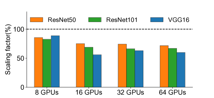
Figure 1. Scaling factor vs. number of servers involved.

2.2. What is the current scaling factor?

The first step is to understand the current scaling factor that can be achieved by an off-the-shelf distributed training framework like Horovod. We use the throughput of a single GPU (i.e., the number of images that can be processed by a GPU each second) as the base throughput $T$. We vary the number of servers in the experiments. For each case, we measure the total throughput that can be achieved by the servers and compute the scaling factor based on Equation 1. Figure 1 shows the scaling factor for each model under different numbers of servers. Remember that we use p3dn.24xlarge instances, each of which contains 8 GPUs. So the figure shows the scaling factor from 8 GPUs to 64 GPUs. The results indicate that the scaling factors for ResNet50, ResNet101 and VGG16 are 75.05%, 68.92%, and 55.99% for 2 servers, 74.24%, 66.28% and 63.01% for 4 servers, and 71.6%, 66.99% and 59.8% for 8 servers. ResNet50 achieves better scaling factors than ResNet101 and VGG16 as it has a relatively smaller model size to ease the communication burden. Nevertheless, for all the three models, Horovod cannot achieve a scaling factor of more than 76% on AWS.

These results confirm that the current off-the-shelf distributed training framework like Horovod cannot achieve linear scaling but with a significant gap.

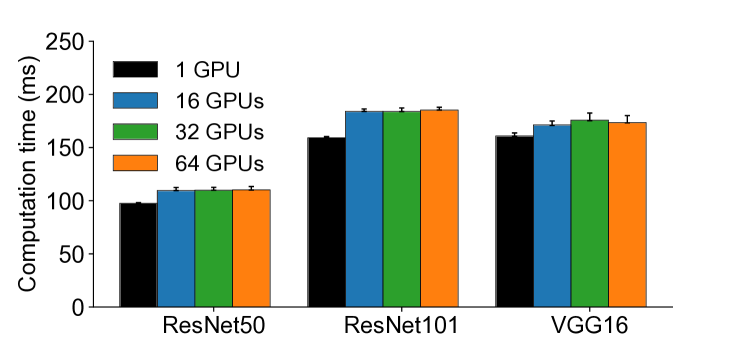
Figure 2. Computation time vs. number of servers.

2.3. Is computation the bottleneck?

Distributed training contains a computation component and a communication component. To figure out why linear scaling cannot be achieved, we start with the computation component. In the computation component, each worker feeds a batch of labeled images to the neural network model and computes the gradients locally. If the computation time for a worker to finish its batch increases with the number of workers, then the computation component would be the bottleneck of distributed training.

Figure 2 shows the computation time (for the forward and backward pass) for the three models with different number of workers. The computation time keeps almost the same, regardless of the number of workers. The time gap between single GPU and multiple GPUs comes mainly from two factors. First, the runtime for the backward pass in distributed training not only includes backward operations but also the all-reduce operations since they are asynchronous on GPU and overlapped. Whereas, for the single GPU case, there is no all-reduce operation. Second, Horovod injects a hook for each layer in the model during distributed training, which does not exist in single GPU training. However, even considering this computation time gap as an inevitable side effect, the scaling factor should still be bounded around 90% instead of the measured 56%-75%, because the measured computation time increases at most 15% in distributed training. Thus, we argue computation time difference here is not a factor for distributed training not able to scale linearly.

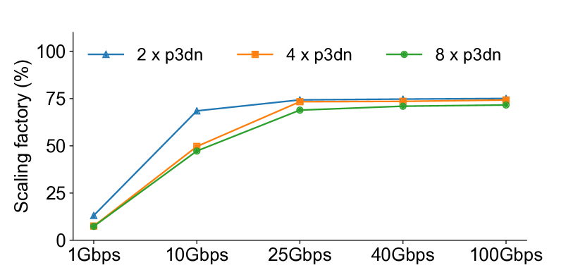
Figure 3. Scaling factor change with bandwidth (ResNet50).

2.4. Is network the bottleneck?

Now we turn to the communication component. Since the computation component takes the same amount of time regardless of the number of servers, then the only possibility is that the communication component is the bottleneck when the system scales out. To see whether this is the case, we first measure the scaling factor with different network bandwidths. As shown in Figure 3, the scaling factor for ResNet50 does increase when the network bandwidth increases. In the case of two servers, the scaling factor grows from 13% to 68% when the bandwidth increases from 1 Gbps to 10 Gbps. This is understandable as with higher bandwidth, it takes less time for the workers to exchange the same amount of data. The scaling factor is lower with more workers as they have more data to exchange, based on the all-reduce algorithm.

However, contrary to the common belief that the network is too slow to send the gradients, Figure 3 shows that the lines plateau after 25 Gbps. This means the system can not benefit from a faster network. To validate this, we measure the network utilization of the servers by recording real time network throughput. Figure 4 indicates that the servers do fully utilize the network at low bandwidth (e.g., 1 Gbps), but they only use a small fraction of the bandwidth at high bandwidth (e.g., 100 Gbps). This means merely adding bandwidth to make the network faster is not useful for improving scaling factor after a certain point.

(a) Network (Recv) utilization.

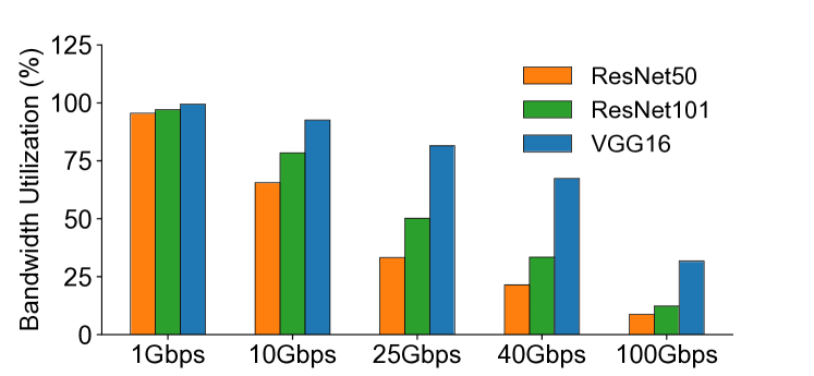
(b) Network (Send) utilization.

Figure 4. Network bandwidth utilization.

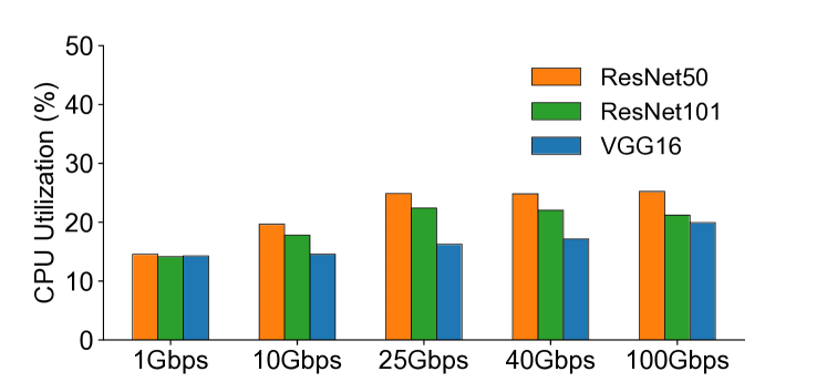
Figure 5. CPU utilization.

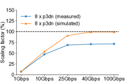
(a) ResNet50.

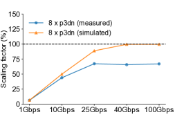
(b) ResNet101.

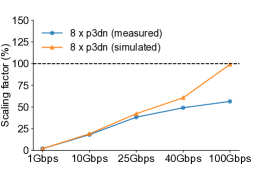
(c) VGG16.

Figure 6. Simulated scaling factor vs measured scaling factor in different bandwidth.

One possibility for low utilization at high bandwidth is that the CPU might be the bottleneck, as the experiments run Horovod over TCP and it is known that running TCP at high speed like 100 Gbps is CPU-intensive. However, the computation of distributed training is mostly done by GPUs, and most GPU instances are equipped with sufficient amount of CPUs (e.g., 96 vCPUs in a p3dn instance used by our experiments). Figure 5 shows the CPU utilizations while training three models on eight p3dn instances under five different network speeds. It confirms that the CPU utilization is low, and thus CPU is not the bottleneck for saturating 100 Gbps network bandwidth.

In conclusion, the measurement confirms that the communication component is the bottleneck. But contrary to the common belief, it is not because the network is too slow to send data. The root cause is the poor implementation of the network transport that cannot fully utilize the available bandwidth for the communication component.

3. What-If Analysis

Given the low network utilization, a natural question is what if the network can be fully utilized. In this section, we perform a what-if analysis to evaluate the scaling factor under full network utilization. Given the promise of many proposals on application-layer optimizations, we also use what-if analysis to show what additional improvements these proposals can bring if the network is fully utilized.

3.1. What if network can be fully utilized?

We first perform a what-if analysis to see what scaling factors can be achieved if the network is fully utilized. To do the what-if analysis, we need detailed logging information first, then perform simulation based on the timing logs. We take the white-box approach to directly add logging code to training scripts to retrieve detailed timing information for what-if analysis. Specifically, we add hooks for parameters in the model to get the gradient-computation-done time for different layers of the model.

For the simulation, we have two processes, backward process and all-reduce process. Two processes communicate through a message queue. The backward process simulates the backward computation which is based on the timing log of gradient-computation-done. The backward process does not request all-reduce process right after backward computation done for a certain layer. Instead, it buffers gradients of several layers for all-reduce. We use a heuristic buffering strategy, which refers to Horovod fusion buffer (sergeev2018horovod, ). Specifically, the backward process has a timeout window of 5 ms and a gradients buffer size of 64 MB for batching gradients for the all-reduce operations. Once the timeout criterion or buffer size limit is satisfied, it notifies the all-reduce process for all-reduce operation. The all-reduce process uses Reduce-scatter with Allgather procedures to complete all-reduce operation. The transition time is computed as $(2S(N-1)/N)/bw$, where $N$ is the number of workers/GPUs involved, $S$ is the size for all-reduce and $bw$ is the network bandwidth. The cost of vector additions is estimated as $(N-1)\times AddEst(S/N)$, where $AddEst(x)$ is the function for estimating the time of element-wise adding of two vectors in the size $x$. To fairly estimate the vector addition time cost, we first empirically evaluate time cost of vector-add with various vector sizes on V100 GPU, and then use linear interpolation to get $AddEst(x)$.

To get the scaling factor for a certain bandwidth and number of workers, we start backward process and all-reduce process at the same time for simulation. For each data batch, we denote the time for all-reduce process to complete as $t_{sync}$, and denote the time for backward computation $t_{back}$, thus we can get the overhead for all-reduce operation as $t_{overhead}=t_{sync}-t_{back}$. Then, we can use processing time of a batch data on single GPU, $t_{batch}$, to get the simulated scaling factor: $f_{sim}=t_{batch}/(t_{batch}+t_{overhead})$.

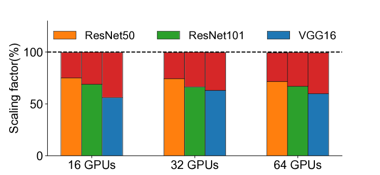
Figure 7. Simulated scaling factor under 100 Gbps network. Red parts denote the gap to simulated results.

Figure 6 shows the scaling factors of the three models under different network speeds assuming the network is fully utilized, and compares them with the scaling factors actually achieved by Horovod. We can see that under low network speeds (i.e., 1 Gbps and 10 Gbps), the two lines are very close. This confirms the results in Figure 4 that the network is fully utilized under low speeds, and also validates the correctness of the what-if simulator. Under high network speeds (i.e., after 25 Gbps), the two lines begin to diverge significantly. While the system can theoretically achieve close to 100% scaling factor under 100 Gbps for ResNet50, ResNet101 and VGG16, in practice it only achieves 75%, 67% and 60%, respectively.

We also use the what-if analysis to evaluate the scaling factors under different numbers of workers assuming that the network is fully utilized. The results are shown in Figure 7. Again, we see all of three models can achieve close to 100% scaling factors when the network is fully utilized even for 64 GPUs. Overall, the what-if analysis confirms that distributed training can benefit from high network bandwidth, moreover the scaling factor can be improved to near 100% if the network is fully utilized.

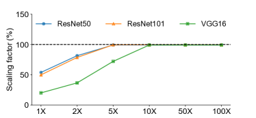
(a) Compression in 10Gbps network.

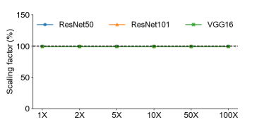
(b) Compression in 100Gbps network.

Figure 8. Simulated scaling factor under different compression ratio.

3.2. How useful are application-layer optimizations?

In this section our analysis targets a well-studied application-level optimization technique—gradient compression. We keep other simulation steps the same as we do in §3.1, but divide the time cost of gradients transmission by the compression ratio we choose. We use this setup for the simplicity. As one would imagine, the compression could possibly reduce the vector-add cost (e.g. half-precision vector-add, top-k percent gradients for all-reduce) to further boost the simulated scaling factor. But as shown in Figure 8, the simplified simulation is good enough to justify the claim we want to make, which is we probably would not need that high compression ratio as advocated in past works (lin2017deep, ; mishchenko2019distributed, ; lim20183lc, ). The compression ratio 10$\times$ is large enough for models like VGG16 to get scaling factor near 100% in 10 Gbps network, which is commonly available at cloud platform like AWS, GCloud and Azure. As a comparison, the results in 100 Gbps are also reported to indicate that compression is not that useful in high-speed networks, which is the typical network configuration for high-end GPU servers like aws-p3dn. In conclusion, gradient compression techniques are useful in low-speed networks, but it is not necessary to have a large compression ratio in contemporary network environments.

4. Discussion and Future Work

Rationale behind the findings. At first glance, our findings may be surprising, indicating that the scaling factor can be close to 100% if the network is fully utilized. These findings, however, are quite reasonable because of two important factors. First, the network runs at high speed. Under 100 Gbps, it only takes 7.8 ms, 13.6 ms and 42.2 ms to transmit all parameters of ResNet50, ResNet101 and VGG16, respectively. Second, there is a significant overlapping between computation and communication. The all-reduce for the last layer can start as soon as the backward process has computed the gradients of the last layer, without waiting for the entire backward process to finish. This overlap is critical. In conclusion, combining the efficient communication and the overlapping of computation and communication, the scaling factor can achieve near 100%.

Generality of the results. One essential question is how general are the results. The results are based on three models (ResNet50, ResNet101 and VGG16), one particular device (NVIDIA V100), and one training strategy (all-reduce). As part of our future work, we plan to expand the measurement and analysis to more models (e.g., RNN-like sequence models and BERT), more devices (different GPUs and other specialized processors), and more training strategies (e.g., parameter server and asynchronous training). While the actual numbers might differ, we expect that the conclusion would stay the same. i.e., because of high-speed networks and the intrinsic overlap between computation and communication, increasing the network utilization would result in almost linear scaling.

Trade-off of application-layer optimizations. The what-if analysis indicates that gradient compression in the application layer only provides meaningful improvements at low network bandwidths. We argue that it is not particularly useful for distributed training on the cloud or an on-premises cluster equipped with GPUs or TPUs. Those machines are typically connected with high-speed networks to fully utilize the processors. It does not make sense to build a cluster for distributed training with expensive specialized processors but a cheap, slow network.

The proper metric for scaling. We use throughput to compute the scaling factor. Another proper metric is to use the convergence time, i.e., the time to train a model to reach a certain accuracy threshold. Ideally, with $n$ servers, the convergence time should be cut by $n$ times (i.e., 100% scaling factor). This metric might be the most important metric cared by researchers and developers. We emphasize that network-layer optimizations provide consistent performance on both metrics, as it reduces the time to finish one iteration without changing the number of iterations needed to reach a certain accuracy. Also, network optimizations are orthogonal to other techniques to accelerate the training process (you2018imagenet, ). Gradient compression, on the other hand, loses gradient information due to lossy compression, and can prolong the convergence time, hurt the accuracy, and even end up not being able to converge.

What-if analysis for other approaches. Besides gradient compression, there are other application-layer and system-layer optimizations. For example, ByteScheduler (peng2019generic, ) orders the gradient transmission of different layers to better overlap with forward computation; and SwitchML (sapio2019scaling, ) uses a programmable switch to aggregate gradients and reduce the communication size. These proposals all suggest significant reduction on the training time. However, they are all compared to an off-the-shelf distributed training framework like Horovod, which has a poor network transport implementation. It would be interesting to apply the what-if analysis to evaluate what additional improvements they can provide if the network can be highly utilized.

High-performance network transport for distributed training. There is always an arms race between compute and network. When compute is improved, network becomes the bottleneck. Our findings indicate that for today’s distributed training systems, the network speed is not a problem, but the network transport implementation for the communication component is. Compared to application-layer optimizations, e.g. gradient compression, network-layer optimizations do not trade training time off against model accuracy, and should be the first-order optimizations. As such, our results are a call for the network community to develop high-performance network transport to fully utilize modern high-speed networks and to achieve linear scale-out. Recently, AWS has provided Elastic Fabric Adapter (EFA) as an efficient network interface to bypass OS kernel for high-performance communication (EFA, ), and achieved some encouraging scalability results by carefully tuning the training process (EFAtraining, ). Developing high-performance network transport with kernel-bypass technologies in the context of distributed training is an interesting direction of future work.

Acknowledgments. We thank the anonymous reviewers for their valuable feedback. This work is supported in part by NSF grants CRII-1755646, CNS-1813487 and CCF-1918757, and an AWS Machine Learning Research Award. RA would like to acknowledge support from NSF under the BIGDATA awards IIS-1546482 and IIS-1838139, and NSF CAREER award IIS-1943251.

References

- (1) “AI and Compute.” https://openai.com/blog/ai-and-compute/.
- (2) “GPUs Power Five of World’s Top Seven Supercomputers.” https://www.hpcwire.com/2018/06/25/gpus-power-five-of-worlds-top-seven-supercomputers/.
- (3) “Cloud TPU.” https://cloud.google.com/tpu/.
- (4) Y. Peng, Y. Zhu, Y. Chen, Y. Bao, B. Yi, C. Lan, C. Wu, and C. Guo, “A generic communication scheduler for distributed dnn training acceleration,” in ACM SOSP, 2019.
- (5) Y. Lin, S. Han, H. Mao, Y. Wang, and W. J. Dally, “Deep gradient compression: Reducing the communication bandwidth for distributed training,” arXiv preprint arXiv:1712.01887, 2017.
- (6) A. Sapio, M. Canini, C.-Y. Ho, J. Nelson, P. Kalnis, C. Kim, A. Krishnamurthy, M. Moshref, D. R. Ports, and P. Richtárik, “Scaling distributed machine learning with in-network aggregation,” arXiv preprint arXiv:1903.06701, 2019.
- (7) W. Wen, C. Xu, F. Yan, C. Wu, Y. Wang, Y. Chen, and H. Li, “Terngrad: Ternary gradients to reduce communication in distributed deep learning,” in NeurIPS, 2017.
- (8) D. Narayanan, A. Harlap, A. Phanishayee, V. Seshadri, N. R. Devanur, G. R. Ganger, P. B. Gibbons, and M. Zaharia, “Pipedream: generalized pipeline parallelism for dnn training,” in ACM SOSP, 2019.
- (9) A. F. Aji and K. Heafield, “Sparse communication for distributed gradient descent,” in Proceedings of the 2017 Conference on Empirical Methods in Natural Language Processing, Association for Computational Linguistics, 2017.
- (10) D. Alistarh, J. Li, R. Tomioka, and M. Vojnovic, “Qsgd: Randomized quantization for communication-optimal stochastic gradient descent,” arXiv preprint arXiv:1610.02132, 2016.
- (11) C.-Y. Chen, J. Choi, D. Brand, A. Agrawal, W. Zhang, and K. Gopalakrishnan, “Adacomp: Adaptive residual gradient compression for data-parallel distributed training,” in Thirty-Second AAAI Conference on Artificial Intelligence, 2018.
- (12) J. Konečnỳ, H. B. McMahan, F. X. Yu, P. Richtárik, A. T. Suresh, and D. Bacon, “Federated learning: Strategies for improving communication efficiency,” arXiv preprint arXiv:1610.05492, 2016.
- (13) J. Wangni, J. Wang, J. Liu, and T. Zhang, “Gradient sparsification for communication-efficient distributed optimization,” in Advances in Neural Information Processing Systems, 2018.
- (14) H. Wang, S. Sievert, S. Liu, Z. Charles, D. Papailiopoulos, and S. Wright, “Atomo: Communication-efficient learning via atomic sparsification,” in Advances in Neural Information Processing Systems, 2018.
- (15) N. Ivkin, D. Rothchild, E. Ullah, I. Stoica, and R. Arora, “Communication-efficient distributed SGD with sketching,” in Advances in Neural Information Processing Systems, 2019.
- (16) D. Rothchild, A. Panda, E. Ullah, N. Ivkin, J. Gonzalez, I. Stoica, and R. Arora, “FetchSGD: Communication-efficient federated learning with sketching,” in International conference on machine learning (ICML), 2020.
- (17) F. Seide, H. Fu, J. Droppo, G. Li, and D. Yu, “1-bit stochastic gradient descent and its application to data-parallel distributed training of speech dnns,” in Fifteenth Annual Conference of the International Speech Communication Association, 2014.
- (18) H. Lim, D. G. Andersen, and M. Kaminsky, “3lc: Lightweight and effective traffic compression for distributed machine learning,” arXiv preprint arXiv:1802.07389, 2018.
- (19) A. Sergeev and M. Del Balso, “Horovod: fast and easy distributed deep learning in tensorflow,” arXiv preprint arXiv:1802.05799, 2018.
- (20) “TensorFlow.” https://www.tensorflow.org/.
- (21) “PyTorch.” https://pytorch.org/.
- (22) “MXNet.” https://mxnet.apache.org/.
- (23) K. He, X. Zhang, S. Ren, and J. Sun, “Deep residual learning for image recognition,” in IEEE CVPR, 2016.
- (24) K. Simonyan and A. Zisserman, “Very deep convolutional networks for large-scale image recognition,” arXiv preprint arXiv:1409.1556, 2014.
- (25) J. Deng, W. Dong, R. Socher, L.-J. Li, K. Li, and L. Fei-Fei, “Imagenet: A large-scale hierarchical image database,” in IEEE CVPR, 2009.
- (26) K. Mishchenko, E. Gorbunov, M. Takáč, and P. Richtárik, “Distributed learning with compressed gradient differences,” arXiv preprint arXiv:1901.09269, 2019.
- (27) Y. You, Z. Zhang, C.-J. Hsieh, J. Demmel, and K. Keutzer, “Imagenet training in minutes,” in Proceedings of the 47th International Conference on Parallel Processing, 2018.
- (28) “Optimizing deep learning on P3 and P3dn with EFA.” https://aws.amazon.com/blogs/compute/optimizing-deep-learning-on-p3-and-p3dn-with-efa/.
- (29) “Amazon Web Services achieves fastest training times for BERT and Mask R-CNN.” https://aws.amazon.com/blogs/machine-learning/amazon-web-services-achieves-fastest-training-times-for-bert-and-mask-r-cnn/.