Nearly Optimal Robust Method for Convex Compositional Problems with Heavy-Tailed Noise

Abstract

In this paper, we propose robust stochastic algorithms for solving convex compositional problems of the form $f(\mathrm{E}_{\xi}g(\cdot;\xi))+r(\cdot)$ by establishing sub-Gaussian confidence bounds under weak assumptions about the tails of noise distribution, i.e., heavy-tailed noise with bounded second-order moments. One can achieve this goal by using an existing boosting strategy that boosts a low probability convergence result into a high probability result. However, piecing together existing results for solving compositional problems suffers from several drawbacks: (i) the boosting technique requires strong convexity of the objective; (ii) it requires a separate algorithm to handle non-smooth $r$; (iii) it also suffers from an additional polylogarithmic factor of the condition number. To address these issues, we directly develop a single-trial stochastic algorithm for minimizing optimal strongly convex compositional objectives, which has a nearly optimal high probability convergence result matching the lower bound of stochastic strongly convex optimization up to a logarithmic factor. To the best of our knowledge, this is the first work that establishes nearly optimal sub-Gaussian confidence bounds for compositional problems under heavy-tailed assumptions.

1 Introduction

In this paper, we consider the following stochastic compositional problem:

$$\min_{\mathbf{w}\in\mathbb{R}^{d}}F(\mathbf{w}):=f(\mathrm{E}_{\xi}[g(\mathbf{w};\xi)])+r(\mathbf{w}),$$ (1)

where $\xi$ is a random variable, $f:\mathbb{R}^{p}\rightarrow\mathbb{R}$ is a smooth and Lipschitz continuous function and $r(\cdot)$ is convex and lower-semicontinuous. Denote by $g(\mathbf{w})=\mathrm{E}_{\xi}[g(\mathbf{w};\xi)]$. We focus on a family of problems where $f(g(\mathbf{w}))$ is smooth convex but $F(\mathbf{w})$ is optimal strongly convex Liu and Wright (2015). We aim to develop efficient stochastic algorithms enjoying a sub-Gaussian confidence bound $\Pr(F(\bar{\mathbf{w}})-\min_{\mathbf{w}}F(\mathbf{w})\leq\epsilon)\geq 1-\delta$, under weak assumptions about the random function $g(\mathbf{w};\xi)$ and its Jacobian.

The above problem has a broad range of applications in machine learning, operation research, etc Wang et al. (2017a). Although a number of papers have proposed stochastic algorithms for solving the stochastic compositional problem (1), they are mostly low probability convergence results. To the best of our knowledge, all of the existing results of (1) are expectational convergence results in the form of $\mathrm{E}[F(\bar{\mathbf{w}})-\min_{\mathbf{w}}F(\mathbf{w})]\leq\epsilon^{\prime}$ with a polynomial sample complexity denoted by $\mathcal{C}(1/\epsilon^{\prime})$ . By Markov inequality, this directly implies a low probability convergence result $\Pr(F(\bar{\mathbf{w}})-\min_{\mathbf{w}}F(\mathbf{w})\leq\epsilon^{\prime}/\delta)\geq 1-\delta$ for a constant $\delta$. Hence, in order to guarantee $\Pr(F(\bar{\mathbf{w}})-\min_{\mathbf{w}}F(\mathbf{w})\leq\epsilon)\geq 1-\delta$ for a small $\epsilon$, the sample complexity will be amplified by an undesired polynomial factor of $1/\delta$, i.e., $\mathcal{C}(1/(\delta\epsilon))$. In this paper, we are interested in achieving a high probability convergence result with a logarithmic dependence on $1/\delta$, which is also known as sub-Gaussian confidence bound.

High probability convergence results have been established for many stochastic convex optimization problems in the literature Nemirovski et al. (2009); Hazan and Kale (2011); Rakhlin et al. (2012); Xu et al. (2016); Ghadimi and Lan (2013). However, most of them are derived under bounded assumption or sub-Gaussian assumptions about stochastic functions. In practice, these assumptions could fail when data suffer from dramatic noise. For the robust learning problem considered later on (in the supplement), the individual loss $g(\mathbf{w};\xi)$ and its gradient $\nabla g(\mathbf{w};\xi)$ could be unbounded or follow a heavy-tailed distribution due to outliers or adversarial attack. In this paper, we avoid making such restrictive assumptions by imposing the following weak assumptions about the noisy function value and the noisy Jacobian of $g(\mathbf{w})$:

$$\mathrm{E}[\|\nabla g(\mathbf{w};\xi)\|^{2}]\leq C_{g}^{2},\quad\mathrm{E}[\|\nabla g(\mathbf{w};\xi)-\nabla g(\mathbf{w})\|^{2}]\leq\sigma_{1}^{2},\quad\mathrm{E}[\|g(\mathbf{w};\xi)-g(\mathbf{w})\|^{2}]\leq\sigma_{0}^{2},$$ (2)

where $\|\cdot\|$ denotes the Euclidean norm of a vector or the spectral norm of a matrix.

Recently, Davis et al. Davis et al. (2019) proposed a generic boosting technique that can boost a low probability convergence result into a high probability convergence result for minimizing a strongly convex objective function. It comes at a cost increase that depends on a polylogarithmic factor of the condition number. Combining this boosting technique with existing stochastic algorithms for (1) (e.g., Wang et al. (2017a)) can provide a solution to achieving a high probability convergence result. However, such a “lazy" solution is not necessarily the best solution. First, the boosting technique requires strong convexity of the objective; Second, it requires a separate algorithm to handle non-smooth $r$; Third, it also suffers from an additional polylogarithmic factor of the condition number. We make the following contributions to address these issues.

• First, we propose a simple robust algorithm for optimal strongly convex function $F(\mathbf{w})$ by using robust mean estimation technique. It enjoys a sample complexity in the order of $O(\frac{\log(\kappa/\delta)}{\mu^{2}\epsilon})$ for achieving $\Pr(F(\bar{\mathbf{w}})-\min_{\mathbf{w}}F(\mathbf{w})\geq\epsilon)\leq 1-\delta$, where $\kappa$ is the condition number of the problem.

• Second, we develop an improved stochastic algorithm by combining robust mean estimation technique and a reference truncation technique. It enjoys a sample complexity in the order of $O(\frac{\log^{2}(\log(1/\epsilon)/\delta)}{\mu\epsilon})$ for achieving $\Pr(F(\bar{\mathbf{w}})-\min_{\mathbf{w}}F(\mathbf{w})\geq\epsilon)\leq 1-\delta$ for $\mu$-optimal strongly convex function $F(\mathbf{w})$. This sample complexity matches the lower bound of stochastic strongly convex optimization not only in terms of $\epsilon$ but also in terms of $\mu$ up to a marginal logarithmic factor.

To the best of our knowledge, this is the first work that establishes nearly optimal sub-Gaussian confidence bounds for compositional problems under heavy-tailed assumptions.

2 Related Work

Stochastic Compositional Problems. Research on stochastic compositional problems dates back to 70s by Ermoliev Ermoliev (1976). The first non-asymptotic convergence analysis was given by Wang et al. in 2014 Wang et al. (2017a). They considered a broader family of problems in the form of $\mathrm{E}_{v}[f_{v}(\mathrm{E}_{\xi}g_{\xi}(\mathbf{w}))]$, where both $f$ and $g$ are random functions. Under the same conditions of this paper and Lipschitz continuity and bounded second-order moment of $\nabla f_{v}(\cdot)$, the authors established a convergence rate of $O(1/T^{1/4})$ with $T$ iterations of updates for a general convex objective in terms of the objective gap, and $O(1/(\mu^{8/3}T^{2/3}))$ for $\mu$-strongly convex objective in terms of distance of solution to the optimal set. Applying to our problem, it implies a sample complexity of $O(1/(\mu^{4}\epsilon^{1.5}))$ for making the objective gap $\epsilon$ small. When the objective function is smooth, the authors also developed a faster convergence rate in order of $O(1/(\mu^{14/5}T^{4/5}))$ under a stronger assumption about $\nabla g_{\xi}(\mathbf{w})$, i.e., the fourth-order moment is bounded. They also consider non-convex smooth objectives, which is out of scope of this paper.

A series of extensions and improvements were made in later works. Wang et al. Wang et al. (2017b) extended their algorithms to solving additive compositional problem of the form $\mathrm{E}_{v}[f_{v}(\mathrm{E}_{\xi}g_{\xi}(\mathbf{w}))]+r(\mathbf{w})$ where $r$ is a non-smooth convex regularizer. They improved the rates to $O(1/T^{2/7})$ for a general convex objective and $O(1/T^{4/5})$ for an optimal strongly convex objective. They also achieved a sample complexity of $O(1/\epsilon)$ when $f$ is linear or $g$ is linear. However, in terms of assumptions on random function $g_{\xi}(\mathbf{w})$ they simply assume that its gradient is bounded. In contrast, this paper considered that $f$ is deterministic and established fast rates as good as $O(1/\epsilon)$ under much weaker assumptions. Yang et al. Yang et al. (2019) considered multi-level stochastic compositional problem under similar bounded moment assumptions as made in Wang et al. (2017a) and established generic convergence rate dependent on the stochasticity level. Wang and Liu Wang and Liu (2016) also considered Markov noise in estimating $g$, $\nabla g$ and $\nabla f$, and established a rate of $O(1/T^{1/6})$ for general convex objectives under bounded noise assumptions.

Improved rates were established by using variance reduction techniques (e.g., SVRG Johnson and Zhang (2013), SCCG Lei and Jordan ) for finite-sum problems Lian et al. (2017); Lin et al. (2018); Liu et al. (2019); Huo et al. (2018); Liu et al. (2018); Zhang and Xiao (2019b, a); Yu and Huang (2017). These works established linear convergence for finite-sum problems with strongly convex objectives and improved sub-linear convergence for general objectives. In these works, they simply assume the inner function $g_{\xi}(\cdot)$ has bounded and Lipschitz continuous gradient. Some of these works also considered online problems without a finite-sum structure, and a sample complexity in the order of $O(1/\epsilon)$ was also achieved in some of these works for (optimal) strongly convex objectives. For example, Liu et al. Liu et al. (2018) considered $\mathrm{E}_{v}[f_{v}(\mathrm{E}_{\xi}g_{\xi}(\mathbf{w}))]$ and their algorithms enjoy a sample complexity of $O(1/(\mu^{2}\epsilon))$ for finding a solution $\bar{\mathbf{x}}$ such that $\mathrm{E}[\|\bar{\mathbf{x}}-\mathbf{x}_{*}\|^{2}]\leq\epsilon$. Zhang & Xiao Zhang and Xiao (2019a) considered the same objective $f(\mathrm{E}_{\xi}g(\cdot;\xi))+r(\cdot)$ as in this work and and their algorithms enjoy a sample complexity of $O(\log(1/\epsilon)/(\mu\epsilon))$ for finding a solution $\bar{\mathbf{x}}$ such that $\mathrm{E}[F(\bar{\mathbf{x}})-F(\mathbf{x}_{*})]\leq\epsilon$ when $F$ is $\mu$-optimal strongly convex. Nevertheless, these works require each random function $g_{\xi}(\cdot)$ to be smooth or at least smooth in expectation, i.e., $\mathrm{E}_{\xi}\|\nabla g_{\xi}(\mathbf{w}_{1})-\nabla g_{\xi}(\mathbf{w}_{2})\|^{2}\leq O(\|\mathbf{w}_{1}-\mathbf{w}_{2}\|^{2})$. In contrast, we avoid making this assumption and enjoy a similar sample complexity in the order of $O(\log(\log(1/\epsilon))/(\mu\epsilon))$ with high probability.

Robust Stochastic Methods. Many studies have established sub-Gaussian convergence bounds for stochastic convex optimization Nemirovski et al. (2009); Hazan and Kale (2011); Rakhlin et al. (2012); Xu et al. (2016); Ghadimi and Lan (2013). But most of them assume the noise is light-tailed (e.g., bounded or sub-Gaussian). Recently, Davis et al. Davis et al. (2019) proposed a generic boosting technique to boost any low convergence results that can be achieved under heavy-tailed noise into high probability convergence for strongly convex objectives. It is unclear how strong convexity can be alleviated into optimal strong convexity condition of the objective, which captures a much broader family of problems. Their algorithm is built on the proximal point method and robust distance estimation technique Hsu and Sabato (2016). Nazin et al. Nazin et al. (2019) proposed robust mirror descent method for solving stochastic convex optimization problems based on truncating stochastic gradient. They also considered optimal strongly convex objective and established a fast rate of $O(\log(\log(\kappa)/\delta)/(\mu\epsilon))$. However, we notice that they assumed the optimal set is in the interior of the constrained domain. We avoid such condition in order to capture a broader family of problems. There also exists many studies focusing on sub-Gaussian confidence bounds for empirical loss minimization and bandits problems under heavy-tailed assumption Hsu and Sabato (2014, 2016); Audibert and Catoni (2011); Xu et al. (2019); Zhang and Zhou ; Lu et al. (2019); Bubeck et al. (2013), which is out of scope of this work.

3 Preliminaries

We denote by $\|\cdot\|$ the Euclidean norm of a vector or the Frobenius norm of a matrix. Define $\mathcal{B}(\mathbf{c},r)=\{\mathbf{x}\in\mathbb{R}^{p}:\|\mathbf{x}-\mathbf{c}\|\leq r\}$ an Euclidean ball centered at $\mathbf{c}$ with a radius $r$. A function $h(\mathbf{w})$ is $\mu$-strongly convex if for any $\mathbf{w},\mathbf{w}^{\prime}$ it holds $h(\mathbf{w})\geq h(\mathbf{w}^{\prime})+\partial h(\mathbf{w}^{\prime})(\mathbf{w}-\mathbf{w}^{\prime})+\frac{\mu}{2}\|\mathbf{w}-\mathbf{w}^{\prime}\|^{2}$. A function $h(\mathbf{w})$ is said to be $\mu$-optimal strongly convex if for any $\mathbf{w}$ it holds $h(\mathbf{w})-\min_{\mathbf{w}}h(\mathbf{w})\geq\frac{\mu}{2}\|\mathbf{w}-\mathbf{w}_{*}\|^{2}$, where $\mathbf{w}_{*}$ is an optimal solution (not necessarily unique) that is closest to $\mathbf{w}$. This condition is also known as the quadratic growth condition in some literature Xu et al. (2016). It is much weaker than the strong convexity condition.

Including the assumptions in (2), we make the following assumptions throughout the paper.

Assumption 1.

Let $C_{f}$, $L_{f}$, $C_{g}$, $L_{g}$, $\sigma_{1}$ and $\sigma_{0}$ be positive scalars.

• (i): $f(\cdot)$ is $C_{f}$-Lipschitz continuous and has $L_{f}$-Lipschitz continuous gradients.

• (ii): $g(\cdot)$ has $L_{g}$-Lipschitz continuous gradient.

• (iii): $f(g(\cdot))$ and $r(\cdot)$ are convex functions, $F(\mathbf{w})$ is $\mu$-optimal strongly convex.

• (iv): Regarding the random function $g(\mathbf{w};\xi)$, we have

  $$\mathrm{E}[\|\nabla g(\mathbf{w};\xi)\|^{2}]\leq C_{g}^{2},\quad\mathrm{E}[\|\nabla g(\mathbf{w};\xi)-\nabla g(\mathbf{w})\|^{2}]\leq\sigma_{1}^{2},\quad\mathrm{E}[\|g(\mathbf{w};\xi)-g(\mathbf{w})\|^{2}]\leq\sigma_{0}^{2}.$$

Remark 1.

The first two assumptions are used to ensure that $f(g(\mathbf{w}))$ is a $L$-smooth function with $L=(C_{f}L_{g}+C_{g}^{2}L_{g})$, which were also imposed in Wang et al. (2017a). However, the difference from previous works lies at the third assumption regarding the random function $g(\cdot;\xi)$. Many studies impose much stronger assumptions than ours. For example, Wang et al. Wang et al. (2017a) assumed that the fourth order moments $\mathrm{E}\|\nabla g(\mathbf{w};\xi)\|^{4}$ is bounded in order to derive a faster rate for strongly convex problems in the order of $O(1/\epsilon^{5/4})$. Wang et al. Wang et al. (2017b) simply assume that $\|\nabla g(\mathbf{w};\xi)\|$ is bounded. Zhang & Xiao Zhang and Xiao (2019a) assumed that $g(\mathbf{w};\xi)$ has bounded and Lipschitz continuous gradient. Please also note that $\mathrm{E}\|\nabla g(\mathbf{w};\xi)\|^{2}\leq C_{g}^{2}$ indicates that $g(\mathbf{w})$ is $C_{g}$-Lipschitz continuous. Below, we let $\kappa=L/\mu$ denote the condition number of the problem.

An ingredient of the proposed robust stochastic algorithm is the robust mean estimator, which has been studied in many previous works Nemirovsky A.S. and IUdin (c1983.); Hsu and Sabato (2016). Given a set of $n$ i.i.d random variables $X_{1},\ldots,X_{n}$ from the same distribution with a mean $\mu$ and finite variance $\sigma^{2}$, the problem is to obtain a robust mean estimator $\bar{\mu}$ with a sub-Gaussian confidence bound. Depending on whether the random variable is a scalar or a vector, we can use different approaches for computing the robust mean estimator. If $X_{i}\in\mathbb{R}$, we can use the simple median-of-means (MoM) estimator Nemirovsky A.S. and IUdin (c1983.); otherwise we can use the robust distance approximation method proposed in Hsu and Sabato (2016). We present both methods in Algorithm 1 and summarize their key properties below.

Lemma 1.

Given $n$ i.i.d. random variables $X_{1},...,X_{n}$ with mean $\mu$ and finite variance $\sigma^{2}$, let $\delta\in(0,1)$. If $X_{i}\in\mathbb{R}$, then Algorithm 1 with $m=\frac{n}{8\log(1/\delta)}$ and $k=8\log(1/\delta)$ guarantees that with probability at least $1-\delta$, we have $(\bar{\mu}-\mu)^{2}\leq\frac{32\sigma^{2}\log(1/\delta)}{n}$. If $X_{i}\in\mathbb{R}^{p}$, then Algorithm 1 with $m=\frac{n}{18\log(1/\delta)}$ and $k=18\log(1/\delta)$ guarantees that with probability at least $1-\delta$, we have $\|\bar{\bm{\mu}}-\bm{\mu}\|^{2}\leq\frac{486\sigma^{2}\log(1/\delta)}{n}$.

Algorithm 1 Robust Mean Estimator: RME($\{X_{1},\ldots,X_{n}\}$)

1:  Initialize $m$ and $k$ such that $mk=n$

2:  Compute $\bar{\mu}_{1}=\frac{1}{m}\sum_{i=1}^{m}X_{i},\ldots,\bar{\mu}_{k}=,\frac{1}{m}\sum_{i=(k-1)m+1}^{km}X_{i}$

3:  if $X_{i}\in\mathbb{R}$ then

4:     return $\bar{\mu}=\text{median}(\bar{\mu}_{1},\ldots,\bar{\mu}_{k})$

5:  else

6:     Define $\mathcal{X}=\{\bar{\mu}_{1},\ldots,\bar{\mu}_{k}\}$

7:     For each $i=1,\ldots,k$, compute $r_{i}=\min\{r\geq 0:|\mathcal{B}(\bar{\mu}_{i},r)\cap\mathcal{X}|\geq k/2\}$

8:     return $\bar{\mu}=\bar{\mu}_{i_{*}}$ where $i_{*}=\arg\min_{i\in\{1,\ldots,k\}}r_{i}$

9:  end if

4 A Baseline: From Low Probability to High Probability Convergence

In this section, we will present a logically simple solution to achieving a sub-Gaussian confidence bound under Assumption 1. In particular, we will first present an algorithm with an expectational convergence, and then boost it directly into high probability convergence by using robust mean estimators.

We describe the basic algorithm in Algorithm 2, which is referred to as mini-batch stochastic compositional gradient (MSCG) method. The key update in Step 5 mimics the well-known stochastic proximal gradient update except that the gradient estimator computed by $\mathbf{z}_{t+1}^{\top}f(\mathbf{y}_{t+1})$ is a biased stochastic gradient of $f(g(\mathbf{w}))$ at $\mathbf{w}_{t}$. In order to control the error of the gradient estimator, we use a mini-batch of data to compute an estimation of $g(\mathbf{w}_{t})$ and $\nabla g(\mathbf{w}_{t})$ by $\mathbf{y}_{t+1}$ and $\mathbf{z}_{t+1}$, respectively. The following lemma summarizes the convergence bound of MSCG.

Algorithm 2 MSCG$(\mathbf{w}_{0},\eta,T,\{m_{t}\})$

1:  for $t=0,...,T$ do

2:     Sample random samples $\mathcal{S}_{1},\mathcal{S}_{2}$ of size $m_{t}$

3:     (non-robust option) $\mathbf{y}_{t+1}=\frac{1}{m_{t}}\sum_{\xi\in\mathcal{S}_{1}}g(\mathbf{w}_{t};\xi)$ and $\mathbf{z}_{t+1}=\frac{1}{m_{t}}\sum_{\xi\in\mathcal{S}_{2}}\nabla g(\mathbf{w};\xi)$

4:     (robust option): $\mathbf{y}_{t+1}=\text{RME}(\{g(\mathbf{w}_{t};\xi),\xi\in\mathcal{S}_{1}\})$ and $\mathbf{z}_{t+1}=\text{RME}(\{\nabla g(\mathbf{w}_{t};\xi),\xi\in\mathcal{S}_{2}\})$

5:     $\mathbf{w}_{t+1}=\arg\min_{\mathbf{w}}\mathbf{z}_{t+1}^{\top}\nabla f(\mathbf{y}_{t+1})\mathbf{w}+\frac{1}{2\eta_{t}}\|\mathbf{w}-\mathbf{w}_{t}\|^{2}+r(\mathbf{w})$

6:  end for

7:  Output: $\widehat{\mathbf{w}}_{T}=\mathcal{O}(\mathbf{w}_{1},...,\mathbf{w}_{T})$

Algorithm 3 RMSCG

  Initialize $\mathbf{w}_{0},\eta,m_{1},T$

  for $k=1,...,K$ do

     $\mathbf{w}_{k}=$ MSCG$(\mathbf{w}_{k-1},\eta,T,m_{k})$

     Update $m_{k+1}=2m_{k}$

  end for

Lemma 2.

Suppose Assumption 1 holds. Let $F(\mathbf{w}_{0})-F(\mathbf{w}_{*})\leq\epsilon_{0}$. For Algorithm 2 with non-robust option and $\eta\leq\frac{1}{2L},\widehat{\mathbf{w}}_{T}=\frac{1}{T}\sum_{t=1}^{T}\mathbf{w}_{t}$, we have

$$\mathrm{E}[F(\widehat{\mathbf{w}}_{T})-F(\mathbf{w}_{*})]\leq\frac{\epsilon_{0}}{T}+\frac{1}{T}\sum_{t=0}^{T-1}\frac{4\eta(C_{f}^{2}\sigma_{1}^{2}+C_{g}^{2}L_{f}^{2}\sigma_{0}^{2})+2L_{f}^{2}C_{g}^{2}\sigma_{0}^{2}/\mu}{m_{t}}+\frac{\|\mathbf{w}_{0}-\mathbf{w}_{*}\|^{2}}{\eta T}.$$

Remark: By setting $m_{t}\propto(t+1)/\mu$, the above result implies $\mathrm{E}[F(\widehat{\mathbf{w}}_{T})-F(\mathbf{w}_{*})]\leq O(\frac{\log T}{T})$, which yields a sample complexity of $\sum_{t=1}^{T}m_{t}=\widetilde{O}(\frac{1}{\mu\epsilon^{2}})$ in order to have $\mathrm{E}[F(\widehat{\mathbf{w}}_{T})-F(\mathbf{w}_{*})]\leq\epsilon$.

Nevertheless, the above result can be improved by using the restarting trick. The algorithm is presented in Algorithm 3. Its convergence is summarized below.

Theorem 1.

Suppose Assumption 1 holds. Let $F(\mathbf{w}_{0})-F(\mathbf{w}_{*})\leq\epsilon_{0}$ and $\epsilon_{k}=\epsilon_{0}/2^{k}$. For Algorithm 3 with non-robust option, let $\eta\leq\frac{1}{2L}$, $T=4/(\mu\eta)$, $m_{k}=4(\mu\eta C_{f}^{2}\sigma_{1}^{2}+\mu\eta C_{g}^{2}L_{f}^{2}\sigma_{0}^{2}+C_{g}^{2}L_{f}^{2}\sigma_{0}^{2})/(\mu\epsilon_{k-1})$ and $\widehat{\mathbf{w}}_{T}=\sum_{t=1}^{T}\mathbf{w}_{t}/T$. The sample complexity for achieving $\mathrm{E}[F(\widehat{\mathbf{w}}_{T})-F(\mathbf{w}_{*})]\leq\epsilon$ is given by $m_{tot}=\tilde{O}(\frac{1}{\mu^{2}\epsilon})$.

Remark: We make a comparison with the result established in Wang et al. (2017a) under the same condition of Theorem 1. They proved a result for $\mathrm{E}[\|\mathbf{w}_{T}-\mathbf{w}_{*}\|^{2}]\leq\epsilon$ with a sample complexity of $O(\frac{1}{\mu^{3}\epsilon^{3/2}})$. When $r=0$, their result together with smoothness of $F$ implies that their algorithm has a sample complexity of $O(\frac{1}{\mu^{4}\epsilon^{3/2}})$ for achieving $\mathrm{E}[F(\mathbf{w})-F(\mathbf{w}_{*})]\leq\epsilon$. It is clear that our result in Theorem 1 is much better.

Next, we discuss how to boost the expectational convergence result into a high probability result without using the complicated boosting technique introduced by Davis et al. (2019). To this end, we present the following lemma for explaining the robust algorithms.

Lemma 3.

Suppose Assumption 1 holds. Let $\eta_{t}\leq\frac{1}{2L}$. After running $T$ iterations of Algorithm 2, we have

$$\frac{1}{T}\sum_{t=0}^{T-1}(F(\mathbf{w}_{t+1})-F(\mathbf{w}_{*}))\leq \frac{\|\mathbf{w}_{*}-\mathbf{w}_{0}\|^{2}}{2\eta T}+\frac{\eta}{T}\underbrace{\sum_{t=0}^{T-1}\|\nabla g(\mathbf{w}_{t})^{\top}\nabla f(g(\mathbf{w}_{t}))-\mathbf{z}_{t+1}^{\top}\nabla f(\mathbf{y}_{t+1})\|^{2}}_{A}$$

$$+\frac{1}{T}\underbrace{\sum_{t=0}^{T-1}\langle\nabla g(\mathbf{w}_{t})^{\top}\nabla f(g(\mathbf{w}_{t}))-\mathbf{z}_{t+1}^{\top}\nabla f(\mathbf{y}_{t+1}),\mathbf{w}_{t}-\mathbf{w}_{*}\rangle}_{B}$$ (3)

The first term in the upper bound can be handled by optimal strongly convexity by setting $\mathbf{w}_{*}$ as the closest optimal solution to $\mathbf{w}_{0}$ to build a recursion, i.e., $\|\mathbf{w}-\mathbf{w}_{*}\|^{2}\leq\frac{2}{\mu}(F(\mathbf{w}_{0})-F(\mathbf{w}_{*}))$. The challenge lies at bounding the second term $A$ and the third term $B$ with sub-Gaussian confidence bound. Let us consider how to bound $A$ with high probability. In order to do so, we decompose $A,B$ into two terms:

$$A/2\leq$$

$$\underbrace{\sum_{t=0}^{T-1}\|\nabla g(\mathbf{w}_{t})^{\top}\nabla f(g(\mathbf{w}_{t}))-\nabla g(\mathbf{w}_{t})^{\top}\nabla f(\mathbf{y}_{t+1})\|^{2}}_{A_{1}}+\underbrace{\sum_{t=0}^{T-1}\|\nabla g(\mathbf{w}_{t})^{\top}\nabla f(\mathbf{y}_{t+1})-\mathbf{z}_{t+1}^{\top}\nabla f(\mathbf{y}_{t+1})\|^{2}}_{A_{2}}$$

$$B\leq\underbrace{\sum_{t=0}^{T-1}\langle\nabla g(\mathbf{w}_{t})^{\top}\nabla f(g(\mathbf{w}_{t}))-\nabla g(\mathbf{w}_{t})^{\top}\nabla f(\mathbf{y}_{t+1}),\mathbf{w}_{t}-\mathbf{w}_{*}\rangle}_{B_{1}}$$

$$\hskip 7.22743pt+\underbrace{\sum_{t=0}^{T-1}\langle\nabla g(\mathbf{w}_{t})^{\top}\nabla f(\mathbf{y}_{t+1})-\mathbf{z}_{t+1}^{\top}\nabla f(\mathbf{y}_{t+1}),\mathbf{w}_{t}-\mathbf{w}_{*}\rangle}_{B_{2}}$$

The first term $A_{1}$ can be bounded by $C_{g}^{2}L_{f}^{2}\sum_{t=0}^{T-1}\|g(\mathbf{w}_{t})-\mathbf{y}_{t+1}\|^{2}$ by the Lipschitz continuity of $g$ and $\nabla f$. The second term $A_{2}$ can be bounded by $C_{f}^{2}\sum_{t=0}^{T-1}\|\nabla g(\mathbf{w}_{t})-\mathbf{z}_{t+1}\|^{2}$. Similarly, $B$ can be bounded by $B\leq\sum_{t=0}^{T-1}C_{g}L_{f}\|g(\mathbf{w}_{t})-\mathbf{y}_{t+1}\|\|\mathbf{w}_{t}-\mathbf{w}_{*}\|+C_{f}\sum_{t=0}^{T-1}\|\nabla g(\mathbf{w}_{t})-\mathbf{z}_{t+1}\|\|\mathbf{w}_{t}-\mathbf{w}_{*}\|$. Hence, in order to bound $A$ and $B$ with high probability, we need to robustify the mean estimator of $g(\mathbf{w}_{t})$ and $\nabla g(\mathbf{w}_{t})$. A simple approach is to replace $\mathbf{y}_{t+1}$ and $\mathbf{z}_{t+1}$ by robust mean estimator computed by Algorithm 1, i.e., using the robust option in Algorithm 2. Then following the similar analysis to the proof of Theorem 1, we can establish high probability convergence result with a sample complexity of $O(\frac{\log(\kappa/\delta)}{\mu^{2}\epsilon})$, where $\log(\kappa/\delta)$ comes from that applying the union bound over $T=O(\kappa)$ calls of robust mean estimators.

Theorem 2.

Suppose Assumption 1 holds. Let $F(\mathbf{w}_{0})-F(\mathbf{w}_{*})\leq\epsilon_{0}$, $\epsilon_{k}=\epsilon_{0}/2^{k}$, and $K=\log(\epsilon_{0}/\epsilon)$. For Algorithm 3 with robust option in Algorithm 2, let $\eta\leq\frac{1}{2L}$, $T=4(\frac{2}{\mu\eta}+1)$, $m_{k}=\frac{16}{\mu\epsilon_{k-1}}(\mu\eta+1)(C_{g}^{2}L_{f}^{2}\sigma_{0}^{2}+C_{f}^{2}\sigma_{1}^{2})486\log(1/\delta)$ and $\widehat{\mathbf{w}}_{T}=\sum_{t=1}^{T}\mathbf{w}_{t}/T$. Then with probability $1-2TK\delta$, we have $F(\mathbf{w}_{K})-F(\mathbf{w}_{*})\leq\epsilon$.

Remark: By making the high probability to be $1-\delta$, the sample complexity becomes $O(\frac{\log(\kappa\log(1/\epsilon)))}{\mu^{2}\epsilon})$.

5 Nearly Optimal High Probability Convergence under Heavy-tailed Noise

Although the above approach that replaces $\mathbf{y}_{t+1}$ and $\mathbf{z}_{t+1}$ by their robust counterparts can help us derive a sub-Gaussian confidence bound, it is sub-optimal for stochastic strongly convex optimization. When $f$ is a linear function the problem reduces to a stochastic convex optimization, whose lower bound complexity under $\mu$-strong convexity is $O(1/(\mu\epsilon))$ Hazan and Kale (2011). Can we match such lower bound or prove that the stochastic convex compositional problem under optimal strong convexity is harder? In this section, we present an affirmative answer to this question.

Below we present a better approach that enjoys a nearly optimal sub-Gaussian confidence bound in the order of $O(\frac{\log(\log(1/\epsilon)/\delta)}{\mu\epsilon})$. Our key idea is to make use of another robust technique, i.e., truncation Nazin et al. (2019). In particular, we will truncate the mean estimators $\mathbf{y}_{t+1}$ and $\mathbf{z}_{t+1}$ when their magnitude is sufficiently large.

The detailed steps of the proposed algorithm are presented in Algorithm 4 and Algorithm 5. The main algorithm (referred to as RROSC) is also a restarted version of a basic algorithm (referred to as ROSC). There are two differences between ROSC and MSCG. First, the mean estimator $\mathbf{y}_{t+1}$ and $\mathbf{z}_{t+1}$ are replaced by their truncated version for updating $\mathbf{w}_{t}$, which are defined by

$$\widehat{\mathbf{y}}_{t+1}=\left\{\begin{array}[]{ll}\mathbf{y}_{t+1},&\text{ if }\|\mathbf{y}_{t+1}-\widetilde{\mathbf{y}}_{0}\|\leq C_{g}\|\mathbf{w}_{t}-\mathbf{w}_{0}\|+\nu\sigma_{0}+\lambda\\ \widetilde{\mathbf{y}}_{0},&\text{ otherwise , }\end{array}\right.$$ (6)

and

$$\widehat{\mathbf{z}}_{t+1}=\left\{\begin{array}[]{ll}\mathbf{z}_{t+1},&\text{ if }\|\mathbf{z}_{t+1}-\widetilde{\mathbf{z}}_{0}\|\leq L_{g}\|\mathbf{w}_{t}-\mathbf{w}_{0}\|+\nu\sigma_{1}+\lambda\\ \widetilde{\mathbf{z}}_{0},&\text{ otherwise , }\end{array}\right.$$ (9)

where $\widetilde{\mathbf{y}}_{0}$ and $\widetilde{\mathbf{z}}_{0}$ is the robust mean estimator for $g(\cdot)$ and $\nabla g(\cdot)$ at the initial point $\mathbf{w}_{0}$ of each restart, such that $\|\widetilde{\mathbf{y}}_{0}-g(\mathbf{w}_{0})\|\leq\nu\sigma_{0}$ and $\|\widetilde{\mathbf{z}}_{0}-\nabla g(\mathbf{w}_{0})\|\leq\nu\sigma_{1}$ hold with high probability $1-2\delta$ for some constant $\nu>0$, and $\lambda$ is an appropriate number, which will be given in the theorem. The second difference is that for updating $\mathbf{w}_{t+1}$ we explicitly add a bounded ball constraint $\|\mathbf{w}-\mathbf{w}_{0}\|\leq D$ and shrink the radius $D$ after each restart.

We notice that the truncation technique and the shrinking bounded ball trick have been used in Nazin et al. (2019) for deriving sub-Gaussian confidence bound for stochastic convex optimization under heavy-tailed noise. Nevertheless, we would like to emphasize the novelty of Algorithm 4. In Nazin et al. (2019), for non-compositional optimal strongly convex function the authors consider a constrained problem and assume that the optimal solution lies the interior of the constrained domain. Hence, they truncated the gradient to zero when its magnitude is sufficiently large. In contrast, we avoid such restriction in order to capture a wide range of non-smooth regularizer $r$ including an indicator function of a constraint. Correspondingly, we truncate the estimators $\mathbf{y}_{t+1}$ and $\mathbf{z}_{t+1}$ to the robust estimators of the initial solution $\mathbf{w}_{0}$, which is denoted by reference truncation. Together with the shrinking ball trick, the truncated versions of $\mathbf{y}_{t+1}$ and $\mathbf{z}_{t+1}$ are not only bounded but also have bounded variance.

By using the reference truncation technique, we can leverage advanced concentration inequality, in particular Bernstein inequality to bound $A$ and $B$ of Lemma 3 directly instead of bounding each individual terms in $A$ and $B$ separately. As a reseult, we can aovid a logarithmic dependence on the condition number.

The following theorem provides the improved convergence guarantee for Algorithm 4 by setting $\eta_{k},T_{k},D_{k},\lambda_{k},m_{k}$ appropriately.

Algorithm 4 RROSC$(\mathbf{w}_{0},\eta_{1},T_{1},m)$

1:  Initialize $D_{1}$

2:  for $k=1,...,K$ do

3:     $\mathbf{w}_{k}=$ ROSC$(\mathbf{w}_{k-1},\eta_{k},T_{k},D_{k},\lambda_{k},m)$

4:     Update $\eta_{k},T_{k},D_{k},\lambda_{k}$

5:  end for

Algorithm 5 ROSC$(\mathbf{w}_{0},\eta,T,D,\lambda,m)$

1:  Sample random samples $\mathcal{S}$ of size $b$

2:  Compute $\widetilde{\mathbf{y}}_{0}=\text{RME}(\{g(\mathbf{w}_{0};\xi),\xi\in\mathcal{S}\})$ and $\widetilde{\mathbf{z}}_{0}=\text{RME}(\{\nabla g(\mathbf{w}_{0};\xi),\xi\in\mathcal{S}\})$.

3:  for $t=0,...,T$ do

4:     Sample random samples $\mathcal{S}$ of size $m$.

5:     Compute $\mathbf{y}_{t+1}=1/m\sum_{\xi\in\mathcal{S}}g(\mathbf{w}_{t};\xi)$ and $\widehat{\mathbf{y}}_{t+1}$ according to (6).

6:     Compute $\mathbf{z}_{t+1}=1/m\sum_{\xi\in\mathcal{S}}\nabla g(\mathbf{w}_{t};\xi)$ and $\widehat{\mathbf{z}}_{t+1}$ according to (9).

7:     $\mathbf{w}_{t+1}=\min_{\|\mathbf{w}-\mathbf{w}_{0}\|\leq D}\langle\widehat{\mathbf{z}}_{t+1}^{\top}\nabla f(\widehat{\mathbf{y}}_{t+1}),\mathbf{w}\rangle+\frac{1}{2\eta}\|\mathbf{w}-\mathbf{w}_{t}\|^{2}+r(\mathbf{w})$.

8:  end for

Theorem 3.

Suppose Assumption 1 holds. Let $F(\mathbf{w}_{0})-F(\mathbf{w}_{*})\leq\epsilon_{0}$ and $\epsilon_{k}=\epsilon_{0}/2^{k}$. For any $\epsilon\in(0,\epsilon_{0})$, let $K=\log(\epsilon_{0}/\epsilon)$. For Algorithm 4, by setting $b=18c\log(1/\delta))$ where $c\in\mathbf{N}^{+}$, $\eta_{k}=O(\epsilon_{k-1})\leq 1/(2L),T_{k}=O(\max(\log^{2}(1/\delta)/(\mu\epsilon_{k-1}),\log(1/\delta)/b)),D_{k}=\sqrt{\frac{2\epsilon_{k-1}}{\mu}}$, $\lambda_{k}=O(\max(\sqrt{T_{k}/m},D_{k}))$, then with probability at least $1-6K\delta$, we have $F(\mathbf{w}_{K})-F(\mathbf{w}_{*})\leq\epsilon$. The sample complexity is given by $\sum_{k=1}^{K}mT_{k}=O(\log^{2}(1/\delta)/(\mu\epsilon))$.

Remark: Different from Theorem 1, we can set the number of samples for computing the estimators of $g$ and $\nabla g$ as a constant, which gives $\eta_{k}$ a geometric decreasing sequence and $T_{k}$ a geometric increasing sequence. It is notable that this complexity is nearly optimal up to a logarithmic factor as it includes stochastic strongly convex optimization as a special case, whose lower bound is proved to be $O(1/(\mu\epsilon))$ Hazan and Kale (2011).

5.1 Analysis: Proof Sketch

We present a proof sketch in this subsection for proving the main result. Lemma 3 is the starting point for proving our result. Different from previous section, we will bound $A$ and $B$ in a whole instead of bounding each term in the summation individually. To this end, we can decompose $A$ and $B$ into two terms and bound the two terms separately. Below, we denote $\hat{\sigma}_{m}^{2}=\sigma_{1}^{2}/m$ and $\tilde{\sigma}_{m}^{2}=\sigma_{0}^{2}/m$.

Lemma 4.

Let us consider Algorithm 4. Given $\mathbf{w}_{0}$ suppose $\|\widetilde{\mathbf{y}}_{0}-g(\mathbf{w}_{0})\|\leq\nu\sigma_{0}$ and $\|\widetilde{\mathbf{z}}_{0}-\nabla g(\mathbf{w}_{0})\|\leq\nu\sigma_{1}$ hold with high probability $1-2\delta$, where $\nu\leq\sqrt{T}$, and $\lambda=O(\max(\sqrt{T/m},D))$, then for any $\mathbf{w}$ such that $\|\mathbf{w}_{0}-\mathbf{w}\|\leq D$, with probability $1-4\delta$

$$A_{1}=: \sum_{t=0}^{T-1}\|\nabla g(\mathbf{w}_{t})^{\top}\nabla f(g(\mathbf{w}_{t}))-\nabla g(\mathbf{w}_{t})^{\top}\nabla f(\widehat{\mathbf{y}}_{t+1})\|^{2}\leq 8C_{g}^{2}L_{f}^{2}(3\log(1/\delta)+2)\max(\tilde{\sigma}_{m}^{2}T,C_{g}^{2}D^{2})$$

$$A_{2}:= \sum_{t=0}^{T-1}\|\nabla g(\mathbf{w}_{t})^{\top}\nabla f(\widehat{\mathbf{y}}_{t+1})-\widehat{\mathbf{z}}_{t+1}^{\top}\nabla f(\widehat{\mathbf{y}}_{t+1})\|^{2}\leq 8C_{f}^{2}(3\log(1/\delta)+2)\max(\hat{\sigma}_{m}^{2}T,L_{g}^{2}D^{2})$$

$$B_{1}:= \sum_{t=0}^{T-1}\langle\nabla g(\mathbf{w}_{t})^{\top}\nabla f(g(\mathbf{w}_{t}))-\nabla g(\mathbf{w}_{t})^{\top}\nabla f(\widehat{\mathbf{y}}_{t+1}),\mathbf{w}_{t}-\mathbf{w}\rangle$$

$$\qquad\qquad\qquad\qquad\qquad\qquad\qquad\qquad\qquad\leq 8C_{g}L_{f}D(\log(1/\delta)+1)\max(\tilde{\sigma}_{m}\sqrt{T},C_{g}D)$$

$$B_{2}:= \sum_{t=0}^{T-1}\langle\nabla g(\mathbf{w}_{t})^{\top}\nabla f(\widehat{\mathbf{y}}_{t+1})-\widehat{\mathbf{z}}_{t+1}^{\top}\nabla f(\widehat{\mathbf{y}}_{t+1}),\mathbf{w}_{t}-\mathbf{w}\rangle\leq 8C_{f}D(\log(1/\delta)+1)\max(\hat{\sigma}_{m}\sqrt{T},L_{g}D).$$

The above results are proved by using Bernstein inequality for martingales Peel et al. (2013). To this end, truncations (6) and (9) builds $\widehat{\mathbf{z}}_{t+1}$ and $\widehat{\mathbf{y}}_{t+1}$ that allow $\|\widehat{\mathbf{z}}_{t+1}-\nabla g(\mathbf{w}_{t})\|$ and $\|\widehat{\mathbf{y}}_{t+1}-g(\mathbf{w}_{t})\|$ to have the bounded values, expectation and variance. With these bounds, Bernstein inequality gives sub-Gaussian confidence results.

Proof.

(of Theorem 3).

We use induction to prove the result. Let us first consider $k=1$. It is clear that $\|\mathbf{w}_{0}-\mathbf{w}_{*}\|\leq\sqrt{\frac{2}{\mu}(F(\mathbf{w}_{0})-F(\mathbf{w}_{*}))}\leq D_{1}$. By replacing $\mathbf{y}_{t+1}$ and $\mathbf{z}_{t+1}$ with $\widehat{\mathbf{y}}_{t+1}$ and $\widehat{\mathbf{z}}_{t+1}$ in (3) and plugging the results of Lemma 4, the following inequality holds with probability $1-6\delta$.

$$F(\widehat{\mathbf{w}}_{T})-F(\mathbf{w}_{*})\leq\frac{\epsilon_{0}}{\mu\eta T}+\frac{2\eta}{T}\cdot 8C_{g}^{2}L_{f}^{2}(3\log(1/\delta)+2)\max(\sigma_{0}^{2}T/m,C_{g}^{2}D^{2})$$

$$+\frac{16\eta C_{f}^{2}(3\log(1/\delta)+2)}{T}\max(\sigma_{1}^{2}T/m,L_{g}^{2}D^{2})+\frac{8C_{g}L_{f}D(\log(1/\delta)+1)}{T}\max(\sigma_{0}\sqrt{T/m},C_{g}D)$$

$$+\frac{1}{T}\cdot 8C_{f}D(\log(1/\delta)+1)\max(\sigma_{1}\sqrt{T/m},L_{g}D),$$ (10)

where we apply $\mu$-optimal strong convexity and $F(\mathbf{w}_{0})-F(\mathbf{w}_{*})\leq\epsilon_{0}$.

In order to have $F(\widehat{\mathbf{w}}_{T})-F(\mathbf{w}_{*})\leq\epsilon_{0}/2$, we can set $m=O(1)$ as a constant and set $T=\frac{10}{\mu\eta}$ and $\eta=O(\epsilon_{0})$ (the detailed value of $\eta$ can be found in the supplement). Then by induction, after $K=\lceil\log(\epsilon_{0}/\epsilon)\rceil$ repeated calls of Algorithm 5 with probability $1-6K\delta$, $F(\mathbf{w}_{K})-F_{*}\leq\epsilon$. As a result, the the sample complexity is

$$m_{tot} =\sum_{k=1}^{K}mT_{k}=\sum_{k=1}^{K}O\bigg{(}\frac{1}{\mu\eta_{k}}\bigg{)}=\sum_{k=1}^{K}O\bigg{(}\frac{\log^{2}(1/\delta)}{\mu\epsilon_{k}}\bigg{)}=O\bigg{(}\frac{\log^{2}(1/\delta)}{\mu\epsilon}\bigg{)},$$

where $\eta_{k}=O(\epsilon_{k-1}/\log^{2}(1/\delta))$ and $\epsilon_{k}=\epsilon_{k-1}/2$. ∎

6 Experiments

In this section, we consider an application of the proposed algorithm in machine learning and present some experimental results. Let us consider the problem of robust learning from multiple distributions Chen et al. (2017); Qian et al. (2019). In particular, suppose there are $m$ data sources with $\mathbb{P}_{i},i=1,\ldots,m$ denoting the data distribution of each source, which are not necessarily identical. Denote by $\mathcal{L}_{i}(\mathbf{w})=\mathrm{E}_{\xi\sim\mathbb{P}_{i}}\ell(\mathbf{w};\xi)$ the expected loss of data from the $i$-th source, where $\xi$ denotes a random data. Taking into account the inconsistency between $\mathbb{P}_{i}$ and out of sample distribution, we can formulate a distributionally robust optimization problem for learning a predictive model $\mathbf{w}$ Chen et al. (2017); Qian et al. (2019):

$$\min_{\mathbf{w}\in\mathbb{R}^{d}}\max_{\mathbf{p}\in\Delta_{m}}\sum_{i=1}^{m}p_{i}\mathcal{L}_{i}(\mathbf{w})-h(\mathbf{p})+r(\mathbf{w})$$

where $\Delta_{m}$ is an $m$-dimensional simplex and $h(\mathbf{p})$ is a convex regularizer of $\mathbf{p}$. By choosing a KL divergence regularization for $\mathbf{p}$, i.e., $h(\mathbf{p})=\lambda KL(\mathbf{p},\mathbf{1}/m)=\lambda\sum_{i}p_{i}\log(mp_{i})$, the above problem is equivalent to the following compositional problem:

$$\min_{\mathbf{w}\in\mathbb{R}^{d}}\lambda\log\left(\sum_{i=1}^{m}\exp\left(\frac{\mathrm{E}_{\xi\sim\mathbb{P}_{i}}[\ell(\mathbf{w};\xi)]}{\lambda}\right)\right)+r(\mathbf{w})$$ (11)

which is an instance of (1) by setting $f(\mathbf{u})=\lambda\log(\sum_{i=1}^{m}\exp(u_{i}/m)):\mathbb{R}^{m}\rightarrow\mathbb{R}$ and $\mathrm{E}_{\xi}[g(\mathbf{w};\xi)]=(\mathrm{E}_{\xi\sim\mathbb{P}_{1}}[\ell(\mathbf{w};\xi)],\ldots,\mathrm{E}_{\xi\sim\mathbb{P}_{m}}[\ell(\mathbf{w};\xi)])^{\top}:\mathbb{R}^{d}\rightarrow\mathbb{R}^{m}$. For our experiments, we will consider square loss $\ell(\mathbf{w};\xi)=(\mathbf{w}^{\top}\mathbf{x}-y)^{2}$ for a feature-label pair $\xi=(\mathbf{x},y)$. The following lemma shows that (11) is a $\mu$-optimal strongly convex function.

Lemma 5.

Suppose $E_{\xi\sim\mathbb{P}_{i}}[\mathbf{x}\mathbf{x}^{T}]\neq 0$, $\ell(\mathbf{w};\xi)=(\mathbf{w}^{\top}\mathbf{x}-y)^{2}$ is a square loss and the epigraph of $r(\mathbf{w})$ is a polyhedral, the objective in (11) is a $\mu$-optimal strongly convex function for some $\mu>0$.

Next we present our experimental setup and results. Our main purpose is to demonstrate that our proposed algorithm is robust enough to handle compositional problems under heavy-tailed noise. To this end, we compare our proposed RMSCG (non-robust option) and RROSC with two relevant algorithms, i.e., Accelerated Stochastic Compositional Proximal Gradient (ASC-PG) Wang et al. (2017b) and Restarted Composite Incremental Variance Reduction (RCIVR) Zhang and Xiao (2019a), which are also designed for compositional problems.

Our experiments are performed on the E2006 dataset with some modification. In order to produce the heavy-tailed noise, we add different categories of noise $\varepsilon$ on the original dataset, particularly, on the label $y$, as in Xu et al. (2019). They include 1) Pareto noise: we draw a noise $\varepsilon$ from a Pareto distribution with the tail parameter $1/\beta\in\{1.01,2.01\}$ and then re-center them to get a zero mean; 2) student-t noise: we draw a noise $\varepsilon$ from a Student’s t-distribution with degrees of freedom $1/\beta\in\{2.5,5\}$; 3) sparse noise: we generate a random sparse vector from $[-\beta,\beta]$ with $\beta\in\{5,10\}$, which is added to the output $\mathbf{y}$ with Gaussian noise. We then generate the new label $y$ by using the six kinds of noise (three different types of noise and two noise levels, respectively) at random, which makes six various distributions on the dataset.

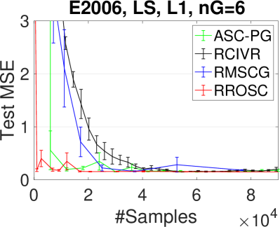
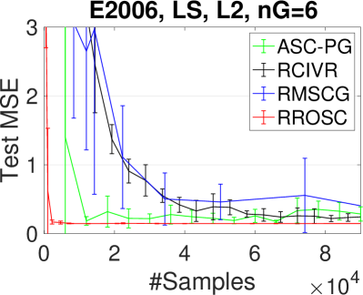
Figure 1: Test MSE error bars: Square loss with $L_{1}$ regularizer (left) and $L_{2}$ regularizer (right). X axis represents the number of samples.

To compare the baseline algorithms, we use mean square error (MSE) as the evaluation metric. We use the original training and testing set for training and testing. To select the hyper-parameters of the four algorithms and the regularizer parameter $\lambda_{reg}$, we randomly select 10% of training data as the validation set. We repeat the experiment for five trials with different random noise and collect the test MSE of each algorithm. We report the error bar results of four algorithms on two problems in Figure 1 to show the average MSE with its standard deviation.

For the regularizer $r(\mathbf{w})$, we employ two commonly used ones, $L_{1}$ regularizer (i.e., $\lambda_{reg}\|\mathbf{w}\|_{1}$) and $L_{2}$ regularizer (i.e., $\frac{\lambda_{reg}}{2}\|\mathbf{w}\|_{2}^{2}$). We choose the value for $\lambda_{reg}$ from the range $\{10^{-5},10^{-4},...,10^{5}\}$. Step size of each algorithm is selected from the range $\{10^{-5},10^{-4},...,10^{5}\}$ on the validation set. The radius $D$ of RROSC is set to $100$.

As clearly shown in Figure 1, our RROSC is more robust than other baselines. First, our RROSC achieves faster convergence in terms of test MSE than others. This supports our theoretical analysis that RROSC has the nearly optimal convergence for stochastic convex compositional problems. Second, the error bars imply that ASC-PG, RCIVR and RMSCG suffer from the large deviation as they converge, while RROSC enjoys a very stable and robust convergence. This verifies the effect of the truncation technique and our high probability convergence under heavy-tailed noise.

7 Conclusion

We have proposed a single-trial stochastic algorithm for convex compositional problems with heavy-tailed noise. We employed the truncation technique in our proposed algorithm to achieve sub-Gaussian confidence bounds by Bernstein inequality. For $\mu$-optimal strongly convex problems, the total sample complexity of our algorithm is $\tilde{O}(1/(\mu\epsilon))$. To the best of our knowledge, this is the first one to establish nearly optimal sub-Gaussian confidence bounds for compositional problems up to a logarithmic factor.

Appendix A Proof of Lemma 1

Proof.

The proof of lemma 1 is two fold. First scenario is the median of means for scalar random variable. Then for multivariate case, we have the robust mean estimation procedure from [11]. Here we present the proof for both.

Case 1: (median of means)
Since $\bar{\mu}_{i}=\frac{1}{m}\sum_{i=1}^{m}X_{i}$ with $X_{i}$ having mean $\mu$ and finite variance $\sigma^{2}$, then $\mathrm{E}[\bar{\mu}_{i}]=\mu$, $\bar{\sigma}^{2}=\frac{\sigma^{2}}{m}$.
By Chebyshev’s inequality, $\mathbb{P}[|\bar{\mu}_{i}-\mu|\leq k_{1}\frac{\sigma}{m}]\geq 1-\frac{1}{k_{1}^{2}}$. Let $k_{1}=2\sqrt{n/k}$. Then we have,

$$\mathbb{P}\Big{[}|\mu_{i}-\mu|\leq\sqrt{\frac{4\sigma^{2}k}{n}}\Big{]}\geq 1-\frac{k}{4n}\geq\frac{3}{4}$$ (12)

Then apply Proposition 5 in [11], we have with $k=8\log(1/\delta)$,

$$\mathbb{P}\Big{[}|\bar{\mu}-\mu|^{2}\leq\frac{32\sigma^{2}\log(1/\delta)}{n}\Big{]}\geq 1-\delta$$ (13)

Case 2: (Robust mean estimator)
Similar to the scalar case, we denote $\bar{\bm{\mu}}_{i}=\frac{1}{m}\sum_{i=1}^{m}X_{i}$ with $X_{i}$. and $\mathrm{E}[\bar{\bm{\mu}}_{i}]=\bm{\mu}$. The variance is defined as the summation of variance of each element. $\bar{\sigma}^{2}=\sum_{i=1}^{d}\frac{\sigma_{i}^{2}}{m}=\frac{\sigma^{2}}{m}$, which is still finite.

By Chebyshev’s inequality for finite dimensional vectors, we have,

$$\mathbb{P}[\|\bar{\bm{\mu}}_{i}-\bm{\mu}\|\leq k_{2}\|\bar{\sigma}\|]>1-\frac{1}{k_{2}^{2}}$$ (14)

$$\Rightarrow \mathbb{P}\Big{[}\|\bar{\bm{\mu}}_{i}-\bm{\mu}\|\leq\sqrt{\frac{3\sigma^{2}k}{n}}\Big{]}\geq 1-\frac{k}{3n}\geq\frac{2}{3}$$ (15)

where we plug in $k_{2}=\sqrt{3n/k}$. If we denote $\varepsilon=\sqrt{\frac{3\sigma^{2}k}{n}}$, and apply Proposition 9 from [11], we will have,

$$\mathbb{P}\big{[}\|\bar{\bm{\mu}}_{i^{*}}-\bm{\mu}\|\leq 3\varepsilon\big{]}\geq 1-e^{-\frac{k}{18}}$$ (16)

Then plug in $k=18\log(1/\delta)$, $\varepsilon=\sqrt{\frac{3\sigma^{2}k}{n}}$ and denote $\bar{\bm{\mu}}=\bar{\bm{\mu}}_{i^{*}}$, we have,

$$\mathbb{P}\Big{[}\|\bar{\bm{\mu}}-\bm{\mu}\|^{2}\leq\frac{486\sigma^{2}\log(1/\delta)}{n}\Big{]}\geq 1-\delta$$ (17)

That concludes the proof of lemma 1. ∎

Appendix B Proofs in Section 4

B.1 Proof of Lemma 2

Before proving Lemma 2, Theorem 1 and Theorem 2, we first provide two useful lemmas, which are proved in the subsequent subsections. The following lemma shows that, under Assumption 1, $f(g(\mathbf{w}))$ has Lipschitz continuous gradients.

Lemma 6.

Suppose Assumption 1 holds. $F(\mathbf{w})$ is $L$-smooth with $L=C_{f}L_{g}+C_{g}^{2}L_{g}$.

The following lemma proves the one-step result for Algorithm 2, which is further used to prove Lemma 2, Theorem 1 and Theorem 2.

Lemma 7.

Suppose Assumption 1 holds. Let $\eta_{t}\leq 1/(2L)$. For Algorithm 2, we have

$$\mathrm{E}[F(\mathbf{w}_{t+1})-F(\mathbf{w})]\leq \frac{1}{2\eta_{t}}\Big{(}\mathrm{E}[\|\mathbf{w}-\mathbf{w}_{t}\|^{2}]-\mathrm{E}[\|\mathbf{w}-\mathbf{w}_{t+1}\|^{2}]\Big{)}$$

$$+\frac{\mu}{4}\mathrm{E}[\|\mathbf{w}-\mathbf{w}_{t}\|^{2}]+2\eta_{t}C_{f}^{2}\frac{\sigma_{1}^{2}}{m_{t}}+2\eta_{t}C_{g}^{2}L_{f}^{2}\frac{\sigma_{0}^{2}}{m_{t}}+\frac{C_{g}^{2}L_{f}^{2}\sigma_{0}^{2}}{\mu m_{t}}$$ (18)

Proof.

Let $\mathbf{w}=\mathbf{w}_{t}^{*}$, where $\mathbf{w}_{t}^{*}$ is the closest point in to $\mathbf{w}_{t}$ in the optimal set. Hence by the $\mu$-optimal strongly convexity of $F(\mathbf{w})$, we have $F(\mathbf{w}_{t})-F(\mathbf{w}_{t}^{*})\geq\frac{\mu}{2}\|\mathbf{w}_{t}-\mathbf{w}_{t}^{*}\|^{2}$.

For (7) of Lemma 7, we let $\eta_{t}=\eta\leq 1/(2L)$, plug in $\mathbf{w}=\mathbf{w}_{t}^{*}$ and summation over over $t=0,...,T-1$ as follows

$$\sum_{t=0}^{T-1}\mathrm{E}[F(\mathbf{w}_{t+1})-F(\mathbf{w}_{t}^{*})]\leq \frac{1}{2\eta}\sum_{t=0}^{T-1}\Big{(}\mathrm{E}[\|\mathbf{w}_{t}^{*}-\mathbf{w}_{t}\|^{2}]-\mathrm{E}[\|\mathbf{w}_{t}^{*}-\mathbf{w}_{t+1}\|^{2}]\Big{)}+\sum_{t=0}^{T-1}\frac{\mu}{4}\mathrm{E}[\|\mathbf{w}_{t}^{*}-\mathbf{w}_{t}\|^{2}]$$

$$+\Big{(}2\eta C_{f}^{2}\sigma_{1}^{2}+2\eta C_{g}^{2}L_{f}^{2}\sigma_{0}^{2}+\frac{C_{g}^{2}L_{f}^{2}\sigma_{0}^{2}}{\mu}\Big{)}\sum_{t=0}^{T-1}\frac{1}{m_{t}}$$

$$\stackrel{{\scriptstyle(a)}}{{\leq}} \frac{1}{2\eta}\sum_{t=0}^{T-1}\Big{(}\mathrm{E}[\|\mathbf{w}_{t}^{*}-\mathbf{w}_{t}\|^{2}]-\mathrm{E}[\|\mathbf{w}_{t+1}^{*}-\mathbf{w}_{t+1}\|^{2}]\Big{)}+\sum_{t=0}^{T-1}\frac{1}{2}\mathrm{E}[F(\mathbf{w}_{t})-F(\mathbf{w}_{t}^{*})]$$

$$+\Big{(}2\eta C_{f}^{2}\sigma_{1}^{2}+2\eta C_{g}^{2}L_{f}^{2}\sigma_{0}^{2}+\frac{C_{g}^{2}L_{f}^{2}\sigma_{0}^{2}}{\mu}\Big{)}\sum_{t=0}^{T-1}\frac{1}{m_{t}}$$

$$= \frac{1}{2\eta}\mathrm{E}[\|\mathbf{w}_{0}^{*}-\mathbf{w}_{0}\|^{2}]-\frac{1}{2\eta}\mathrm{E}[\|\mathbf{w}_{T}^{*}-\mathbf{w}_{T}\|^{2}]+\sum_{t=0}^{T-1}\frac{1}{2}\mathrm{E}[F(\mathbf{w}_{t})-F(\mathbf{w}_{t}^{*})]$$

$$+\Big{(}2\eta C_{f}^{2}\sigma_{1}^{2}+2\eta C_{g}^{2}L_{f}^{2}\sigma_{0}^{2}+\frac{C_{g}^{2}L_{f}^{2}\sigma_{0}^{2}}{\mu}\Big{)}\sum_{t=0}^{T-1}\frac{1}{m_{t}}$$

$$\leq \frac{1}{2\eta}\|\mathbf{w}_{0}^{*}-\mathbf{w}_{0}\|^{2}+\sum_{t=0}^{T-1}\frac{1}{2}\mathrm{E}[F(\mathbf{w}_{t})-F(\mathbf{w}_{t}^{*})]$$

$$+\Big{(}2\eta C_{f}^{2}\sigma_{1}^{2}+2\eta C_{g}^{2}L_{f}^{2}\sigma_{0}^{2}+\frac{C_{g}^{2}L_{f}^{2}\sigma_{0}^{2}}{\mu}\Big{)}\sum_{t=0}^{T-1}\frac{1}{m_{t}}$$

where (a) is due to the definition of $\mathbf{w}_{t}^{*}$ which further implies $\|\mathbf{w}_{t}^{*}-\mathbf{w}_{t+1}\|^{2}\geq\|\mathbf{w}_{t+1}^{*}-\mathbf{w}_{t+1}\|^{2}$.

Re-arranging the above inequality, we have

$$\sum_{t=0}^{T-1}\mathrm{E}[F(\mathbf{w}_{t+1})-F(\mathbf{w}_{t}^{*})]\leq \frac{1}{\eta}\|\mathbf{w}_{0}^{*}-\mathbf{w}_{0}\|^{2}+F(\mathbf{w}_{0})-F(\mathbf{w}_{T})$$

$$+2\Big{(}2\eta C_{f}^{2}\sigma_{1}^{2}+2\eta C_{g}^{2}L_{f}^{2}\sigma_{0}^{2}+\frac{C_{g}^{2}L_{f}^{2}\sigma_{0}^{2}}{\mu}\Big{)}\sum_{t=0}^{T-1}\frac{1}{m_{t}}$$ (20)

Since $\mathbf{w}_{t}^{*}$ is an optimal solution, we have $F(\mathbf{w}_{t}^{*})=F(\mathbf{w}_{t^{\prime}}^{*})$ for any $t$ and $t^{\prime}$. By applying Jensen’s inequality and the convexity of $F$ to LHS of the above (B.1), we have

$$\mathrm{E}[F(\widehat{\mathbf{w}}_{T})-\min_{w}F(\mathbf{w})]\leq \frac{\|\mathbf{w}_{0}^{*}-\mathbf{w}_{0}\|^{2}}{\eta T}+\frac{F(\mathbf{w}_{0})-F(\mathbf{w}_{T})}{T}$$

$$+\frac{2}{T}\Big{(}2\eta C_{f}^{2}\sigma_{1}^{2}+2\eta C_{g}^{2}L_{f}^{2}\sigma_{0}^{2}+\frac{C_{g}^{2}L_{f}^{2}\sigma_{0}^{2}}{\mu}\Big{)}\sum_{t=0}^{T-1}\frac{1}{m_{t}}$$ (21)

where $\widehat{\mathbf{w}}_{T}=\frac{1}{T}\sum_{t=1}^{T}\mathbf{w}_{t}$.
Further by the assumption that $F(\mathbf{w}_{0})-F(\mathbf{w}_{T})\leq\epsilon_{0}$, we obtain Lemma 2.

$$\mathrm{E}[F(\widehat{\mathbf{w}}_{T})-\min_{w}F(\mathbf{w})]\leq \frac{\epsilon_{0}}{T}+\frac{1}{T}\sum_{t=0}^{T-1}\frac{4\eta C_{f}^{2}\sigma_{1}^{2}+4\eta C_{g}^{2}L_{f}^{2}\sigma_{0}^{2}+2C_{g}^{2}L_{f}^{2}\sigma_{0}^{2}/\mu}{m_{t}})+\frac{\|\mathbf{w}_{0}^{*}-\mathbf{w}_{0}\|^{2}}{\eta T}$$

If we let $m_{t}=\frac{t+1}{\mu}$ for $t=0,...,T-1$, then since $\sum_{t=1}^{T}\frac{1}{t}\leq 1+\int_{2}^{T}\frac{1}{t}dt\leq\ln T+1$, we can further have

$$\mathrm{E}[F(\widehat{\mathbf{w}}_{T})-\min_{w}F(\mathbf{w})]\leq \frac{\epsilon_{0}}{T}+\big{(}4\eta C_{f}^{2}\sigma_{1}^{2}+4\eta C_{g}^{2}L_{f}^{2}\sigma_{0}^{2}+2C_{g}^{2}L_{f}^{2}\sigma_{0}^{2}/\mu\big{)}\frac{\ln T+1}{T}+\frac{\|\mathbf{w}_{0}^{*}-\mathbf{w}_{0}\|^{2}}{\eta T}$$

To guarantee $\mathrm{E}[F(\widehat{\mathbf{w}}_{T})-F(\mathbf{w}_{*})]\leq\epsilon$, we require $T=\tilde{O}(1/\epsilon)$ and the total sample complexity is

$$\sum_{t=0}^{T-1}m_{t}=\sum_{t=0}^{T-1}\frac{t+1}{\mu}=\frac{(T+1)T}{2\mu}=\tilde{O}(\frac{1}{\mu\epsilon^{2}}).$$

∎

B.2 Proof for Theorem 1

Proof.

We first consider the convergence of the inner loop. Suppose $F(\mathbf{w}_{0})-F(\mathbf{w}_{*})\leq\epsilon_{0}$, $m_{t}=m=\frac{1}{c\mu\epsilon_{0}}$ where $c=\frac{1}{4(2\mu\eta C_{f}^{2}\sigma_{1}^{2}+2\mu\eta C_{g}^{2}L_{f}^{2}\sigma_{0}^{2}+C_{g}^{2}L_{f}^{2}\sigma_{0}^{2})}$. Starting from (B.1) where we take summation over the one-step result, let $\mathbf{w}=\mathbf{w}_{*}$ and we have

$$\sum_{t=0}^{T-1}\mathrm{E}[F(\mathbf{w}_{t+1})-F(\mathbf{w}_{*})]\leq \frac{1}{2\eta}\|\mathbf{w}_{*}-\mathbf{w}_{0}\|^{2}+\Big{(}2\eta C_{f}^{2}\sigma_{1}^{2}+2\eta C_{g}^{2}L_{f}^{2}\sigma_{0}^{2}+\frac{C_{g}^{2}L_{f}^{2}\sigma_{0}^{2}}{\mu}\Big{)}\sum_{t=0}^{T-1}\frac{1}{m}$$

$$= \frac{1}{2\eta}\|\mathbf{w}_{*}-\mathbf{w}_{0}\|^{2}+\Big{(}2\eta C_{f}^{2}\sigma_{1}^{2}+2\eta C_{g}^{2}L_{f}^{2}\sigma_{0}^{2}+\frac{C_{g}^{2}L_{f}^{2}\sigma_{0}^{2}}{\mu}\Big{)}\sum_{t=0}^{T-1}c\mu\epsilon_{0}$$

$$\leq \frac{F(\mathbf{w}_{0})-F(\mathbf{w}_{*})}{\mu\eta}+\Big{(}2\eta C_{f}^{2}\sigma_{1}^{2}+2\eta C_{g}^{2}L_{f}^{2}\sigma_{0}^{2}+\frac{C_{g}^{2}L_{f}^{2}\sigma_{0}^{2}}{\mu}\Big{)}Tc\mu\epsilon_{0},$$

where the last inequality is due to $\mu$-optimal strong convexity of $F$.

Let $\epsilon_{0}=F(\mathbf{w}_{0})-F(\mathbf{w}_{*})$. Applying Jensen’s inequality to LHS of the above inequality, we have

$$\mathrm{E}[F(\widehat{\mathbf{w}}_{T})-F(\mathbf{w})]\leq \frac{\epsilon_{0}}{\mu\eta T}+\Big{(}2\mu\eta C_{f}^{2}\sigma_{1}^{2}+2\mu\eta C_{g}^{2}L_{f}^{2}\sigma_{0}^{2}+C_{g}^{2}L_{f}^{2}\sigma_{0}^{2}\Big{)}c\epsilon_{0}$$

$$= \frac{\epsilon_{0}}{4}+\frac{\epsilon_{0}}{4}=\frac{\epsilon_{0}}{2},$$

where the last inequality is due to

$$T=\frac{4}{\mu\eta}\text{ and }c=\frac{1}{4(2\mu\eta C_{f}^{2}\sigma_{1}^{2}+2\mu\eta C_{g}^{2}L_{f}^{2}\sigma_{0}^{2}+C_{g}^{2}L_{f}^{2}\sigma_{0}^{2})}.$$

Then we consider the two consecutive loops. Given $F(\mathbf{w}_{k-1})-F(\mathbf{w}_{*})\leq\epsilon_{k-1}$, we have $F(\mathbf{w}_{k})-F(\mathbf{w}_{*})\leq\frac{\epsilon_{k-1}}{2}=\epsilon_{k}$, as long as we set $m_{k}=\frac{1}{c\mu\epsilon_{k-1}}$. To achieve an $\epsilon$-optimal solution, i.e., $\epsilon_{K}\leq\epsilon$, we require $K=\lceil\log(\frac{\epsilon_{0}}{\epsilon})\rceil$, which leads to the total sample complexity

$$m_{tot}=\sum_{k=1}^{K}m_{k}T=\sum_{k=1}^{K}\frac{T}{c\mu}\cdot\frac{1}{\epsilon_{k-1}}=\frac{T}{c\mu}\sum_{k=1}^{K}\frac{2^{k-1}}{\epsilon_{0}}=\frac{T}{c\mu\epsilon_{0}}(2^{K}-1)\leq\frac{4}{c\eta\mu^{2}\epsilon}.$$

∎

B.3 Proof of Lemma 6

Proof.

We prove $f(g(\mathbf{w}))$ has Lipschitz continuous gradients as follows,

$$\|\nabla f(g(\mathbf{w}))\nabla g(\mathbf{w})-\nabla f(g(\mathbf{w}^{\prime}))\nabla g(\mathbf{w}^{\prime})\|$$

$$\stackrel{{\scriptstyle(a)}}{{\leq}} \|\nabla f(g(\mathbf{w}))\nabla g(\mathbf{w})-\nabla f(g(\mathbf{w}))\nabla g(\mathbf{w}^{\prime})\|+\|\nabla f(g(\mathbf{w}))\nabla g(\mathbf{w}^{\prime})-\nabla f(g(\mathbf{w}^{\prime}))\nabla g(\mathbf{w}^{\prime})\|$$

$$= \|\nabla f(g(\mathbf{w}))\|\cdot\|\nabla g(\mathbf{w})-\nabla g(\mathbf{w}^{\prime})\|+\|\nabla g(\mathbf{w}^{\prime})\|\cdot\|\nabla f(g(\mathbf{w}))-\nabla f(g(\mathbf{w}^{\prime}))\|$$

$$\stackrel{{\scriptstyle(b)}}{{\leq}} C_{f}L_{g}\|\mathbf{w}-\mathbf{w}^{\prime}\|+C_{g}L_{g}\|g(\mathbf{w})-g(\mathbf{w}^{\prime})\|$$

$$\stackrel{{\scriptstyle(c)}}{{\leq}} (C_{f}L_{g}+C_{g}^{2}L_{g})\|\mathbf{w}-\mathbf{w}^{\prime}\|,$$

where inequality $(a)$ is due to triangle inequality, inequality $(b)$ is due to $C_{f}$-Lipschitz continuity of $f$, $L_{g}$-smoothness of $g$ and $C_{g}$-Lipschitz continuity of $g$. Inequality $(c)$ is due to $C_{g}$-Lipschitz continuity of $g$. ∎

B.4 Proof of Lemma 7

Proof.

By the optimality of $\mathbf{w}_{t+1}$ of Line 5 of Algorithm 2, we have

$$\langle\nabla f(\mathbf{y}_{t+1})\mathbf{z}_{t+1}+\partial r(\mathbf{w}_{t+1})+\frac{1}{\eta_{t}}(\mathbf{w}_{t+1}-\mathbf{w}_{t}),\mathbf{w}-\mathbf{w}_{t+1}\rangle\geq 0$$

$$\Rightarrow ~{}~{}\langle\nabla f(\mathbf{y}_{t+1})\mathbf{z}_{t+1}+\partial r(\mathbf{w}_{t+1}),\mathbf{w}_{t+1}-\mathbf{w}\rangle\leq\langle\frac{1}{\eta_{t}}(\mathbf{w}_{t+1}-\mathbf{w}_{t}),\mathbf{w}-\mathbf{w}_{t+1}\rangle$$

$$~{}~{}=\frac{1}{\eta_{t}}\langle\mathbf{w}_{t+1}-\mathbf{w}+\mathbf{w}-\mathbf{w}_{t},\mathbf{w}-\mathbf{w}_{t+1}\rangle$$

$$~{}~{}=\frac{1}{\eta_{t}}\Big{(}-\|\mathbf{w}_{t+1}-\mathbf{w}\|+\frac{1}{2}\|\mathbf{w}-\mathbf{w}_{t}\|^{2}+\frac{1}{2}\|\mathbf{w}-\mathbf{w}_{t+1}\|^{2}-\frac{1}{2}\|\mathbf{w}-\mathbf{w}_{t}-\mathbf{w}+\mathbf{w}_{t+1}\|^{2}\Big{)}$$

$$~{}~{}=\frac{1}{2\eta_{t}}\Big{(}\|\mathbf{w}-\mathbf{w}_{t}\|^{2}-\|\mathbf{w}-\mathbf{w}_{t+1}\|^{2}-\|\mathbf{w}_{t}-\mathbf{w}_{t+1}\|^{2}\Big{)}.$$ (24)

For the LHS of the above inequality (B.4), we further have the following lower bound

$$\langle\nabla f(\mathbf{y}_{t+1})\mathbf{z}_{t+1}+\partial r(\mathbf{w}_{t+1}),\mathbf{w}_{t+1}-\mathbf{w}\rangle$$

$$= \langle\nabla f(g(\mathbf{w}_{t}))\nabla g(\mathbf{w}_{t})+\partial r(\mathbf{w}_{t+1}),\mathbf{w}_{t+1}-\mathbf{w}\rangle$$

$$+\langle\nabla f(\mathbf{y}_{t+1})\mathbf{z}_{t+1}-\nabla f(g(\mathbf{w}_{t}))\nabla g(\mathbf{w}_{t}),\mathbf{w}_{t+1}-\mathbf{w}\rangle$$

$$= \langle\nabla f(g(\mathbf{w}_{t}))\nabla g(\mathbf{w}_{t}),\mathbf{w}_{t+1}-\mathbf{w}_{t}+\mathbf{w}_{t}-\mathbf{w}\rangle+\langle\partial r(\mathbf{w}_{t+1}),\mathbf{w}_{t+1}-\mathbf{w}\rangle$$

$$+\langle\nabla f(\mathbf{y}_{t+1})\mathbf{z}_{t+1}-\nabla f(g(\mathbf{w}_{t}))\nabla g(\mathbf{w}_{t}),\mathbf{w}_{t+1}-\mathbf{w}\rangle$$

$$\stackrel{{\scriptstyle(a)}}{{\geq}} \Big{(}f(g(\mathbf{w}_{t+1}))-f(g(\mathbf{w}_{t}))\Big{)}-\frac{L}{2}\|\mathbf{w}_{t+1}-\mathbf{w}_{t}\|^{2}-\Big{(}f(g(\mathbf{w}_{t}))-f(g(\mathbf{w}))\Big{)}$$

$$+r(\mathbf{w}_{t+1})-r(\mathbf{w})+\langle\nabla f(\mathbf{y}_{t+1})\mathbf{z}_{t+1}-\nabla f(g(\mathbf{w}_{t}))\nabla g(\mathbf{w}_{t}),\mathbf{w}_{t+1}-\mathbf{w}\rangle$$

$$= F(\mathbf{w}_{t+1})-F(\mathbf{w})-\frac{L}{2}\|\mathbf{w}_{t+1}-\mathbf{w}_{t}\|^{2}$$

$$+\langle\nabla f(\mathbf{y}_{t+1})\mathbf{z}_{t+1}-\nabla f(g(\mathbf{w}_{t}))\nabla g(\mathbf{w}_{t}),\mathbf{w}_{t+1}-\mathbf{w}\rangle$$ (25)

where inequality $(a)$ is due to convexity of $r$ as well as $L$-smoothness and convexity of $f\circ g$.

Combining the above two inequalities (B.4) and (B.4), we have

$$F(\mathbf{w}_{t+1})-F(\mathbf{w})\leq \frac{1}{2\eta_{t}}\Big{(}\|\mathbf{w}-\mathbf{w}_{t}\|^{2}-\|\mathbf{w}-\mathbf{w}_{t+1}\|^{2}-\|\mathbf{w}_{t}-\mathbf{w}_{t+1}\|^{2}\Big{)}$$

$$+\frac{L}{2}\|\mathbf{w}_{t}-\mathbf{w}_{t+1}\|^{2}$$

$$+\underbrace{\langle\nabla f(g(\mathbf{w}_{t}))\nabla g(\mathbf{w}_{t})-\nabla f(\mathbf{y}_{t+1})\mathbf{z}_{t+1},\mathbf{w}_{t+1}-\mathbf{w}\rangle}_{:=A}.$$ (26)

To upper bound term $A$ in (B.4), we have

$$A= \langle\nabla f(g(\mathbf{w}_{t}))\nabla g(\mathbf{w}_{t})-\nabla f(\mathbf{y}_{t+1})\mathbf{z}_{t+1},\mathbf{w}_{t+1}-\mathbf{w}_{t}+\mathbf{w}_{t}-\mathbf{w}\rangle$$

$$\leq \eta_{t}\|\nabla f(g(\mathbf{w}_{t}))\nabla g(\mathbf{w}_{t})-\nabla f(\mathbf{y}_{t+1})\mathbf{z}_{t+1}\|^{2}+\frac{\|\mathbf{w}_{t}-\mathbf{w}_{t+1}\|^{2}}{4\eta_{t}}$$

$$+\langle\nabla f(g(\mathbf{w}_{t}))\nabla g(\mathbf{w}_{t})-\nabla f(\mathbf{y}_{t+1})\mathbf{z}_{t+1},\mathbf{w}_{t}-\mathbf{w}\rangle,$$ (27)

where the last inequality is due to Young’s inequality.

Plugging (B.4) into (B.4), we finally have

$$F(\mathbf{w}_{t+1})-F(\mathbf{w})\leq \frac{1}{2\eta_{t}}\Big{(}\|\mathbf{w}-\mathbf{w}_{t}\|^{2}-\|\mathbf{w}-\mathbf{w}_{t+1}\|^{2}\Big{)}$$

$$+\Big{(}\frac{L}{2}-\frac{1}{4\eta_{t}}\Big{)}\|\mathbf{w}_{t}-\mathbf{w}_{t+1}\|^{2}$$

$$+\eta_{t}\|\nabla f(g(\mathbf{w}_{t}))\nabla g(\mathbf{w}_{t})-\nabla f(\mathbf{y}_{t+1})\mathbf{z}_{t+1}\|^{2}$$

$$+\langle\nabla f(g(\mathbf{w}_{t}))\nabla g(\mathbf{w}_{t})-\nabla f(\mathbf{y}_{t+1})\mathbf{z}_{t+1},\mathbf{w}_{t}-\mathbf{w}\rangle$$

$$\leq \frac{1}{2\eta_{t}}\Big{(}\|\mathbf{w}-\mathbf{w}_{t}\|^{2}-\|\mathbf{w}-\mathbf{w}_{t+1}\|^{2}\Big{)}$$

$$+\eta_{t}\|\nabla f(g(\mathbf{w}_{t}))\nabla g(\mathbf{w}_{t})-\nabla f(\mathbf{y}_{t+1})\mathbf{z}_{t+1}\|^{2}$$

$$+\langle\nabla f(g(\mathbf{w}_{t}))\nabla g(\mathbf{w}_{t})-\nabla f(\mathbf{y}_{t+1})\mathbf{z}_{t+1},\mathbf{w}_{t}-\mathbf{w}\rangle,$$ (28)

where the last inequality is due to the assumption $\eta_{t}\leq\frac{1}{2L}$.

Recall the following conditions

$$\mathrm{E}[\mathbf{z}_{t+1}]=\nabla g(\mathbf{w}_{t}), \mathrm{E}[\|\mathbf{z}_{t+1}\|^{2}]\leq C_{g}^{2},$$

$$\mathrm{E}[\|\mathbf{z}_{t+1}\|]\leq\sqrt{\mathrm{E}[\|\mathbf{z}_{t+1}\|^{2}]}\leq C_{g}, \mathrm{E}[\nabla f(\cdot)]\leq C_{f}.$$

$$\mathrm{E}[\mathbf{y}_{t+1}-g(\mathbf{w}_{t})\|^{2}]\leq\frac{\sigma_{0}^{2}}{m_{t}}, \mathrm{E}[\|\mathbf{z}_{t+1}-\nabla g(\mathbf{w}_{t})\|^{2}]\leq\frac{\sigma_{1}^{2}}{m_{t}},$$ (29)

By taking expectation conditioned on $\mathbf{w}_{t}$ on both sides of (B.4), we have

$$\mathrm{E}[F(\mathbf{w}_{t+1})-F(\mathbf{w})]$$

$$\leq \frac{1}{2\eta_{t}}\Big{(}\mathrm{E}[\|\mathbf{w}-\mathbf{w}_{t}\|^{2}]-\mathrm{E}[\|\mathbf{w}-\mathbf{w}_{t+1}\|^{2}]\Big{)}$$

$$+\eta_{t}\mathrm{E}[\|\nabla f(g(\mathbf{w}_{t}))\nabla g(\mathbf{w}_{t})-\nabla f(\mathbf{y}_{t+1})\mathbf{z}_{t+1}\|^{2}]$$

$$+\mathrm{E}[\langle\nabla f(g(\mathbf{w}_{t}))\nabla g(\mathbf{w}_{t})-\nabla f(\mathbf{y}_{t+1})\mathbf{z}_{t+1},\mathbf{w}_{t}-\mathbf{w}\rangle]$$

$$\leq \frac{1}{2\eta_{t}}\Big{(}\mathrm{E}[\|\mathbf{w}-\mathbf{w}_{t}\|^{2}]-\mathrm{E}[\|\mathbf{w}-\mathbf{w}_{t+1}\|^{2}]\Big{)}$$

$$+\underbrace{2\eta_{t}\mathrm{E}[\|\nabla f(g(\mathbf{w}_{t}))\nabla g(\mathbf{w}_{t})-\nabla f(g(\mathbf{w}_{t}))\mathbf{z}_{t+1}\|^{2}]}_{:=A}$$

$$+\underbrace{\mathrm{E}[\langle\nabla f(g(\mathbf{w}_{t}))\nabla g(\mathbf{w}_{t})-\nabla f(g(\mathbf{w}_{t}))\mathbf{z}_{t+1},\mathbf{w}_{t}-\mathbf{w}\rangle]}_{:=B}$$

$$+\underbrace{2\eta_{t}\mathrm{E}[\|\nabla f(g(\mathbf{w}_{t}))\mathbf{z}_{t+1}-\nabla f(\mathbf{y}_{t+1})\mathbf{z}_{t+1}\|^{2}]}_{:=C}$$

$$+\underbrace{\mathrm{E}[\langle\nabla f(g(\mathbf{w}_{t}))\mathbf{z}_{t+1}-\nabla f(\mathbf{y}_{t+1})\mathbf{z}_{t+1},\mathbf{w}_{t}-\mathbf{w}\rangle]}_{:=D}.$$ (30)

Then we upper bound the four terms above $A,B,C,D$ by conditions in (B.4) as follows.

$$A\leq 2\eta_{t}\mathrm{E}[\|\nabla f(g(\mathbf{w}_{t}))\|^{2}\cdot\|\nabla g(\mathbf{w}_{t})-\mathbf{z}_{t+1}\|^{2}]\leq 2\eta_{t}C_{f}^{2}\frac{\sigma_{1}^{2}}{m_{t}}.$$ (31)

$$B=\langle\nabla f(g(\mathbf{w}_{t}))\nabla g(\mathbf{w}_{t})-\nabla f(g(\mathbf{w}_{t}))\mathrm{E}[\mathbf{z}_{t+1}],\mathbf{w}_{t}-\mathbf{w}\rangle=0,$$ (32)

where the first equality is due to the fact that $\mathbf{w}_{t}$ is independent on the randomness, and the second inequality is due to $\mathrm{E}[\mathbf{z}_{t+1}]=\nabla g(\mathbf{w}_{t})$ in (B.4).

$$C\leq 2\eta_{t}\mathrm{E}[\|\mathbf{z}_{t+1}\|^{2}\cdot\|\nabla f(g(\mathbf{w}_{t}))-\nabla f(\mathbf{y}_{t+1})\|^{2}]\leq 2\eta_{t}C_{g}^{2}L_{f}^{2}\frac{\sigma_{0}^{2}}{m_{t}}.$$ (33)

$$D\leq \mathrm{E}[\|\mathbf{z}_{t+1}\|\cdot\|\nabla f(g(\mathbf{w}_{t}))-\nabla f(\mathbf{y}_{t+1})\|\cdot\|\mathbf{w}-\mathbf{w}_{t}\|]$$

$$\leq \mathrm{E}[\|\mathbf{z}_{t+1}\|\cdot L_{f}\|g(\mathbf{w}_{t})-\mathbf{y}_{t+1}\|\cdot\|\mathbf{w}-\mathbf{w}_{t}\|]$$

$$\leq \mathrm{E}[\|\mathbf{z}_{t+1}\|]\cdot\mathrm{E}[L_{f}\|g(\mathbf{w}_{t})-\mathbf{y}_{t+1}\|\cdot\|\mathbf{w}-\mathbf{w}_{t}\|]$$

$$\leq \mathrm{E}[C_{g}L_{f}\|g(\mathbf{w}_{t})-\mathbf{y}_{t+1}\|\cdot\|\mathbf{w}-\mathbf{w}_{t}\|]$$

$$\leq \mathrm{E}\Big{[}\frac{C_{g}^{2}L_{f}^{2}}{\mu}\|g(\mathbf{w}_{t})-\mathbf{y}_{t+1}\|^{2}+\frac{\mu\|\mathbf{w}-\mathbf{w}_{t}\|^{2}}{4}\Big{]}$$

$$\leq \frac{C_{g}^{2}L_{f}^{2}\sigma_{0}^{2}}{\mu m_{t}}+\frac{\mu}{4}\mathrm{E}[\|\mathbf{w}-\mathbf{w}_{t}\|^{2}],$$ (34)

where the first inequality is due to Cauchy-Schwarz inequality, the second inequality is due to $L_{f}$-smooth of $f$, the third inequality is due to independence of $\mathcal{S}_{1}$ and $\mathcal{S}_{2}$, the fourth inequality is due to conditions in (B.4), the fifth inequality is due to Young’s inequality, and the last inequality is due to conditions in (B.4).

Plugging (31), (32), (33) and (B.4) into (B.4), we have

$$\mathrm{E}[F(\mathbf{w}_{t+1})-F(\mathbf{w})]$$

$$\leq \frac{1}{2\eta_{t}}\Big{(}\mathrm{E}[\|\mathbf{w}-\mathbf{w}_{t}\|^{2}]-\mathrm{E}[\|\mathbf{w}-\mathbf{w}_{t+1}\|^{2}]\Big{)}+\frac{\mu}{4}\mathrm{E}[\|\mathbf{w}-\mathbf{w}_{t}\|^{2}]$$

$$+2\eta_{t}C_{f}^{2}\frac{\sigma_{1}^{2}}{m_{t}}+2\eta_{t}C_{g}^{2}L_{f}^{2}\frac{\sigma_{0}^{2}}{m_{t}}+\frac{C_{g}^{2}L_{f}^{2}\sigma_{0}^{2}}{\mu m_{t}}$$

$$= \frac{1}{2\eta_{t}}\Big{(}\mathrm{E}[\|\mathbf{w}-\mathbf{w}_{t}\|^{2}]-\mathrm{E}[\|\mathbf{w}-\mathbf{w}_{t+1}\|^{2}]\Big{)}+\frac{\mu}{4}\mathrm{E}[\|\mathbf{w}-\mathbf{w}_{t}\|^{2}]$$

$$+\Big{(}2\eta_{t}C_{f}^{2}\sigma_{1}^{2}+2\eta_{t}C_{g}^{2}L_{f}^{2}\sigma_{0}^{2}+\frac{C_{g}^{2}L_{f}^{2}\sigma_{0}^{2}}{\mu}\Big{)}\frac{1}{m_{t}}$$ (35)

∎

B.5 Proof of Lemma 3

Proof.

(of Lemma 3) Start with the one-step update of (B.4) in proof of Lemma 7. We let $\eta_{t}=\eta\leq 1/(2L)$ and $\mathbf{w}=\mathbf{w}^{*}_{t}$, i.e., the closted optimal solution to $\mathbf{w}_{t}$. Then taking summation over $t=0,...,T-1$, we have

$$\sum_{t=0}^{T-1}F(\mathbf{w}_{t+1})-F(\mathbf{w}_{t}^{*})\leq\frac{1}{2\eta}\sum_{t=0}^{T-1}\Big{(}\|\mathbf{w}_{t}^{*}-\mathbf{w}_{t}\|^{2}-\|\mathbf{w}_{t}^{*}-\mathbf{w}_{t+1}\|^{2}\Big{)}$$

$$+\eta\|\nabla f(g(\mathbf{w}_{t}))\nabla g(\mathbf{w}_{t})-\nabla f(\mathbf{y}_{t+1})\mathbf{z}_{t+1}\|^{2}+\langle\nabla f(g(\mathbf{w}_{t}))\nabla g(\mathbf{w}_{t})-\nabla f(\mathbf{y}_{t+1})\mathbf{z}_{t+1},\mathbf{w}_{t}-\mathbf{w}_{t}^{*}\rangle.$$

For LHS, since the optimal values are equal, i.e., $F(\mathbf{w}_{t}^{*})=F(\mathbf{w}_{t^{\prime}}^{*})$, we apply Jensen’s inequality as follows

$$\frac{1}{T}\sum_{t=0}^{T-1}(F(\mathbf{w}_{t+1})-F(\mathbf{w}^{*}_{t}))\leq\frac{1}{2\eta T}\sum_{t=0}^{T-1}\Big{(}\|\mathbf{w}_{t}^{*}-\mathbf{w}_{t}\|^{2}-\|\mathbf{w}_{t}^{*}-\mathbf{w}_{t+1}\|^{2}\Big{)}$$

$$+\frac{\eta}{T}\sum_{t=0}^{T-1}\|\nabla f(g(\mathbf{w}_{t}))\nabla g(\mathbf{w}_{t})-\nabla f(\mathbf{y}_{t+1})\mathbf{z}_{t+1}\|^{2}+\frac{1}{T}\sum_{t=0}^{T-1}\langle\nabla f(g(\mathbf{w}_{t}))\nabla g(\mathbf{w}_{t})-\nabla f(\mathbf{y}_{t+1})\mathbf{z}_{t+1},\mathbf{w}_{t}-\mathbf{w}_{t}^{*}\rangle$$

$$\leq\frac{1}{2\eta T}\|\mathbf{w}_{0}^{*}-\mathbf{w}_{0}\|^{2}+\frac{\eta}{T}\sum_{t=0}^{T-1}\|\nabla f(g(\mathbf{w}_{t}))\nabla g(\mathbf{w}_{t})-\nabla f(\mathbf{y}_{t+1})\mathbf{z}_{t+1}\|^{2}$$

$$~{}~{}~{}~{}~{}+\frac{1}{T}\sum_{t=0}^{T-1}\langle\nabla f(g(\mathbf{w}_{t}))\nabla g(\mathbf{w}_{t})-\nabla f(\mathbf{y}_{t+1})\mathbf{z}_{t+1},\mathbf{w}_{t}-\mathbf{w}_{t}^{*}\rangle,$$

where the last inequality is due to the definition of $\mathbf{w}_{t}^{*}$: $\|\mathbf{w}_{t+1}^{*}-\mathbf{w}_{t+1}\|\leq\|\mathbf{w}_{t}^{*}-\mathbf{w}_{t+1}\|$. ∎

B.6 Proof of Theorem 2

Proof.

As analyzed, the key is to bound the two terms $A$ and $B$ in (3) of Lemma 3.

$$\frac{1}{T}\sum_{t=0}^{T-1}(F(\mathbf{w}_{t+1})-F(\mathbf{w}^{*}_{t}))\leq\frac{1}{2\eta T}\|\mathbf{w}_{0}^{*}-\mathbf{w}_{0}\|^{2}+\frac{\eta}{T}\underbrace{\sum_{t=0}^{T-1}\|\nabla f(g(\mathbf{w}_{t}))\nabla g(\mathbf{w}_{t})-\nabla f(\mathbf{y}_{t+1})\mathbf{z}_{t+1}\|^{2}}_{A}$$

$$~{}~{}~{}~{}~{}+\frac{1}{T}\underbrace{\sum_{t=0}^{T-1}\langle\nabla f(g(\mathbf{w}_{t}))\nabla g(\mathbf{w}_{t})-\nabla f(\mathbf{y}_{t+1})\mathbf{z}_{t+1},\mathbf{w}_{t}-\mathbf{w}_{t}^{*}\rangle}_{B},$$

which can be further decomposed to

$$A\leq 2\underbrace{\sum_{t=0}^{T-1}\|\nabla g(\mathbf{w}_{t})^{\top}\nabla f(g(\mathbf{w}_{t}))-\nabla g(\mathbf{w}_{t})^{\top}\nabla f(\mathbf{y}_{t+1})\|^{2}}_{A_{1}}$$

$$+2\underbrace{\sum_{t=0}^{T-1}\|\nabla g(\mathbf{w}_{t})^{\top}\nabla f(\mathbf{y}_{t+1})-\mathbf{z}_{t+1}^{\top}\nabla f(\mathbf{y}_{t+1})\|^{2}}_{A_{2}}$$

$$B\leq \underbrace{\sum_{t=0}^{T-1}\langle\nabla g(\mathbf{w}_{t})^{\top}\nabla f(g(\mathbf{w}_{t}))-\mathbf{z}_{t+1}^{\top}\nabla f(g(\mathbf{w}_{t})),\mathbf{w}_{t}-\mathbf{w}_{t}^{*}\rangle}_{B_{1}}$$

$$+\underbrace{\sum_{t=0}^{T-1}\langle\mathbf{z}_{t+1}^{\top}\nabla f(g(\mathbf{w}_{t}))-\mathbf{z}_{t+1}^{\top}\nabla f(\mathbf{y}_{t+1}),\mathbf{w}_{t}-\mathbf{w}_{t}^{*}\rangle}_{B_{2}}$$

Under Assumption 1, these four terms have the following upper bounds:

$$A_{1}\leq \sum_{t=0}^{T-1}\|\mathbf{z}_{t+1}\|^{2}\cdot\|\nabla f(g(\mathbf{w}_{t}))-\nabla f(\mathbf{y}_{t+1})\|^{2}\leq C_{g}^{2}L_{f}^{2}\sum_{t=0}^{T-1}\|g(\mathbf{w}_{t})-\mathbf{y}_{t+1}\|^{2},$$

$$A_{2}\leq \sum_{t=0}^{T-1}\|\nabla f(g(\mathbf{w}_{t}))\|^{2}\cdot\|\nabla g(\mathbf{w}_{t})-\mathbf{z}_{t+1}\|^{2}\leq C_{f}^{2}\sum_{t=0}^{T-1}\|\nabla g(\mathbf{w}_{t})-\mathbf{z}_{t+1}\|^{2},$$

$$B_{1}\leq \sum_{t=0}^{T-1}\|\nabla f(g(\mathbf{w}_{t}))\|\cdot\|\nabla g(\mathbf{w}_{t})-\mathbf{z}_{t+1}\|\cdot\|\mathbf{w}_{t}^{*}-\mathbf{w}_{t}\|$$

$$\leq \sum_{t=0}^{T-1}C_{f}\|\nabla g(\mathbf{w}_{t})-\mathbf{z}_{t+1}\|\cdot\|\mathbf{w}_{t}^{*}-\mathbf{w}_{t}\|\stackrel{{\scriptstyle(a)}}{{\leq}}\frac{2C_{f}^{2}}{\mu}\sum_{t=0}^{T-1}\|\nabla g(\mathbf{w}_{t})-\mathbf{z}_{t+1}\|^{2}+\frac{\mu}{8}\sum_{t=0}^{T-1}\|\mathbf{w}_{t}^{*}-\mathbf{w}_{t}\|^{2}$$

$$B_{2}\leq \sum_{t=0}^{T-1}\|\mathbf{z}_{t+1}\|\cdot\|\nabla f(g(\mathbf{w}_{t}))-\nabla f(\mathbf{y}_{t+1})\|\cdot\|\mathbf{w}_{t}^{*}-\mathbf{w}_{t}\|$$

$$\leq \sum_{t=0}^{T-1}C_{g}L_{f}\|g(\mathbf{w}_{t})-\mathbf{y}_{t+1}\|\cdot\|\mathbf{w}_{t}^{*}-\mathbf{w}_{t}\|$$

$$\stackrel{{\scriptstyle(b)}}{{\leq}} \frac{2C_{g}^{2}L_{f}^{2}}{\mu}\sum_{t=0}^{T-1}\|g(\mathbf{w}_{t})-\mathbf{y}_{t+1}\|^{2}+\frac{\mu}{8}\sum_{t=0}^{T-1}\|\mathbf{w}_{t}^{*}-\mathbf{w}_{t}\|^{2},$$

where inequalities $(a)$ and $(b)$ are due to Young’s inequality.

By Lemma 1, the following inequalities hold with probability at leaset $1-\delta$, respectively.

$$\|g(\mathbf{w}_{t})-\mathbf{y}_{t+1}\|^{2}\leq\frac{486\sigma_{0}^{2}\log(1/\delta)}{m_{t}},~{}~{}~{}~{}\|\nabla g(\mathbf{w}_{t})-\mathbf{z}_{t+1}\|^{2}\leq\frac{486\sigma_{1}^{2}\log(1/\delta)}{m_{t}}.$$

Combining the above upper bounds for $A$ and $B$ together, from (3) we have

$$\frac{1}{T}\sum_{t=0}^{T-1}(F(\mathbf{w}_{t+1})-F(\mathbf{w}_{*}))\leq\frac{\|\mathbf{w}_{0}^{*}-\mathbf{w}_{0}\|^{2}}{2\eta T}+\frac{\mu}{4T}\sum_{t=0}^{T-1}\|\mathbf{w}_{t}^{*}-\mathbf{w}_{t}\|^{2}$$

$$+\frac{1}{T}(2\eta C_{g}^{2}L_{f}^{2}+\frac{2C_{g}^{2}L_{f}^{2}}{\mu})\sum_{t=0}^{T-1}\|g(\mathbf{w}_{t})-\mathbf{y}_{t+1}\|^{2}+\frac{1}{T}(2\eta C_{f}^{2}+\frac{2C_{f}^{2}}{\mu})\sum_{t=0}^{T-1}\|\nabla g(\mathbf{w}_{t})-\mathbf{z}_{t+1}\|^{2}$$

$$\leq\frac{F(\mathbf{w}_{0})-F(\mathbf{w}_{0}^{*})}{\mu\eta T}+\frac{1}{2T}\sum_{t=0}^{T-1}(F(\mathbf{w}_{t})-F(\mathbf{w}_{t}^{*}))$$

$$+2C_{g}^{2}L_{f}^{2}(\eta+\frac{1}{\mu})486\sigma_{0}^{2}\log(1/\delta)\frac{1}{T}\sum_{t=0}^{T-1}\frac{1}{m_{t}}+2C_{f}^{2}(\eta+\frac{1}{\mu})486\sigma_{1}^{2}\log(1/\delta)\frac{1}{T}\sum_{t=0}^{T-1}\frac{1}{m_{t}}.$$

Re-arranging the above inequality, we have

$$\frac{1}{2T}\sum_{t=0}^{T-1}(F(\mathbf{w}_{t+1})-F(\mathbf{w}_{t+1}^{*}))$$

$$\leq\frac{\epsilon_{0}}{\mu\eta T}+\frac{\epsilon_{0}}{2T}+2(\eta+\frac{1}{\mu})(C_{g}^{2}L_{f}^{2}\sigma_{0}^{2}+C_{f}^{2}\sigma_{1}^{2})486\log(1/\delta)\frac{1}{T}\sum_{t=0}^{T-1}\frac{1}{m_{t}}$$

$$=\frac{\epsilon_{0}}{\mu\eta T}+\frac{\epsilon_{0}}{2T}+2(\mu\eta+1)(C_{g}^{2}L_{f}^{2}\sigma_{0}^{2}+C_{f}^{2}\sigma_{1}^{2})486\log(1/\delta)\frac{1}{\mu m}.$$

For LHS, we apply Jensen’s inequality to derive the lower bound $F(\widehat{\mathbf{w}}_{T})-F(\mathbf{w}_{*})$.

To guarantee $F(\widehat{\mathbf{w}}_{T})-F(\mathbf{w}_{*})\leq\frac{\epsilon_{0}}{2}$, we have

$$\frac{\epsilon_{0}}{T}(\frac{2}{\mu\eta}+1)=\frac{\epsilon_{0}}{4}\qquad\Leftarrow\qquad T=4(\frac{2}{\mu\eta}+1)$$

$$4(\mu\eta+1)(C_{g}^{2}L_{f}^{2}\sigma_{0}^{2}+C_{f}^{2}\sigma_{1}^{2})486\log(1/\delta)\frac{1}{\mu m}=\frac{\epsilon_{0}}{4}$$

$$\qquad\qquad\qquad\qquad\qquad\qquad\Leftarrow m=\frac{16}{\mu\epsilon_{0}}(\mu\eta+1)(C_{g}^{2}L_{f}^{2}\sigma_{0}^{2}+C_{f}^{2}\sigma_{1}^{2})486\log(1/\delta).$$

As a result, for Algorithm 3, given $F(\mathbf{w}_{k-1})-F(\mathbf{w}_{*})\leq\epsilon_{k-1}$ at each stage, we require

$$T\geq 4(\frac{2}{\mu\eta}+1),~{}~{}~{}~{}m_{k}\geq\frac{16}{\mu\epsilon_{k-1}}(\mu\eta+1)(C_{g}^{2}L_{f}^{2}\sigma_{0}^{2}+C_{f}^{2}\sigma_{1}^{2})486\log(1/\delta),$$

so that we can guarantee the following inequality holds with probability at least $1-2T\delta$

$$F(\mathbf{w}_{k})-F(\mathbf{w}_{*})\leq\frac{\epsilon_{k-1}}{2}.$$

To reach an $\epsilon$-optimal solution with probability at least $1-2TK\delta$, we also require $K=\lceil\log(\frac{\epsilon_{0}}{\epsilon})\rceil$ and the total sample complexity is

$$m_{tot}=\sum_{k=1}^{K}m_{k}T=\sum_{k=1}^{K}O(\frac{1}{\mu^{2}\epsilon_{k-1}})=O(\frac{1}{\mu^{2}\epsilon}).$$

∎

Appendix C Proofs in Section 5

C.1 Proof of Theorem 3

In this section, we prove Theorem 3. As we mentioned, the key is to bound the two terms $A$ and $B$ in Lemma 3 by making use of the reference truncation technique in (6) and (9).

Proof.

(details of Theorem 3) Start from the one-stage result in Lemma 3. Recall that by the robust estimator, we have $\tilde{\mathbf{y}}_{0}$ and $\tilde{\mathbf{z}}_{0}$ with probability at least $1-2\delta$ such that

$$\|\tilde{\mathbf{y}}_{0}-g(\mathbf{w}_{0})\|\leq\nu\sigma_{0},~{}~{}~{}~{}~{}\|\tilde{\mathbf{z}}_{0}-\nabla g(\mathbf{w}_{0})\|\leq\nu\sigma_{1},$$

which satisfy (6) and (9).

By (3), replacing $\mathbf{y}_{t+1}$ and $\mathbf{z}_{t+1}$ with $\widehat{\mathbf{y}}_{t+1}$ and $\widehat{\mathbf{z}}_{t+1}$, we have

$$F(\widehat{\mathbf{w}}_{T})-F(\mathbf{w}_{*})\leq \frac{\|\mathbf{w}_{0}-\mathbf{w}_{*}\|^{2}}{2\eta T}+\frac{\eta}{T}\sum_{t=0}^{T-1}\|\nabla g(\mathbf{w}_{t})^{\top}\nabla f(g(\mathbf{w}_{t}))-\widehat{\mathbf{z}}_{t+1}^{\top}\nabla f(\widehat{\mathbf{y}}_{t+1})\|^{2}$$

$$+\frac{1}{T}\sum_{t=0}^{T-1}\langle\nabla g(\mathbf{w}_{t})^{\top}\nabla f(g(\mathbf{w}_{t}))-\widehat{\mathbf{z}}_{t+1}^{\top}\nabla f(\widehat{\mathbf{y}}_{t+1}),\mathbf{w}_{t}-\mathbf{w}_{*}\rangle$$

$$\leq \frac{\epsilon_{0}}{\mu\eta T}+\frac{2\eta}{T}\sum_{t=0}^{T-1}\|\nabla g(\mathbf{w}_{t})^{\top}\nabla f(g(\mathbf{w}_{t}))-\nabla g(\mathbf{w}_{t})^{\top}\nabla f(\widehat{\mathbf{y}}_{t+1})\|^{2}$$

$$+\frac{2\eta}{T}\sum_{t=0}^{T-1}\|\nabla g(\mathbf{w}_{t})^{\top}\nabla f(\widehat{\mathbf{y}}_{t+1})-\widehat{\mathbf{z}}_{t+1}^{\top}\nabla f(\widehat{\mathbf{y}}_{t+1})\|^{2}$$

$$+\frac{1}{T}\sum_{t=0}^{T-1}\langle\nabla g(\mathbf{w}_{t})^{\top}\nabla f(g(\mathbf{w}_{t}))-\nabla g(\mathbf{w}_{t})^{\top}\nabla f(\widehat{\mathbf{y}}_{t+1}),\mathbf{w}_{t}-\mathbf{w}_{*}\rangle$$

$$+\frac{1}{T}\sum_{t=0}^{T-1}\langle\nabla g(\mathbf{w}_{t})^{\top}\nabla f(\widehat{\mathbf{y}}_{t+1})-\widehat{\mathbf{z}}_{t+1}^{\top}\nabla f(\widehat{\mathbf{y}}_{t+1}),\mathbf{w}_{t}-\mathbf{w}_{*}\rangle$$

$$\leq \frac{\epsilon_{0}}{\mu\eta T}+\frac{2\eta}{T}\cdot 8C_{g}^{2}L_{f}^{2}(3\log(1/\delta)+2)\max(\sigma_{0}^{2}T/m,C_{g}^{2}D^{2})$$

$$+\frac{2\eta}{T}\cdot 8C_{f}^{2}(3\log(1/\delta)+2)\max(\sigma_{1}^{2}T/m,L_{g}^{2}D^{2})$$

$$+\frac{1}{T}\cdot 8C_{g}L_{f}D(\log(1/\delta)+1)\max(\sigma_{0}\sqrt{T/m},C_{g}D)$$

$$+\frac{1}{T}\cdot 8C_{f}D(\log(1/\delta)+1)\max(\sigma_{1}\sqrt{T/m},L_{g}D),$$ (36)

where the second inequality is due to $\mu$-optimal strong convexity and $F(\mathbf{w}_{0})-F(\mathbf{w}_{*})\leq\epsilon_{0}$, the third inequality holds with probability at least $1-4\delta$ due to the four results in Lemma 4.

Recall $D^{2}=\frac{2\epsilon_{0}}{\mu}$. To guarantee $F(\widehat{\mathbf{w}}_{T})-F(\mathbf{w}_{*})\leq\epsilon_{0}/2$, we need to set the values for $\eta$ and $T$ as follows

$$1) ~{}\frac{\epsilon_{0}}{\mu\eta T}=\frac{\epsilon_{0}}{10}\Leftarrow T=\frac{10}{\mu\eta},$$

$$2) ~{}\frac{2\eta}{T}\cdot 8C_{g}^{2}L_{f}^{2}(3\log(1/\delta)+2)\max(\sigma_{0}^{2}T/m,C_{g}^{2}D^{2})\leq\frac{\epsilon_{0}}{10}\Leftarrow\left\{\begin{array}[]{l}\eta\leq\frac{m\epsilon_{0}}{160\sigma_{0}^{2}C_{g}^{2}L_{f}^{2}(3\log(1/\delta)+2)}\\ \eta\leq\frac{1}{C_{g}\sqrt{32C_{g}^{2}L_{f}^{2}(3\log(1/\delta)+2)}}\end{array}\right.,$$ (39)

$$3) ~{}\frac{2\eta}{T}\cdot 8C_{f}^{2}(3\log(1/\delta)+2)\max(\sigma_{1}^{2}T/m,L_{g}^{2}D^{2})\leq\frac{\epsilon_{0}}{10}\Leftarrow\left\{\begin{array}[]{l}\eta\leq\frac{m\epsilon_{0}}{160\sigma_{1}^{2}C_{f}^{2}(3\log(1/\delta)+2)}\\ \eta\leq\frac{1}{L_{g}\sqrt{32C_{f}^{2}(3\log(1/\delta)+2)}}\end{array}\right.,$$ (42)

$$4) ~{}\frac{1}{T}\cdot 8C_{g}L_{f}D(\log(1/\delta)+1)\max(\sigma_{0}\sqrt{T/m},C_{g}D)\leq\frac{\epsilon_{0}}{10}\Leftarrow\left\{\begin{array}[]{l}\eta\leq\frac{m\epsilon_{0}}{1280\sigma_{0}^{2}C_{g}^{2}L_{f}^{2}(\log(1/\delta)+1)^{2}}\\ \eta\leq\frac{1}{16C_{g}L_{f}(\log(1/\delta)+1)}\end{array}\right.$$ (45)

$$5) ~{}\frac{1}{T}\cdot 8C_{f}D(\log(1/\delta)+1)\max(\sigma_{1}\sqrt{T/m},L_{g}D)\leq\frac{\epsilon_{0}}{10}\Leftarrow\left\{\begin{array}[]{l}\eta\leq\frac{m\epsilon_{0}}{1280\sigma_{1}^{2}C_{f}^{2}(\log(1/\delta)+1)^{2}}\\ \eta\leq\frac{1}{16L_{g}C_{f}(\log(1/\delta)+1)}.\end{array}\right.$$ (48)

We can set $m=O(1)$ as a constant, instead of an increasing number in Theorem 1. Therefore, we can set $\eta=O(\epsilon_{0})$.

Next, we consider the $k$-th and ($k+1$)-th stage of Algorithm 4. Suppose $\|\tilde{\mathbf{y}}_{0}-g(\mathbf{w}_{0})\|\leq\nu\sigma_{0}$ and $\|\tilde{\mathbf{z}}_{0}-\nabla g(\mathbf{w}_{0})\|\leq\nu\sigma_{1}$, which can be guaranteed by robust estimator with high probability $1-2\delta$. Let $F(\mathbf{w}_{k})-F(\mathbf{w}_{*})\leq\epsilon_{k-1}$. Then as shown above, we have probability at least $1-4\delta$ such that $F(\mathbf{w}_{k+1})-F(\mathbf{w}_{*})\leq\epsilon_{k-1}/2$ as long as we properly set $\eta_{k},T_{k}$ and $m_{k}$ for Algorithm 5 according to (C.1).

To guarantee $F(\mathbf{w}_{K})-F(\mathbf{w}_{*})\leq\epsilon$ with probability $1-6K\delta$, we need to set $K=\lceil\log(\epsilon_{0}/\epsilon)\rceil$, which implies the total sample complexity is

$$m_{tot}=\sum_{k=1}^{K}T_{k}=\sum_{k=1}^{K}O(\frac{\log(1/\delta)}{\mu\eta_{k}})=\sum_{k=1}^{K}O(\frac{\log(1/\delta)}{\mu\epsilon_{k}})=O(\frac{\log(1/\delta)}{\mu\epsilon}),$$

where $\eta_{k}=O(1/(\epsilon_{k-1}))$ according to (C.1) and $\epsilon_{k}=\epsilon_{k-1}/2$ by assumption.

Finally, consider the truncation parameter $\lambda_{k}$ as follows

$$\lambda_{k}= O\big{(}\max(\sqrt{T_{k}},D_{k})\big{)}=O\big{(}\max(\sqrt{1/(\mu\eta_{k})},\sqrt{\epsilon_{k-1}/\mu})\big{)}$$

$$= O\big{(}\max(\sqrt{1/(\mu\epsilon_{k-1})},\sqrt{\epsilon_{k-1}/\mu})\big{)}.$$

∎

C.2 Proof of Lemma 4

Before we go through our proof, we first present the following two important lemmas, in which we show six bounds related to $\|\widehat{\mathbf{z}}_{t+1}-\nabla g(\mathbf{w}_{t})\|$ and $\|\widehat{\mathbf{y}}_{t+1}-g(\mathbf{w}_{t})\|$, respectively.

Lemma 8.

Suppose Assumption 1 holds and denote $\hat{\sigma}_{m}^{2}=\sigma_{1}^{2}/m$. We have

$$1) \|\widehat{\mathbf{z}}_{t+1}-\nabla g(\mathbf{w}_{t})\|\leq 2L_{g}\|\mathbf{w}_{t}-\mathbf{w}_{0}\|+2\nu\hat{\sigma}_{m}+\lambda$$

$$2) \|\mathrm{E}[\widehat{\mathbf{z}}_{t+1}-\nabla g(\mathbf{w}_{t})]\|\leq\frac{\hat{\sigma}_{m}^{2}}{\lambda^{2}}(L_{g}\|\mathbf{w}_{t}-\mathbf{w}_{0}\|+\nu\hat{\sigma}_{m})+\frac{\hat{\sigma}_{m}^{2}}{\lambda}$$

$$3) \Big{(}\mathrm{E}[\|\widehat{\mathbf{z}}_{t+1}-\nabla g(\mathbf{w}_{t})\|^{2}]\Big{)}^{1/2}\leq\hat{\sigma}_{m}+(L_{g}\|\mathbf{w}_{t}-\mathbf{w}_{0}\|+\nu\hat{\sigma}_{m})\frac{\hat{\sigma}_{m}}{\lambda}$$

$$4) \|\widehat{\mathbf{z}}_{t+1}-\nabla g(\mathbf{w}_{t})\|^{2}\leq(2L_{g}\|\mathbf{w}_{t}-\mathbf{w}_{0}\|+2\nu\hat{\sigma}_{m}+\lambda)^{2}$$

$$5) \mathrm{E}[\|\widehat{\mathbf{z}}_{t+1}-\nabla g(\mathbf{w}_{t})\|^{2}]\leq(\hat{\sigma}_{m}+(L_{g}\|\mathbf{w}_{t}-\mathbf{w}_{0}\|+\nu\hat{\sigma}_{m})\frac{\hat{\sigma}_{m}}{\lambda})^{2}$$

$$6) \Big{(}\mathrm{E}[\|\widehat{\mathbf{z}}_{t+1}-\nabla g(\mathbf{w}_{t})\|^{4}]\Big{)}^{1/2}\leq(2L_{g}\|\mathbf{w}_{t}-\mathbf{w}_{0}\|+2\nu\hat{\sigma}_{m}+\lambda)\cdot(\hat{\sigma}_{m}+(L_{g}\|\mathbf{w}_{t}-\mathbf{w}_{0}\|+\nu\hat{\sigma}_{m})\frac{\hat{\sigma}_{m}}{\lambda}).$$

Similarly, we can have the following lemma w.r.t. $\|\widehat{\mathbf{y}}_{t+1}-g(\mathbf{w}_{t})\|$.

Lemma 9.

Suppose Assumption 1 holds and denote $\tilde{\sigma}_{m}^{2}=\sigma_{0}^{2}/m$. We have

$$1) \|\widehat{\mathbf{y}}_{t+1}-g(\mathbf{w}_{t})\|\leq 2C_{g}\|\mathbf{w}_{t}-\mathbf{w}_{0}\|+2\nu\tilde{\sigma}_{m}+\lambda$$

$$2) \|\mathrm{E}[\widehat{\mathbf{y}}_{t+1}-g(\mathbf{w}_{t})]\|\leq\frac{\tilde{\sigma}_{m}^{2}}{\lambda^{2}}(C_{g}\|\mathbf{w}_{t}-\mathbf{w}_{0}\|+\nu\tilde{\sigma}_{m})+\frac{\tilde{\sigma}_{m}^{2}}{\lambda}$$

$$3) \Big{(}\mathrm{E}[\|\widehat{\mathbf{y}}_{t+1}-g(\mathbf{w}_{t})\|^{2}]\Big{)}^{1/2}\leq\tilde{\sigma}_{m}+(C_{g}\|\mathbf{w}_{t}-\mathbf{w}_{0}\|+\nu\tilde{\sigma}_{m})\frac{\tilde{\sigma}_{m}}{\lambda}$$

$$4) \|\widehat{\mathbf{y}}_{t+1}-g(\mathbf{w}_{t})\|^{2}\leq(2C_{g}\|\mathbf{w}_{t}-\mathbf{w}_{0}\|+2\nu\tilde{\sigma}_{m}+\lambda)^{2}$$

$$5) \mathrm{E}[\|\widehat{\mathbf{y}}_{t+1}-g(\mathbf{w}_{t})\|^{2}]\leq(\tilde{\sigma}_{m}+(C_{g}\|\mathbf{w}_{t}-\mathbf{w}_{0}\|+\nu\tilde{\sigma}_{m})\frac{\tilde{\sigma}_{m}}{\lambda})^{2}$$

$$6) \Big{(}\mathrm{E}[\|\widehat{\mathbf{y}}_{t+1}-g(\mathbf{w}_{t})\|^{4}]\Big{)}^{1/2}\leq(2C_{g}\|\mathbf{w}_{t}-\mathbf{w}_{0}\|+2\nu\tilde{\sigma}_{m}+\lambda)\cdot(\tilde{\sigma}_{m}+(C_{g}\|\mathbf{w}_{t}-\mathbf{w}_{0}\|+\nu\tilde{\sigma}_{m})\frac{\tilde{\sigma}_{m}}{\lambda}).$$

The following lemma gives Bernstein inequality for Martingale difference sequence.

Lemma 10.

(Lemma 1 in [24], Bernstein inequality for martingales) Suppose $X_{1},...,X_{n}$ is a sequence of random variables such that $0\leq X_{i}\leq 1$. Define the martingale difference sequence $\{Y_{n}=\mathrm{E}[X_{n}|X_{1},...,X_{n-1}]-X_{n}\}$ and note $V_{n}$ the sum of the conditional variances

$$V_{n}=\sum_{i=1}^{n}\mathbb{V}[X_{i}|X_{1},...,X_{i-1}]=\sum_{i=1}^{n}\Big{(}X_{i}-\mathrm{E}[X_{i}|X_{1},...,X_{i-1}]\Big{)}^{2}.$$

Let $S_{n}=\sum_{i=1}^{n}X_{i}$. Then for all $a,b\geq 0$,

$$\mathbb{P}\Big{[}\sum_{i=1}^{n}\mathrm{E}[X_{i}|X_{1},...,X_{i-1}]-S_{n}\geq a,V_{n}\leq b\Big{]}\leq\exp\Big{(}-\frac{a^{2}}{2b+2a/3}\Big{)}.$$

It is can be verified that Bernstein inequality also holds for random variables $L_{1},...,L_{n}$ such that $0\leq L_{i}\leq k$.

$$\mathbb{P}\Big{[}\sum_{i=1}^{n}L_{i}-\sum_{i=1}^{n}\mathrm{E}[L_{i}|L_{1},...,L_{i-1}]\geq a,\sum_{i=1}^{n}\mathbb{V}[L_{i}|L_{1},...,L_{i-1}]\leq b\Big{]}\leq\exp\Big{(}-\frac{a^{2}}{2b+2ak/3}\Big{)},$$

which is the form used in our proofs. We can derive it easily by letting $L_{i}=-k(X_{i}-1)$ in Lemma 10, as suggested in [6].

Proof.

(of Lemma 4)

First of all, we present how we can apply Bernstein inequality to get the confidence bound for the martingale difference sequence. Let $\gamma_{0},...,\gamma_{T-1}$ be a sequence of random variables and we can define the following upper bounds $k$, $r$ and $s$ w.r.t. $\gamma_{t}$:

$$|\gamma_{t}|\leq k,~{}~{}~{}|\mathrm{E}_{t}[\gamma_{t}]|\leq r,~{}~{}~{}\Big{(}\mathrm{E}_{t}[\gamma_{t}^{2}]\Big{)}^{1/2}\leq s,$$

where $\mathrm{E}_{t}$ is the expectation conditioned on $\gamma_{t-1}$. By Bernstein inequality in Lemma 10, for any $\tau>0$, we can find $a>0$ such that

$$\mathbb{P}\Big{[}\sum_{t=0}^{T-1}\gamma_{t}\geq Tr+a(2\tau+1)\Big{]}\leq\mathbb{P}\Big{[}\sum_{t=0}^{T-1}\gamma_{t}\geq\sum_{t=0}^{T-1}\mathrm{E}_{t}[\gamma_{t}]+a(2\tau+1)\Big{]}$$

$$\leq \exp\Big{(}-\frac{(2\tau+1)^{2}a^{2}}{2Ts^{2}+2/3ka(2\tau+1)}\Big{)}\leq\exp\Big{(}-\frac{(2\tau+1)^{2}}{2Ts^{2}/a^{2}+2/3\cdot k(2\tau+1)/a}\Big{)},$$ (49)

where the first inequality is due to $Tr\geq\sum_{t=0}^{T-1}\mathrm{E}_{t}[\gamma_{t}]$. When the following two inequalities hold

$$s\sqrt{T}\leq a,~{}~{}~{}~{}~{}k\leq 3a,$$ (50)

we have

$$\mathbb{P}\Big{[}\sum_{t=0}^{T-1}\gamma_{t}\geq Tr+a(2\tau+1)\Big{]}\leq\exp\Big{(}-\frac{(2\tau+1)^{2}}{2+2(2\tau+1)}\Big{)}\leq\exp(-\tau).$$ (51)

To this end, we need to find $a$ such that $s\sqrt{T}\leq a$ and $k\leq 3a$. Recall that $\nu\leq\sqrt{T}$ and $\lambda=\max(L_{g}D,\sigma_{m}\sqrt{T})+\nu\sigma_{m}$. We show how to prove this lemma in the following.

1) Let $\gamma_{t}=\langle\nabla g(\mathbf{w}_{t})^{\top}\nabla f(\widehat{\mathbf{y}}_{t+1})-\widehat{\mathbf{z}}_{t+1}^{\top}\nabla f(\widehat{\mathbf{y}}_{t+1}),\mathbf{w}_{t}-\mathbf{w}\rangle$ be a random variable conditioned on $\mathbf{w}_{t}$ and $\mathrm{E}_{t}[\cdot]$ denote the expectation conditioned on $\mathbf{w}_{t}$. Recall that $f$ is $C_{f}$ Lipschitz continuous, and $\|\mathbf{w}_{t}-\mathbf{w}\|\leq\|\mathbf{w}_{t}-\mathbf{w}_{0}\|+\|\mathbf{w}_{0}-\mathbf{w}\|\leq 2D$ by Line 6 of Algorithm 5 and the assumption. By the bounds $1),2)$ and $3)$ in Lemma 8, we can define the following notations of $k$, $r$ and $s$ for $\gamma_{t}$.

$$|\gamma_{t}|\leq 2C_{f}D\|\nabla g(\mathbf{w}_{t})-\widehat{\mathbf{z}}_{t+1}\|\leq 2C_{f}D(2L_{g}\|\mathbf{w}_{t}-\mathbf{w}_{0}\|+2\nu\hat{\sigma}_{m}+\lambda)\stackrel{{\scriptstyle\Delta}}{{=}}k,$$

$$|\mathrm{E}[\gamma_{t}]|=\langle\mathrm{E}[(\nabla g(\mathbf{w}_{t})-\widehat{\mathbf{z}}_{t+1})^{\top}\nabla f(\widehat{\mathbf{y}}_{t+1})],\mathbf{w}_{t}-\mathbf{w}\rangle$$

$$\qquad\quad\leq 2C_{f}D\|\mathrm{E}[\nabla g(\mathbf{w}_{t})-\widehat{\mathbf{z}}_{t+1}]\|$$

$$\qquad\quad\leq 2C_{f}D(\frac{\hat{\sigma}_{m}^{2}}{\lambda^{2}}(L_{g}\|\mathbf{w}_{t}-\mathbf{w}_{0}\|+\nu\hat{\sigma}_{m})+\frac{\hat{\sigma}_{m}^{2}}{\lambda})\stackrel{{\scriptstyle\Delta}}{{=}}r,$$

$$\Big{(}\mathrm{E}[\gamma_{t}^{2}]\Big{)}^{1/2}\leq\Big{(}\mathrm{E}[(2C_{f}D)^{2}\|\nabla g(\mathbf{w}_{t})-\widehat{\mathbf{z}}_{t+1}\|^{2}]\Big{)}^{1/2}$$

$$\qquad\qquad\quad=2C_{f}D\Big{(}\mathrm{E}[\|\nabla g(\mathbf{w}_{t})-\widehat{\mathbf{z}}_{t+1}\|^{2}]\Big{)}^{1/2}$$

$$\qquad\qquad\quad\leq 2C_{f}D(\hat{\sigma}_{m}+(L_{g}\|\mathbf{w}_{t}-\mathbf{w}_{0}\|+\nu\hat{\sigma}_{m})\frac{\hat{\sigma}_{m}}{\lambda})\stackrel{{\scriptstyle\Delta}}{{=}}s.$$

Then to make $s\sqrt{T}\leq a$ and $k/3\leq a$ hold, we let $a=4C_{f}D\max(\hat{\sigma}_{m}\sqrt{T},L_{g}D)$:

$$s\sqrt{T}= 2C_{f}D(\hat{\sigma}_{m}+(L_{g}\|\mathbf{w}_{t}-\mathbf{w}_{0}\|+\nu\hat{\sigma}_{m})\frac{\hat{\sigma}_{m}}{\lambda})\sqrt{T}$$

$$\leq 2C_{f}D\cdot 2\hat{\sigma}_{m}\sqrt{T}\leq 4C_{f}D\max(\hat{\sigma}_{m}\sqrt{T},L_{g}D)=a,$$

$$k/3= 2/3C_{f}D(2L_{g}D+2\nu\hat{\sigma}_{m}+\lambda)$$

$$\leq 2/3C_{f}D\cdot 3\lambda=2C_{f}D\lambda$$

$$\leq 2C_{f}D(\max(\hat{\sigma}_{m}\sqrt{T},L_{g}D)+\hat{\sigma}_{m}\sqrt{T})$$

$$\leq 4C_{f}D\max(\hat{\sigma}_{m}\sqrt{T},L_{g}D))=a,$$

which satisfy (50).

We also have the upper bound for $r$ as follows

$$r= 2C_{f}D(\frac{\hat{\sigma}_{m}^{2}}{\lambda^{2}}(L_{g}D+\nu\hat{\sigma}_{m})+\frac{\hat{\sigma}_{m}^{2}}{\lambda})$$

$$\leq 4C_{f}D\frac{\hat{\sigma}_{m}^{2}}{\lambda}=4C_{f}D\frac{\hat{\sigma}_{m}^{2}}{\max(L_{g}D,\hat{\sigma}_{m}\sqrt{T})+\nu\hat{\sigma}_{m}}$$

$$\leq 4C_{f}D\frac{\hat{\sigma}_{m}^{2}}{\sigma_{m}\sqrt{T}}=4C_{f}D\frac{\hat{\sigma}_{m}}{\sqrt{T}},$$

which, with the setting of $a$, implies the LHS of (51):

$$\mathbb{P}\Big{[}\sum_{t=0}^{T-1}\gamma_{t}\geq Tr+4C_{f}D\max(\hat{\sigma}_{m}\sqrt{T},L_{g}D)(2\tau+1)\Big{]}$$

$$\geq \mathbb{P}\Big{[}\sum_{t=0}^{T-1}\gamma_{t}\geq T\cdot 4C_{f}D\frac{\hat{\sigma}_{m}}{\sqrt{T}}+4C_{f}D\max(\hat{\sigma}_{m}\sqrt{T},L_{g}D)(2\tau+1)\Big{]}$$

$$= \mathbb{P}\Big{[}\sum_{t=0}^{T-1}\gamma_{t}\geq 4C_{f}D\hat{\sigma}_{m}\sqrt{T}+4C_{f}D\max(\hat{\sigma}_{m}\sqrt{T},L_{g}D)(2\tau+1)\Big{]}$$

$$\geq \mathbb{P}\Big{[}\sum_{t=0}^{T-1}\gamma_{t}\geq 8C_{f}D\max(\hat{\sigma}_{m}\sqrt{T},L_{g}D)(\tau+1)\Big{]}.$$

Plugging the above lower bound to (51) leads to

$$\mathbb{P}\Big{[}\sum_{t=0}^{T-1}\gamma_{t}\geq 8C_{f}D\max(\hat{\sigma}_{m}\sqrt{T},L_{g}D)(\tau+1)\Big{]}\leq\exp(-\tau).$$

Finally, replacing $\tau=\log(1/\delta)$, we prove the result.

2) This proof is as the one of result 1), where the difference is that we use $C_{g}$-Lipschitz continuity of $g$ in truncation, instead of $L_{g}$-Lipschitz continuity of $\nabla g$. Since the proof is very similar, we skip the proof and state that the following inequality holds with probability at least $1-\delta$:

$$\sum_{t=0}^{T-1}\langle\nabla g(\mathbf{w}_{t})^{\top}\nabla f(g(\mathbf{w}_{t}))-\nabla g(\mathbf{w}_{t})^{\top}\nabla f(\widehat{\mathbf{y}}_{t+1}),\mathbf{w}_{t}-\mathbf{w}\rangle\leq 8C_{g}L_{f}D\max(\tilde{\sigma}_{m}\sqrt{T},C_{g}D).$$

3) Let $\gamma_{t}=\|\nabla g(\mathbf{w}_{t})^{\top}\nabla f(\widehat{\mathbf{y}}_{t+1})-\widehat{\mathbf{z}}_{t+1}^{\top}\nabla f(\widehat{\mathbf{y}}_{t+1})\|^{2}$ be a random variable conditioned on $\mathbf{w}_{t}$. By the bounds $4),5)$ and $6)$ in Lemma 8, we can define the following notations of $k,r$ and $s$ for $\gamma_{t}$:

$$|\gamma_{t}|\leq C_{f}^{2}\|\nabla g(\mathbf{w}_{t})-\widehat{\mathbf{z}}_{t+1}\|^{2}\leq C_{f}^{2}(2L_{g}\|\mathbf{w}_{t}-\mathbf{w}_{0}\|+2\nu\hat{\sigma}_{m}+\lambda)^{2}\stackrel{{\scriptstyle\Delta}}{{=}}k,$$

$$|\mathrm{E}[\gamma_{t}]|=\mathrm{E}[\|\nabla g(\mathbf{w}_{t})^{\top}\nabla f(\widehat{\mathbf{y}}_{t+1})-\widehat{\mathbf{z}}_{t+1}^{\top}\nabla f(\widehat{\mathbf{y}}_{t+1})\|^{2}]\leq C_{f}^{2}\mathrm{E}[\|\nabla g(\mathbf{w}_{t})-\widehat{\mathbf{z}}_{t+1}\|^{2}]$$

$$\qquad\quad\leq C_{f}^{2}(\hat{\sigma}_{m}+(L_{g}\|\mathbf{w}_{t}-\mathbf{w}_{0}\|+\nu\hat{\sigma}_{m})\frac{\hat{\sigma}_{m}}{\lambda})^{2}\stackrel{{\scriptstyle\Delta}}{{=}}r,$$

$$\Big{(}\mathrm{E}[\gamma_{t}^{2}]\Big{)}^{1/2}\leq C_{f}^{2}(2L_{g}\|\mathbf{w}_{t}-\mathbf{w}_{0}\|+2\nu\hat{\sigma}_{m}+\lambda)\cdot(\hat{\sigma}_{m}+(L_{g}\|\mathbf{w}_{t}-\mathbf{w}_{0}\|+\nu\hat{\sigma}_{m})\frac{\hat{\sigma}_{m}}{\lambda})\stackrel{{\scriptstyle\Delta}}{{=}}s.$$

Then to make $s\sqrt{T}\leq a$ and $k/3\leq a$ hold, we let $a=12C_{f}^{2}\max(\hat{\sigma}_{m}^{2}T,L_{g}^{2}D^{2})$:

$$s\sqrt{T}= C_{f}^{2}(2L_{g}\|\mathbf{w}_{t}-\mathbf{w}_{0}\|+2\nu\hat{\sigma}_{m}+\lambda)\cdot(\hat{\sigma}_{m}+(L_{g}\|\mathbf{w}_{t}-\mathbf{w}_{0}\|+\nu\hat{\sigma}_{m})\frac{\hat{\sigma}_{m}}{\lambda})\sqrt{T}$$

$$\leq C_{f}^{2}\cdot 3\lambda\cdot 2\hat{\sigma}_{m}\sqrt{T}=6C_{f}^{2}\hat{\sigma}_{m}\sqrt{T}\cdot(\max(\hat{\sigma}_{m}\sqrt{T},L_{g}D)+\nu\hat{\sigma}_{m})$$

$$\leq 12C_{f}^{2}\max(\hat{\sigma}_{m}^{2}T,L_{g}^{2}D^{2})=a,$$

$$k/3= C_{f}^{2}(3\lambda)^{2}/3=3C_{f}^{2}(\max(\hat{\sigma}_{m}\sqrt{T},L_{g}D)+\nu\hat{\sigma}_{m})^{2}$$

$$\leq 12C_{f}^{2}\max(\hat{\sigma}_{m}^{2}T,L_{g}^{2}D^{2})=a.$$

We also have the upper bound for $r$ as follows

$$r=C_{f}^{2}(\hat{\sigma}_{m}+(L_{g}D+\hat{\sigma}_{m}\sqrt{T})\frac{\hat{\sigma}_{m}}{\lambda})^{2}\leq 4C_{f}^{2}\hat{\sigma}_{m}^{2},$$

where we use $\lambda=\max(\hat{\sigma}_{m}\sqrt{T},D)+\nu\hat{\sigma}_{m}\geq\max(\hat{\sigma}_{m}\sqrt{T},L_{g}D)$ .

Using the above upper bound of $r$ and the setting of $a$, by (51), we have

$$\mathbb{P}\Big{[}\sum_{t=0}^{T-1}\gamma_{t}\geq 8C_{f}^{2}(2+3\tau)\max(\hat{\sigma}_{m}^{2}T,L_{g}^{2}D^{2})\Big{]}$$

$$\leq \mathbb{P}\Big{[}\sum_{t=0}^{T-1}\gamma_{t}\geq 4C_{f}^{2}\hat{\sigma}_{m}^{2}T+12C_{f}^{2}\max(\hat{\sigma}_{m}^{2}T,L_{g}^{2}D^{2})(2\tau+1)\Big{]}$$

$$\leq \mathbb{P}\Big{[}\sum_{t=0}^{T-1}\gamma_{t}\geq Tr+12C_{f}^{2}\max(\hat{\sigma}_{m}^{2}T,L_{g}^{2}D^{2})(2\tau+1)\Big{]}$$

$$\leq \exp(-\tau).$$

Finally, replacing $\tau=\log(1/\delta)$, we prove the result.

4) This proof is as the one of result $3)$, where the difference is that we use $C_{g}$-Lipschitz continuity of $g$ in truncation, instead of $L_{g}$-Lipschitz continuity of $\nabla g$. Since the proof is very similar, we skip the proof and state that the following inequality holds with probability at least $1-\delta$:

$$\sum_{t=0}^{T-1}\|\nabla g(\mathbf{w}_{t})^{\top}\nabla f(g(\mathbf{w}_{t}))-\nabla g(\mathbf{w}_{t})^{\top}\nabla f(\widehat{\mathbf{y}}_{t+1})\|^{2}\leq 8C_{g}^{2}L_{f}^{2}(3\log(1/\delta)+2)\max(\tilde{\sigma}_{m}^{2}T,C_{g}^{2}D^{2}).$$

∎

C.3 Proof of Lemma 8

Proof.

(of Lemma 8) First we define two indicators

$$\chi_{t}={\bf 1}_{\|\mathbf{z}_{t+1}-\tilde{\mathbf{z}}_{0}\|\geq L_{g}\|\mathbf{w}_{t}-\mathbf{w}_{0}\|+\nu\hat{\sigma}_{m}+\lambda},~{}~{}~{}\omega_{t}={\bf 1}_{\|\mathbf{z}_{t+1}-\nabla g(\mathbf{w}_{t})\|\geq\lambda}.$$

It can be verified that $\chi_{t}\leq\omega_{t}$ since $\omega_{t}=1$ is a necessary condition of $\chi_{t}=1$, but not sufficient:

$$\|\mathbf{z}_{t+1}-\tilde{\mathbf{z}}_{0}\|\leq \|\mathbf{z}_{t+1}-\nabla g(\mathbf{w}_{t})\|+\|\nabla g(\mathbf{w}_{t})-\tilde{\mathbf{z}}_{0}\|$$

$$\leq \|\mathbf{z}_{t+1}-\nabla g(\mathbf{w}_{t})\|+\|\nabla g(\mathbf{w}_{t})-\nabla g(\mathbf{w}_{0})\|+\|\nabla g(\mathbf{w}_{0})-\tilde{\mathbf{z}}_{0}\|$$

$$\leq \|\mathbf{z}_{t+1}-\nabla g(\mathbf{w}_{t})\|+L_{g}\|\mathbf{w}_{t}-\mathbf{w}_{0}\|+\nu\hat{\sigma}_{m},$$

where the last inequality is due to $L_{g}$-smoothness of $g$. One one hand, when $\|\mathbf{z}_{t+1}-\nabla g(\mathbf{w}_{t})\|\leq\lambda$, i.e., $\omega_{t}=0$, we must have $\mathbf{z}_{t+1}-\tilde{\mathbf{z}}_{0}\leq\lambda+L_{g}\|\mathbf{w}_{t}-\mathbf{w}_{0}\|+\nu\hat{\sigma}_{m}$, i.e., $\chi_{t}=0$. On the other hand, when $\|\mathbf{z}_{t+1}-\nabla g(\mathbf{w}_{t})\|\geq\lambda$, i.e., $\omega_{t}=1$, it is unknown whether $\mathbf{z}_{t+1}-\tilde{\mathbf{z}}_{0}\geq\lambda+L_{g}\|\mathbf{w}_{t}-\mathbf{w}_{0}\|+\nu\sigma_{m}$, i.e., $\chi_{t}=1$. Therefore, $\omega_{t}\geq\chi_{t}$.

The above inequalities also show

$$\|\nabla g(\mathbf{w}_{t})-\tilde{\mathbf{z}}_{0}\|\leq L_{g}\|\mathbf{w}_{t}-\mathbf{w}_{0}\|+\nu\sigma_{m}.$$

To better show the relation between $\widehat{\mathbf{z}}_{t+1}$ and $\nabla g(\mathbf{w}_{t})$, we can also rewrite the following three equivalent forms:

$$\widehat{\mathbf{z}}_{t+1}-\nabla g(\mathbf{w}_{t})= \chi_{t}(\tilde{\mathbf{z}}_{0}-\nabla g(\mathbf{w}_{t}))+(1-\chi_{t})(\mathbf{z}_{t+1}-\nabla g(\mathbf{w}_{t}))$$ (52)

$$= \chi_{t}(\tilde{\mathbf{z}}_{0}-\mathbf{z}_{t+1})+(\mathbf{z}_{t+1}-\nabla g(\mathbf{w}_{t}))$$ (53)

$$= (1-\chi_{t})(\mathbf{z}_{t+1}-\tilde{\mathbf{z}}_{0})+(\tilde{\mathbf{z}}_{0}-\nabla g(\mathbf{w}_{t})).$$ (54)

$1$) To prove the first inequality, i.e., the absolute bound of $\|\widehat{\mathbf{z}}_{t+1}-\nabla g(\mathbf{w}_{t})\|$, we use (54) and have

$$\|\widehat{\mathbf{z}}_{t+1}-\nabla g(\mathbf{w}_{t})\|= \|(1-\chi_{t})(\mathbf{z}_{t+1}-\tilde{\mathbf{z}}_{0})+(\tilde{\mathbf{z}}_{0}-\nabla g(\mathbf{w}_{t}))\|$$

$$\leq (1-\chi_{t})\|\mathbf{z}_{t+1}-\tilde{\mathbf{z}}_{0}\|+\|\tilde{\mathbf{z}}_{0}-\nabla g(\mathbf{w}_{t})\|$$

$$\leq L_{g}\|\mathbf{w}_{t}-\mathbf{w}_{0}\|+\nu\sigma_{m}+\lambda+L_{g}\|\mathbf{w}_{t}-\mathbf{w}_{0}\|+\nu\sigma_{m}$$

$$= 2(L_{g}\|\mathbf{w}_{t}-\mathbf{w}_{0}\|+\nu\sigma_{m})+\lambda.$$

$2$) To prove the second result w.r.t. $\|\mathrm{E}[\widehat{\mathbf{z}}_{t+1}-\nabla g(\mathbf{w}_{t})]\|$, we first take a closer look to $\mathrm{E}[\widehat{\mathbf{z}}_{t+1}-\nabla g(\mathbf{w}_{t})]$ from the perspective of (53) as follows

$$\mathrm{E}[\widehat{\mathbf{z}}_{t+1}-\nabla g(\mathbf{w}_{t})]= \mathrm{E}[\chi_{t}(\tilde{\mathbf{z}}_{0}-\mathbf{z}_{t+1})+(\mathbf{z}_{t+1}-\nabla g(\mathbf{w}_{t}))]$$

$$= \mathrm{E}[\chi_{t}(\tilde{\mathbf{z}}_{0}-\mathbf{z}_{t+1})]$$

$$= \mathrm{E}[\chi_{t}(\tilde{\mathbf{z}}_{0}-\nabla g(\mathbf{w}_{t})+\nabla g(\mathbf{w}_{t})-\mathbf{z}_{t+1})],$$

where the second equality is due to $\mathrm{E}[\mathbf{z}_{t+1}-\nabla g(\mathbf{w}_{t})]=0$.

Now we consider $\|\mathrm{E}[\widehat{\mathbf{z}}_{t+1}-\nabla g(\mathbf{w}_{t})]\|$ as follows

$$\|\mathrm{E}[\widehat{\mathbf{z}}_{t+1}-\nabla g(\mathbf{w}_{t})]\|= \|\mathrm{E}[\chi_{t}(\tilde{\mathbf{z}}_{0}-\nabla g(\mathbf{w}_{t})+\nabla g(\mathbf{w}_{t})-\mathbf{z}_{t+1})]\|$$

$$\leq \mathrm{E}\|\chi_{t}(\tilde{\mathbf{z}}_{0}-\nabla g(\mathbf{w}_{t})+\nabla g(\mathbf{w}_{t})-\mathbf{z}_{t+1})\|$$

$$\leq \mathrm{E}\|\chi_{t}(\tilde{\mathbf{z}}_{0}-\nabla g(\mathbf{w}_{t}))\|+\mathrm{E}\|\chi_{t}(\nabla g(\mathbf{w}_{t})-\mathbf{z}_{t+1})\|$$

$$= \mathrm{E}[\chi_{t}\|(\tilde{\mathbf{z}}_{0}-\nabla g(\mathbf{w}_{t}))\|]+\mathrm{E}[\chi_{t}\|\nabla g(\mathbf{w}_{t})-\mathbf{z}_{t+1}\|]$$

$$\leq \mathrm{E}[\omega_{t}(L_{g}\|\mathbf{w}_{t}-\mathbf{w}_{0}\|+\nu\sigma_{m})]+\mathrm{E}[\omega_{t}\lambda]$$

$$\leq \frac{\sigma_{m}^{2}}{\lambda^{2}}(L_{g}\|\mathbf{w}_{t}-\mathbf{w}_{0}\|+\nu\sigma_{m})+\frac{\sigma_{m}^{2}}{\lambda},$$

where the first inequality is due to Jensen’s inequality and the convexity of $\|\cdot\|$. The third inequality is due to $\chi_{t}\leq\omega_{t}$. The last inequality is due to Markov inequality for a random variable $X$ and constant $a$:

$$\mathbb{P}[X\geq a]\leq\frac{\mathrm{E}[X]}{a}.$$

Here we specifically have

$$\mathbb{P}[\omega_{t}=1]=\mathbb{P}[\|\mathbf{z}_{t+1}-\nabla g(\mathbf{w}_{t})\|^{2}\geq\lambda^{2}]\leq\frac{\mathrm{E}[\|\mathbf{z}_{t+1}-\nabla g(\mathbf{w}_{t})\|^{2}]}{\lambda^{2}}\leq\frac{\sigma_{m}^{2}}{\lambda^{2}}.$$

$3$) To prove the third result w.r.t. $\Big{(}\mathrm{E}[\|\widehat{\mathbf{z}}_{t+1}-\nabla g(\mathbf{w}_{t})\|^{2}]\Big{)}^{1/2}$, we use (54) and have

$$\Big{(}\mathrm{E}[\|\widehat{\mathbf{z}}_{t+1}-\nabla g(\mathbf{w}_{t})\|^{2}]\Big{)}^{1/2}$$

$$= \Big{(}\mathrm{E}[\chi_{t}\|\tilde{\mathbf{z}}_{0}-\nabla g(\mathbf{w}_{t})\|^{2}]\Big{)}^{1/2}+\Big{(}\mathrm{E}[(1-\chi_{t})\|\mathbf{z}_{t+1}-\nabla g(\mathbf{w}_{t})\|^{2}]\Big{)}^{1/2}$$

$$\leq \Big{(}\mathrm{E}[\chi_{t}\|\tilde{\mathbf{z}}_{0}-\nabla g(\mathbf{w}_{t})\|^{2}]\Big{)}^{1/2}+\Big{(}\mathrm{E}[\|\mathbf{z}_{t+1}-\nabla g(\mathbf{w}_{t})\|^{2}]\Big{)}^{1/2}$$

$$\leq \sigma_{m}+\Big{(}\mathrm{E}[\chi_{t}(L_{g}\|\mathbf{w}_{t}-\mathbf{w}_{0}\|+\nu\sigma_{m})^{2}]\Big{)}^{1/2}$$

$$\leq \sigma_{m}+(L_{g}\|\mathbf{w}_{t}-\mathbf{w}_{0}\|+\nu\sigma_{m})(\mathrm{E}[\omega_{t}])^{1/2}$$

$$\leq \sigma_{m}+(L_{g}\|\mathbf{w}_{t}-\mathbf{w}_{0}\|+\nu\sigma_{m})\frac{\sigma_{m}}{\lambda},$$

where the first inequality is due to $(1-\chi_{t})\leq 1$, the second inequality is due to $\mathrm{E}[\|\mathbf{z}_{t+1}-\nabla g(\mathbf{w}_{t})\|^{2}]\leq\sigma_{m}^{2}$ and $\|\tilde{\mathbf{z}}_{0}-\nabla g(\mathbf{w}_{t})\|\leq L_{g}\|\mathbf{w}_{t}-\mathbf{w}_{0}\|$, the third inequality is due to $\chi_{t}\leq 1$, and the last inequality is due to $\mathrm{E}[\omega_{t}]\leq\frac{\sigma_{m}^{2}}{\lambda^{2}}$.

$4$) For $\|\widehat{\mathbf{z}}_{t+1}-\nabla g(\mathbf{w}_{t})\|^{2}$, we can simply apply the result $1$) for $\|\widehat{\mathbf{z}}_{t+1}-\nabla g(\mathbf{w}_{t})\|$:

$$\|\widehat{\mathbf{z}}_{t+1}-\nabla g(\mathbf{w}_{t})\|^{2}\leq(2L_{g}\|\mathbf{w}_{t}-\mathbf{w}_{0}\|+2\nu\sigma_{m}+\lambda)^{2}.$$

$5$) By applying the third result we have proved, we have

$$\mathrm{E}[\|\widehat{\mathbf{z}}_{t+1}-\nabla g(\mathbf{w}_{t})\|^{2}]\leq\Big{(}\mathrm{E}[\|\widehat{\mathbf{z}}_{t+1}-\nabla g(\mathbf{w}_{t})\|^{2}]\Big{)}^{2/2}=(\sigma_{m}+(L_{g}\|\mathbf{w}_{t}-\mathbf{w}_{0}\|+\nu\sigma_{m})\frac{\sigma_{m}}{\lambda})^{2}.$$

$6$) For the last result, we have

$$\Big{(}\mathrm{E}[\|\widehat{\mathbf{z}}_{t+1}-\nabla g(\mathbf{w}_{t})\|^{4}]\Big{)}^{1/2}$$

$$= \Big{(}\mathrm{E}[\|\widehat{\mathbf{z}}_{t+1}-\nabla g(\mathbf{w}_{t})\|^{2}\cdot\mathrm{E}[\|\widehat{\mathbf{z}}_{t+1}-\nabla g(\mathbf{w}_{t})\|^{2}]\Big{)}^{1/2}$$

$$\leq \Big{(}\mathrm{E}[\|\widehat{\mathbf{z}}_{t+1}-\nabla g(\mathbf{w}_{t})\|^{2}\cdot(2L_{g}\|\mathbf{w}_{t}-\mathbf{w}_{0}\|+2\nu\sigma_{m}+\lambda)\Big{)}^{1/2}$$

$$\leq (2L_{g}\|\mathbf{w}_{t}-\mathbf{w}_{0}\|+2\nu\sigma_{m}+\lambda)\cdot(\sigma_{m}+(L_{g}\|\mathbf{w}_{t}-\mathbf{w}_{0}\|+\nu\sigma_{m})\frac{\sigma_{m}}{\lambda}),$$

where the first and second inequalities are due to results $4$) and $5$), respectively.

We omit the proof of Lemma 9 since it is highly anagolous to the proof of Lemma 8. ∎

Appendix D Proof of Lemma 5

Proof.

Let $F(\mathbf{w})$ denote the objective in (11). Denote a feature-label pair as $\xi=(\mathbf{x},y)$. Since $\mathrm{E}_{\xi\sim\mathbb{P}_{i}}[\mathbf{x}\mathbf{x}^{T}]$ is positive semi-definite, there exist $A_{i}\in\mathbb{R}^{d\times d}$ such that

$$\begin{split}\mathcal{L}_{i}(\mathbf{w})&=\mathrm{E}_{\xi\sim\mathbb{P}_{i}}\ell(\mathbf{w};\xi)=\mathrm{E}_{\xi\sim\mathbb{P}_{i}}[(\mathbf{w}^{T}\mathbf{x}-y)^{2}]\\ &=\mathrm{E}_{\xi\sim\mathbb{P}_{i}}[\mathbf{w}^{T}\mathbf{x}\mathbf{x}^{T}\mathbf{w}-2\mathbf{w}^{T}\mathbf{x}y+y^{2}]\\ &=\mathbf{w}^{T}A_{i}^{T}A_{i}\mathbf{w}-\mathbf{b}_{i}^{T}\mathbf{w}+c_{i}\\ \end{split}$$ (55)

where $\mathbf{b}_{i}=2\mathrm{E}_{\xi\sim\mathbb{P}_{i}}[y\mathbf{x}]$ and $c_{i}=\mathrm{E}_{\xi\sim\mathbb{P}_{i}}[y^{2}]$. Note that the components of $\mathbf{b}_{i}$ and $c_{i}$ are constants that do not depend on $\mathbf{w}$.

And we know there exists $A\in\mathbb{R}^{d\times f}$ is matrix such that $A^{T}A=\sum\limits_{i=1}^{m}p_{i}A_{i}^{T}A_{i}$ since $\sum\limits_{i=1}^{m}p_{i}A_{i}^{T}A_{i}$ is positive semi-positive. Define

$$\begin{split}\phi(\mathbf{w},\mathbf{p})&=\sum\limits_{i=1}^{m}p_{i}\mathcal{L}_{i}(\mathbf{w})-h(\mathbf{p})+r(\mathbf{w})\\ &=\sum\limits_{i=1}^{m}p_{i}\mathbf{w}^{T}A_{i}^{T}A_{i}\mathbf{w}-\sum\limits_{i=1}^{m}\mathbf{b}_{i}^{T}\mathbf{w}+\sum\limits_{i=1}^{m}c_{i}-h(\mathbf{p})+r(\mathbf{w})\\ &=\mathbf{w}^{T}A^{T}A\mathbf{w}-\mathbf{b}^{T}\mathbf{w}+c-h(\mathbf{p})+r(\mathbf{w})\\ &=\|A\mathbf{w}\|_{2}^{2}-\mathbf{b}^{T}\mathbf{w}+c-h(\mathbf{p})+r(\mathbf{w})\end{split}$$ (56)

where $\mathbf{b}=\sum\limits_{i=1}^{m}\mathbf{b}_{i}$, $c=\sum\limits_{i=1}^{m}c_{i}$. Then we have $F(\mathbf{w})=\max\limits_{\mathbf{p}}\phi(\mathbf{w},\mathbf{p})$. For any fixed $\mathbf{p}$, applying Lemma 2 of [8], we know that there is a $\mu>0$ such that

$$\begin{split}\phi(\mathbf{w},\mathbf{p})-\arg\min\limits_{\mathbf{w}^{\prime}}\phi(\mathbf{w}^{\prime},\mathbf{p})\geq\frac{\mu}{2}\|\mathbf{w}-\mathbf{w}^{\prime}\|^{2}\end{split}$$ (57)

Denote $\hat{p}(\mathbf{w})=\arg\max\limits_{\mathbf{p}\in\Delta_{m}}\phi(\mathbf{w},\mathbf{p})$. Let $\mathbf{w}_{*}=\arg\min\limits_{\mathbf{w}}F(\mathbf{w})$, and $\mathbf{p}_{*}=\arg\max\limits_{\mathbf{w}}\phi(\mathbf{w}_{*},\mathbf{p})$, i.e., $(\mathbf{w}_{*},\mathbf{p}_{*})$ is a saddle point of $\phi(\mathbf{w},\mathbf{p})$. Then by (57), we have

$$\frac{\mu}{2}\|\mathbf{w}-\mathbf{w}_{*}\|^{2}\leq\phi(\mathbf{w},\mathbf{p}_{*})-\phi(\mathbf{w}_{*},\mathbf{p}_{*})\leq\phi(\mathbf{w},\hat{p}(\mathbf{w}))-\phi(\mathbf{w}_{*},\mathbf{p}_{*})=F(\mathbf{w})-F(\mathbf{w}_{*})$$ (58)

∎

References

• Audibert and Catoni [2011] Jean-Yves Audibert and Olivier Catoni. Robust linear least squares regression. The Annals of Statistics, 39(5):2766–2794, 2011.
• Bubeck et al. [2013] Sébastien Bubeck, Nicolò Cesa-Bianchi, and Gábor Lugosi. Bandits with heavy tail. IEEE Trans. Inf. Theory, 59(11):7711–7717, 2013.
• Chen et al. [2017] Robert S. Chen, Brendan Lucier, Yaron Singer, and Vasilis Syrgkanis. Robust optimization for non-convex objectives. In Advances in Neural Information Processing Systems 30, pages 4705–4714. Curran Associates, Inc., 2017. URL http://papers.nips.cc/paper/7056-robust-optimization-for-non-convex-objectives.pdf.
• Davis et al. [2019] Damek Davis, Dmitriy Drusvyatskiy, Lin Xiao, and Junyu Zhang. From low probability to high confidence in stochastic convex optimization. CoRR, abs/1907.13307, 2019.
• Ermoliev [1976] Y.M. Ermoliev. Methods of stochastic programming, monographs in optimization and or. Nauka, 1976.
• Freedman [1975] David A Freedman. On tail probabilities for martingales. the Annals of Probability, pages 100–118, 1975.
• Ghadimi and Lan [2013] Saeed Ghadimi and Guanghui Lan. Optimal stochastic approximation algorithms for strongly convex stochastic composite optimization, II: shrinking procedures and optimal algorithms. SIAM J. Optimization, 23(4):2061–2089, 2013.
• Gong and Ye [2014] Pinghua Gong and Jieping Ye. Linear convergence of variance-reduced stochastic gradient without strong convexity. arXiv preprint arXiv:1406.1102, 2014.
• Hazan and Kale [2011] Elad Hazan and Satyen Kale. Beyond the regret minimization barrier: an optimal algorithm for stochastic strongly-convex optimization. In Proceedings of Annual Conference on Learning Theory (COLT), pages 421–436, 2011.
• Hsu and Sabato [2014] Daniel Hsu and Sivan Sabato. Heavy-tailed regression with a generalized median-of-means. In ICML, pages 37–45, 2014.
• Hsu and Sabato [2016] Daniel Hsu and Sivan Sabato. Loss minimization and parameter estimation with heavy tails. Journal of Machine Learning Research, 17(18):1–40, 2016.
• Huo et al. [2018] Zhouyuan Huo, Bin Gu, Ji Liu, and Heng Huang. Accelerated method for stochastic composition optimization with nonsmooth regularization. In Sheila A. McIlraith and Kilian Q. Weinberger, editors, Proceedings of the Thirty-Second AAAI Conference on Artificial Intelligence, (AAAI), pages 3287–3294. AAAI Press, 2018.
• Johnson and Zhang [2013] Rie Johnson and Tong Zhang. Accelerating stochastic gradient descent using predictive variance reduction. In Advances in Neural Information Processing Systems (NIPS), pages 315–323, 2013.
• [14] Lihua Lei and Michael I. Jordan. Less than a single pass: Stochastically controlled stochastic gradient. In Aarti Singh and Xiaojin (Jerry) Zhu, editors, Proceedings of the 20th International Conference on Artificial Intelligence and Statistics (AISTATS), volume 54, pages 148–156.
• Lian et al. [2017] Xiangru Lian, Mengdi Wang, and Ji Liu. Finite-sum composition optimization via variance reduced gradient descent. In Aarti Singh and Xiaojin (Jerry) Zhu, editors, Proceedings of the 20th International Conference on Artificial Intelligence and Statistics (AISTATS), volume 54, pages 1159–1167, 2017.
• Lin et al. [2018] Tianyi Lin, Chenyou Fan, Mengdi Wang, and Michael I. Jordan. Improved oracle complexity for stochastic compositional variance reduced gradient. CoRR, abs/1806.00458, 2018.
• Liu and Wright [2015] Ji Liu and Stephen J. Wright. Asynchronous stochastic coordinate descent: Parallelism and convergence properties. SIAM Journal on Optimization, 25(1):351–376, 2015.
• Liu et al. [2018] Liu Liu, Ji Liu, Cho-Jui Hsieh, and Dacheng Tao. Stochastically controlled stochastic gradient for the convex and non-convex composition problem. CoRR, abs/1809.02505, 2018. URL http://arxiv.org/abs/1809.02505.
• Liu et al. [2019] Liu Liu, Ji Liu, and Dacheng Tao. Dualityfree methods for stochastic composition optimization. IEEE Trans. Neural Networks Learn. Syst., 30(4):1205–1217, 2019.
• Lu et al. [2019] Shiyin Lu, Guanghui Wang, Yao Hu, and Lijun Zhang. Optimal algorithms for lipschitz bandits with heavy-tailed rewards. In Kamalika Chaudhuri and Ruslan Salakhutdinov, editors, Proceedings of the 36th International Conference on Machine Learning, (ICML), volume 97 of Proceedings of Machine Learning Research, pages 4154–4163, 2019.
• Nazin et al. [2019] Alexander V. Nazin, Arkadi S. Nemirovsky, Alexandre B. Tsybakov, and Anatoli B. Juditsky. Algorithms of robust stochastic optimization based on mirror descent method. Automation and Remote Control, 80(9):1607–1627, 2019.
• Nemirovski et al. [2009] Arkadi Nemirovski, Anatoli Juditsky, Guanghui Lan, and Alexander Shapiro. Robust stochastic approximation approach to stochastic programming. SIAM Journal on Optimization, 19:1574–1609, 2009. URL http://dx.doi.org/10.1137/070704277.
• Nemirovsky A.S. and IUdin [c1983.] Arkadii Semenovich. Nemirovsky A.S. and D. B. IUdin. Problem complexity and method efficiency in optimization /. Wiley,, Chichester ;, c1983. "A Wiley-Interscience publication.".
• Peel et al. [2013] Thomas Peel, Sandrine Anthoine, and Liva Ralaivola. Empirical bernstein inequality for martingales: Application to online learning. 2013.
• Qian et al. [2019] Qi Qian, Shenghuo Zhu, Jiasheng Tang, Rong Jin, Baigui Sun, and Hao Li. Robust optimization over multiple domains. In The Thirty-Third AAAI Conference on Artificial Intelligence, AAAI 2019, The Thirty-First Innovative Applications of Artificial Intelligence Conference (AAAI), pages 4739–4746. AAAI Press, 2019.
• Rakhlin et al. [2012] Alexander Rakhlin, Ohad Shamir, and Karthik Sridharan. Making gradient descent optimal for strongly convex stochastic optimization. In Proceedings of the 29th International Conference on Machine Learning (ICML), 2012.
• Wang and Liu [2016] Mengdi Wang and Ji Liu. A stochastic compositional gradient method using markov samples. In Winter Simulation Conference, WSC 2016, Washington, DC, USA, December 11-14, 2016, pages 702–713. IEEE, 2016.
• Wang et al. [2017a] Mengdi Wang, Ethan X. Fang, and Han Liu. Stochastic compositional gradient descent: algorithms for minimizing compositions of expected-value functions. Math. Program., 161(1-2):419–449, 2017a.
• Wang et al. [2017b] Mengdi Wang, Ji Liu, and Ethan X. Fang. Accelerating stochastic composition optimization. J. Mach. Learn. Res., 18:105:1–105:23, 2017b.
• Xu et al. [2016] Yi Xu, Qihang Lin, and Tianbao Yang. Accelerate stochastic subgradient method by leveraging local error bound. CoRR, abs/1607.01027, 2016.
• Xu et al. [2019] Yi Xu, Shenghuo Zhu, Sen Yang, Chi Zhang, Rong Jin, and Tianbao Yang. Learning with non-convex truncated losses by SGD. In Amir Globerson and Ricardo Silva, editors, Proceedings of the Thirty-Fifth Conference on Uncertainty in Artificial Intelligence (UAI), page 244. AUAI Press, 2019.
• Yang et al. [2019] Shuoguang Yang, Mengdi Wang, and Ethan X. Fang. Multilevel stochastic gradient methods for nested composition optimization. SIAM J. Optimization, 29(1):616–659, 2019.
• Yu and Huang [2017] Yue Yu and Longbo Huang. Fast stochastic variance reduced ADMM for stochastic composition optimization. In Carles Sierra, editor, Proceedings of the Twenty-Sixth International Joint Conference on Artificial Intelligence (IJCAI), pages 3364–3370. ijcai.org, 2017.
• Zhang and Xiao [2019a] Junyu Zhang and Lin Xiao. A stochastic composite gradient method with incremental variance reduction. In Hanna M. Wallach, Hugo Larochelle, Alina Beygelzimer, Florence d’Alché-Buc, Emily B. Fox, and Roman Garnett, editors, Advances in Neural Information Processing Systems 32, pages 9075–9085, 2019a.
• Zhang and Xiao [2019b] Junyu Zhang and Lin Xiao. A composite randomized incremental gradient method. In Proceedings of the 36th International Conference on Machine Learning, volume 97, pages 7454–7462, 2019b.
• [36] Lijun Zhang and Zhi-Hua Zhou. \ell_1-regression with heavy-tailed distributions. In Samy Bengio, Hanna M. Wallach, Hugo Larochelle, Kristen Grauman, Nicolò Cesa-Bianchi, and Roman Garnett, editors, Advances in Neural Information Processing Systems 31, pages 1084–1094.