A superconducting circuit realization of combinatorial gauge symmetry

Abstract

We propose a superconducting quantum circuit based on a general symmetry principle – combinatorial gauge symmetry – designed to emulate topologically-ordered quantum liquids and serve as a foundation for the construction of topological qubits. The proposed circuit exhibits rich features: in the classical limit of large capacitances its ground state consists of two superimposed loop structures; one is a crystal of small loops containing disordered $U(1)$ degrees of freedom, and the other is a gas of loops of all sizes associated to $\mathbb{Z}_{2}$ topological order. We show that these classical results carry over to the quantum case, where phase fluctuations arise from the presence of finite capacitances, yielding ${\mathbb{Z}}_{2}$ quantum topological order. A key feature of the exact gauge symmetry is that amplitudes connecting different ${\mathbb{Z}}_{2}$ loop states arise from paths having zero classical energy cost. As a result, these amplitudes are controlled by dimensional confinement rather than tunneling through energy barriers. We argue that this effect may lead to larger energy gaps than previous proposals which are limited by such barriers, potentially making it more likely for a topological phase to be experimentally observable. Finally, we discuss how our superconducting circuit realization of combinatorial gauge symmetry can be implemented in practice.

I Introduction

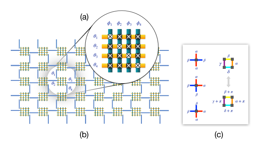
Figure 1: (a) An array of intersecting superconducting wires which form a single “waffle” site in the lattice. Vertical (green) wires are “matter” degrees of freedom with phase $\phi_{n}$ and charge $q_{n}$. Horizontal (yellow) wires are “gauge” degrees of freedom with phase $\theta_{i}$ and charge $Q_{i}$. Wires are coupled by Josephson junctions depicted as black or white crosses depending on the sign of the coupling. This array mirrors the interaction matrix $W$ and implements combinatorial gauge symmetry. (b) The full lattice with links (blue) connecting the gauge degrees of freedom. One site is highlighted to illustrate how sites are connected; links that it shares with neighboring sites are labeled by their gauge phases $\theta_{i}$. The matter wires with phases $\phi_{n}$ are connected only to gauge wires (c) This geometry leads to exact $\mathbb{Z}_{2}$ topological order, as illustrated by the allowed configurations of the gauge phases $\theta$ emanating from each waffle site. We show the limit where the capacitances are large (classical) limit where the gauge phases are good quantum numbers. Gauge phases must be equal pairwise $\alpha$ (red) and $\beta$ (blue) at each site, where both phases are defined modulo $\pi$. In the context of lattice models, such vertices are related to loop models. Additionally, plaquettes may be flipped back and forth by shifting all gauge phases around the plaquette $(\alpha,\beta,\gamma,\delta)$ by $\pi$.

Quantum circuits based on Josephson junctions Devoret et al. (2004) have increasingly leveraged the techniques of large-scale integrated circuit fabrication in recent years, and this technology has become the basis for the largest quantum information processing systems demonstrated to-date King et al. (2018); Arute et al. (2019); Kjaergaard et al. (2020). These circuits can also be engineered to emulate physical quantum systems and basic phenomena, such as the Berezinskii-Kosterlitz-Thouless transition in the XY-model Resnick et al. (1981). The goal of this paper is to describe a superconducting quantum circuit based on a symmetry principle – combinatorial gauge symmetry Chamon et al. (2020) – which can be used to realize topologically ordered states in an engineered quantum system.

The study of topologically ordered states of matter Wen (1990) remains an active area of research in condensed matter physics. This class of states includes, for instance, quantum spin liquids Savary and Balents (2016), which are devoid of magnetic symmetry-breaking order but display topological ground state degeneracies. A number of solvable spin models exist as examples, but these theoretical models include multi-spin interactions not realized in nature. One notable exception of a model with only two-body interactions is the Heisenberg-Kitaev model Kitaev (2006); Jackeli and Khaliullin (2009), but its realization in a material system appears to reside within its non-topological phase.

As opposed to seeking naturally occurring materials, here we follow a similar route to that of Refs. Ioffe et al. (2002); Ioffe and Feigel’man (2002); Douçot et al. (2005, 2003); Gladchenko et al. (2009); Douçot and Ioffe (2012), and focus on engineering topologically ordered systems using superconducting quantum circuits. In the models considered in those works, a gauge symmetry emerges in the limit where the Josephson energy is dominant and the superconducting phase is the good quantum number. Once the correct manifold of states is selected through the Josephson coupling, quantum phase fluctuations induced by the charging energy give rise to a perturbative energy gap that stabilizes the topological phase. The main issue with this emergent symmetry is that it only holds in the perturbative regime where the Josephson energy is much larger than the charging energy.

While the emergent symmetry ensures the existence of the topological phase, its intrinsically perturbative nature fundamentally limits the size of the gaps that can be obtained. One possible way to escape these limits is to design a system for which the gauge symmetry is exact at the microscopic level and therefore non-perturbative, holding for any strength of the coupling constants, including regimes where the charging energy dominates. Such an exact symmetry should therefore expand the range of parameters for which the topological phase may be stable. In this paper we present a proposal for such a system, in the form of a quantum circuit that exhibits exact combinatorial gauge symmetry, including a proposal for how to realize this circuit experimentally.

From a purely theoretical perspective, combinatorial gauge symmetry is interesting in its own right. It can be applied to spins, fermions, or bosons, and all these systems show rich behaviors as a result of the symmetry. We shall present examples of superconducting XY-like systems with coexisting $U(1)$ and ${\mathbb{Z}}_{2}$ loop structures. These two loop structures arise from the form of the designed Josephson couplings: the superconducting phases are locked around the $U(1)$ loops, but only mod $\pi$ (not $2\pi$), as these phases can be shifted by $\pi$ along the closed paths of the ${\mathbb{Z}}_{2}$ loops without changing either the Josephson or the electrostatic energy. We show that the $U(1)$ structure crystallizes into an array of small loops while the ${\mathbb{Z}}_{2}$ structure forms a gas of loops at all scales. These XY-like systems, unlike the usual XY-model, do not show quasi-long-range order of the $U(1)$ degrees of freedom, precisely because of the local loop structures. However, the ${\mathbb{Z}}_{2}$ degrees of freedom realize a topologically ordered state in the same class as in the toric or surface codes, and hence the quantum circuits presented here can be used for building topological qubits.

The paper is organized as follows. In Sec. II we introduce the superconducting circuit that realizes combinatorial gauge symmetry, and we summarize the key elements of this symmetry. In Sec. III we show how topological features naturally arise in the classical limit of large capacitances, in the form of both $U(1)$ and $\mathbb{Z}_{2}$ loop structures. In Sec. IV we discuss how quantum fluctuations endow the loops with dynamics, and how the quantum system is described by an effective toric/surface code Hamiltonian. Finally, in Sec. V we present a detailed discussion of realistic circuit elements needed for an experimental construction.

II Superconducting wire array with combinatorial gauge symmetry

The array of superconducting wires we consider are depicted in Fig. 1. Looking at a given site in Fig. 1(a), each of the four vertical wires is coupled to each of the four horizontal wires by a Josephson junction in a kind of “waffle” geometry. The waffles are placed at the sites of a square lattice, as shown in Fig. 1(b), and are labeled by $s$. The “matter” wires with superconducting phase $\phi_{n}$ are confined to each waffle (or site), and they are indexed by $n$, with $n\in s$ denoting the set of four wires in waffle $s$. The “gauge” wires with phase $\theta_{i}$ are shared between sites, spanning the links or bonds of the square lattice, labeled by $i$, with $i\in s$ denoting the set of four links emanating from site $s$. Each of these phases has a conjugate dimensionless charge variable, satisfying the commutation relations $[\phi_{n},q_{m}]=\mathrm{i}\,\delta_{mn}$ and $[\theta_{i},Q_{j}]=\mathrm{i}\,\delta_{ij}$.

The Hamiltonian for the system is composed of electrostatic (kinetic) and Josephson (potential) terms:

$$H=H_{K}+H_{J}\;.$$ (1)

The kinetic energy is given by:

$$H_{K} =\frac{1}{2}\vec{\mathbf{Q}}^{\rm T}\cdot{\mathbf{C}}^{-1}\cdot\vec{\mathbf{Q}}$$ (2)

where ${\mathbf{C}}^{-1}$ is the system’s inverse capacitance matrix and $\vec{\mathbf{Q}}$ is a vector containing all of the island charges, so that if we define

$$\vec{\mathbf{Q}} \equiv 2e\begin{pmatrix}\vec{Q}\\ \vec{q}\\ \end{pmatrix},\;\vec{\mathbf{\Phi}}\equiv\frac{\Phi_{0}}{2\pi}\begin{pmatrix}\vec{\theta}\\ \vec{\phi}\\ \end{pmatrix}$$ (3)

with $e$ the electron charge and $\Phi_{0}\equiv h/2e$ the superconducting fluxoid quantum, the canonical commutation relations can be re-written as $[\vec{\mathbf{\Phi}},\vec{\mathbf{Q}}]=\hbar\openone$.

The Josephson potential is given by

$$H_{J}=-J\;\sum_{s}\left[\sum_{n,i\in s}W_{ni}\;\cos(\phi_{n}-\theta_{i})\right]$$ (4a)

where we take $$J>0 4\times 4 W \pm 1 W^{\top}W=4\openone$$. The core component is the interaction matrix , which is what enables the combinatorial symmetry and drives the physical connectivity of the circuit. It is required to be a so-called Hadamard matrix whose elements are and it is orthogonal . A convenient choice is

$$W=\begin{pmatrix}-1&+1&+1&+1\\ +1&-1&+1&+1\\ +1&+1&-1&+1\\ +1&+1&+1&-1\end{pmatrix}\;,$$ (4b)

and all other choices are physically equivalent. The coupling matrix is captured literally by the waffle geometry in Fig. 1(a). Hadamard matrices are invariant under a group of monomial transformations, which is the source of the gauge symmetry. Specifically, we have the automorphism

$$L^{-1}\;W\;R=W\;,$$ (5)

where $R$ and $L$ are monomial matrices – generalized permutation matrices with matrix elements $\pm 1$ or 0. Monomial transformations preserve the commutation relations of the underlying operators Chamon et al. (2020), which in this case are the phases and charges on all wires. For example, with our choice of $W$ in Eq. (4b), the following pair satisfies the automorphism (5) on each site $s$:

$$L= \begin{pmatrix}0&+1&0&0\\ +1&0&0&0\\ 0&0&0&-1\\ 0&0&-1&0\end{pmatrix} R= \begin{pmatrix}-1&0&0&0\\ 0&-1&0&0\\ 0&0&+1&0\\ 0&0&0&+1\end{pmatrix}\;.$$ (6)

Here it looks like we are only transforming the interaction, but of course quantum mechanically transforming an operator is equivalent to transforming the state. In this case the $R$ matrix acts on the phases of the gauge wires $\theta_{i}$ on a given site, shifting the phase by $\pi$ whenever there is a $-1$. Similarly, $L$ acts on the phases of the matter wires $\phi_{n}$, shifting them by $\pi$ whenever there is a $-1$, and in such a way as to preserve the required symmetry (5) on each site. The key is that the matter wires are only connected locally on each site, hence their phases may be permuted as well as shifted in general. The gauge wires, on the other hand, bridge two waffles, and therefore the gauge phases can be shifted but not permuted, and hence the matrix $R$ must be diagonal.

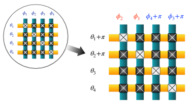
Figure 2: Visual illustration of the action of an $L$ and $R$ pair on the many-body states at each site. The pictured transformation corresponds to the automorphism in Eq. (6) applied to a generic state of the waffle (circle). Note that the signs of the junctions replicate the pattern of $\pm 1$’s in $W$. Wires and couplings are fixed; only the phases are being permuted and/or shifted. Combinatorial gauge symmetry guarantees that the Hamiltonian is invariant under this transformation. The phases of the matter wires can be shifted by $\pi$ and permuted as they only live on that site (permutations indicated by red and blue $\phi$’s). However, states of the gauge wires can be shifted but not permuted as they are shared by neighboring sites. Hence $R$ must be diagonal, but $L$ need only be a monomial matrix. When connected on the lattice, shifting a gauge phase on one site automatically shifts it on its neighboring site, resulting in degenerate states that are loops on the lattice.

The fact that the extra permutation symmetry is local is crucial and gives rise to the topological nature of the waffle circuit. The topological structures that arise in this circuit are illustrated in Fig. 1(c) and discussed in detail in Secs. III and IV below.

Thus far we concentrated on the Josephson couplings in the potential energy term; the capacitance matrix can be quite general for the properties we discuss in the paper, provided the it is symmetric under the permutation of the matter wires within a waffle $s$. Basically, this requirement ensures that $H_{K}$ is invariant under the permutation part of the transformation associated with the $L$ matrices such as those in Eq. (6). We present an experimental setting for such symmetry condition to hold in Sec. V.

Before proceeding with an analysis of the waffle superconducting array, we summarize the mathematical foundation for why it realizes combinatorial gauge symmetry. The general structure will simplify our analysis. And, we will see that the waffle array is a special case, so that the approach can be used to construct other kinds of systems with combinatorial gauge symmetry.

In the most general case, we can write an interaction of the form

$$H_{J}=-J\;\sum_{s}\sum_{n,i\in s}W_{ni}\;\left(\hat{a}^{\dagger}_{n}\;\hat{b}_{i}+\hat{b}^{\dagger}_{i}\;\hat{a}_{n}\right)\;,$$ (7)

where $\hat{a}_{n}$ and $\hat{b}_{i}$ are generic degrees of freedom. In fact we can use any angular momentum, fermionic, or bosonic variables. (Noticeably, when used as a hopping amplitudes for bosons or fermions, the $W$ matrix yields flat bands.) An essential feature is that the $\hat{a}_{n}$ are “matter” fields localized to each site which enables us to use permutation symmetry without distorting the lattice. The $\hat{b}_{i}$ are “gauge” fields which are shared by lattice sites $s$.

According to the automorphism symmetry of $W$ that we have already introduced in Eq. (5) the operators $\hat{a}$ and $\hat{b}$ transform as

$$\hat{a}_{n}\to\sum_{m}\hat{a}_{m}\;(L^{-1})_{mn}\quad\text{and}\quad\hat{b}_{i}\to\sum_{j}R_{ij}\;\hat{b}_{j}\;.$$ (8)

To implement the sign changes in the monomial symmetries, such as those in Eq. (6) we require that there exist unitary transformations $U^{(L)}_{n}$ and $U^{(R)}_{i}$ such that

$$U^{(L)}_{n}\,\hat{a}_{n}^{\phantom{\dagger}}\,U^{(L)\dagger}_{n}=-\hat{a}_{n}\;\;\text{and}\;\;U^{(R)}_{i}\,\hat{b}_{i}^{\phantom{\dagger}}\,U^{(R)\dagger}_{i}=-\hat{b}_{i}\;.$$ (9)

These sign-flip transformations, when combined with permutations of the $n$ and $i$ indices, lead to the monomial transformations written in Eq. (8), which preserve the proper commutation relations of the $\hat{a}$ and $\hat{b}$ operators. We refer to Ref. Chamon et al., 2020 for the special case of how to realize the $\mathbb{Z}_{2}$ gauge theory or toric code using spin-1/2.

To this Hamiltonian $H_{J}$ one can add any kinetic term $H_{K}$ that commutes with the unitary operators $U^{(L)}_{n}$ and $U^{(R)}_{i}$, and that have couplings that are independent of $n$ and $i$, so that permutation invariance holds. In the particular case that the $R$ transformation matrices are restricted to be diagonal, then the couplings need only be independent of $n$, so that the permutation part of the $L$ transformations, see Eq. (6), leaves $H_{K}$ altogether invariant. When these conditions are satisfied, the whole Hamiltonian obeys combinatorial gauge symmetry.

The superconducting wire array is an example of this general framework. In the Hamiltonian with kinetic and potential terms in Eqs. (2) and (4) we identify the matter and gauge fields as the phases of the superconducting wires, as follows:

$$\hat{a}_{n}=e^{\mathrm{i}\,\phi_{n}}\quad \text{and}\quad\hat{b}_{i}=e^{\mathrm{i}\,\theta_{i}}\;,$$

$$U^{(L)}_{n}=e^{\mathrm{i}\pi\,q_{n}}\quad \text{and}\quad U^{(R)}_{i}=e^{\mathrm{i}\pi\,Q_{i}}\;.$$ (10)

$U^{(L)}_{n}$ and $U^{(R)}_{i}$ are generated by the conjugate variables $q_{n}$ and $Q_{i}$, respectively, hence they commute with the kinetic term. The action of $U^{(L)}_{n}$ and $U^{(R)}_{i}$ on $\hat{a}_{n}$ and $\hat{b}_{i}$ can be thought of as shifting $\phi_{n}$ or $\theta_{i}$ by $\pi$. So in addition to the usual global symmetry that shifts all phases equally, we have a local symmetry that shifts an even number of $\theta_{i}$’s and $\phi_{n}$’s by $\pi$ in each star, i.e., each site $s$ with its four links $i\in s$. This transformation can be done consistently on four neighboring stars at the corners of a plaquette $p$; the resulting transformation shifts the phase of the four links on the edges (gauge wires) of the plaquette by $\pi$, along with the corresponding transformations of the matter wires. This transformation is associated with a local ${\mathbb{Z}}_{2}$ symmetry, and we illustrate this operation in Fig. 1(c), on the right.

III Classical loop model

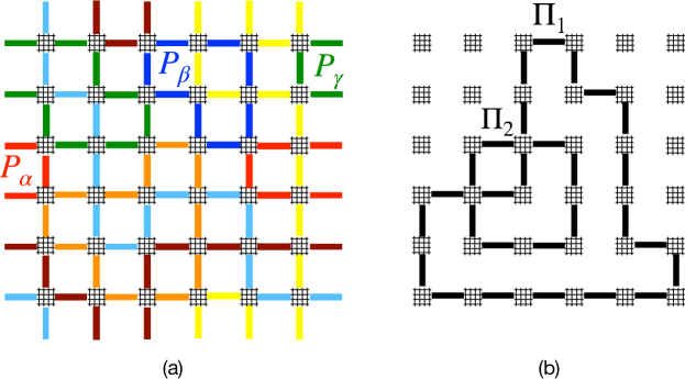
Figure 3: (a) Example of the $U(1)$ loop covering in the superconducting wire array. Values of equal $\theta$ are represented by different colors, and loops wrap around with periodic boundary conditions (e.g., $\theta=\alpha$, $\beta$ and $\gamma$ label three loops $P$ colored red, blue, and green, respectively). Other colored loops fully fill the lattice. Loops can intersect. (b) Example of the second kind of loop $\Pi$, which adds a phase $\pi$ to each of the links visited. Any such loop is a direct result of the local $\mathbb{Z}_{2}$ gauge symmetry and can be superimposed on any loop covering in (a).

We shall show below that a model of loops is realized by the superconducting wire array with combinatorial gauge symmetry. At the minima of $H_{J}$ in Eq. (4), the $\phi_{n}$’s in a waffle $s$ become tethered to the $\theta_{i}$’s:

$$e^{i\phi_{n}}=\frac{\sum_{i\in s}W_{in}\;e^{i\theta_{i}}}{\left|\sum_{i\in s}W_{in}\;e^{i\theta_{i}}\right|},$$ (11)

with the minimum energy given by

$$E_{\rm min}=-J\sum_{s}\sum_{n\in s}\left|\sum_{i\in s}W_{ia}\;e^{i\theta_{i}}\right|\;.$$ (12)

The manifold of minima is such that $\theta_{i}$’s and $\phi_{n}$’s are equal pairwise at each star. On a given site $s$ let us use the short-hand ${\bm{\theta}}=(\theta_{1},\theta_{2},\theta_{3},\theta_{4})$ and similarly for ${\bm{\phi}}$. Then, for instance, the following minima have ground state energy $-8J$ at each site:

$${\bm{\phi}}=(\beta,\alpha,\beta,\alpha)\quad \text{and}\quad{\bm{\theta}}=(\alpha,\beta,\alpha,\beta),$$ (13a)

where $$\alpha \beta 0 2\pi \mathbb{Z}_{2}$$ and are any two phases between and . Moreover, we still have the symmetry. For example, applying the symmetry operation in (6) to (13a) produces another type of minimum,

$${\bm{\phi}}=(\alpha,\beta,\alpha+\pi,\beta+\pi)\quad \text{and}\quad{\bm{\theta}}=(\alpha+\pi,\beta+\pi,\alpha,\beta).$$ (13b)

There are additional minima obtained by symmetry, and their complete set on each site can be visualized as shown in Fig. 1(c). On the entire lattice, these minima must be consistent so the ground states are described by loops as we depict in Fig. 3 with different colors. The lattice Hamiltonian is confined to the valley of minima as long as the phases on the four legs at each site are equal pairwise. Therefore, any fully-packed loop covering – where each site is visited by two loops and each loop has the same phase along its path – will minimize $H_{J}$ of Eq. (4). This class of lattice covering is associated to $U(1)$ or continuous phases, as depicted in Fig. 3(a). In addition, there is another class of loops, associated to the $\mathbb{Z}_{2}$ gauge symmetry. The latter loops do not need to cover all links, but in those links that they do visit, they shift the phases by $\pi$:

$$\theta_{i}\to\theta_{i}+\frac{\pi}{2}(1-\tau^{\rm z}_{i}),\;\;\tau^{\rm z}_{i}=\pm 1,$$ (14)

where $\tau^{\rm z}_{i}=-1$ indicates that a $\pi$ phase shift is added to link $i$, while $\tau^{\rm z}_{i}=+1$ indicates no phase shift to that link. These values can be thought of as the eigenvalues $\pm 1$ of $\tau^{\rm z}_{i}$ operators. Fig. 3(b) depicts the loops of this second kind, or $\mathbb{Z}_{2}$ loops, which follow the sequence of links $i$ with $\tau^{\rm z}_{i}=-1$. We remark that these loops can be generated starting from a reference configuration by the application of generators of the local combinatorial gauge symmetry, plaquette operators [see Eq. (24) for the general case]:

$$G_{p}=\prod_{i\in p}\,e^{\mathrm{i}\pi\,Q_{i}}\,=\,e^{\mathrm{i}\pi\left(\,\sum_{i\in p}Q_{i}\right)}\,=\,\prod_{i\in p}\,\tau^{\rm x}_{i}\;.$$ (15)

where the operators $\tau^{\rm x}_{i}$ flip between the eigenvalues $\pm 1$ of $\tau^{\rm z}_{i}$ operators. Because of the local $\mathbb{Z}_{2}$ symmetry, the $U(1)$ phases of the first kind of loops can be seen as defined mod $\pi$ (rather than $2\pi$), as illustrated by Eqs. (13a) and (13b). Formally, we are working with elements of $U(1)/{\mathbb{Z}}_{2}\cong U(1)$.

In the classical limit of infinite capacitances, we can study the statistical mechanics of the two loop models where the only energy is the $H_{J}$ term of Eq. (4). Even the $T=0$ limit of the model is interesting, in that there is a ground state entropy because of the different ways to cover the lattice with the $U(1)$ and ${\mathbb{Z}}_{2}$ loops. Because these two kinds of loops are independent, the partition function factorizes into the partition functions of two loop models:

$$Z(T=0)=Z^{U(1)}_{\rm loop}\times Z^{{\mathbb{Z}}_{2}}_{\rm loop}\;.$$ (16)

The second component corresponds to the usual $\mathbb{Z}_{2}$ gauge theory. The $U(1)$ component turns out to belong to a class of statistical mechanics models that have been studied in other contexts, such as polymers and lattice spins Chayes et al. (2000); Read and Saleur (2003); Blöte et al. (2012); Nahum et al. (2013). Our case corresponds to the so-called $\text{O}(N)$ loop model, where $N$ is the number of allowed flavors or colors of each loop. Since we have an infinite set of colors our case is the limit $N\to\infty$.

The zero-temperature partition function accounts for all the states that minimize the energy, and encodes the entropic contribution of all allowed loop coverings, hence we can write:

$$Z^{U(1)}_{\rm loop}=\sum_{\rm loop\;coverings}\;\lambda^{n_{\ell}}\;,$$ (17)

where $\lambda$ is the loop fugacity and $n_{\ell}$ is the number of loops in a given loop covering. Since each loop covering is fully packed, the energy associated to loop length is the same for each covering, so we have left an overall ground state energy factor out of the partition function.

We claim that $\lambda\to\infty$ at zero temperature. Intuitively, this is because each closed loop can have an infinite number of colors (continuous phases), so $\lambda$ can be identified with $N$ in this limit. The intuition is made precise by the following counting argument. Take a closed loop visiting $p$ sites and $p$ links. The condition that the phases $\alpha_{p}$ at each site are equal pairwise can be viewed as a series of $p$ Boltzmann weights at some divergent energy scale. However, only $p-1$ constraints are needed because if $\alpha_{1}=\alpha_{2}=\dots=\alpha_{p}$ then automatically $\alpha_{p}=\alpha_{1}$ for a loop. In the limit where the Boltzmann weights become delta functions, the redundant constraint diverges at zero temperature (formally it is an extra delta function “$\delta(0)$”). In the Appendix B we give a simple example to clarify this argument.

Due to the infinite fugacity, the system is driven by entropy to maximize the number of $U(1)$ loops, which is the configuration illustrated in Fig. 4. This ground state is the set of degenerate loop coverings each of which consists of elementary loops of arbitrary phase around every other plaquette. There is no long-range (or quasi-long-range) order of the $U(1)$ loops even at zero temperature. Since the ground state is dominated by small loops, any two links further than one lattice spacing belong to distinct loops and their phases are uncorrelated.

The $\mathbb{Z}_{2}$ loops on the other hand form a loop gas just like in the classical limit of the toric code Castelnovo and Chamon (2007). Because the long loops in the $U(1)$ component are exponentially suppressed, they do not destroy the gapped topological order of the $\mathbb{Z}_{2}$ component.

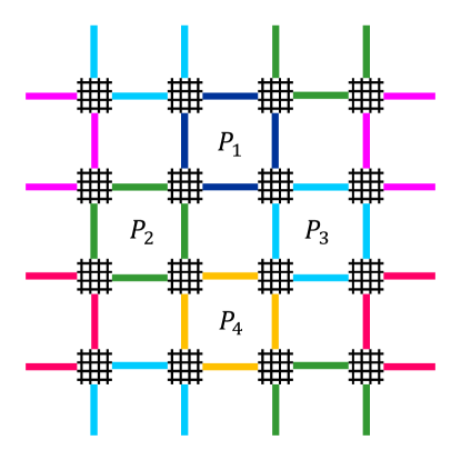
Figure 4: Because the phases defined on the loops vary continuously and independently, the largest entropy configuration maximizes their number; hence it maximizes the number of loops or, equivalently, minimizes the length of each loop. This configuration can be thought of as independently fluctuating phases around loops on alternating plaquettes (depicted by different colors). That this loop crystal has maximum entropy originates from the fact that the “colors” or phases are continuous variables.

IV Quantum loop model:
Emulation of the toric code

The loop models in the previous section originated from the constraints posed on the superconducting phases at the minimum of the Josephson energy for the couplings given by the Hadamard matrix $W$. To endow these loop structures with dynamics, we move away from the classical limit of infinite capacitances. The finite capacitances introduce quantum fluctuations to the superconducting phases $\phi_{n}$ and $\theta_{i}$ via the kinetic energy expressed in terms of the conjugate variables $q_{n}$ and $Q_{i}$. We shall derive an effective quantum Hamiltonian describing the dynamics of the $\mathbb{Z}_{2}$ loops in terms of the $\tau^{\rm z}_{i}$ and $\tau^{\rm x}_{i}$ degrees of freedom discussed in Eqs. (14) and (15).

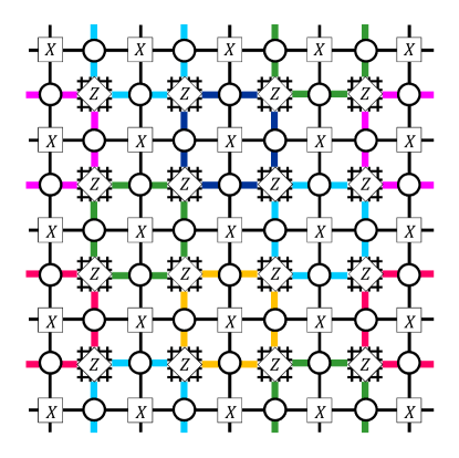
Figure 5: The same lattice as Fig.  4, but with the mapping to the toric code superposed. The qubits in the toric code are indicated by open circles, and are on the links of the lattice. The mapping between the $U(1)$ loops and the toric code star terms is indicated by the label $Z$, and the mapping between the $\mathbb{Z}_{2}$ loops and the toric code plaquette terms is indicated by the label $X$.

The link variables $\tau^{\rm z}_{i}$ play the role of quantum spins, whose two states correspond to the presence or absence of an additional $\pi$ shift on a link. The Josephson coupling penalizes an odd number of $\pi$ shifts on a star, i.e., configurations with $\prod_{i\in s}\tau^{\rm z}_{i}=-1$, which is captured in the effective term

$$H^{\text{eff}}_{\rm star}=-\lambda_{J}\sum_{s}\prod_{i\in s}\tau^{\rm z}_{i}\;,$$ (18)

where $\lambda_{J}=8J$ is the energy separation between the minimum of Eq. (12) (which satisfies $\prod_{i\in s}\tau^{\rm z}_{i}=+1$) and a configuration with an odd number of $\theta_{i}$ variables shifted by $\pi$. $H^{\text{eff}}_{\rm star}$ is the equivalent of the star term in the toric code.

The effective term governing the flip of an elementary (smallest) loop plaquette $p$ is written as

$$H^{\text{eff}}_{\rm plaquette}=-\sum_{p}\lambda_{\rm flip}(p)\prod_{i\in p}\tau^{\rm x}_{i}\;,$$ (19)

which corresponds to the flip operation on a plaquette depicted in Fig. 1(c), on the right. In Eq. (19) we allowed the flipping amplitude $\lambda_{\rm flip}(p)$ to depend on the plaquette $p$, as we detail below, along with how to obtain the scale $\lambda_{\rm flip}$ as function of the capacitances and Josephson coupling.

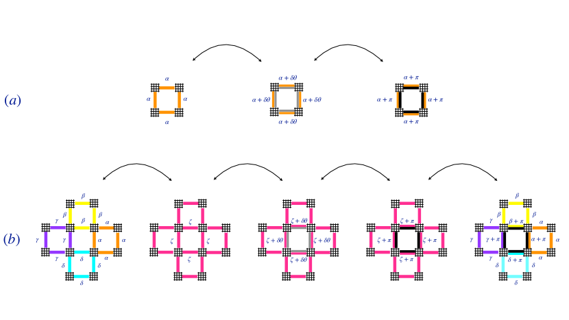
Figure 6: Two types of elementary plaquettes with different plaquette flipping matrix elements. These two types appear as a consequence of the crystal of small loops shown in Fig. 4. In (a) the plaquette contains the elementary $U(1)$ phase variable loop, in which all four phases on the edges are equal to some common angle $\alpha$. In (b) the plaquette is surrounded by four elementary $U(1)$ phase loops, with four different angles $\alpha,\beta,\gamma$ and $\delta$ along the edges. In both cases adding $\pi$ to each leg around the plaquette costs no Josephson energy. The intermediate steps illustrate the path for which one goes from the initial to the final configuration without incurring any Josephson energy penalty.

The effective toric code Hamiltonian consisting of the star term Eq. (18) and plaquette term Eq. (19) is derived by starting from crystal of small loops shown in Fig. 4. For illustration, in Fig. 5 we superpose to Fig. 4 the location of the effective toric spins (at the gauge wires), and the star ($Z$) and plaquette ($X$) operators acting on the $\mathbb{Z}_{2}$ degrees of freedom. To obtain the plaquette flipping amplitudes, we look at the superconducting phase fluctuations around two types of elementary plaquettes: (a) plaquettes which contain an elementary $U(1)$ phase variable loop, in which all four phases on the edges are equal to some common angle $\alpha$; and (b) plaquettes that are surrounded by four elementary $U(1)$ phase loops, with four different angles $\alpha,\beta,\gamma$ and $\delta$ along the edges. [The phases on the matter wires follow those of the gauge wires according to Eq. (13a).] These two cases are illustrated in Fig. 6, on left. Shifting the phases around the four edges of these plaquettes by $\pi$ does not alter the Josephson energy, and these configurations are shown on the right part of Fig. 6. A situation in between the flipped and not flipped cases is shown on the middle part of the figure, for an intermediate shift angle $\delta\theta$. The intermediate configuration for case (a) does not incur an additional Josephson energy cost for any angle $\delta\theta$, because one can vary this angle and always remain in the minimum energy configurations illustrated in Fig. 1(c), on the left. In case (b) there would be a cost if the angles $\alpha,\beta,\gamma$ and $\delta$ are held fixed. However, there is always a path that incurs no Josephson energy cost, illustrated by the intermediate steps in Fig. 6. This path corresponds to changing the four angles $\alpha,\beta,\gamma$ and $\delta$ on the neighboring plaquettes to a common value $\zeta$, then changing the shift angle $\delta\theta$ from 0 to $\pi$, and finally returning from $\zeta$ to the original angles $\alpha,\beta,\gamma$ and $\delta$. Thus, in both cases case (a) or (b) there is no intermediate Josephson energy cost (i.e., no classical energy barrier).

However, the absence of a classical Josephson barrier does not mean that flipping the plaquette is unopposed; quantum fluctuations give rise to an effective barrier. Notice that, in traversing the path in Fig. 6(b), one goes from a 4-dimensional space (defined by the phases $\alpha,\beta,\gamma$ and $\delta$) to another 4-dimensional space where the links are shifted in the middle plaquette by $\pi$. These two 4-dimensional regions are connected by a 2-dimensional constriction (defined by $\zeta$ and $\delta\theta$). This constriction of dimensionality leads to level quantization. The resulting $\delta\theta$-dependent confinement produces an effective barrier along the $\delta\theta$ direction. The height of this barrier can be estimated by treating the transverse motion to $\delta\theta$ as a harmonic oscillator whose potential energy is of order $J$ and whose kinetic energy is controlled by an effective capacitance $C$ which is a function of the physical capacitances of the system. The energy spacing for this harmonic oscillator is the characteristic frequency $\omega=\sqrt{J/C}$. Notice that this energy vanishes in the limit $C\to\infty$, so the effective barrier goes to zero in the classical limit of infinite capacitances, in agreement with our argument that the transitions in Fig. 6 cost no Josephson energy.

A standard WKB approximation using the effective barrier $\sqrt{J/C}$ with kinetic energy at scale $1/C$ leads to the scaling form Gar

$$\lambda_{\rm flip}\sim J\;(JC)^{-k}\;e^{-K\;(JC)^{1/4}}\;.$$ (20)

The precise size of the gap depends on the numerical constants $k,K$ and prefactors in Eq. (20). Nevertheless, notice that the exponent depends on the quartic root of $JC$, a more favorable scaling than the usual square root behavior encountered in other proposals to realize topological phases using superconducting quantum circuits Ioffe et al. (2002); Ioffe and Feigel’man (2002); Douçot et al. (2005, 2003); Gladchenko et al. (2009); Douçot and Ioffe (2012). This qualitative difference is a result of the absence of a classical Josephson energy barrier in our system, which is itself a consequence of the combinatorial gauge symmetry. Moreover, because the combinatorial gauge symmetry is exact for all values of the coupling $J$ and the capacitances, the existence of a topological phase is not limited only to the $JC\gg 1$ regime where the WKB approximation holds, as is the case in previous proposals where the corresponding symmetry is purely emergent Ioffe et al. (2002); Ioffe and Feigel’man (2002); Douçot et al. (2005, 2003); Gladchenko et al. (2009); Douçot and Ioffe (2012). This opens the possibility of achieving much larger gaps by reducing $JC$, as long as the system does not transition to another phase.

Detailed circuit models are needed to identify the effective couplings and the shape of the potentials discussed above. Preliminary calculations Kerman for the full $4\times 4$ lattice of waffles shown in Fig. 4 that include $16\times 4=64$ matter wires, $40$ gauge wires, their self-capacitances, cross-capacitances, and the Josephson junction barrier capacitances $C_{\rm J}$ show that the effective capacitance $C$ above is controlled to leading order by $C_{\rm J}$, and that the frequency $\omega$ above is given to leading order by the Josephson plasma frequency $\sqrt{J/C_{J}}$. Fully quantitative calculation of $\lambda_{\rm flip}$ (or the gap), the limits on its size, and its robustness to disorder and noise are important next steps which we leave for future work.

In summary, here we showed that finite capacitances lead to a quantum $\mathbb{Z}_{2}$ loop model

$$H^{\text{eff}}=H^{\text{eff}}_{\rm star}+H^{\text{eff}}_{\rm plaquette}\;,$$ (21)

where $H^{\text{eff}}_{\rm star}$ and $H^{\text{eff}}_{\rm plaquette}$ are given by Eqs. (18) and (19), respectively. In other words, we generated the toric or surface code Hamiltonian in the superconducting array. Therefore the superconducting circuit we introduced can serve as a platform for building topological qubits.

We close this section by commenting that there is a possibility that the topological phase may even survive the limit of large charging energies if voltage biases are tuned so two nearly degenerate charge states are favored in both matter and gauge wires. In this limit we reach an interesting spin-1/2 system with two-body interactions and an exact ${\mathbb{Z}}_{2}$ gauge symmetry. We describe this “WXY” model in Appendix C, and discuss open questions associated with it.

V Superconducting circuit realization

We now discuss how the system shown in Figs. 1(a) and (b) can be realized in practice. In addition to implementing the Josephson potential described by Eqs. (4) and  (4b), our circuit must also maintain the required symmetry of the Hamiltonian in the presence of unavoidable experimental disorder in circuit parameters. This disorder results both from static imperfections in physical parameters such as Josephson junction sizes and capacitances (both discussed below), as well as the presence of nonstationary ($\sim$1/f) microscopic noise in flux and charge that occur ubiquitously in superconducting circuits Geerligs et al. (1990); Kuzmin et al. (1989); Zimmerli et al. (1992); Ithier et al. (2005); Yoshihara et al. (2006); Bylander et al. (2011); Yan et al. (2016). Of course, in the presence of such disorder, no real-world circuit can ever exhibit perfect combinatorial symmetry, and the success of our proposals will rely on keeping the residual disorder that cannot be removed by design, calibration, or adjustment small enough so as to be only a weak perturbation to the observable physical phenomena of interest. Also, we stress that the topological phases that we seek to realize are protected by an energy gap, so the residual disorder only needs to be suppressed but not necessarily eliminated entirely; as long as the residual imperfections can be treated perturbatively, they do not destroy the topological state.

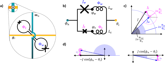
Figure 7: Realistic circuit for a single site of the lattice in Fig. 1. Panel (a) shows how each Josephson junction in Fig. 1(a) is replaced by an asymmetric DC SQUID (b), whose two arms are individually flux-biased with fluxes $\Phi_{w}$ and $\Phi_{t}$. Panel (c) illustrates how the effective total Josephson potential for the SQUID can be viewed schematically with a phasor diagram, in which the two Josephson energies $J_{\rm w}$ and $J_{\rm t}$ can be viewed as adding vectorially. Panel (d) then shows how tuning the two fluxes can be used to realize the correct $\pm 1$ elements of the $W$ matrix in Eq. 4b. Shaded arrows in these panels indicate how adjustments to these fluxes can also be used to null out spurious, small variations in the Josephson energies due to fabrication imperfections.

V.1 Josephson potential

The first and most obvious task in formulating an experimentally-realistic circuit is to produce the Josephson potential of Eq. (4) with the $W$ given in Eq. (4b). To do this we can exploit the fact that a $c$-number offset of $\pi$ of the gauge invariant phase difference across a Josephson junction effectively reverses the sign of its Josephson energy: $J\cos{(\phi+\pi)}=-J\cos{\phi}$. Such offsets can be easily realized in superconducting circuits with closed loops using external magnetic flux, due to the Meissner effect. Although the “waffle” geometry naturally presents us with such closed loops in the form of the plaquettes, each interrupted by four junctions, it is readily seen that applying flux through these loops will not allow us to achieve to desired outcome: for each plaquette containing nine loops we must independently control sixteen $c$-number phase offsets. (Note that in the presence of flux noise we cannot hope to take advantage of any clever geometric scheme exploiting the fact that many of the offsets are the same; we must require that each $c$-number offset can be independently controlled and can be used to null out spurious quasi-static noise.) In addition, relationship between fluxes threading the plaquettes and parameters in the circuit Hamiltonian will be complex and nonlinear, not only because wire segments are shared by numbers of loops, but also higher-order effects such as spatially non-uniform Meissner screening of the external fields and imperfect symmetry of individual wire segments’ self-inductances.

A viable circuit scheme for achieving the required Hamiltonian control is shown in Fig. 7. First, instead of threading flux through the plaquette loops, one can use ancillary loops that replace the single Josephson junction connecting the two wires at each crossing, as depicted in Fig. 7(a). Each of these loops contains two independently-biased (via fluxes $\Phi_{\rm w}$ and $\Phi_{\rm t}$) “arms,” each of which contains one Josephson junction, with the two junctions differing in size by a large factor (chosen, as we discuss below, based on the width of the $J$ distribution for nominally identical junctions due to fabrication process variation). The resulting connection between every pair of crossing wires is then a highly-asymmetric DC SQUID (direct-current superconducting quantum interference device), as shown in Fig. 7(b), which can be used to control the tunneling of Cooper pairs between the two wires. We note that, in this circuit, it will still be experimentally necessary to control the fluxes through the plaquettes; however, this control will consist purely of “magnetic shielding,” in that we want all plaquette fluxes to be zero. Fig. 7(c) illustrates how the two control parameters $\Phi_{\rm w}$ and $\Phi_{\rm t}$ are used, graphically representing the two Cooper pair tunneling amplitudes as phasors, whose magnitudes are given by the two Josephson energies, and whose angles in the complex plane are given by the two external fluxes $\Phi_{\rm w}$ and $\Phi_{\rm t}$. In this simplified picture, the total Josephson potential can be approximated (neglecting the finite geometric inductance of the two arms) as:

$$H_{J,ni}=-J\cos{\left(\phi_{n}-\theta_{i}+2\pi\frac{\Phi_{\rm tot}}{\Phi_{0}}\right)}\;,$$ (22)

with the definitions:

$$J \equiv|J_{\rm w}e^{2\pi i\Phi_{\rm w}/\Phi_{0}}+J_{\rm t}e^{2\pi i\Phi_{\rm t}/\Phi_{0}}|$$

$$2\pi\frac{\Phi_{\rm tot}}{\Phi_{0}} \equiv{\rm Arg}[J_{\rm w}e^{2\pi i\Phi_{\rm w}/\Phi_{0}}+J_{\rm t}e^{2\pi i\Phi_{\rm t}/\Phi_{0}}]\;,$$ (23)

where the effective Josephson energy is given by the norm of the vector sum of the two phasors, and the $c$-number offset to its gauge-invariant phase difference by the argument of that vector sum (see appendix E for details).

The solid arrows in panel 7(d) then show how for appropriate choices of the fluxes the potential can be set with phase offsets of 0 (right) and $\pi$ (left). Finally, the lightly-shaded arrows in panel 7(d) indicate how a desired amplitude $\pm J$ can be obtained and made uniform across different junctions even in the presence of static variations in Josephson energy (due to fabrication process variation of junction size or critical current density). By choosing the smaller junction size based on the maximum amplitude of these variations (which for a state-of-the art shadow-evaporated Aluminum Josephson junction process can be as low as a few percent Niedzielski et al. (2019)), we can ensure that the circuit is tunable enough to null them out. We remark that this could be a nontrivial process experimentally, and may require additional ancillary observables to be integrated into the circuit to make this calibration feasible, depending on the quantitative level of symmetry required for a given experimental goal.

In closing this section, we note that one could also in principle use “$\pi$-junctions,” Josephson junctions with a ferromagnetic barrier, Frolov et al. (2004); Yamashita et al. (2005); Feofanov et al. (2010) to achieve the required phase offsets. However, this would not allow the phase shifts to be controlled in situ to minimize breaking of the combinatorial symmetry by fabrication variations, as we have just described, and is a less well-developed technology than junctions with a conventional dielectric barrier.

V.2 Electrostatic potential

Figure 8 illustrates the relevant capacitances for a single site containing 4 gauge (green lines) and 4 matter (orange lines) wires. By far the largest in magnitude among these are the Josephson junction barrier capacitances $C_{\rm J}$ (shown in blue), scaling with the junction area like the Josephson energy $J$. Typical magnitudes of these for shadow-evaporated Aluminum junctions are $\sim 40-80\;f$F$/\mu m^{2}$, with the corresponding $J$ values ranging from $\sim k_{\rm B}\times 10-200$ K$/\mu m^{2}$. Each wire also has a self-capacitance to ground, shown in black, where we have defined the gauge wire self-capacitances as $C_{\rm g}/2$ since each of these wires spans two sites. Finally, there are parasitic capacitances between parallel wires, shown with magenta in the figure. For adjacent wires this quantity is labeled $C^{||}$, while the smaller parasitics between next nearest and between the outside pair of wires are labeled $C^{||,2}$ and $C^{||,3}$, respectively. We can safely ignore the parasitics between matter and gauge wires, since these always appear directly in parallel with the much larger $C_{\rm J}$. (See Appendix  D for the capacitance matrix.)

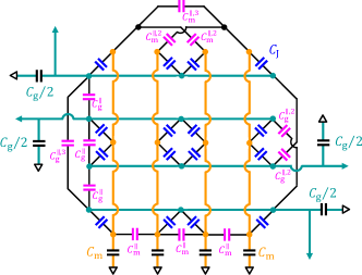
Figure 8: Illustration of the capacitances present in a single site of the JJ array. Green thick lines are gauge wires, and orange thick lines are matter wires.

In section V.1 we discussed the requirements to realize the magnetic potential of Eqs. (4) and (4b) which exhibits combinatorial gauge symmetry. The question also arises, however, whether this symmetry can be broken in any important ways by the electrostatic part of the Hamiltonian, Eq. (2). This corresponds to non-invariance of $\mathbf{C}^{-1}$ under permutations of the matter wires within each site. Referring to Fig. 8: while it is reasonable to assume that the self-capacitance of the matter wires $C_{\rm m}$ can be made symmetric within each site, the parasitic capacitances between matter wires $C_{\rm m}^{||}$, $C_{\rm m}^{||,2}$, and $C_{\rm m}^{||,3}$ will not naturally be equal, and therefore will break the symmetry.

However, these parasitic capacitances do not appear in the tunneling energy to leading order Kerman , so that from the perspective of low-energy, static emulation of the toric code, we are justified in neglecting this small symmetry breaking. That said, it is still possible that these effects could become important when the system’s dynamic response to noise is considered, in the context of topological protection of quantum information. Should this turn out to be the case, we show schematically in Figure 9 that with appropriate electrostatic design, the parasitic capacitances could be symmetrized so as to null out the combinatorial symmetry-breaking.

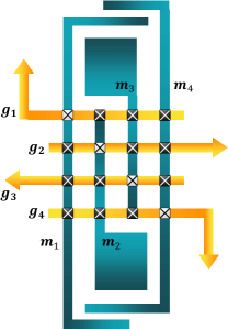
Figure 9: Schematic for restoring combinatorial symmetry to the inverse capacitance matrix of a site.

Another effect in the electrostatic Hamiltonian which could break the combinatorial symmetry would be a spurious asymmetry in the capacitances across the DC SQUID coupling elements between matter and gauge wires (arising from fabrication process variation of junction sizes). Although such imperfections contribute in leading order to the diagonal elements of $\mathbf{C}^{-1}$, the resulting breaking of the symmetry can be expected to be quite small, for two reasons. First, unlike the fabrication variations in the Josephson energy, which depend exponentially on the dielectric barrier thickness, junction capacitance $C_{\rm J}$ depends only inversely on this thickness, so that the resulting variations are even smaller than that observed in $J$. Second, the numerical coefficient of the linear correction term breaking the symmetry is small (1/8 in the simplest circuit model Kerman ), pushing the resulting expected fractional variation between diagonal charging energy terms to the $\sim 10^{-3}$ level for junction size uniformity of a few percentNiedzielski et al. (2019).

Summary

We have proposed a superconducting quantum circuit based on Josephson junction arrays that realizes combinatorial gauge symmetry. This symmetry is both local and exact and leads to interesting loop phases with topological order. We have argued that the model admits a gapped quantum topological phase which should be stable for a wide range of parameters. The general framework laid out here offers a promising path to engineering exotic many-body states in the laboratory and to realizing a platform for topological quantum computation.

Appendix A Plaquette operators

The local combinatorial gauge symmetry allows us to construct local conserved quantities – plaquette operators on each plaquette $p$:

$$G_{p}=\prod_{s\in p}{\mathcal{L}}^{(\hat{a})}_{s}\prod_{i\in p}{\mathcal{R}}^{(\hat{b})}_{i}~{}.$$ (24)

The product of the ${\mathcal{R}}^{(\hat{b})}_{i}$ around the plaquette flips both legs at each corner site $s$. An example is shown in the inset of Fig. 1(c). $\mathcal{L}^{(\hat{a})}_{s}$ is the companion operator that permutes and flips the matter fields at each corner site per Eqs. (6) and  (9). Any two $L$ matrices commute and therefore the plaquette operators do as well, $[G_{p},G_{p^{\prime}}]=0$. Finally, gauge symmetry guarantees that $G_{p}$ is conserved for all $p$: $[H,G_{p}]=0$.

Appendix B Loop fugacity of continuous variables

Here we clarify the argument in the main text regarding the zero temperature partition function of the $U(1)$ loop component. Recall that our phases are defined mod $\pi$ and not mod $2\pi$, but the difference is simply a factor of 1/2 in the fugacity, so below we present the argument for the mod $2\pi$ case and return to this issue at the end of this appendix section.

Consider a loop $\mathcal{C}$ with length $p$, $p$ continuous variables $\theta_{i},i=1,\dots p$, and a Boltzmann factor that penalizes configurations where consecutive variables are different ($\theta_{p}$ is consecutive to $\theta_{1}$). We can write the contribution of this loop to the partition function as

$$Z_{\mathcal{C}}=\int_{0}^{2\pi}\frac{d\theta_{1}}{2\pi}\,\frac{d\theta_{2}}{2\pi}\dots\dots\frac{d\theta_{p}}{2\pi}\;e^{-K[1-\cos(\theta_{1}-\theta_{2})]}\;e^{-K[1-\cos(\theta_{2}-\theta_{3})]}\;\dots e^{-K[1-\cos(\theta_{p-1}-\theta_{p})]}\;e^{-K[1-\cos(\theta_{p}-\theta_{1})]}\;\;,$$ (25)

where the Boltzmann factor that imposes the constraint is $e^{-K[1-\cos(\theta_{i}-\theta_{i+1})]}$. The overall ground state energy has been left out because it is identical for all configurations on the lattice. As $K\to\infty$ we can replace the factors by Gaussian approximations:

$$Z_{\mathcal{C}} \approx\int_{0}^{2\pi}\frac{d\theta_{1}}{2\pi}\,\frac{d\theta_{2}}{2\pi}\dots\dots\frac{d\theta_{p}}{2\pi}\;e^{-\frac{K}{2}(\theta_{1}-\theta_{2})^{2}}\;e^{-\frac{K}{2}(\theta_{2}-\theta_{3})^{2}}\;\dots e^{-\frac{K}{2}(\theta_{p-1}-\theta_{p})^{2}}\;e^{-\frac{K}{2}(\theta_{p}-\theta_{1})^{2}}\;$$

$$\approx\int_{0}^{2\pi}\frac{d\theta_{1}}{2\pi}\,\frac{d\theta_{2}}{2\pi}\dots\dots\frac{d\theta_{p}}{2\pi}\;[\sqrt{\frac{2\pi}{K}}\;\delta(\theta_{1}-\theta_{2})]\;[\sqrt{\frac{2\pi}{K}}\;\delta(\theta_{2}-\theta_{3})]\;\dots[\sqrt{\frac{2\pi}{K}}\;\delta(\theta_{p-1}-\theta_{p})]\;e^{-\frac{K}{2}(\theta_{p}-\theta_{1})^{2}}\;$$

$$=\left(\sqrt{\frac{1}{2\pi K}}\right)^{p-1}\int_{0}^{2\pi}\frac{d\theta_{1}}{2\pi}\;,$$ (26)

where we replaced the Gaussian approximations by the delta functions for all links with the exception of the last because it is automatically enforced by the other $p-1$ constraints. The one less power of the factor $\sqrt{1/2\pi K}$ has its origin in the last link, which closes the loop.

In a fully packed lattice model, each term in the partition function is an integral over $n_{B}$ bonds, where $n_{B}$ is the total number of bonds on the lattice. Therefore each loop configuration will contribute the factor $\left(\sqrt{1/2\pi K}\right)^{n_{B}-n_{\ell}}$, where $n_{\ell}$ is the number of loops in the configuration. Ignoring the overall factor for number of bonds, we can identify the loop fugacity $\lambda$ as

$$\lambda=\sqrt{2\pi K}\to\infty\quad{\rm if}\;K\to\infty\;.$$ (27)

We can think of this result formally as the integration over one redundant delta function since only $p-1$ delta functions are required to enforce a constraint around a loop with perimeter $p$; the remaining delta function is evaluated at 0, giving the value “$\delta(0)$” to the fugacity.

More intuitively, the result follows the simple expectation that we have a continuous phases (infinitely many colors) associated with each loop.

We now return to the issue that our phases are defined mod $\pi$ and not mod $2\pi$. Changing all the $\int_{0}^{2\pi}\frac{d\theta_{i}}{2\pi}\to\int_{0}^{\pi}\frac{d\theta_{i}}{\pi}$ in Eq. (B) changes the result for the fugacity by a factor of 1/2, i.e., we replace the $\lambda$ found above by $\lambda/2$. Of course, none of the discussion above changes as $\lambda\to\infty$. Nonetheless, this factor reinforces the simple intuitive interpretation of the continuous angles representing infinitely many colors: half the continuous angles correspond to half the infinitely many colors, as expressed by the scaling of $\lambda$ by 1/2.

Appendix C “WXY Model”: limit of small capacitances in all wires

We present another limit of the superconducting wire array that is equivalent to a spin-1/2 system with two-body interactions and an exact ${\mathbb{Z}}_{2}$ gauge symmetry. Consider the limit where both the matter and gauge capacitances are small, and voltage biases are tuned so two nearly degenerate charge states are favored in each matter and gauge wire. In this limit, we reach an interesting spin model that could potentially have a gap of order $E_{J}$, as we argue below.

In the limit when the wires become two-level systems, we can deploy spin-1/2 raising and lowering operators via the replacements $e^{\pm\mathrm{i}\,\phi_{n}}\to\mu^{\pm}_{n}$ and $e^{\pm\mathrm{i}\,\theta_{i}}\to\sigma^{\pm}_{i}$. In terms of combinatorial gauge symmetry we can identify the small capacitance version of Eq.(10):

$$\hat{a}_{n}=\mu^{-}_{n}\quad \text{and}\quad\hat{b}_{i}=\sigma^{-}_{i}$$

$$U^{(L)}_{n}=e^{\mathrm{i}\frac{\pi}{2}\,\mu^{\rm z}_{n}}=\mathrm{i}\mu^{\rm z}_{n}\quad \text{and}\quad U^{(R)}_{i}=e^{\mathrm{i}\frac{\pi}{2}\,\sigma^{\rm z}_{i}}=\mathrm{i}\sigma^{\rm z}_{i}\;.$$ (28)

The Hamiltonian takes the form reminiscent of the standard quantum XY-model, but again with the crucial Hadamard symmetry:

$$H_{J}=-J\;\sum_{s}\sum_{n,i\in s}W_{ni}\;\left(\mu^{\rm x}_{n}\;\sigma^{\rm x}_{i}+\mu^{\rm y}_{n}\;\sigma^{\rm y}_{i}\right)\;.$$ (29)

We refer to this model as “WXY”. If the wires are biased slightly away from the degenerate point, kinetic terms of the form $\mu^{\rm z}_{n}$ and $\sigma^{\rm z}_{i}$ appear. These terms commute with both $U^{(L)}_{n}$ and $U^{(R)}_{i}$, and if the couplings are uniform they satisfy the permutation part of the combinatorial gauge symmetry. However, these kinetic terms are not required as quantum dynamics is present at the outset in the WXY-model of Eq. (29).

Is its low-energy spectrum gapped? Answering this question is outside the scope of this work, and may require a detailed numerical study. [We note that the quantum WXY-model of Eq. (29) has a sign problem, so numerical studies would require methods such as the Density Matrix Renormalization Group (DMRG).] If the model does turn out to be gapped, the only energy scale in the Hamiltonian is $J$, and therefore such gap would be rather large. Given that the model has an exact ${\mathbb{Z}}_{2}$ symmetry, we believe it is an interesting spin model to study even if it is gapless.

Appendix D Capacitance matrix

$$\mathbf{C}_{\rm s}=\begin{pmatrix}C_{\rm m}+4C_{\rm J}+C_{\rm m}^{||}&-C_{\rm m}^{||}&-C_{\rm m}^{||,2}&-C_{\rm m}^{||,3}&-C_{\rm J}&-C_{\rm J}&-C_{\rm J}&-C_{\rm J}\\ +C_{\rm m}^{||,2}+C_{\rm m}^{||,3}&\\ \\ -C_{\rm m}^{||}&C_{\rm m}+4C_{\rm J}&-C_{\rm m}^{||}&-C_{\rm m}^{||,2}&-C_{\rm J}&-C_{\rm J}&-C_{\rm J}&-C_{\rm J}\\ &+2C_{\rm m}^{||}+C_{\rm m}^{||,2}\\ \\ -C_{\rm m}^{||,2}&-C_{\rm m}^{||}&C_{\rm m}+4C_{\rm J}&-C_{\rm m}^{||}&-C_{\rm J}&-C_{\rm J}&-C_{\rm J}&-C_{\rm J}\\ &&+2C_{\rm m}^{||}+C_{\rm m}^{||,2}\\ \\ -C_{\rm m}^{||,3}&-C_{\rm m}^{||,2}&-C_{\rm m}^{||}&C_{\rm m}+4C_{\rm J}+C_{\rm m}^{||}&-C_{\rm J}&-C_{\rm J}&-C_{\rm J}&-C_{\rm J}\\ &&&+C_{\rm m}^{||,2}+C_{\rm m}^{||,3}&\\ \\ -C_{\rm J}&-C_{\rm J}&-C_{\rm J}&-C_{\rm J}&C_{\rm g}/2+4C_{\rm J}+C_{\rm g}^{||}&-C_{\rm g}^{||}&-C_{\rm g}^{||,2}&-C_{\rm g}^{||,3}\\ &&&&+C_{\rm g}^{||,2}+C_{\rm g}^{||,3}&\\ \\ -C_{\rm J}&-C_{\rm J}&-C_{\rm J}&-C_{\rm J}&-C_{\rm g}^{||}&C_{\rm g}/2+4C_{\rm J}&-C_{\rm g}^{||}&-C_{\rm g}^{||,2}\\ &&&&&+2C_{\rm g}^{||}+C_{\rm g}^{||,2}\\ \\ -C_{\rm J}&-C_{\rm J}&-C_{\rm J}&-C_{\rm J}&-C_{\rm g}^{||,2}&-C_{\rm g}^{||}&C_{\rm g}/2+4C_{\rm J}&-C_{\rm g}^{||}\\ &&&&&&+2C_{\rm g}^{||}+C_{\rm g}^{||,2}\\ \\ -C_{\rm J}&-C_{\rm J}&-C_{\rm J}&-C_{\rm J}&-C_{\rm g}^{||,3}&-C_{\rm g}^{||,2}&-C_{\rm g}^{||}&C_{\rm g}/2+4C_{\rm J}+C_{\rm g}^{||}\\ &&&&&&&+C_{\rm g}^{||,2}+C_{\rm g}^{||,3}&\\ \\ \end{pmatrix}$$ (30)

Appendix E Magnetic potential of asymmetric DC SQUID coupling elements

The magnetic potential energy of the asymmetric DC SQUID in Fig. 7(b) can be written (taking $L_{\rm w}=L_{\rm t}=L$ and $J_{\rm t}/J_{\rm w}\equiv d_{J}\ll 1$):

$$\frac{U}{J_{\rm w}}=-\cos{\left(\phi_{n}-\theta_{i}-\varphi_{\rm ow}+2\pi\frac{\Phi_{\rm w}}{\Phi_{0}}\right)}$$

$$-d_{J}\cos{\left(\phi_{n}-\theta_{i}-\varphi_{\rm ot}+2\pi\frac{\Phi_{\rm t}}{\Phi_{0}}\right)}$$

$$+\frac{1}{2e_{LJ}}\left(\varphi_{\rm ow}^{2}+\varphi_{\rm ot}^{2}\right)$$ (31a)

where we have defined the displaced oscillator coordinates:

$$\varphi_{\rm ow}\equiv\varphi_{\rm w}-\theta_{i}-2\pi\frac{\Phi_{\rm w}}{\Phi_{0}}$$

$$\varphi_{\rm ot}\equiv\varphi_{\rm t}-\theta_{i}-2\pi\frac{\Phi_{\rm t}}{\Phi_{0}}$$ (31b)

and the ratio between Josephson and linear inductive energy:

$$e_{LJ}\equiv\frac{4\pi^{2}L}{\Phi_{0}^{2}}J_{\rm w}$$ (31c)

We can simplify Eq. 31a by approximating the two (high-frequency) oscillator mode coordinates by the values which minimize the inductive energy with respect to each coordinate. Substituting these values for $\varphi_{ow}$ and $\varphi_{ot}$ back into Eq. 31a, we obtain, to second order in $d_{L}$ and $e_{LJ}$:

$$\frac{U}{J_{\rm w}}\approx-\left(1-\frac{e_{LJ}^{2}}{8}\right)\cos{\left(\phi_{n}-\theta_{i}+2\pi\frac{\Phi_{\rm w}}{\Phi_{0}}\right)}$$

$$-d_{J}\cos{\left(\phi_{n}-\theta_{i}+2\pi\frac{\Phi_{\rm t}}{\Phi_{0}}\right)}$$

$$+\frac{e_{LJ}}{4}\cos{\left[2\left(\phi_{n}-\theta_{i}+2\pi\frac{\Phi_{\rm w}}{\Phi_{0}}\right)\right]}$$

$$-\frac{e_{LJ}^{2}}{8}\cos{\left[3\left(\phi_{n}-\theta_{i}+2\pi\frac{\Phi_{\rm w}}{\Phi_{0}}\right)\right]}$$ (32)

The first two terms of this result correspond to the phasor diagram of Fig. 7(c), with a renormalization of the effective Josephson energy $J_{\rm w}$ due to the finite loop inductance.

The last two terms are first and second-order distortions of the effective Josephson potential by the loop inductance, which can be viewed as weak two- and three-Cooper-pair tunneling terms. Although the effect of these terms on the phases of our model are not yet understood, they can be made small via the parameter $e_{LJ}$. The extent to which this parameter can be reduced will be determined by how small the loop inductances and Josephson energies can be made, while retaining the ability to provide sufficient bias flux and keeping the Josephson energy scale large enough compared to $k_{B}T$. To get a rough estimate of this quantity, if we take the reasonable values: $J_{\rm w}\sim k_{B}\times 1$K, and $L_{w}\sim 10$pH, we obtain: $e_{LJ}\sim 10^{-4}$.

References

- Devoret et al. (2004) M. H. Devoret, A. Wallraff, and J. M. Martinis, “Superconducting qubits: A short review,” (2004), arXiv:cond-mat/0411174 .
- King et al. (2018) A. D. King, J. Carrasquilla, J. Raymond, I. Ozfidan, E. Andriyash, A. Berkley, M. Reis, T. Lanting, R. Harris, F. Altomare, K. Boothby, P. I. Bunyk, C. Enderud, A. Frechette, E. Hoskinson, N. Ladizinsky, T. Oh, G. Poulin-Lamarre, C. Rich, Y. Sato, A. Y. Smirnov, L. J. Swenson, M. H. Volkmann, J. Whittaker, J. Yao, E. Ladizinsky, M. W. Johnson, J. Hilton, and M. H. Amin, “Observation of topological phenomena in a programmable lattice of 1,800 qubits,” Nature 560, 456–460 (2018).
- Arute et al. (2019) F. Arute, K. Arya, R. Babbush, D. Bacon, J. C. Bardin, R. Barends, R. Biswas, S. Boixo, F. G. S. L. Brandao, D. A. Buell, and et al., “Quantum supremacy using a programmable superconducting processor,” Nature 574, 505–510 (2019).
- Kjaergaard et al. (2020) M. Kjaergaard, M. E. Schwartz, J. Braumüller, P. Krantz, J. I.-J. Wang, S. Gustavsson, and W. D. Oliver, “Superconducting qubits: Current state of play,” Annual Review of Condensed Matter Physics 11, 369–395 (2020), https://doi.org/10.1146/annurev-conmatphys-031119-050605 .
- Resnick et al. (1981) D. J. Resnick, J. C. Garland, J. T. Boyd, S. Shoemaker, and R. S. Newrock, “Kosterlitz-Thouless transition in proximity-coupled superconducting arrays,” Phys. Rev. Lett. 47, 1542–1545 (1981).
- Chamon et al. (2020) C. Chamon, D. Green, and Z.-C. Yang, “Constructing quantum spin liquids using combinatorial gauge symmetry,” Phys. Rev. Lett. 125, 067203 (2020).
- Wen (1990) X. G. Wen, “Topological Orders in Rigid States,” International Journal of Modern Physics B 04, 239–271 (1990).
- Savary and Balents (2016) L. Savary and L. Balents, “Quantum spin liquids: a review,” Reports on Progress in Physics 80, 016502 (2016).
- Kitaev (2006) A. Kitaev, “Anyons in an exactly solved model and beyond,” Ann. Phys. 321, 2–111 (2006).
- Jackeli and Khaliullin (2009) G. Jackeli and G. Khaliullin, “Mott insulators in the strong spin-orbit coupling limit: From Heisenberg to a quantum compass and Kitaev models,” Phys. Rev. Lett. 102, 017205 (2009).
- Ioffe et al. (2002) L. B. Ioffe, M. V. Feigel’man, A. Ioselevich, D. Ivanov, M. Troyer, and G. Blatter, “Topologically protected quantum bits using Josephson junction arrays,” Nature 415, 503–506 (2002).
- Ioffe and Feigel’man (2002) L. B. Ioffe and M. V. Feigel’man, “Possible realization of an ideal quantum computer in Josephson junction array,” Phys. Rev. B 66, 224503 (2002).
- Douçot et al. (2005) B. Douçot, M. V. Feigel’man, L. B. Ioffe, and A. S. Ioselevich, “Protected qubits and Chern-Simons theories in Josephson junction arrays,” Phys. Rev. B 71, 024505 (2005).
- Douçot et al. (2003) B. Douçot, M. V. Feigel’man, and L. B. Ioffe, “Topological order in the insulating Josephson junction array,” Phys. Rev. Lett. 90, 107003 (2003).
- Gladchenko et al. (2009) S. Gladchenko, D. Olaya, E. Dupont-Ferrier, B. Douçot, L. B. Ioffe, and M. E. Gershenson, “Superconducting nanocircuits for topologically protected qubits,” Nature Physics 5, 48–53 (2009).
- Douçot and Ioffe (2012) B. Douçot and L. B. Ioffe, “Physical implementation of protected qubits,” Reports on Progress in Physics 75, 072001 (2012).
- Chayes et al. (2000) L. Chayes, L. P. Pryadko, and K. Shtengel, “Intersecting loop models on Zd: rigorous results,” Nuclear Physics B 570, 590 – 614 (2000).
- Read and Saleur (2003) N. Read and H. Saleur, “Dense loops, supersymmetry, and goldstone phases in two dimensions,” Physical review letters 90, 090601 (2003).
- Blöte et al. (2012) H. W. J. Blöte, Y. Wang, and W. Guo, “The completely packed o(n) loop model on the square lattice,” Journal of Physics A: Mathematical and Theoretical 45, 494016 (2012).
- Nahum et al. (2013) A. Nahum, P. Serna, A. M. Somoza, and M. Ortuño, “Loop models with crossings,” Phys. Rev. B 87, 184204 (2013).
- Castelnovo and Chamon (2007) C. Castelnovo and C. Chamon, “Topological order and topological entropy in classical systems,” Phys. Rev. B 76, 174416 (2007).
- (22) C.C. and D.G. thank Garry Goldstein for alerting us that dimensional reduction leads to an effective barrier and suggesting a simple physical argument for the scaling of the gap in a special case.
- (23) A. J. Kerman, unpublished.
- Geerligs et al. (1990) L. J. Geerligs, V. F. Anderegg, and J. E. Mooij, “Tunneling time and offset charging in small tunnel junctions,” Physica B: Condensed Matter 165–166, 973–974 (1990).
- Kuzmin et al. (1989) L. S. Kuzmin, P. Delsing, T. Claeson, and K. K. Likharev, “Single-electron charging effects in one-dimensional arrays of ultrasmall tunnel junctions,” Phys. Rev. Lett. 62, 2539–2542 (1989).
- Zimmerli et al. (1992) G. Zimmerli, T. M. Eiles, R. L. Kautz, and J. M. Martinis, “Noise in the coulomb blockade electrometer,” Applied Physics Letters 61, 237–239 (1992).
- Ithier et al. (2005) G. Ithier, E. Collin, P. Joyez, P. J. Meeson, D. Vion, D. Esteve, F. Chiarello, A. Shnirman, Y. Makhlin, J. Schriefl, and G. Schön, “Decoherence in a superconducting quantum bit circuit,” Phys. Rev. B 72, 134519 (2005).
- Yoshihara et al. (2006) F. Yoshihara, K. Harrabi, A. O. Niskanen, Y. Nakamura, and J. S. Tsai, “Decoherence of flux qubits due to flux noise,” Phys. Rev. Lett. 97, 167001 (2006).
- Bylander et al. (2011) J. Bylander, S. Gustavsson, F. Yan, F. Yoshihara, K. Harrabi, G. Fitch, D. G. Cory, Y. Nakamura, J.-S. Tsai, and W. D. Oliver, “Noise spectroscopy through dynamical decoupling with a superconducting flux qubit,” Nature Physics 7, 565–570 (2011).
- Yan et al. (2016) F. Yan, S. Gustavsson, A. Kamal, J. Birenbaum, A. P. Sears, D. Hover, T. J. Gudmundsen, D. Rosenberg, G. Samach, S. Weber, J. L. Yoder, T. P. Orlando, J. Clarke, A. J. Kerman, and W. D. Oliver, “The flux qubit revisited to enhance coherence and reproducibility,” Nature Communications 7, 12964 (2016).
- Niedzielski et al. (2019) B. M. Niedzielski, D. K. Kim, M. E. Schwartz, D. Rosenberg, G. Calusine, R. Das, A. J. Melville, J. Plant, L. Racz, J. L. Yoder, D. Ruth-Yost, and W. D. Oliver, “Silicon hard-stop spacers for 3d integration of superconducting qubits,” in 2019 IEEE International Electron Devices Meeting (IEDM) (2019) pp. 31.3.1–31.3.4.
- Frolov et al. (2004) S. M. Frolov, D. J. Van Harlingen, V. A. Oboznov, V. V. Bolginov, and V. V. Ryazanov, “Measurement of the current-phase relation of superconductor/ferromagnet/superconductor josephson junctions,” Phys. Rev. B 70, 144505 (2004).
- Yamashita et al. (2005) T. Yamashita, K. Tanikawa, S. Takahashi, and S. Maekawa, “Superconducting qubit with a ferromagnetic josephson junction,” Phys. Rev. Lett. 95, 097001 (2005).
- Feofanov et al. (2010) A. K. Feofanov, V. A. Oboznov, V. V. Bol’ginov, J. Lisenfeld, S. Poletto, V. V. Ryazanov, A. N. Rossolenko, M. Khabipov, D. Balashov, A. B. Zorin, P. N. Dmitriev, V. P. Koshelets, and A. V. Ustinov, “Implementation of superconductor/ferromagnet/superconductor -shifters in superconducting digital and quantum circuits,” Nature Physics , 593–597 (2010).