The ASAS-SN Catalog of Variable Stars IX: The Spectroscopic Properties of Galactic Variable Stars

Abstract

The All-Sky Automated Survey for Supernovae (ASAS-SN) provides long baseline (${\sim}4$ yrs) $V-$band light curves for sources brighter than V$\lesssim 17$ mag across the whole sky. We produced V-band light curves for a total of ${\sim}61.5$ million sources and systematically searched these sources for variability. We identified ${\sim}426,000$ variables, including ${\sim}219,000$ new discoveries. Most (${\sim}74\%$) of our discoveries are in the Southern hemisphere. Here we use spectroscopic information from LAMOST, GALAH, RAVE, and APOGEE to study the physical and chemical properties of these variables. We find that metal-poor eclipsing binaries have orbital periods that are shorter than metal-rich systems at fixed temperature. We identified rotational variables on the main-sequence, red giant branch and the red clump. A substantial fraction (${\gtrsim}80\%$) of the rotating giants have large $v_{\rm rot}$ or large NUV excesses also indicative of fast rotation. The rotational variables have unusual abundances suggestive of analysis problems. Semi-regular variables tend to be lower metallicity ($\rm[Fe/H]{\sim}-0.5$) than most giant stars. We find that the APOGEE DR16 temperatures of oxygen-rich semi-regular variables are strongly correlated with the $W_{RP}-W_{JK}$ color index for $\rm T_{eff}\lesssim 3800$ K. Using abundance measurements from APOGEE DR16, we find evidence for Mg and N enrichment in the semi-regular variables. We find that the Aluminum abundances of the semi-regular variables are strongly correlated with the pulsation period, where the variables with $\rm P\gtrsim 60$ days are significantly depleted in Al.

1 Introduction

Variable stars are useful astrophysical tools that can be used to study the lives and deaths of stars. Pulsating variables, including Cepheids, RR Lyrae stars and Mira variables are used as distance indicators as they follow distinct period-luminosity relationships (e.g., Leavitt 1908; Matsunaga et al. 2006; Beaton et al. 2018; Whitelock et al. 2008, and references therein). Eclipsing binary stars allow for the derivation of dynamical information and fundamental stellar parameters, including the masses and radii of the stars (Torres et al., 2010). The precise measurements afforded by eclipsing binaries allow for tests of stellar theory across the Hertzsprung-Russell diagram. Variable stars are also used to study stellar populations and Galactic structure (Mateu & Vivas, 2018; Matsunaga, 2018; Feast & Whitelock, 2014).

Modern large scale sky surveys such as the All-Sky Automated Survey (ASAS; Pojmanski 2002), the All-Sky Automated Survey for SuperNovae (ASAS-SN, Shappee et al. 2014; Kochanek et al. 2017; Jayasinghe et al. 2018), the Optical Gravitational Lensing Experiment (OGLE; Udalski 2003), the Northern Sky Variability Survey (NSVS; Woźniak et al. 2004), MACHO (Alcock et al., 1997), EROS (Derue et al., 2002), the Catalina Real-Time Transient Survey (CRTS; Drake et al. 2014), the Asteroid Terrestrial-impact Last Alert System (ATLAS; Tonry et al. 2018a; Heinze et al. 2018), Gaia (Gaia Collaboration et al., 2018; Holl et al., 2018; Gaia Collaboration et al., 2019), and the Zwicky Transient Facility (Bellm et al., 2019; Chen et al., 2020) have revolutionized the study of stellar variability. Amateur astronomers have also contributed to these discoveries over the years. As of May 2020, the International Variable Stars Index (VSX,Watson et al. 2006) hosted by the American Association of Variable Star Observers (AAVSO) lists ${\sim}1.4\times 10^{6}$ variable stars.

In addition to these modern photometric surveys, large-scale wide-field spectroscopic surveys such as the Apache Point Observatory Galactic Evolution Experiement (APOGEE; Gunn et al. 2006; Blanton et al. 2017; Wilson et al. 2019), Large Sky Area Multi-Object Fibre Spectroscopic Telescope (LAMOST Cui et al. 2012), GALactic Archaeology with HERMES (GALAH; De Silva et al. 2015; Buder et al. 2018) and the RAdial Velocity Experiment (RAVE;Casey et al. 2017) have been making medium/high resolution spectroscopic observations of millions of Galactic stars. Spectroscopic observations of Galactic stars are invaluable for deciphering the chemical evolution of our Galaxy (see for e.g.,Weinberg et al. 2019; Griffith et al. 2019), and for evolved stars they also provide clues to understanding chemical enrichment caused by dredge up episodes (see for e.g., Salaris et al. 2015; Shetrone et al. 2019. Variable stars that have both extensive time-series data and spectroscopic observations will allow for the study of stellar evolution to great detail.

ASAS-SN monitored the visible sky to a depth of $V\lesssim 17$ mag with a cadence of 2-3 days using two units in Chile and Hawaii each with 4 telescopes from 2014-2018. Since then, ASAS-SN has expanded to 5 units with 20 telescopes and is currently monitoring the sky in the $g$-band to a depth of $g\lesssim 18.5$ mag with a cadence of $\sim 1$ day. The ASAS-SN telescopes are hosted by the Las Cumbres Observatory (LCO; Brown et al. 2013) in Hawaii, Chile, Texas and South Africa. The primary focus of ASAS-SN is the detection of bright supernovae and other transients (e.g., tidal disruption events, cataclysmic variables, AGN flares, stellar flares, etc.) with minimal bias (e.g., Holoien et al. 2014, 2016, 2017), but its excellent baseline and all-sky coverage allows for the characterization of stellar variability across the whole sky.

In Paper I (Jayasinghe et al., 2018), we discovered ${\sim}66,000$ new variables that were flagged during the search for supernovae, most of which are located in regions that were not well-sampled by previous surveys. In Paper II (Jayasinghe et al., 2019b), we homogeneously analyzed ${\sim}412,000$ known variables from the VSX catalog, and developed a versatile random forest variability classifier utilizing the ASAS-SN V-band light curves and data from external catalogues. As data from The Transiting Exoplanet Survey Satellite (TESS; Ricker et al. 2015) became available, we have explored the synergy between the two surveys. In Paper III (Jayasinghe et al., 2019a), we characterized the variability of ${\sim}1.3$ million sources within 18 deg of the Southern Ecliptic Pole towards the TESS continuous viewing zone and identified ${\sim}11,700$ variables, including ${\sim}7,000$ new discoveries. We have also explored the synergy between ASAS-SN and large scale spectroscopic surveys using data from APOGEE (Holtzman et al., 2015) with the discovery of the first likely non-interacting binary composed of a black hole with a field red giant (Thompson et al., 2019) and the identification of 1924 APOGEE stars as periodic variables in Paper IV (Pawlak et al., 2019). In Paper V, we systematically searched for variable sources with $V<17$ mag in the southern hemisphere and identified ${\sim}220,000$ variable sources, of which ${\sim}88,300$ were new discoveries (Jayasinghe et al., 2019c). In Paper VI, we derived period–luminosity relationships for $\delta$ Scuti stars (Jayasinghe et al., 2020b). We studied contact binaries in Paper VII (Jayasinghe et al., 2020a). In Paper VIII, we identified 11 new “dipper” stars in the Lupus star forming region (Bredall et al., 2020).

Here, we summarize the results of our $V$-band variability search based on ${\sim}61.5$ million ASAS-SN light curves of sources from the AAVSO Photometric All-Sky Survey (APASS; Henden et al. 2015) DR9 catalog with $V<17$ mag and the ATLAS All-Sky Stellar Reference Catalog (refcat2, Tonry et al. 2018b) catalog with $g<17$ mag. In this work, we describe our $V$-band variability catalog of ${\sim}426,000$ variable sources, of which ${\sim}219,000$ are new discoveries. In Section $\S 2$, we discuss the ASAS-SN observations, our variable star identification and classification procedure and summarize the final $V$-band catalog. Section $\S 3$ discusses the cross-matches made to various spectroscopic catalogs and the general spectroscopic properties of the ASAS-SN variable stars. In Section $\S 4$, we discuss the eclipsing binaries, rotational variables and semi-regular variables in greater depth and present a summary of our work in Section $\S 5$.

2 The ASAS-SN $V$-band Catalog of Variable Stars

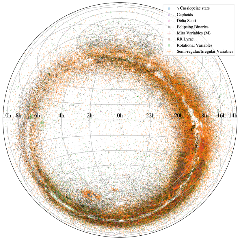
Figure 1: Projected distribution of the $\sim 219,200$ new ASAS-SN discoveries in Equatorial coordinates (Lambert projection). The points are colored by the variability type.

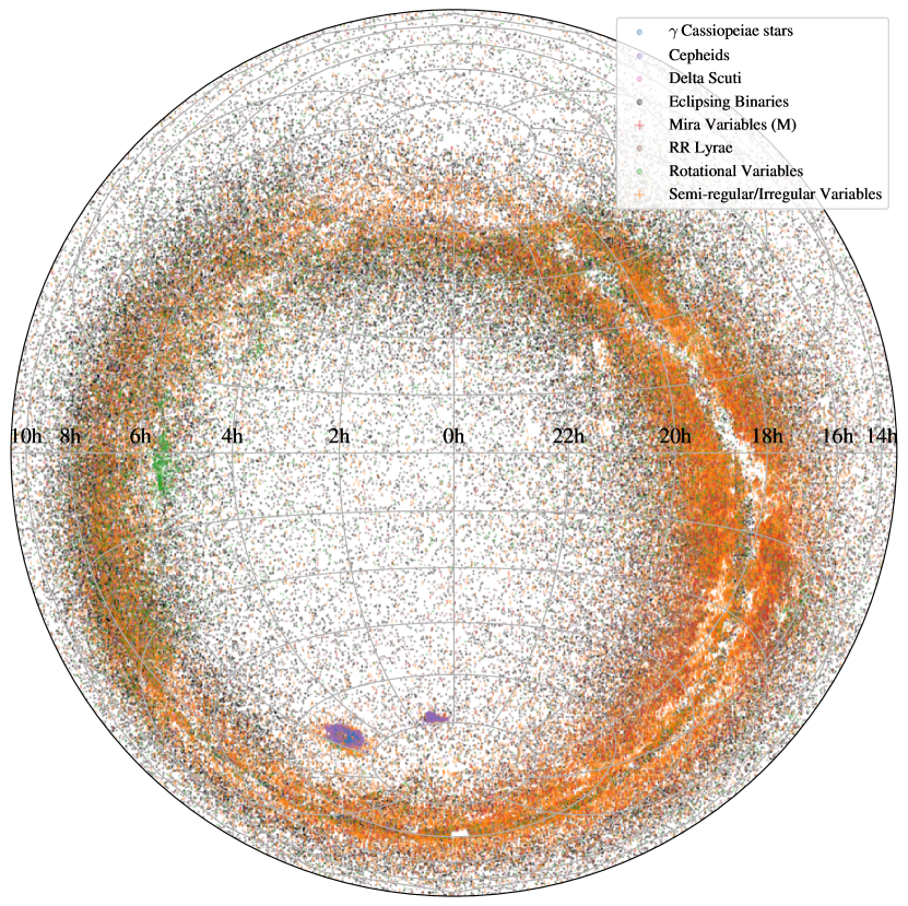
Figure 2: Projected distribution of the $\sim 207,200$ known variable stars recovered through ASAS-SN in Equatorial coordinates (Lambert projection). The points are colored by the variability type.

The ASAS-SN V-band observations used in this work were made by the “Brutus" (Haleakala, Hawaii) and “Cassius" (CTIO, Chile) quadruple telescopes between 2013 and 2018. Each ASAS-SN V-band field is observed to a depth of $V\lesssim 17$ mag. The field of view of an ASAS-SN camera is 4.5 deg², the pixel scale is 8$\aas@@fstack{\prime\prime}$0 and the FWHM is typically ${\sim}2$ pixels. ASAS-SN tends to saturate at ${\sim}10-11$ mag, but we attempt to correct the light curves of saturated sources for bleed trails (see Kochanek et al. 2017). The V-band light curves were extracted as described in Jayasinghe et al. (2018) using image subtraction (Alard & Lupton, 1998; Alard, 2000) and aperture photometry on the subtracted images with a 2 pixel radius aperture. We corrected the zero point offsets between the different cameras as described in Jayasinghe et al. (2018). The photometric errors were recalculated as described in Jayasinghe et al. (2019a).

As we did in Paper V, we started with the APASS DR9 catalog (Henden et al., 2015) as our input source catalog for the northern hemisphere. We selected ${\sim}23.1$M APASS sources with $V<17$ mag in the northern hemisphere ($\delta>0$ deg). However, there are regions towards the Galactic plane that are missing in the APASS DR9 catalog (Henden et al., 2015; Marrese et al., 2019). To address the issue of incomplete sky coverage, we used the refcat2 catalog (Tonry et al., 2018b) to produce light curves for the sources missing from APASS DR9. From the refcat2 catalog, we selected ${\sim}7.1$M sources with r1$>30"$ and $G<17$ mag, where r1 is the radius at which the cumulative $G$ flux in the aperture exceeds the flux of the source being considered and is a measure of blending around a star. We use this cut in r1 to reduce the number of heavily blended sources. This does bias the selected refcat2 sources towards more isolated stars, and will reduce the completeness of the catalog, especially towards the Galactic plane. In total, we produced ${\sim}61.5$M $V$-band light curves. The V-band light curves of all ${\sim}61.5$M sources are available online at the ASAS-SN Photometry Database (https://asas-sn.osu.edu/photometry).

We applied the trained random forest classifier from Jayasinghe et al. (2019c) to identify candidate variables. From this sample, blended sources were identified and removed as described in Jayasinghe et al. (2019c). Following these procedures, we used the variability classifier implemented in Jayasinghe et al. (2019b), which consists of a random forest classifier plus several refinement steps, in order to classify the candidate variables. We applied additional quality checks to improve the purity of our catalog (summarized in Table 4 from Jayasinghe et al. 2019c). Peak-to-peak variability amplitudes were estimated by fitting a random forest regression model to the light curves (Jayasinghe et al., 2019c). We previously noted that light curves that are contaminated by systematics tend to be classified as irregular or generic variables. Thus, we visually reviewed all the sources that were classified as L, VAR, GCAS, or YSO to improve the purity of our catalog. Following this, we identified ${\sim}124,000$ and ${\sim}40,000$ variables among the northern APASS sources and the refcat2 sources, respectively. As described in Jayasinghe et al. (2019c), we cross-matched these variables to the various catalogs of known variable stars. Following this, we identified ${\sim}30,900$ and ${\sim}28,200$ variables as new discoveries among the northern APASS sources and the refcat2 sources, respectively.

Here, we present the final catalog of variables that we identified in the ASAS-SN $V$-band data. In total, we have identified ${\sim}426,000$ variables in the $V$-band data, out of which ${\sim}219,000$ were new ASAS-SN discoveries. The complete catalog of ${\sim}426,000$ variables and their light curves are available at the ASAS-SN Variable Stars Database (https://asas-sn.osu.edu/variables) along with the $V$-band light curves for each source. Both this database and the VSX catalog have included these Northern variables and light curves since September 2019. The ASAS-SN variable stars have also been included in the VSX catalog. Table 1 lists the number of sources of each variability type in the ASAS-SN $V$-band catalog of variable stars.

The definition of an ASAS-SN discovery is that we could find no reference to the system as a variable star at the time we publicly released the new discoveries from papers I-IX. We directly matched to many large catalogs like the ASAS (Pojmanski, 2002), CRTS (Drake et al., 2014) and WISE (Chen et al., 2018) catalogs of variables and also to the AAVSO’s VSX catalog (Watson et al., 2006), which attempts to be a complete summary of variable stars. Because the final accounting of ${\sim}220,000$ new variables comes from this series of papers that began in 2018, how they overlap with variable star catalogs published in the interim depends on which survey first released the variable. As a particular example, Paper I (Jayasinghe et al., 2018) appeared before the Gaia DR2 variable star catalog (Gaia Collaboration et al., 2019), so a previously unknown variable from Paper I is a new ASAS-SN variable even if it is in the later Gaia DR2 catalog. In the later papers, the Gaia DR2 catalog was included as one of the catalogs to check before identifying a source as a newly discovered variable. So, for example, the roughly ${\sim}60,000$ new variables released as part of this paper contain no stars in the Gaia catalog. The same approach was taken for the ATLAS variable star catalog (Heinze et al., 2018).

With the completion of our V-band variability survey, ASAS-SN has significantly increased the numbers of semi-regular variables ($+224\%$), $\delta$ Scuti variables ($+101\%$), rotational variables ($+116\%$) and detached eclipsing binaries ($+90\%$). Combined, we have increased the census of semi-regular and irregular variables by $+235\%$ and $\delta$ Scuti variables (both the DSCT and HADS sub-types) by $+81\%$. The majority of the semi-regular variables, $\delta$ Scuti variables, and rotational variables have small variability amplitudes, which make their discovery non-trivial. Furthermore, semi-regular variables have periods between ${\sim}10-10^{3}$ days, and their detection requires long duration light curves with good cadence. The long baselines (${\sim}500-2000$ days, depending on the field) and the cadence (${\sim}2-3$ days) of the ASAS-SN $V$-band light curves enable the discovery of these long period variables with good efficiency. We illustrate the sky distribution of the new ASAS-SN variables in Figure 1. Variables with large amplitudes and strong periodicity are relatively easily discovered and characterized by wide field photometric surveys and amateur astronomers, so the existing completeness of these variable types is very high. Nevertheless, we make considerable additions to the census of these variable types, with the smallest percentage increase coming from the first-overtone classical Cepheids (DCEPS) at $+9\%$. Overall, we have increased the numbers of variable stars across the entire sky with $V$-band magnitudes $11<V<17$ mag by $+106\%$. We also show the sky distribution of the known variables identified in our work in Figure 2. Most (${\sim}74\%$) of our discoveries were in the Southern hemisphere. Given the relative scarcity of wide-field photometric surveys that monitor the Southern hemisphere, this is not surprising.

Figure 3 shows the root-mean-square (RMS) variability of a sample of V-band variables as a function of their mean brightness along with $300,000$ constant sources. As expected, Mira variables have the largest RMS variability. At the bright end of the survey, ASAS-SN is able to detect variability at the level of ${\sim}1\%$, dropping to ${\sim}10-20\%$ at the faintest magnitudes.

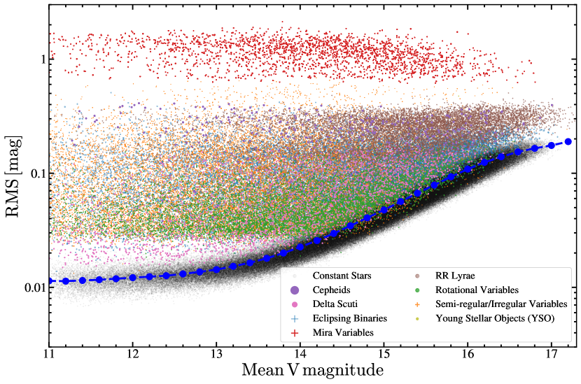
Figure 3: Root-mean-square (RMS) as a function of mean magnitude for the ASAS-SN V-band variable stars with $\rm Prob>0.95$. A sample of $300,000$ constant sources are shown in black. The median RMS of the constant stars is shown in blue for bins of 0.2 mag.

We can estimate the amount of flux blended with the variables using the proximity statistics from refcat2 (Tonry et al., 2018b). Figure 4 shows the distribution of the radius at which the cumulative Gaia $G$-band flux in the aperture exceeds the flux of the variable source (r1). A value of 99$\aas@@fstack{\prime\prime}$9 is assigned when the star is so isolated that the cumulative flux never exceeds the required threshold within the 36$\aas@@fstack{\prime\prime}$0 search radius employed by Tonry et al. (2018b). A large fraction (${\sim}72\%$) of the V-band variables met this criterion. Another ${\sim}11\%$ of the variables had r1$>30"$, and are effectively isolated. Thus, in the context of blending, most (${\sim}83\%$) of the variables can be considered to be relatively isolated. However, a peak corresponding to heavily blended sources is seen at ${\sim}3$$\aas@@fstack{\prime\prime}$0 in Figure 4. Only ${\sim}4\%$ and ${\sim}6\%$ of the variables exceed their flux within an aperture corresponding to the ASAS-SN pixel scale (${\sim}8$$\aas@@fstack{\prime\prime}$0) and FWHM (${\sim}16$$\aas@@fstack{\prime\prime}$0) respectively. The main effect of blending is to reduce the apparent variability amplitude.

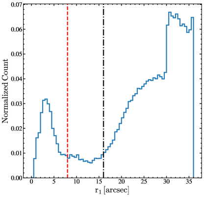
Figure 4: Distribution of the radius at which the cumulative Gaia $G$ flux in the aperture exceeds the flux of the variable source ($\rm r1$ from Tonry et al. (2018b)) for the ASAS-SN V-band variable stars. The ASAS-SN pixel scale (${\sim}8$$\aas@@fstack{\prime\prime}$0) and FWHM (${\sim}16$$\aas@@fstack{\prime\prime}$0) are shown as red dashed and black dot-dashed lines respectively.

Table 1: Variables by type

VSX Type	Description	Known	New	New/Known
CWA	W Virginis type variables with $P>8$ d	243	108	0.44
CWB	W Virginis type variables with $P<8$ d	182	72	0.40
DCEP	Fundamental mode Classical Cepheids	1466	162	0.11
DCEPS	First overtone Cepheids	529	49	0.09
DSCT	$\delta$ Scuti variables	2203	2227	1.01
EA	Detached Algol-type binaries	21399	19329	0.90
EB	$\beta$ Lyrae-type binaries	17078	6956	0.41
EW	W Ursae Majoris type binaries	56431	15415	0.27
HADS	High amplitude $\delta$ Scuti variables	2541	1626	0.64
M	Mira Variables	4612	1661	0.36
ROT	Rotational variables	15218	17624	1.16
RRAB	RR Lyrae variables (Type ab)	16683	5136	0.31
RRC	First Overtone RR Lyrae variables	4380	1808	0.41
RRD	Double Mode RR Lyrae variables	299	71	0.24
RVA	RV Tauri variables (Subtype A)	44	22	0.50
SR	Semi-regular variables	51270	115088	2.24
L	Irregular variables	6584	21110	3.21
GCAS	$\gamma$ Cassiopeiae variables	146	258	1.77
YSO	Young stellar objects	2173	2353	1.08
GCAS:	Uncertain $\gamma$ Cassiopeiae variables	37	71	1.92
VAR	Generic variables	2668	8193	3.07
Total		206218	219351	1.06

During the process of variability classification, we cross-matched the variables with Gaia DR2 (Gaia Collaboration et al., 2018) using a matching radius of 5$\aas@@fstack{\prime\prime}$0. The sources were assigned distance estimates from the Gaia DR2 probabilistic distance estimates (Bailer-Jones et al., 2018) by cross-matching based on the Gaia DR2 source_id. We also cross-matched these sources to the 2MASS (Skrutskie et al., 2006), AllWISE (Cutri & et al., 2013; Wright et al., 2010) and GALEX (Bianchi et al., 2017) catalogues using a matching radius of 10$\aas@@fstack{\prime\prime}$0. We used TOPCAT (Taylor, 2005) for this process. For each source, we also calculate the total line of sight Galactic reddening $E(B-V)$ from the recalibrated ‘SFD’ dust maps (Schlafly & Finkbeiner, 2011; Schlegel et al., 1998). We calculated the absolute, reddening-free Wesenheit magnitudes (Madore, 1982; Lebzelter et al., 2018)

$$W_{RP}=M_{\rm G_{RP}}-1.3(G_{BP}-G_{RP})\,,$$ (1)

and

$$W_{JK}=M_{\rm K_{s}}-0.686(J-K_{s})\,,$$ (2)

for each source, where the $G_{BP}$ and $G_{RP}$ magnitudes are from Gaia DR2 (Gaia Collaboration et al., 2018) and the $J$ and $K_{s}$ magnitudes are from 2MASS (Skrutskie et al., 2006). The Wesenheit magnitudes are important for refining variable type classifications (see Jayasinghe et al. 2019b).

The near-infrared (NIR) $M_{K_{s}}$ vs. $J-K_{s}$ color-magnitude diagram and the $\rm M_{Ks}$ period–luminosity relationship (PLR) diagram for all the variables with variable type classification probabilities $\rm Prob>0.95$, $A_{V}<2$ mag and Gaia DR2 parallaxes better than $20\%$ are shown in Figure 5. Generic and uncertain variable types are not shown. We have sorted the variables into groups to highlight the different classes of variable sources. Rotational variables in our catalog consist of spotted stars on the main-sequence (MS) as well as evolved stars on the red-giant branch (RGB). Semi-regular variables and Mira variables lie on the asymptotic giant branch (AGB). Several PLR sequences are seen in Figure 5. We studied the PLR sequences for the $\delta$ Scuti variables and contact binaries in Papers VI and VII respectively. The slight deficits of variables at the aliases of a sidereal day (e.g., $P\approx 1$ d, $P\approx 2$ d, $P\approx 30$ d, etc.) are due to the quality checks from Jayasinghe et al. (2019c).

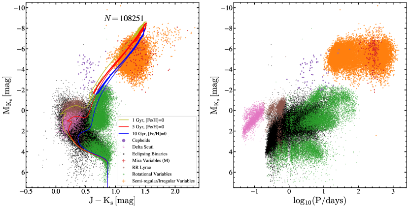
Figure 5: NIR color-magnitude (left) and period-luminosity (right) diagrams for the ASAS-SN V-band variable stars with $\rm Prob>0.95$, $A_{V}<2$ mag and parallaxes better than $20\%$. MIST isochrones (Choi et al., 2016; Dotter, 2016) for single stars with $\rm[Fe/H]=0$ at 1 Gyr, 5 Gyr and 10 Gyr are shown for comparison.

The period-amplitude distribution of the periodic variables is shown in Figure 6. Most variables (${\sim}96\%$) have amplitudes $A<1$ mag. Of the variables with amplitudes $A>1$ mag, ${\sim}59\%$ are Mira and semi-regular variables. Eclipsing binaries (${\sim}22\%$) and RR Lyrae (${\sim}17\%$) are also prominent in this group. Variables with large amplitudes $A>2$ mag are rarer (${\sim}1\%$) and these high amplitude variables are almost exclusively Mira variables.

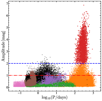
Figure 6: Period-amplitude distributions of the periodic ASAS-SN V-band variables. Reference amplitudes of 1 and 2 mag are shown in red and blue respectively.

3 ASAS-SN Variables in Wide-field spectroscopic surveys

ASAS-SN significantly overlaps with modern major wide-field spectroscopic surveys owing to its all-sky coverage and the magnitude range of the survey. We cross-matched our catalog with the APOGEE DR16 catalog (Holtzman et al., 2015; García Pérez et al., 2016; Ahumada et al., 2019; Jönsson et al., 2020), the RAVE-on catalog (Casey et al., 2017), the LAMOST DR5 v4 catalog (Cui et al., 2012) and the GALAH DR2 catalog (De Silva et al., 2015; Buder et al., 2018) using a matching radius of 5$\aas@@fstack{\prime\prime}$0. LAMOST only reports $\rm T_{eff}$, $\rm\log(g)$, and $\rm[Fe/H]$ for A, F, G and K stars. We identified 39811 (39036) total (unique) matches to the catalogs from the LAMOST (17381), GALAH (3067), RAVE (15050) and APOGEE (4313) spectroscopic surveys.

These spectroscopic surveys differ in their targeting strategy, spectral resolution and data reduction. APOGEE is a NIR survey with a spectral resolving power of $R{\sim}22,500$. LAMOST, RAVE and GALAH are optical surveys with $R{\sim}1,800$, $R{\sim}7,000$ and $R{\sim}28,000$ respectively. The different pipelines that are used in the data reduction process can result in survey specific offsets in the spectroscopic parameters for similar stars. However, efforts have been made to compare the various spectroscopic parameters amongst these surveys, and the parameters are generally similar for most stars (Casey et al., 2017; Buder et al., 2018). The targeting strategies are also different, with APOGEE focusing more on observing red stars than the other surveys. Additionally, variability might impact the derivation of spectroscopic parameters, particularly when sources are in double-lined spectroscopic binaries (eclipsing binaries). Thus, we cannot rely on a single survey to study all the different classes of variable stars.

We illustrate the distribution of the ASAS-SN variable stars with classification probabilities $\rm Prob>0.95$ in $\rm T_{eff}$ and $\rm\log(g)$ (Kiel Diagram) across these surveys in Figure 7. We will only consider sources with $\rm Prob>0.95$ in all of our examinations of spectroscopic properties. We have generally not implemented any cuts on the various flags that are available across these data sets. The LAMOST survey provides the only data set that samples all the major variability classes in our catalog. Most of the cross-matches to APOGEE come from the semi-regular variables and rotational variables. If we implement the data quality cut ASPCAPFLAG=0, ${\sim}65\%$ of the APOGEE sources remain. We note that some fraction of the SR variables with temperatures $\rm T_{eff}<3800$ K in the RAVE data set have values of $\rm\log(g)$ that are inconsistent with being evolved stars on the AGB. If we implement the quality cut QC=0 from Casey et al. (2017), ${\sim}95\%$ of the RAVE sources remain, but this issue with the location of the giants persists. It is also clear that the vast majority of the semi-regular variables in GALAH have incorrect spectroscopic parameters as they populate a non-physical locus in the Kiel diagram. Buder et al. (2018) noted this issue with their pipeline for cool giants with $\rm T_{eff}<4500\,K$. Implementing the data quality cut FLAG_CANNON=0 suggested by Buder et al. (2018), eliminates all but ${\sim}5\%$ of the GALAH sources, which suggests that the GALAH data set is sub-optimal for our purpose of studying variable stars. We find that the data from the LAMOST and RAVE surveys are best suited to characterizing pulsators, eclipsing binaries and rotational variables. APOGEE data are excellent for the characterization of the cooler semi-regular and irregular variables.

The distribution of the variables in $\rm T_{eff}$ and $\rm[Fe/H]$ is shown in Figure 8. We note that the eclipsing binaries in the GALAH sample have metallicities that are largely inconsistent with the eclipsing binaries in the other catalogs. However, only a tiny fraction of this sample passes the quality cut FLAG_CANNON=0. In order to improve the accuracy of our work, we will only consider GALAH sources with FLAG_CANNON=0. We also restrict the RAVE sample of semi-regular variables to those stars with $\rm\log(g)<2$.

The combined distributions of the variables in $\rm T_{eff}$, $\rm\log(g)$, $\rm[Fe/H]$ and $\rm\log_{10}(P/days)$ are shown in Figure 9. The median and standard deviation of the spectroscopic parameters for variable types with sample sizes $N>10$ are also summarized in Table 2. On average, eclipsing binaries have sub-solar metallicities ($\rm[Fe/H]{\sim}-0.2$). Cepheid variables have metallicities consistent with Solar metallicity. $\delta$ Scuti variables and rotational variables have metallicites that are slightly sub-Solar ($\rm[Fe/H]{\sim}-0.1$). Semi-regular variables are strongly peaked at $\rm[Fe/H]{\sim}-0.5$, with very few having Solar or super-Solar metallicities. The population II RRAB stars have very low metallicities with $\rm[Fe/H]{\sim}-1$. The average metallicity of the overtone RR Lyrae (RRC) variables in our sample is $\rm[Fe/H]{\sim}-0.3$ and has a large dispersion of $\sigma{\sim}0.8$ dex. Walker & Terndrup (1991) found that, on average, both RRAB and RRC variables in Baade’s window had $\rm[Fe/H]{\sim}-1$. This suggests that some fraction of the sources classified as RRC variables are in fact EW-type eclipsing binaries with higher metallicities ($\rm[Fe/H]{\sim}-0.2$). Without spectroscopic information, there can be non-negligible confusion between these two variable groups during the classification process due to their very similar and symmetrical light curve shapes.

The temperatures and surface gravities of the semi-regular/irregular variables are consistent with these stars being highly evolved AGB stars. Classical pulsators, such as the RR Lyraes, Cepheids and $\delta$ Scuti variables, have temperatures that fall within the instability strip for pulsations. Overtone Cepheids and RR Lyrae are hotter than the fundamental mode pulsators at fixed temperature. The eclipsing binaries in this sample mostly have surface gravities consistent with main sequence (MS) or slightly evolved stars. Figure 8 shows that the eclipsing binaries span a large range in effective temperature with $\rm 4000\,K<Teff<8000\,K$ (A-K spectral types). On average, $\beta$ Lyrae-type semi-detached binaries (EB) have hotter effective temperatures than both contact binaries and detached eclipsing binaries. The surface gravities of the rotational variables peak near the MS, but the dispersion of $\sigma{\sim}0.8$ dex is large because it is a much more diverse population of sources, including spotted stars on the RGB. We will further investigate the populations of eclipsing binaries and rotational variables in $\S 4$.

Figure 10 shows the correlation between APOGEE and GALAH estimates of $v\sin(i)$ and the ASAS-SN $\rm\log_{10}(P/days)$ for the variables in the spectroscopic sample. As expected for the rotational variables, $v\sin(i)$ decreases with the period. For the 32 semi-regular variables with $v\sin(i)$ measurements from GALAH (APOGEE does not report $v\sin(i)$ for very evolved stars), the median was $v\sin(i){\sim}8\,\rm km/s$. $\delta$ Scuti variables have a broad distribution in $v\sin(i)$, consistent with previous measurements (Solano & Fernley, 1997). Most short period ($\rm P<1$ d) eclipsing binaries have $v\sin(i){\lesssim}20\,\rm km/s$.

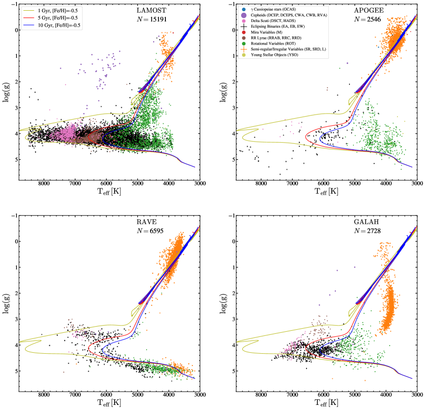
Figure 7: Distributions of the ASAS-SN V-band variables in $\rm\log(g)$ and $\rm T_{eff}$ across the LAMOST, APOGEE, RAVE and GALAH datasets. The points are colored by the variable type. Spectroscopic data quality cuts are not included. MIST isochrones (Choi et al., 2016; Dotter, 2016) for single stars with $\rm[Fe/H]=-0.50$ at 1 Gyr, 5 Gyr and 10 Gyr are shown for comparison.

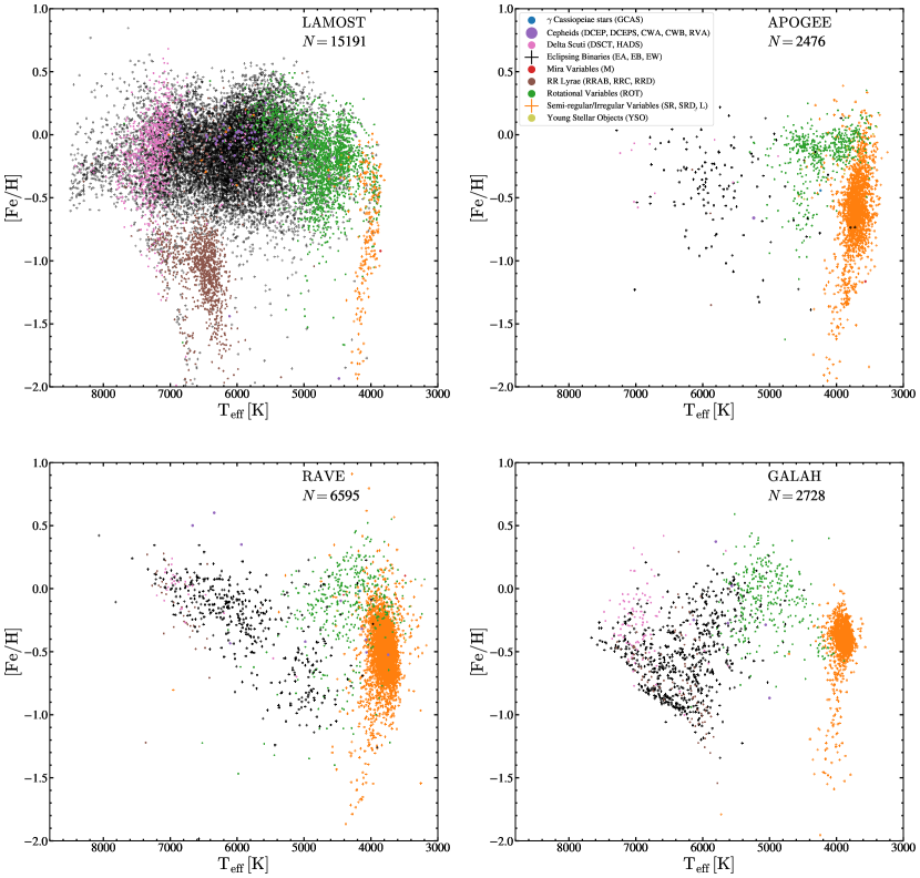
Figure 8: Distributions of the ASAS-SN V-band variables in $\rm T_{eff}$ and $\rm[Fe/H]$ across the LAMOST, APOGEE, RAVE and GALAH datasets. The points are colored by the variable type.

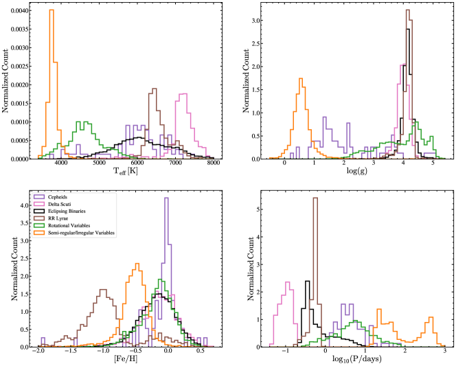
Figure 9: Distributions of the ASAS-SN V-band variables in $\rm T_{eff}$, $\rm\log(g)$, $\rm[Fe/H]$ and $\rm\log_{10}(P/days)$. The histograms are colored by the variable type.

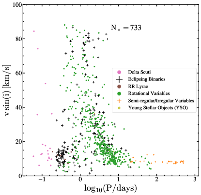
Figure 10: Distributions of the ASAS-SN V-band variables in $v\sin(i)$ vs. $\rm\log_{10}(P/days)$. The points are colored by the variable type.

Table 2: Distribution of $\rm[Fe/H]$, $\rm T_{eff}$ and $\rm\log(g)$ for variable types with at least 10 members with classifications. The variable types are defined in Table 1. The median, and standard deviation for each spectroscopic parameter is shown.

VSX Type	$N$	$\rm T_{eff}$	$\rm\log(g)$	$\rm[Fe/H]$
DCEP	40	6094$\pm$453	1.5$\pm$0.8	$-0.02\pm$0.28
DCEPS	17	6618$\pm$428	2.9$\pm$0.8	0.01$\pm$0.16
DSCT	537	7194$\pm$408	4.0$\pm$0.2	$-0.09\pm$0.27
HADS	267	7256$\pm$538	4.1$\pm$0.2	$-0.24\pm$0.34
EA	3115	6283$\pm$851	4.1$\pm$0.3	$-0.13\pm$0.27
EB	1948	6725$\pm$771	4.1$\pm$0.3	$-0.16\pm$0.27
EW	6388	5905$\pm$656	4.2$\pm$0.2	$-0.17\pm$0.32
SR	7232	3777$\pm$158	0.6$\pm$0.3	$-0.51\pm$0.24
L	371	3773$\pm$212	0.5$\pm$0.4	$-0.47\pm$0.24
ROT	2748	4616$\pm$503	4.1$\pm$0.8	$-0.14\pm$0.28
YSO	27	4188$\pm$497	4.0$\pm$0.9	$-0.21\pm$0.25
RRAB	1086	6477$\pm$297	4.2$\pm$0.2	$-1.01\pm$0.37
RRC	161	6960$\pm$554	4.2$\pm$0.3	$-0.33\pm$0.60
VAR	17	5811$\pm$1262	4.1$\pm$1.8	$-0.90\pm$0.63

4 Discussion

Here we discuss eclipsing binaries, rotational variables and semi-regular variables using both the photometric information from ASAS-SN and other surveys (including Gaia, WISE, 2MASS and GALEX) and spectroscopic information from the cross-matching in $\S 3$ in more detail. In Section $\S 4.1$, we study the temperature and metallicity dependences of the periods of eclipsing binaries. In Section $\S 4.2$, we examine our catalog of rotational variables and particularly the rapidly rotating evolved stars. In Section $\S 4.3$, we discuss the semi-regular variables and their chemical properties using the measurements from APOGEE DR16.

4.1 Eclipsing Binaries

Eclipsing binaries are useful astrophysical tools that can be used to measure the masses and radii of stars across the Hertzsprung-Russell diagram (see Torres et al. 2010, and references therein). We classified ${\sim}136,000$ eclipsing binaries in our catalog into the VSX types: EW (W UMa), EB ($\beta$-Lyrae) and EA (Algol). These classifications were made using a random forest classifier with features derived from light curve characteristics, including Fourier parameters (see Jayasinghe et al. 2019b). EW binaries have light curves with similar primary/secondary eclipse depths whereas EB binaries tend to have eclipses with significantly different depths. Both the EW and EB binaries transition smoothly from the eclipse to the out-of-eclipse state. EA (Algol) binaries are systems where the exact onset and end of the eclipses are easily defined. EA binaries may or may not have a secondary minimum.

Figure 11 shows the distributions of the eclipsing binaries in $\rm\log(g)$, $\rm T_{eff}$, $\rm\log_{10}(P/days)$ and $\rm M_{Ks}$. The surface gravity distributions of the three sub-types are very similar. The biggest differences between the different sub-types are in their effective temperatures. On average, EW type contact binaries are significantly cooler ($\rm T_{eff}{\sim}5900$ K) than both the EB ($\rm T_{eff}{\sim}6700$ K) and the EA systems ($\rm T_{eff}{\sim}6300$ K). EW binaries peak at $\rm\log_{10}(P/days){\sim}-0.5$ and drop sharply at both longer and shorter periods. There are very few EW systems with $\rm\log_{10}(P/days)>0$. EB systems peak at $\rm\log_{10}(P/days){\sim}-0.8$ and span a larger range in period. The detached EA systems peak at $\rm\log_{10}(P/days){\sim}0.4$ and are more evenly distributed in their orbital periods than the EB and EW systems. EW systems are fainter, with a peak at $\rm M_{Ks}{\sim}2.4$ mag, whereas the EB and EA systems peak at a similar $\rm M_{Ks}{\sim}1.6$ mag.

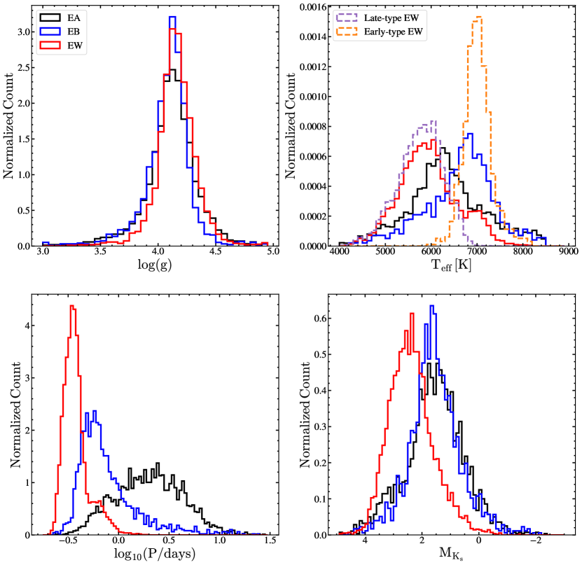
Figure 11: Distributions of the EW (red), EB (blue) and EA (black) binaries in $\rm\log(g)$, $\rm T_{eff}$, $\rm\log_{10}(P/days)$ and $\rm M_{Ks}$. The distributions in $\rm T_{eff}$ for the early (orange) and late-type (purple) EW binaries from Jayasinghe et al. (2020a) are shown as the dashed histograms.

In Paper VII (Jayasinghe et al., 2020a), we analyzed a sample of ${\sim}71,000$ EW systems, and noted a clear dichotomy between the early and late-type EW systems. We found that the period distribution had a clear minimum at $\rm\log(\rm P/d)=-0.30$ which also corresponded to a break in the slope of the period-luminosity relation. The distinction between the populations was even clearer in the space of period and effective temperature, with a gap along the line $\rm T_{eff}=6710K-1760K\,\log(P/0.5\,d)$. The median temperature of the early-type contact binaries ($\rm T_{eff}{\sim}6900$ K) was significantly hotter than the late-type contact binaries ($\rm T_{eff}{\sim}5800$ K). We further noted that the Kraft break (Kraft, 1967) appeared to determine the observed dichotomy of the contact binaries. Early-type systems form due to stellar evolution and the subsequent expansion of a more massive component that is above the Kraft break (${\sim}1.3M_{\odot}$). In contrast, the less massive late-type systems can come into contact due to efficient angular momentum loss during the detached phase (Yıldız, 2014).

Figure 12 shows the different sub-types of eclipsing binaries in the space of $\rm\log(\rm P/d)$ and $\rm T_{eff}$. There is significant overlap in period-temperature space between the EW and EB binaries, with most EB binaries falling above the cut defined in Jayasinghe et al. (2020a) for the early-type EW systems. The overlap between the EW and EB binaries is most significant in the period—temperature space above this cut. The EA binaries are distributed randomly in this space. The distribution of EB binaries peaks at a similar temperature to the early-type EW binaries ($\rm T_{eff}{\sim}6900$ K, see Figure 11), which suggests that the early-type EW are drawn from the population of EB binaries. However, these two populations differ in the ratio between the primary and secondary light curve minima. The degree of thermal equilibrium between the two stars dictates the difference in eclipse depths (Paczyński et al., 2006), and the very similar eclipses seen in EW binaries suggest that these stars are in better thermal contact than the EB binaries that have different eclipse depths.

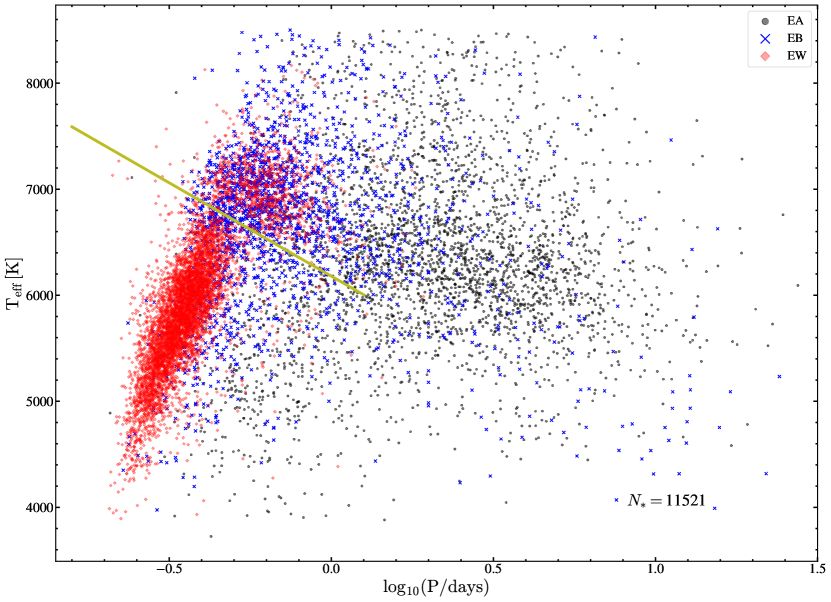
Figure 12: $\rm T_{eff}$ vs. $\rm\log(\rm P/d)$ for EW (red), EB (blue) and EA (black) binaries. The yellow line in $\rm T_{eff}$ and $\rm\log(\rm P/d)$ that separates early and late-type EW binaries is derived in Jayasinghe et al. (2020a).

In our previous work, we hypothesized that the early-type EW systems have a massive component above the Kraft break (${\gtrsim}1.3M_{\odot}$) that is in thermal contact with the secondary. The EB systems are likely to have similar massive components, but the two components in these systems diverge significantly from thermal contact, unlike those in the late-type EW systems. Models of thermal relaxation oscillations (TRO, see, for e.g., Lucy 1976; Flannery 1976; Yakut & Eggleton 2005) predict a population of EB eclipsing binaries with unequal minima that overlap in period and temperature with the EW systems (Webbink, 2003). In the TRO cycle, an eclipsing binary oscillates between the contact and semi-detached states. The semi-detached phase spans a period and temperature range that is comparable to the contact phase, and the two components develop different effective temperatures during the EB stage of the cycle (Webbink, 2003). The overlap between the early-type EW and the EB systems appear to be consistent with the predictions of the TRO models for contact binaries.

The orbital period at which a star overflows its Roche Lobe in a binary consisting of two equal mass stars with a mass ratio of $q=1$ is approximately (Eggleton, 1983)

$${P\over\rm days}\simeq 0.351\left({R_{*}\over R_{\odot}}\right)^{{-3}/2}\left({M_{*}\over M_{\odot}}\right)^{-1/2}.$$ (3)

We used the MIST single star isochrones (Choi et al., 2016; Dotter, 2016) to predict the period-temperature relationship at metallicities of $\rm[Fe/H]=-0.5,\,0$ and $\,0.25$ for a MS population with an age of $10^{8}$ yr. The minimum period for one of the stars to be in Roche contact is weakly dependent on the mass-ratio $q$ (see Eggleton 1983). We illustrate this for a mass ratio of $q=0.1$. The predicted minimum period-temperature relationship depends more strongly on the metallicity— binaries at lower metallicities can have a shorter minimum orbital period at fixed temperature. This relationship is steep for binaries with $\rm T_{eff}\lesssim 7000\,K$ and flattens at higher temperatures. Figure 13 shows the median and $5\%$ to $95\%$ ranges for the periods of eclipsing binaries as a function of temperature. We selected sources with $\log(g)>4$ to restrict the sample to MS binaries. As one would expect, contact EW binaries at fixed $\rm T_{eff}$ have shorter periods than the EB and EA binaries. We see that the lower edge of the EW distribution hugs the Roche limit as expected.

In the MIST model shown in Figure 13, we see that the low metallicity binaries can be more compact before reaching the Roche limit. In Figure 14, we divide each class of eclipsing binaries into metallicity bins of $\rm[Fe/H]<-0.5$, $\rm-0.5<[Fe/H]<0$ and $\rm[Fe/H]>0$, and show the period ranges as a function of temperature for each bin. Most (${\sim}63\%$) eclipsing binaries have metallicities in the range $\rm-0.5<[Fe/H]<0$. Similarly, Pawlak et al. (2019) found that the ASAS-SN eclipsing binaries had a median $\rm[Fe/H]$ 0.2 dex lower than the entire APOGEE DR14 sample. In general, we see that the lower metallicity binaries have shorter periods than the binaries that are metal-rich at fixed temperature.

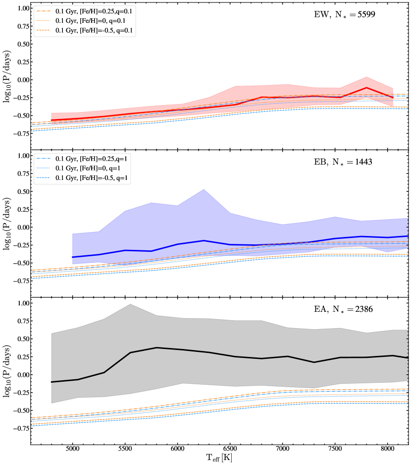
Figure 13: The median $\rm\log(\rm P/d)$ as a function of $\rm T_{eff}$ distributions for EW (top), EB (middle) and EA (bottom) binaries. The shaded regions correspond to the $5\%$ to $95\%$ ranges of the periods. The predicted period-temperature relationships for MS Roche contact binaries with mass ratios $q=1$ (light blue) and $q=0.1$ (orange) is derived using the MIST isochrones (Choi et al., 2016; Dotter, 2016) and are shown for metallicities of $\rm[Fe/H]=-0.50$ (dashed), $\rm[Fe/H]=0$ (dotted) and $\rm[Fe/H]=0.25$ (dot dashed) for a $10^{8}$ yr old stellar population.

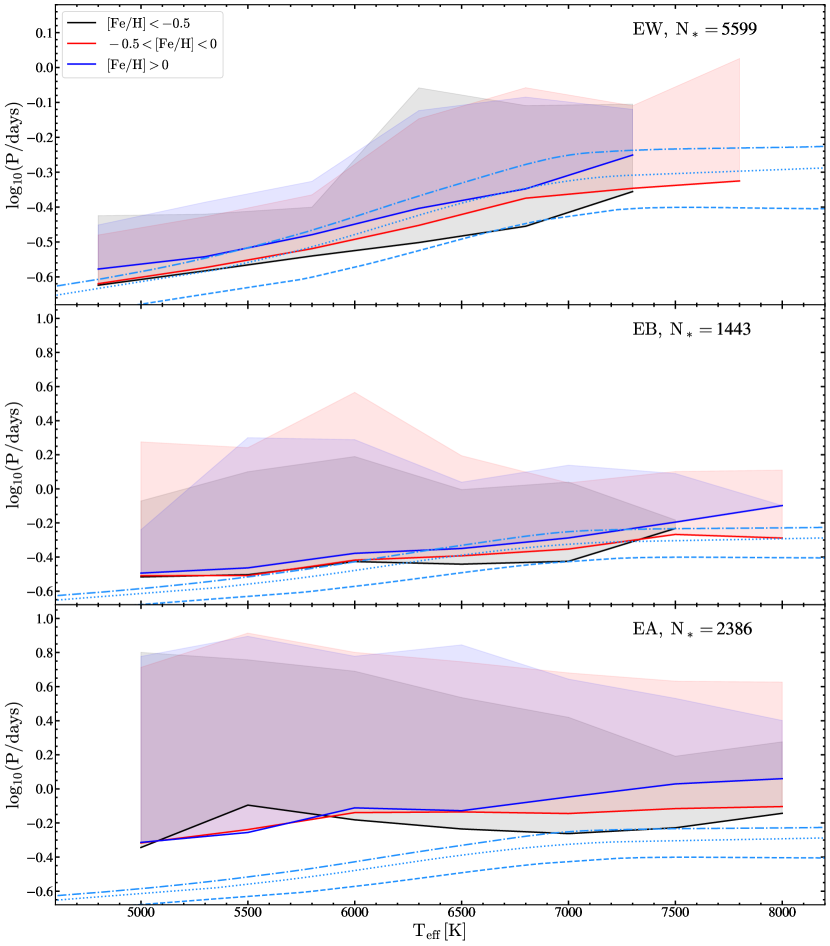
Figure 14: The distribution of the $5^{\rm th}$ percentile in $\rm\log(\rm P/d)$ vs $\rm T_{eff}$ for EW (top), EB (middle) and EA (bottom) binaries in metallicity bins of $\rm[Fe/H]<-0.5$ (black), $\rm-0.5<[Fe/H]<0$ (red) and $\rm[Fe/H]>0$ (blue). The shaded regions correspond to the $5\%$ to $95\%$ ranges of the periods. The predicted period-temperature relationships (light blue) for equal mass MS binaries overflowing their Roche Lobes is derived using the MIST isochrones (Choi et al., 2016; Dotter, 2016) and are shown for metallicities of $\rm[Fe/H]=-0.50$ (dashed), $\rm[Fe/H]=0$ (dotted) and $\rm[Fe/H]=0.25$ (dot dashed) for a $10^{8}$ yr old stellar population.

4.2 Rotational Variables

The ${\sim}33,000$ Rotational (ROT) variables in our V-band catalog are drawn from a variety of rotational variable types, including $\alpha^{2}$ Canum Venaticorum variables (ACV), RS Canum Venaticorum-type (RS) binary systems, BY Draconis-type variables (BY), FK Comae Berenices-type variables (FKCOM), rotating ellipsoidal variables (ELL) and spotted T Tauri stars showing periodic variability (TTS/ROT). Rotational variables are distributed across the Hertzsprung-Russell diagram, but the detectability of a rotational signal largely depends on their evolutionary state. Ceillier et al. (2017) studied ${\sim}17,400$ Kepler red giants and noted that ${\sim}2\%$ of these sources had a detectable rotational signal in their light curves. They also studied ${\sim}600$ red clump stars in their sample and found that ${\sim}15\%$ of these sources had a detectable rotational signal. In contrast, McQuillan et al. (2014) detected periodic rotational signals in the Kepler light curves of ${\sim}25.6\%$ of 133,030 main-sequence stars. Rotational variables found by ASAS-SN must be higher amplitude than the typical examples found by Kepler, favoring spotted stars with large spot covering fractions and/or asymmetric spot coverage (Iwanek et al., 2019).

Figure 15 shows the distributions of the ROT variables in $\rm\log(g)$, $\rm T_{eff}$, $\rm\log_{10}(P/days)$ and $\rm M_{Ks}$. The rotational variables in LAMOST are shown separately, as most spectroscopic cross-matches to the rotational variables come from this catalog. The LAMOST catalog is incomplete for the M-dwarf rotational variables with $\rm\log(g)>4.8$, $\rm T_{eff}<3800$ K. As expected, there are three distinct classes of rotational variables in the $\rm\log(g)$ and $\rm M_{Ks}$ distributions. These correspond to sources on the MS/pre-MS ($\rm\log(g){\sim}4.5$, $\rm M_{Ks}{\sim}4$), sub-giants/giants toward the base of the RGB ($\rm\log(g){\sim}3.5$, $\rm M_{Ks}{\sim}1$) and the red clump ($\rm\log(g){\sim}2.6$, $\rm M_{Ks}{\sim}-1.5$). These three classes of rotational variables have been characterized in previous surveys (see for e.g., McQuillan et al. 2013, 2014; Ceillier et al. 2017). The color-magnitude diagram shown in Figure 5 suggests that sources with $\rm M_{Ks}{\gtrsim}2$ mag are likely to be sub-giants or giants at the base of the RGB. Most of these stars at the base of the RGB will have a sub-giant luminosity class. Red clump (RC) stars have an absolute magnitude of $\rm M_{Ks}=-1.61\pm 0.01$ mag (Hawkins et al., 2017), which is consistent with the peak in the $\rm M_{Ks}$ distribution.

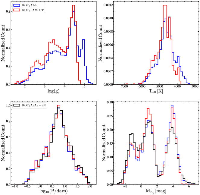
Figure 15: Distributions of the rotational variables for the complete spectroscopic sample (blue) and the LAMOST sample (red) in $\rm\log(g)$, $\rm T_{eff}$, $\rm\log_{10}(P/days)$ and $\rm M_{Ks}$. The $\rm\log_{10}(P/days)$ and $\rm M_{Ks}$ distributions of the rotational variables in the entire ASAS-SN sample are shown in black.

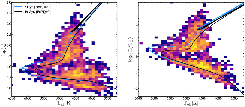
Figure 16: 2-D histograms of the rotation variables in $\rm\log(g)$ (left) and luminosity (right) as a function of $\rm T_{eff}$. The bins are colored by the number density. Solar metallicity MIST isochrones (Choi et al., 2016; Dotter, 2016) for single stars at 5 Gyr and 10 Gyr are shown for comparison.

Figure 16 shows the distribution of rotational variables in $\rm\log(g)$ and luminosity as a function of $\rm T_{eff}$. We use the calibrations from Torres et al. (2010) to derive the radii of the rotational variables using $\rm T_{eff}$, $\rm\log(g)$ and $\rm[Fe/H]$. The Torres et al. (2010) scalings agree with asteroseismic estimates (Yu et al., 2018). The luminosities are then derived using the radius and $\rm T_{eff}$. We find that the rotational variables are largely distributed along the MS and the RGB, with most of the evolved rotational variables located towards the base of the RGB at $\rm\log(g){\sim}3.5$. Rotational variables are also located on the sub-giant branch (SGB). Sources on the red clump are also seen in both of these spaces. There are also many sources above the MS, which are likely spotted stars in binary systems or pre-MS spotted T Tauri stars (TTS/ROT). Of the rotational variables with spectroscopic information, ${\sim}53\%$ (${\sim}47\%$) had $\log(g)>4$ ($\log(g)<4$).

The distribution of the rotational variables in $\rm\log_{10}(P/days)$ or $v_{\rm rot}$ and $\rm\log(g)$ are shown in Figure 17. We estimate the rotational velocities as

$$v_{\rm rot}={2\pi R\over\rm P_{phot}},$$ (4)

where $R$ is estimated using the Torres et al. (2010) calibrations. Regions corresponding to the red clump ($\rm 1.8{\lesssim}\log(g){\lesssim}2.8$) and the SGB/RGB ($\rm 2.9{\lesssim}\log(g){\lesssim}3.9$) are shaded in red and blue, respectively. The stars in the SGB/RGB (RC) region have a median radius and luminosity of $R{\sim}3.4\,R_{\odot}$ ($R{\sim}13.5\,R_{\odot}$) and $\rm L{\sim}5.3\,L_{\odot}$ ($\rm L{\sim}73.3\,L_{\odot}$) respectively. SGB/RGB stars have shorter rotational periods than sources in the red clump, with ${\sim}62\%$ (${\sim}42\%$) of the RGB (RC) rotators having periods $\rm P_{rot}<10$ d. While most of the spectroscopic cross-matches to the rotational variables come from the LAMOST catalog, LAMOST has not released $v\sin(i)$ measurements. However, 78 evolved stars on the SGB/RGB had spectroscopic measurements of $v\sin(i)$ from APOGEE (${\sim}86\%$), or GALAH (${\sim}14\%$) (see Figure 10). The majority (${\sim}81\%$) of these stars were fast rotators with $v\sin(i)>10\rm\,km/s$. We find that ${\sim}80\%$ of the rotational variables on the SGB/RGB have $v_{\rm rot}>10\rm\,km/s$, consistent with the rapid rotators from the sample with spectroscopic $v\sin(i)$. In contrast, ${\sim}98\%$ of the rotational variables on the red clump have $v_{\rm rot}>10\rm\,km/s$.

If we impose a more conservative cut on the red clump sample to minimize contamination from RGB stars by restricting our sample to stars with $\rm 2.3\lesssim\log(g){\lesssim}2.6$, we find that nearly all of these stars have $v_{\rm rot}>10\rm\,km/s$, implying that rapid rotation is more common for red clump stars than for stars on the RGB. To investigate the properties of intrinsically brighter RGB stars, we impose a cut on the SGB/RGB sample to only select RGB stars with $\rm 2.8\lesssim\log(g){\lesssim}3.2$. These stars have a median radius and luminosity of $R{\sim}6.3\,R_{\odot}$ and $\rm L{\sim}17.6\,L_{\odot}$ respectively. We find that ${\sim}84\%$ of these giants have $v_{\rm rot}>10\rm\,km/s$, which is comparable to the broader sample of rotational variables on the SGB/RGB.

Of the rapidly rotating red clump stars, ${\sim}30\%$ are metal-poor with $\rm[Fe/H]<-0.5$, whereas only ${\sim}8\%$ are metal-rich with $\rm[Fe/H]>0$. The multiplicity fraction is anti-correlated with metallicity (see for e.g., Moe et al. 2019), and the prevalence of metal-poor rapid rotators maybe a consequence of higher binary fractions at lower metallicity. Similarly, Tayar et al. (2015) found a large fraction of rapidly-rotating stars on the red clump. This enhancement probably appears because stars are more likely to interact as they expand going up the giant branch, and stop interacting as they descend the giant branch to the red clump. The clump stars then retain the “memory” of the interactions allowed by the expansion. The multiplicity fraction at the red clump is also lower than that of the RGB, and is comparable to the multiplicity fraction at the tip of the RGB (Badenes et al., 2018; Price-Whelan et al., 2020). The reduced multiplicity fraction could be a sign of companion engulfment and spin up during a common envelope phase (Ivanova et al., 2013; Price-Whelan et al., 2020).

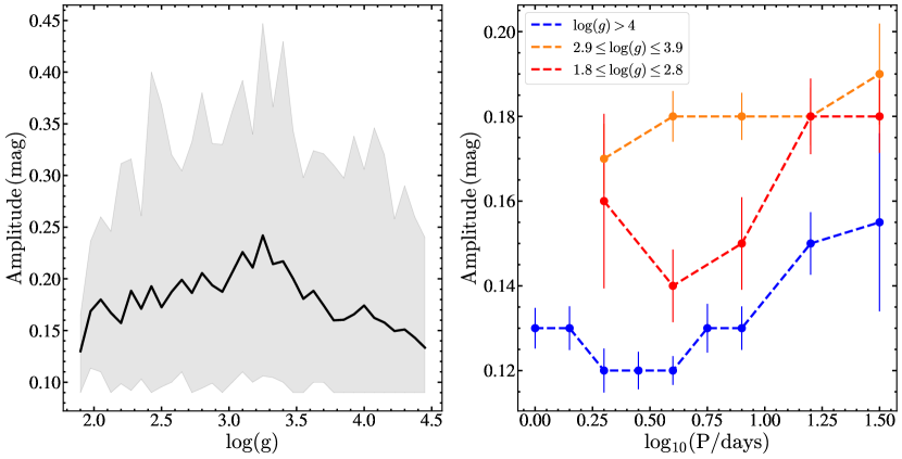
Figure 18: The $V$-band amplitude of the rotational variables in the spectroscopic sample as a function of $\rm\log(g)$ (left) and period (right). The shaded region corresponds to the $5\%$ to $95\%$ range of the amplitudes. The amplitude distributions with period are grouped by $\rm\log(g)$: $\log(g)>4$ (blue), $2.9\leq\log(g)\leq 3.9$ (orange) and $1.8\leq\log(g)\leq 2.8$ (red).

Iwanek et al. (2019) studied 12,660 spotted stars in the Galactic bulge using OGLE data and noted the presence of two distinct groups consisting of rapidly rotating ($\rm P_{rot}<2$ d) stars with low amplitude variability ($A<0.2$ mag in the I-band), and slowly rotating stars with large amplitudes (up to $A<0.8$ mag in the I-band). The sample with large amplitudes mostly consisted of giants. We investigate the $V$-band variability amplitudes of the ASAS-SN rotational variables with spectroscopic information as a function of $\rm\log(g)$ and period in Figure 18. The variability amplitudes of the rotational variables are dependent on their evolutionary state, with the main sequence stars having the lowest amplitudes. The variability amplitudes peak at $\rm\log(g){\sim}3.2$, and drop off again at lower $\rm\log(g)$. At any given period, the evolved rotational variables have larger amplitudes than stars on the MS. This is consistent with the results from Iwanek et al. (2019). The amplitudes of the MS and evolved rotational variables increase at longer periods. Iwanek et al. (2019) noted similar trends in the OGLE sample. Most high amplitude MS rotators in the OGLE sample had long periods, and the spotted giants with long rotational periods showed larger brightness variations, consistent with the trends seen in Figure 18. The large brightness variations in these stars can be attributed to large spot covering fractions and/or longitudinal asymmetries in the coverage of spots (Iwanek et al., 2019).

Of the MS rotational variables with $\log(g)>4$, ${\sim}54\%$ have $v_{\rm rot}>10\rm\,km/s$, compared to ${\sim}83\%$ for evolved stars with $\log(g)<4$. The MS rotators and evolved stars have median periods of $\rm P_{rot}{\sim}3.5$ d and $\rm P_{rot}{\sim}8$ d respectively. A substantial fraction (${\sim}18\%$) of the MS stars have very short periods with $\rm P_{rot}<1$ d (Figure 17). The MS rotators are also more metal-rich ($\rm[Fe/H]{\sim}-0.08$) than the evolved stars ($\rm[Fe/H]{\sim}-0.23$). The median effective temperature for these MS rotators ($\rm T_{eff}{\sim}4460$ K) corresponds to stars with late K spectral types. This is not surprising, as it has been shown that cool MS stars typically have large variability amplitudes and are more likely to show rotational signals than hotter stars (McQuillan et al., 2014), making their detection by ground-based surveys easier. In particular, McQuillan et al. (2014) found that ${\sim}69\%$ of the MS stars with $\rm 4000\leq T_{eff}/K\leq 4500$ K showed periodic rotational variability in their Kepler light curves.

Dixon et al. (2020) identified an empirical relationship between the near-UV (NUV) excess estimated by combining $GALEX$+2MASS data and $v\sin(i)$ for evolved stars in the APOGEE survey. Figure 19 shows the distribution of ${\sim}2,500$ evolved rotational variables with $\rm M_{Ks}<2$ mag (see Figure 5) for which we could calculate the Dixon et al. (2020) NUV excess. Of the sources with GALEX detections, ${\sim}58\%$ have periods $\rm P_{rot}<10$ d. Dixon et al. (2020) derived an empirical rotation-activity relation for giants of

$${\rm NUV\,excess}=(-1.43\pm 0.12)\log(v\sin(i)+(0.647\pm 0.131).$$ (5)

So, giants with $v\sin(i)>10\rm\,km/s$ will have an NUV excess $<-0.78$ mag. We find that ${\sim}87\%$ of the rotating giants have NUV excesses $<-0.78$ mag, which is consistent with our other estimates of the fraction of sources with rapid rotation ($v\sin(i)>10\rm\,km/s$). If we restrict the sources to $\rm M_{Ks}<0$ mag, the fraction of sources with NUV excesses $<-0.78$ mag drops to ${\sim}80\%$.

Dixon et al. (2020) argued that the dependence of the NUV excess on period could be divided into a saturated and a linear regime in activity with a break at $\rm P_{rot}=10$ d. Our sources follow a similar trend, with the median NUV excess decreasing with increasing period beyond $\rm P_{rot}=10$ d (Figure 19). The median NUV excess is roughly flat between $\rm 4<P_{rot}/d<10$, as also found by Dixon et al. (2020). In the super-saturated regime ($\rm P_{rot}\approx 4$ days for typical giants), active giant stars are expected to have decreased activity compared to giants in the saturated regime. We see some evidence for this super-saturated regime in Figure 19.

Figure 20 shows the distribution of all the 248 rotational variables in APOGEE with ASPCAP_FLAG=0 in the $\rm[Mg/Fe]$—$\rm[Fe/H]$ plane as compared to the ${\sim}248,000$ APOGEE DR16 giants with $\log(g)<3.8$ and ASPCAP_FLAG=0. We also show the division from Weinberg et al. (2019) between the “high-$\alpha$” and “low-$\alpha$” sequences. The high-$\alpha$ population is older, kinematically hotter and is located in the thick disk, whereas the low-$\alpha$ population is located in the thin disk (Prochaska et al., 2000; Fuhrmann, 1998; Weinberg et al., 2019). The plateau in the high-$\alpha$ sequence at $\rm[Mg/Fe]{\sim}0.4$ is the average yield of core collapse supernovae and the drop to lower values of $\rm[Mg/Fe]$ is due to later Fe production in type Ia supernovae (Weinberg et al., 2019). The rotational variables are low-$\alpha$ stars strongly clustered towards $\rm[Mg/Fe]{\sim}-0.1$, and $\rm[Fe/H]{\sim}-0.1$. Their distribution in Figure 20 is very different from the typical giant stars or the SR variables and AGB stars we discuss in $\S 4.3.3$. The rotational variables occupy a sparsely populated area in the $\rm[Mg/Fe]$—$\rm[Fe/H]$ plane and this odd clustering of the rotational variables is very likely due to systematics in the ASPCAP abundance pipeline when dealing with rapidly rotating stars. We also highlight 2M05215658+4359220, the candidate giant star-black hole binary identified by Thompson et al. (2019) in Figure 20. 2M05215658+4359220 is a rapidly rotating giant with $v\sin(i)\approx 14.1\pm 0.6\rm\,km/s$ and is a clear outlier in the $\rm[Mg/Fe]$—$\rm[Fe/H]$ plane, even compared to the ROT variables. The ASPCAP pipeline includes the flag ROTATION_WARN to warn of the presence of broadened lines in the APOGEE spectrum, suggesting that the abundances derived for this object could be suspect. The $\rm[C/N]$ abundance of this giant is unusual for a giant with $\rm M_{giant}\approx 3.2\pm 1.0M_{\odot}$ and is more typical of a lower mass giant with $\rm M_{giant}{\sim}1M_{\odot}$ (Thompson et al., 2019). Thompson et al. (2020) cautions against the use of the APOGEE $\rm[C/N]$ abundance in claiming a lower mass for the giant based on the systematic uncertainties in the determination of abundances for rapidly rotating giants. The distribution of the ASAS-SN rotational variables in Figure 20 supports this argument, as their abundances are unusual and suggestive of systematic issues in the ASPCAP pipeline when dealing with rapidly rotating stars. Indeed, if we examine the individual element abundances ($\rm[Fe/Mg]$, $\rm[C/Mg]$, $\rm[Mn/Mg]$ and $\rm[Ni/Mg]$) of the rotational variables, they are almost all peculiar, and those of 2M05215658+4359220 are more peculiar than most.

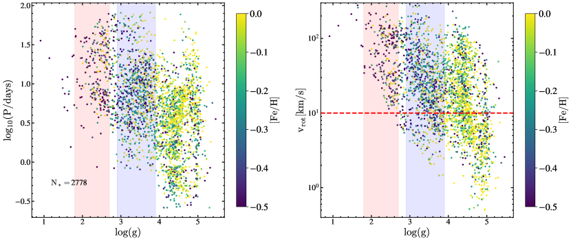
Figure 17: $\rm\log_{10}(\rm P/days)$ (left) and $v_{\rm rot}$ (right) as a function of $\rm\log(g)$ for the rotational variables. The points are colored by metallicity. Regions corresponding to the red clump ($\rm 1.8\lesssim\log(g){\lesssim}2.8$) and the RGB ($\rm 2.9\lesssim\log(g){\lesssim}3.9$) are shaded in red and blue, respectively. The red dashed line corresponds to the division between fast ($v_{\rm rot}>10$ km/s) and slow rotating giants.

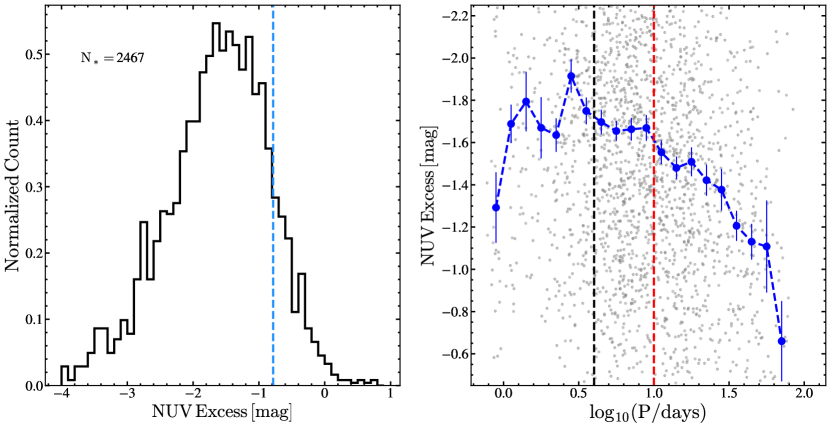
Figure 19: Distributions of the NUV excess (left) and its dependence on period (right) for the rotational variables with $\rm M_{Ks}<2$ mag. The blue dashed line is the expected NUV excess ($-0.78$ mag) for rotating giant stars with $v\sin(i)=10\rm\,km/s$ from Dixon et al. (2020). The red dashed line represents the break in the period-NUV excess relationship at $\rm P_{rot}=10$ days from Dixon et al. (2020). The period at which rotating giants reach super-saturation is shown as a black dashed line at $\rm P_{rot}\approx 4$ days.

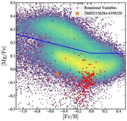
Figure 20: The distribution of all the rotational variables in APOGEE DR16 (red) and a reference sample of giants from APOGEE DR16 (2-d histogram) in the $\rm[Mg/Fe]$ vs. $\rm[Fe/H]$ plane. The blue line shows the division between the low-$\alpha$ and high-$\alpha$ populations from Weinberg et al. (2019). The candidate giant star-black hole binary (2M05215658+4359220) from Thompson et al. (2019) is shown as a orange star.

4.3 Long Period Variables on the Asymptotic Giant Branch

Low and intermediate mass stars end their lives after reaching the asymptotic giant branch (AGB). During the AGB phase, stellar evolution is characterized by hydrogen and helium shell burning on top of a degenerate carbon/oxygen core (see for e.g., Herwig 2005). AGB stars are cool, luminous objects that chemically enrich the interstellar medium through nucleosynthetic processes and strong mass loss (Herwig, 2005; Lebzelter et al., 2018). In particular, the thermally pulsing AGB (TP-AGB) stars are characterized by long-period pulsational variability and heavy mass loss rates (Marigo & Girardi, 2007).

The long-period variables on the TP-AGB are broadly classified into the semi-regular (SR) variables and the Mira variables. Mira variables are luminous AGB stars (Iben & Renzini, 1983) and have large variability amplitudes ($A>2.5$ mag in the V-band is the AAVSO definition). Previous surveys have argued that TP-AGB stars start off as pulsating semi-regular variables with small amplitudes and later evolve into the high amplitude Mira variables as they reach the tip of the AGB (Wood et al., 1999; Marigo & Girardi, 2007; Soszyński et al., 2009). Mira variables follow a period-luminosity relationship (Glass & Evans, 1981; Whitelock et al., 2008), although some Mira variables can undergo changes in their period over time (Percy & Colivas, 1999). Compared to the Mira variables, SR variables are less strictly periodic with irregularities in their light curves and multiple periods that can be used to study the dynamics of stellar interiors (Kiss et al., 1999). Microlensing surveys of the Magellanic clouds have shown that semi-regular variables fall along five distinct period-luminosity sequences (A-E; Wood et al. 1999; Wood 2000). More recent work has shown that the five sequences from Wood et al. (1999) are a result of an overlap of 14 or more period-luminosity sequences (Soszynski et al., 2007; Soszyński et al., 2009; Trabucchi et al., 2017). In the ASAS-SN pipeline, Mira and semi-regular variables are classified on the basis of their periods, colors (optical and near-infrared) and absolute magnitudes (see Jayasinghe et al. 2019b). Semi-regular variables are separated from the Mira variables using their variability amplitudes ($A>2$ mag in the V-band for Miras). We chose a lower limit of $A>2$ mag in amplitude when compared to the AAVSO definition ($A>2.5$ mag) in order to compensate for the effects of blending which can reduce the observed variability amplitudes in ASAS-SN.

We use APOGEE DR16 data (Ahumada et al., 2019) to study the spectroscopic and chemical properties of pulsating AGB stars. The abundances come from the APOGEE Stellar Parameters and Chemical Abundances Pipeline (ASPCAP; Nidever et al. 2015). The various subsets of Mira and SR variables discussed in this section are summarized in Table 3. For comparison with the semi-regular variables, we selected a set of RGB stars (APOGEE/RGB: $\rm T_{eff}\leq 5200$ K, $2\leq\rm\log(g)\leq 3.5$, $N{\sim}160,000$) and likely AGB stars (APOGEE/AGB: $\rm T_{eff}\leq 4000$ K, $\rm\log(g)\leq 1$, $N{\sim}15,000$). The sample of candidate AGB stars is likely contaminated with some lower mass stars on the upper RGB, and does not contain any ASAS-SN SR variables. For detailed studies of the APOGEE DR16 abundance ratios, we required the flag X_FE_FLAG=0, where X= Mg, Al, C, N or O. We calculate the $\rm[X/Mg]$ abundance ratios as $\rm[X/Mg]=[X/H]-[Mg/H]$. Following Weinberg et al. (2019), we chose Mg as the reference element because it is produced almost exclusively by core-collapse supernovae and is thus a simpler tracer of chemical enrichment than Fe.

Table 3: Subsets of Mira and SR variables discussed in $\S$4.3

Group	Description	Criteria	Count	Sections
ALLSPEC/SR	Spectroscopic cross-matches to ASAS-SN SR variables	$\rm Prob>0.95$ and parallaxes better than $50\%$	5,390	$\S$ 4.3.1
ASAS-SN/SR	ASAS-SN SR variables
		$\rm Prob>0.95$ and parallaxes better than $50\%$	96,724	$\S$ 4.3.1
		$\rm Prob>0.95$, $K_{s}$-band photometry available	124,836	$\S$ 4.3.2
ASAS-SN/MIRA	ASAS-SN MIRA variables
		$\rm Prob>0.95$ and parallaxes better than $50\%$	958	$\S$ 4.3.1
		$\rm Prob>0.95$, $K_{s}$-band photometry available	2,737	$\S$ 4.3.2
APOGEE/SR	ASAS-SN SR variables in APOGEE
		$\rm Prob>0.95$ and parallaxes better than $50\%$	991	$\S$ 4.3.1
		$\rm Prob>0.95$	1,615	$\S$ 4.3.2, 4.3.3, 4.3.4, 4.3.5
APOGEE/GIANTS	Giants in APOGEE	$\log(g)<3.8$	238,472	$\S$ 4.3.3
APOGEE/AGB	AGB candidates in APOGEE	$\rm T_{eff}\leq 4000$ K, and $\rm\log(g)\leq 1$	15,050	$\S$ 4.3.3, 4.3.4, 4.3.5
APOGEE/RGB	RGB candidates in APOGEE	$\rm T_{eff}\leq 5200$ K, and $2\leq\rm\log(g)\leq 3.5$	159,042	$\S$ 4.3.3, 4.3.4, 4.3.5

In $\S 4.3.1$, we study the various TP-AGB period-luminosity sequences. We identify an APOGEE temperature—$W_{RP}-W_{JK}$ color index fit to the oxygen-rich AGB stars in $\S 4.3.2$. We examine the $\alpha$ enhancements of the SR variables in $\S 4.3.3$. In $\S 4.3.4$, we study the Aluminum abundances of the semi-regular variables and characterize the pulsation period dependent Al depletion as a result of mass loss and dust production. We look at the Nitrogen abundances of the semi-regular variables in $\S 4.3.5$ and identify a sample of likely intermediate-mass AGB stars undergoing hot-bottom burning.

4.3.1 Period-luminosity sequences

Figure 21 shows the distributions in $\rm\log(g)$, $\rm T_{eff}$, $\rm\log_{10}(P/days)$ and $\rm M_{Ks}$ of the SR variables. The SR variables in APOGEE are shown separately. The spectroscopic parameters confirm the highly evolved nature of these stars, with the SR variables having a median surface gravity of $\rm\log(g){\sim}0.6$, and a median effective temperature of $\rm T_{eff}{\sim}3750$ K. The subset of SR variables in APOGEE DR16 are skewed towards cooler, more evolved SR variables when compared to the SR variables in other surveys. We will only consider the SR variables from APOGEE in the discussions below.

The Gaia DR2 parallaxes of these luminous giants are poor, so we cannot directly assign them to the Wood (2000)’s A-E period-luminosity relations. However, we can use the periods to roughly group them. There are 3 distinct peaks in the period distribution shown in Figure 21 at $\rm\log_{10}(P/days){\sim}1.4,\,1.7,$ and $\,2.7$. SR variables with $1\lesssim\rm\log_{10}(P/days)\lesssim 1.5$ (hereafter group I) fall on the Wood (2000) sequence A and have low variability amplitudes. Due to the overlap between the PLR sequences A and B, SR variables with $1.5\lesssim\rm\log_{10}(P/days)\lesssim 1.9$ (hereafter group II) consist of sources on both sequences A and B. In addition, SR variables on sequence E also have periods in this range, even though they are less luminous than the variables on sequences A and B. The OGLE small amplitude variable red giants (OSARGs; Soszynski et al. 2004) consist of both RGB and AGB stars, and follow a unique set of period-luminosity relations (Soszynski et al., 2007). OSARGs have periods that span group I and have amplitudes as small as ${\sim}3$ mmag (Soszynski et al., 2007; Auge et al., 2020). Note that we are not considering the much lower variability amplitudes of ASAS-SN OSARGs used by Auge et al. (2020) to determine the feasibility of ground-based asteroseismology of luminous giants. There is a paucity of SR variables with periods in the range $1.9\lesssim\rm\log_{10}(P/days)\lesssim 2.3$ (hereafter group III) which spans the PLR sequence C corresponding to the Mira variables. It is thought that the PLR sequence C corresponds to the fundamental mode of pulsation, while sequences A and B correspond to higher order overtone modes (Fraser et al., 2005). SR variables on sequence E are less luminous, and are thought to be on the first ascent giant branch instead of the AGB. SR variables on sequence E have periods typical of contact binaries with a giant component (Wood, 2000) and will be included in groups II and III. SR variables with periods $\rm\log_{10}(P/days)\gtrsim 2.3$ (hereafter group IV) include sources on sequences C and D.

A large fraction of the semi-regular variables with reported periods $\rm\log_{10}(P/days)\gtrsim 2.3$ (sequence D) are examples of semi-regular variables with long secondary periods (LSPs) of $\rm P_{LSP}{\sim}300-1500$ d that are ${\sim}10-15$ times longer than their actual pulsation period (Wood et al., 2004). The origin of the long secondary periods is debated (Wood et al., 2004; Pawlak et al., 2019). These LSPs can complicate our analysis of the pulsational properties of these variables. Thus, we re-derived the periods of the SR variables using the Generalized Lomb-Scargle (GLS, Zechmeister & Kürster 2009; Scargle 1982) periodogram implemented in astrobase (Bhatti et al., 2018). From the 5 best periods in the periodogram, SR variables with LSPs were identified if there was a significantly shorter period $\rm P$ in the range $8\leq\rm P_{LSP}/P\leq 30$ relative to the primary period. For SR variables identified as LSPs, we assign the shorter period as the pulsation period. Of the SR variables with $\rm\log_{10}(P/days)\gtrsim 2.3$, ${\sim}36\%$ were LSPs. This estimate of the LSP fraction at these periods agrees with the estimates (${\sim}25-50\%$) from previous studies (see for e.g., Wood et al. 2004; Soszyński 2007; Nicholls et al. 2009). Of the LSPs, ${\sim}60\%$ had pulsational periods in the range $1.5\lesssim\rm\log_{10}(P/days)\lesssim 1.9$ and the LSP was on average ${\sim}11$ times longer than the actual pulsation period. This agrees with the results from Trabucchi et al. (2017) who found that LSPs had pulsation periods between the PLR sequences B and C’ ($1.5\lesssim\rm\log_{10}(P/days)\lesssim 1.7$). The period distribution of the semi-regular variables after correcting for LSPs is shown in Figure 21. We assign the LSPs into a separate group (group V) for comparison with the other SR variables.

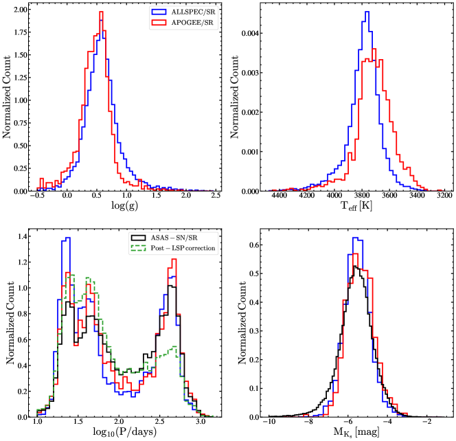
Figure 21: Distributions of the semi-regular variables for the complete spectroscopic sample (blue) and the APOGEE sample (red) in $\rm\log(g)$, $\rm T_{eff}$, $\rm\log_{10}(P/days)$ and $\rm M_{Ks}$. The $\rm\log_{10}(P/days)$ and $\rm M_{Ks}$ distributions of the semi-regular variables in the entire ASAS-SN sample are shown in black. The period distribution of the semi-regular variables after correcting for LSPs is shown in green.

Figure 22 shows the distribution of the SR variables in $\rm M_{Ks}$ (left) and $\rm\log(g)$ with period. SR variables on the PLR sequences A, B and D are prominent, with sources on sequence C largely absent from this sample. The SR variables in these sequences overlap in both the period-luminosity and period-surface gravity spaces. It is difficult to disentangle the PLR sequences given the distance uncertainties — only ${\sim}15\%$ (${\sim}9\%$) of these sources have Gaia DR2 parallaxes better than $20\%$ ($10\%$). The various spectroscopic parameters and chemical abundance ratios from APOGEE DR16 for the five groups (I-V, defined above) are summarized in Table 4.

The median effective temperatures are similar for all the groups, however the median surface gravity for group I is larger than the other groups, suggesting that these sources might be less evolved. Sources in group I might be contaminated with some sources on the upper RGB or are relatively new to the TP-AGB phase. Sources in group III and IV have the largest median $V$-band amplitudes. This is not too surprising as these stars are fundamental-mode pulsators. Sources in group I have the smallest amplitudes, which is consistent with them being overtone pulsators. The metallicities of the sources in groups II, III and IV are largely similar. However, group I has a slightly different chemical profile, with median abundance ratios higher than for the other groups. However, the $\rm[X/Mg]$ abundance ratios are consistent across these groups given the reported dispersions. The biggest difference (${\sim}0.2$ dex) is seen in $\rm[Al/Mg]$, with the median abundance trending from $\rm[Al/Mg]{\sim}-0.1$ for $\rm\log_{10}(P/days)<1.5$ to $\rm[Al/Mg]{\sim}-0.3$ for $\rm\log_{10}(P/days)>1.5$. The LSPs are less evolved than the SR variables in group IV with $\rm\Delta\log(g){\sim}0.1$, and are more similar to the SR variables in group I and II in their properties. This is not surprising given that the pulsation periods of the LSPs are consistent with the periods of SR variables in groups I and II (Trabucchi et al., 2017).

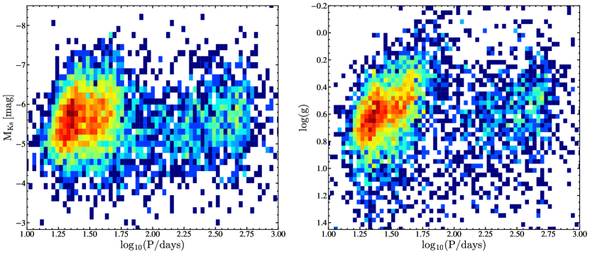
Figure 22: 2-D histograms of $\rm M_{Ks}$ (left) and $\rm\log(g)$ (right) as a function of period for the SR variables in APOGEE DR16 after correcting for LSPs. The bins are colored by the number density.

Table 4: Distribution of the APOGEE DR16 spectroscopic parameters and chemical abundance ratios for the SR variables, binned by period. The SR variables are sorted into period bins as described in the text. The median, and standard deviation for each parameter is shown.

	Group I	Group II	Group III	Group IV	Group V (LSP)
	$1\lesssim\rm\log_{10}(P/days)\lesssim 1.5$	$1.5\lesssim\rm\log_{10}(P/days)\lesssim 1.9$	$1.9\lesssim\rm\log_{10}(P/days)\lesssim 2.3$	$\rm\log_{10}(P/days)\gtrsim 2.3$	$\rm\log_{10}(P/days)\gtrsim 2.3$
$N$	407	475	169	334	300
$\rm Amplitude\,[mag]$	0.11$\pm$0.04	0.20$\pm$0.14	0.29$\pm$0.28	0.30$\pm$0.27	0.16$\pm$0.14
$\rm T_{eff}\,[K]$	3733$\pm$106	3695$\pm$128	3705$\pm$176	3705$\pm$149	3722$\pm$126
$\rm\log(g)$	0.62$\pm$0.20	0.41$\pm$0.22	0.34$\pm$0.41	0.41$\pm$0.31	0.51$\pm$0.24
$\rm[M/H]$	$-0.42\pm$0.23	$-0.63\pm$0.31	$-0.71\pm$0.33	$-0.66\pm$0.29	$-0.57\pm$0.25
$\rm[\alpha/M]$	$0.10\pm$0.09	$0.11\pm$0.10	$0.10\pm$0.11	$0.10\pm$0.11	$0.10\pm$0.10
$\rm[Fe/H]$	$-0.44\pm$0.22	$-0.64\pm$0.29	$-0.71\pm$0.31	$-0.66\pm$0.28	$-0.59\pm$0.24
$\rm[Mg/Fe]$	$0.17\pm$0.11	$0.18\pm$0.11	$0.15\pm$0.13	$0.17\pm$0.12	$0.17\pm$0.11
$\rm[C/Mg]$	$-0.13\pm$0.08	$-0.15\pm$0.15	$-0.16\pm$0.19	$-0.14\pm$0.14	$-0.15\pm$0.11
$\rm[N/Mg]$	$0.05\pm$0.14	$0.00\pm$0.18	$-0.00\pm$0.20	$0.01\pm$0.20	$0.02\pm$0.15
$\rm[O/Mg]$	$-0.03\pm$0.04	$-0.04\pm$0.05	$-0.05\pm$0.06	$-0.05\pm$0.05	$-0.04\pm$0.04
$\rm[Si/Mg]$	$-0.11\pm$0.04	$-0.12\pm$0.05	$-0.12\pm$0.07	$-0.12\pm$0.05	$-0.12\pm$0.04
$\rm[Ca/Mg]$	$-0.08\pm$0.07	$-0.07\pm$0.08	$-0.07\pm$0.11	$-0.08\pm$0.10	$-0.08\pm$0.08
$\rm[Al/Mg]$	$-0.15\pm$0.09	$-0.27\pm$0.16	$-0.35\pm$0.15	$-0.32\pm$0.14	$-0.32\pm$0.14
$\rm[Na/Mg]$	$-0.07\pm$0.14	$-0.09\pm$0.21	$-0.10\pm$0.26	$-0.09\pm$0.23	$-0.10\pm$0.19
$\rm[P/Mg]$	$-0.02\pm$0.13	$-0.06\pm$0.21	$-0.04\pm$0.27	$-0.03\pm$0.25	$-0.04\pm$0.16
$\rm[K/Mg]$	$0.02\pm$0.11	$0.01\pm$0.11	$-0.00\pm$0.12	$0.01\pm$0.11	$0.01\pm$0.10
$\rm[Cr/Mg]$	$-0.17\pm$0.10	$-0.16\pm$0.12	$-0.14\pm$0.17	$-0.15\pm$0.15	$-0.13\pm$0.11
$\rm[V/Mg]$	$-0.06\pm$0.08	$-0.05\pm$0.13	$-0.07\pm$0.13	$-0.06\pm$0.14	$-0.05\pm$0.10
$\rm[Co/Mg]$	$-0.09\pm$0.08	$-0.11\pm$0.09	$-0.10\pm$0.13	$-0.10\pm$0.11	$-0.10\pm$0.10
$\rm[Mn/Mg]$	$-0.06\pm$0.16	$-0.11\pm$0.18	$-0.09\pm$0.19	$-0.09\pm$0.18	$-0.09\pm$0.16
$\rm[Ni/Mg]$	$-0.16\pm$0.08	$-0.17\pm$0.08	$-0.15\pm$0.11	$-0.16\pm$0.10	$-0.17\pm$0.08
$\rm[Ti/Mg]$	$-0.03\pm$0.13	$-0.08\pm$0.14	$-0.11\pm$0.15	$-0.09\pm$0.13	$-0.07\pm$0.13
$\rm[C/N]$	$-0.17\pm$0.14	$-0.17\pm$0.23	$-0.18\pm$0.27	$-0.18\pm$0.24	$-0.18\pm$0.17
$\rm[C/O]$	$-0.10\pm$0.06	$-0.11\pm$0.12	$-0.10\pm$0.17	$-0.10\pm$0.13	$-0.11\pm$0.09
$\rm[N/O]$	$0.07\pm$0.14	$0.05\pm$0.17	$0.06\pm$0.19	$0.07\pm$0.19	$0.07\pm$0.15
$\rm[Al/O]$	$-0.12\pm$0.08	$-0.24\pm$0.14	$-0.28\pm$0.15	$-0.27\pm$0.13	$-0.19\pm$0.12

We compare the periods, amplitudes, bolometric luminosities and radii of the Mira and semi-regular variables with $A_{V}<2$ mag and parallaxes better than $50\%$ in Figure 23. Very few Miras were in the spectroscopic sample. We calculate the bolometric luminosities as

$$\log(L/L_{\odot})=\rm 0.4\big{(}M_{bol,\odot}-M_{Ks}-BC_{K}\big{)},$$ (6)

where $\rm BC_{K}=-6.75\log(\rm T_{eff}/9500)$ is the K-band bolometric correction for stars with $3300\leq\rm T_{eff}/K\leq 5000$ from Buzzoni et al. (2010). The $\rm M_{Ks}$ magnitudes were corrected for extinction using the SFD estimates (Schlafly & Finkbeiner, 2011; Schlegel et al., 1998). The radii are then calculated as

$$\bigg{(}\frac{R}{R_{\odot}}\bigg{)}=\bigg{(}\frac{T}{T_{\odot}}\bigg{)}^{-2}\bigg{(}\frac{L}{L_{\odot}}\bigg{)}^{1/2}.$$ (7)

The bolometric corrections and radii of the SR variables were calculated using the spectroscopic temperatures, whereas we used temperature estimates from Gaia DR2 for the Mira variables. The Mira variables have a median period of $\rm\log_{10}(P/days){\sim}2.5$ ($\rm P{\sim}320$ days). The amplitudes of the Mira variables range from ${\sim}2-6$ mag, whereas most SR variables have amplitudes $<1$ mag. The luminosity distributions of the Mira and SR variables are different, with the Mira variables being more luminous. The median luminosities of the SR variables and Mira variables are $\log(L/L_{\odot}){\sim}3.0$ and $\log(L/L_{\odot}){\sim}3.3$ respectively. Some Mira variables are very luminous, with $\log(L/L_{\odot}){\sim}4$. Paczyński (1970) calculated the maximum luminosity of AGB stars as $\log(L/L_{\odot})=4.74$ based on the core-mass luminosity relationship derived for AGB stars that go through third dredge up. In our sample, all the Mira and SR variables had luminosities below this limit. The median radius of the Mira variables ($R{\sim}132\,R_{\odot}$) is almost twice that of the SR variables ($R{\sim}72\,R_{\odot}$), confirming the more evolved nature of the Mira variables when compared to the SR variables.

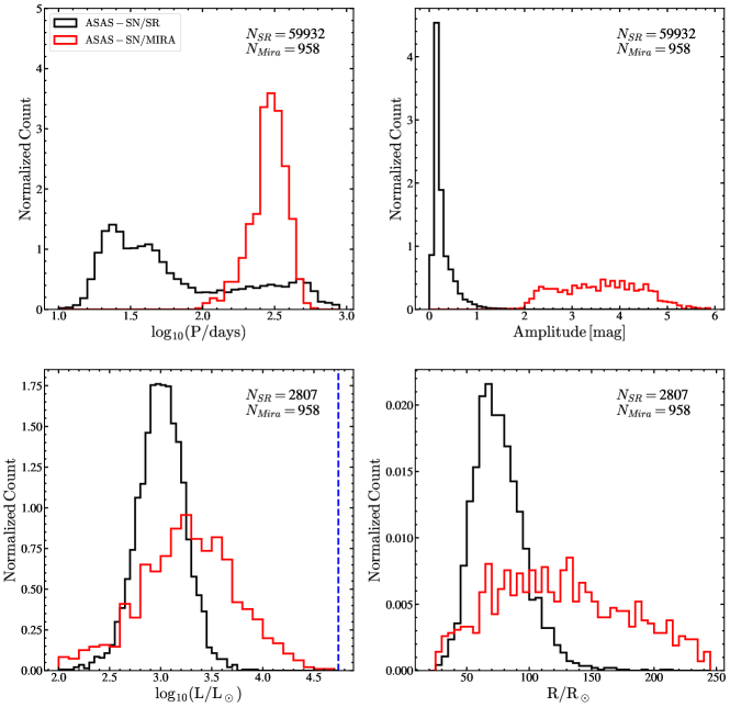
Figure 23: Distributions of the semi-regular variables after correcting for LSPs (black) and Mira variables (red) with $A_{V}<2$ mag and parallaxes better than $50\%$, in $\rm\log_{10}(P/days)$, $V$-band amplitude, $\log(L/L_{\odot})$ and $R/R_{\odot}$. The blue dashed line corresponds to the maximum luminosity of AGB stars ($\log(L/L_{\odot})=4.74$) as calculated by Paczyński (1970).

4.3.2 A multi-band photometric calibration for the temperatures of oxygen-rich AGB stars

Most AGB stars lack spectroscopic information, but well calibrated temperatures are useful for studying these evolved stars. Here, we develop a temperature calibration based on the APOGEE temperatures, and a combination of Gaia and 2MASS photometry. Lebzelter et al. (2018) developed a multi-band approach using the Wesenheit magnitudes, $W_{RP}$ and $W_{JK}$, to distinguish between the various types of AGB stars. The intrinsic spread of red giants in the NIR colors is small, and the Wesenheit magnitudes adequately correct for the interstellar extinction. The visual colors of red giants are more sensitive to their surface temperatures and chemical compositions, resulting in a bigger spread in their optical colors. In their work, Lebzelter et al. (2018) found that the color index $W_{RP}-W_{JK}$ traces the temperature and molecular features in the stellar spectra of AGB stars and that the $W_{RP}-W_{JK}$ index can be used to distinguish between carbon-rich and oxygen-rich AGB stars, with the carbon-rich (oxygen-rich) stars having $W_{RP}-W_{JK}\gtrsim 0.8$ mag ($W_{RP}-W_{JK}\lesssim 0.8$ mag). Arnold et al. (2020) used the $W_{RP}-W_{JK}$ index and the 2MASS $J-Ks$ colors to study long period variables in the KELT survey (Pepper et al., 2007).

We illustrate the distribution of ASAS-SN Mira and semi-regular variables in the ($W_{RP}-W_{JK}$)—($J-Ks$) plane in Figure 24. For reference, we also show the sources from the Catalog of Galactic Carbon Stars (Alksnis et al., 2001). The carbon stars form a sharp, linear locus in this color-color space and have a median $W_{RP}-W_{JK}{\sim}1.5$ mag. In contrast to the carbon rich stars, the oxygen rich sources form a broader and bluer distribution in this plane. The vast majority of the ASAS-SN Mira and semi-regular variables have values of $W_{RP}-W_{JK}$ consistent with oxygen-rich stars. Of the Mira variables and semi-regular variables, ${\sim}97\%$ and ${\sim}95\%$ appear to be oxygen-rich AGB stars, respectively. The carbon-rich semi-regular variables follow the tight carbon-star locus in the $W_{RP}-W_{JK}$—$J-Ks$ plane at $1\,{\rm mag}\lesssim W_{RP}-W_{JK}\lesssim 2\,{\rm mag}$. In general, the carbon-rich semi-regular variables with $W_{RP}-W_{JK}\gtrsim 0.8$ mag have longer median periods ($\rm\log_{10}(P/days){\sim}2.1$) than the oxygen-rich stars ($\rm\log_{10}(P/days){\sim}1.9$). The Mira variables have a distinct distribution in $W_{RP}-W_{JK}$ that skews lower than that of the semi-regular variables.

To investigate the dependence of temperature on the $W_{RP}-W_{JK}$ index, we show the distribution of 1639 semi-regular variables in APOGEE DR16 in the NIR $J-Ks$ color and $\rm T_{eff}$ against the $W_{RP}-W_{JK}$ index in Figure 25. These are essentially all oxygen-rich semi-regular variables because there are few carbon-rich semi-regular variables in the APOGEE data. The temperatures of the oxygen-rich semi-regular variables are remarkably well correlated with the $W_{RP}-W_{JK}$ index for $\rm T_{eff}\lesssim 3800$ K. The semi-regular variables with $\rm T_{eff}\gtrsim 3800$ K have significantly more scatter. We fit a linear relationship of

$$\rm T_{eff}=3548(\pm 2)K+\rm 312(\pm 4)K\,\bigg{(}W_{RP}-W_{JK}\bigg{)}$$ (8)

to the 1191 sources with $\rm T_{eff}<3800\rm\,K$ and $-0.7\,{\rm mag}<W_{RP}-W_{JK}<0.8\,{\rm mag}$. On average, this fit returns temperatures that are within $\pm 0.7\%$ of the APOGEE temperatures. The fit is only done for $-0.7\,{\rm mag}\leq W_{RP}-W_{JK}\leq 0.8\,{\rm mag}$ due to the lack of semi-regular variables with $W_{RP}-W_{JK}<-0.7$ mag.

As a test, we use this relation to estimate the temperatures of the Mira variables shown in Figure 24. The majority of these sources have $W_{RP}-W_{JK}<-0.7$ mag, thus they lie outside the parameter space of the sources used in the fit. Applying equation 8 to these Mira variables, we find the median temperature to be $\rm T_{eff}{\sim}3230$ K (M5 spectral type), with the $1^{\rm st}$ percentile being $\rm T_{eff}{\sim}2800$ K (M8 spectral type) and the $99^{\rm th}$ percentile being $\rm T_{eff}{\sim}3687$ K (M1 spectral type). Mira variables have spectral temperatures that range from M0-M10 (Yao et al., 2017), which is entirely consistent with the extrapolation. Furthermore, the median Gaia DR2 temperature for these Mira variables is $\rm T_{eff}{\sim}3290$ K, which is very similar to the median temperature estimated using equation 8.

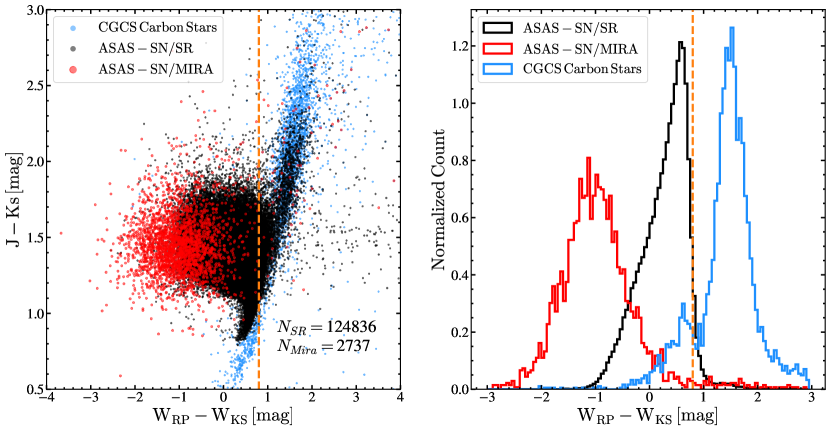
Figure 24: Distributions of the semi-regular variables (black) and Mira variables (red) in $W_{RP}-W_{JK}$ vs. $J-Ks$ (left) and $W_{RP}-W_{JK}$ (right). The sources from the Catalog of Galactic Carbon Stars (Alksnis et al., 2001) (light blue) are also shown for reference. The orange dashed line corresponds to the $W_{RP}-W_{JK}$ index used to separate oxygen-rich ($W_{RP}-W_{JK}\lesssim 0.8$ mag) and carbon-rich ($W_{RP}-W_{JK}\gtrsim 0.8$ mag) AGB stars.

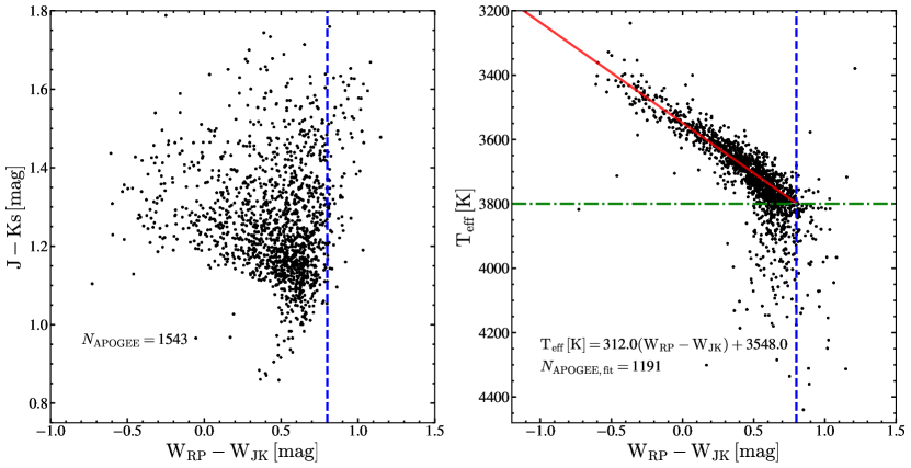
Figure 25: Distributions of the semi-regular variables in APOGEE DR16 in $W_{RP}-W_{JK}$ vs. $J-Ks$ (left) and $W_{RP}-W_{JK}$ vs. $\rm T_{eff}$ (right). The blue dashed line corresponds to the $W_{RP}-W_{JK}$ index ($0.8$ mag) used to separate oxygen-rich and carbon-rich AGB stars. The red line shows the linear fit to the sources with $\rm T_{eff}<3800$ K and $W_{RP}-W_{JK}<0.8$. The green dashed line corresponds to the temperature cutoff of $\rm T_{eff}=3800$ K used in the fit.

4.3.3 $\alpha$-enhancements on the TP-AGB

During the TP-AGB, numerous nuclides are produced during H and He burning. The surfaces of AGB stars are chemically enriched primarily through the third dredge up (TDU) events that follow a thermal pulse. AGB nucleosynthesis depends on the efficiency of the TDU events, the minimum core mass at which TDU begins, the size of the convective envelope, and the mass of the He intershell (Karakas et al., 2002). The efficiency of TDU increases with increasing stellar mass and decreasing metallicity (Karakas et al., 2002). In particular, the surface abundances of CNO elements are enhanced by an order of magnitude or more through successive TDU episodes (Iwamoto et al., 2004). The surfaces of AGB stars are also enriched in heavy elements that are produced by the s-process (e.g., Zr, Sr, Ba, etc., Smith & Lambert 1986, 1988). Hot-bottom burning (HBB) in the more massive AGB stars can also further enhance the surface N abundances (Scalo et al., 1975; McSaveney et al., 2007). Thus, the surface abundances of intermediate-mass AGB stars are dependent on both the TDU and HBB processes.

We show the distribution of the semi-regular variables in the $\rm[Mg/Fe]$—$\rm[Fe/H]$ plane as compared to the distribution of a reference sample of ${\sim}238,000$ giants in APOGEE DR16 with $\log(g)<3.8$ in Figure 26. In the reference sample, ${\sim}27\%$ of the sources belong in the high-$\alpha$ sequence. The bimodality in $\rm[Mg/Fe]$ at sub-solar $\rm[Fe/H]$ is clearly seen for the semi-regular variables as well, but ${\sim}38\%$ of the semi-regular variables lie in the high-$\alpha$ sequence, which is an enhancement of $+41\%$ compared to the overall APOGEE sample.

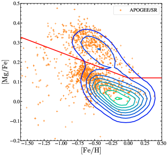
Figure 26: The distribution of the semi-regular variables in the APOGEE DR16 $\rm[Mg/Fe]$ vs. $\rm[Fe/H]$ plane. The contours show the distribution of a reference sample of APOGEE giants. The red line shows the division between the low-$\alpha$ and high-$\alpha$ populations from Weinberg et al. (2019).

We also illustrate the distributions of various surface abundances of the semi-regular variables, APOGEE/RGB stars and APOGEE/AGB stars in Figure 27. The semi-regular variables and the APOGEE/AGB stars are significantly metal-poor. Semi-regular variables with $\rm[Fe/H]>0$ or $\rm[Mg/H]>0$ are rare (${\sim}3\%$ and ${\sim}7\%$). The APOGEE/AGB stars populate the super-solar abundance bins significantly more than the semi-regular variables, but this maybe due to the contamination from metal-rich upper RGB stars. The distributions of $\rm[Na/Mg]$, $\rm[P/Mg]$, and $\rm[Mn/Mg]$ for the three samples are mostly similar. The semi-regular variables and the APOGEE/AGB stars have lower $\rm[C/Mg]$, $\rm[N/Mg]$ and $\rm[O/Mg]$ abundance ratios than the APOGEE/RGB stars. The biggest deviation from the APOGEE/RGB stars is in the distribution of $\rm[Al/Mg]$, with the semi-regular variables peaking ${\sim}-0.3$ dex below the peak of the APOGEE/RGB stars. There are virtually no APOGEE/RGB stars with $\rm[Al/Mg]<-0.25$. There are more semi-regular variables than APOGEE/AGB stars in these lower metallicity bins, perhaps suggesting a pulsational dependence to the $\rm[Al/Mg]$ abundance ratio. We will further investigate this phenomenon in $\S 4.3.4$. The semi-regular variables and APOGEE/AGB stars also show substantial shifts relative to the APOGEE/RGB stars in the $\rm[Si/Mg]$ ($\Delta{\sim}-0.1$ dex), $\rm[Ni/Mg]$ ($\Delta{\sim}-0.1$ dex) and $\rm[Co/Mg]$ ($\Delta{\sim}-0.1$ dex) abundance ratios.

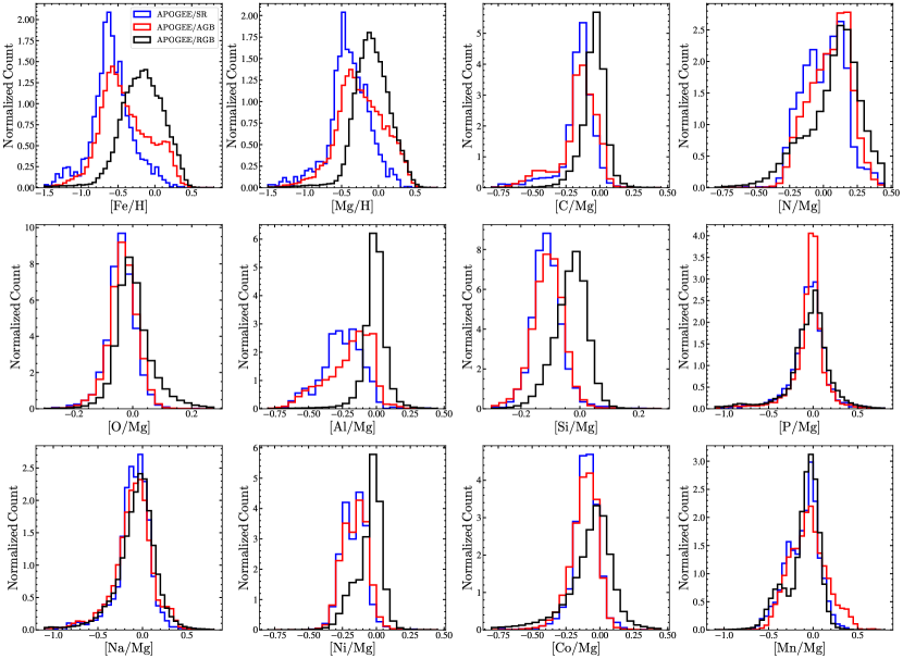
Figure 27: $\rm[Fe/H]$, $\rm[Mg/H]$ and $\rm[X/Mg]$ abundance ratios, where $X=$ C, N, O, Al, Si, P, Na, Ni, Co, and Mn, for the semi-regular variables (blue), APOGEE/AGB stars (red) and APOGEE/RGB stars (black).

While the morphology of the SR distribution in Figure 26 is similar to the APOGEE giants, the actual metallicity and abundance distributions are shifted, as shown in Figure 27 and 28. SR variables tend to be more metal-poor (peak $\rm[Fe/H]{\sim}-0.6$ instead of $\rm[Fe/H]{\sim}-0.2$) and $\alpha$-rich (median $\rm[Mg/Fe]{\sim}0.16$ instead of $\rm[Mg/Fe]{\sim}0.07$). The low-$\alpha$ SR variables peak at $\rm[Mg/Fe]{\sim}+0.12$, compared to $\rm[Mg/Fe]{\sim}+0.03$ for the low-$\alpha$ APOGEE/GIANTS. We illustrate the shifts in the distribution of the $\rm[\alpha/M]$, $\rm[Mg/Fe]$, $\rm[O/Fe]$ and $\rm[Si/Fe]$ abundance ratios in Figure 28. We see significant shifts for both the low-$\alpha$ and high-$\alpha$ stars in all but the $\rm[Si/Fe]$ abundance ratio.

To distinguish between the contribution of (i) the initial abundances at star formation and (ii) dredge-up effects, to the $\rm[\alpha/M]$, $\rm[Mg/Fe]$, $\rm[O/Fe]$ and $\rm[Si/Fe]$ abundance ratios (Figure 28), we re-calculate the peak shifts by limiting the sample of SR variables and APOGEE giants to $\rm-1\leq[Fe/H]\leq-0.25$. In this metallicity-limited sample of SR variables and APOGEE giants, we see that the magnitude of the abundance shifts are smaller, as summarized in Table 5. For example, the peak shift of the low-$\alpha$ SR variables in $\rm[Mg/Fe]$ is now ${\sim}+0.04$, compared to ${\sim}+0.09$ for the full sample. Furthermore, the low-$\alpha$ SR variables appear to have significantly lower median $\rm[Si/Fe]$ abundance ratios than the APOGEE giants. This is suggestive of Si depletion through dust-formation in the winds of these AGB stars (Massalkhi et al., 2018).

These enhancements are suggestive of surface Mg enhancement during TDU episodes. During the AGB, isotopes of Mg are primarily created during thermal pulses through neutron capture processes, and the Ne-Mg reactions (Cristallo et al., 2011). Models of AGB stars have shown that the surface abundance of Mg is enhanced at low metallicities (Cristallo et al., 2011; Cristallo et al., 2015). For example, taking a model of a $1.5\rm M_{\odot}$ AGB star, the final surface $\rm[Mg/Fe]$ abundance ratio is 0.01 at $Z=6\times 10^{-3}$, and 0.43 at $Z=1\times 10^{-3}$ (Cristallo et al., 2011). The efficiency of dredge up also increases with decreasing metallicity (Karakas et al., 2002; Marigo & Girardi, 2007). Considering these theoretical expectations, it is not surprising to see Mg enhancements in the atmospheres of these metal-poor pulsating AGB stars.

In summary, we find that the metallicities and abundance ratios of the SR variables are distinct from the RGB stars. There are more $\alpha$-rich SR variables than $\alpha$-rich RGB stars. The semi-regular variables are more metal-poor with a metallicity peak at $\rm[Fe/H]{\sim}-0.6$. Even after considering the initial abundances at star formation, we find some evidence of $\alpha$/Mg enrichment in the atmospheres of the SR variables, which is likely the result of the third dredge up during the AGB.

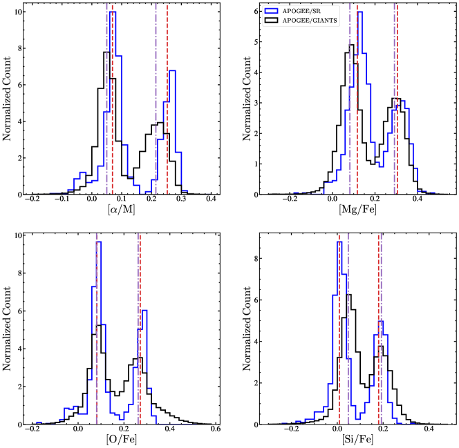
Figure 28: The distribution of the SR variables (blue) and giant stars from APOGEE DR16 in $\rm[\alpha/M]$, $\rm[Mg/Fe]$, $\rm[O/Fe]$ and $\rm[Si/Fe]$. The median abundance ratios of the high-$\alpha$ and low-$\alpha$ SR variables (APOGEE giants) are shown as red (purple) dashed (dot-dashed) lines.

Table 5: The shifts in the median abundance ratios of various $\alpha$ elements between the SR variables and APOGEE/GIANTS. The median abundance error is ${\sim}0.01$ dex.

Abundance	low-$\alpha$ shift	high-$\alpha$ shift	low-$\alpha$ shift	high-$\alpha$ shift
	All	All	Metallicity-limited	Metallicity-limited
$\rm[\alpha/M]$	+0.06	+0.06	+0.02	+0.04
$\rm[Mg/Fe]$	+0.09	+0.04	+0.04	+0.01
$\rm[O/Fe]$	+0.08	+0.05	+0.0	+0.01
$\rm[Si/Fe]$	+0.01	+0.01	-0.04	-0.01

4.3.4 Surface Aluminium depletion on the TP-AGB

Al is a light, odd $Z$ element that is almost entirely produced due to core-collapse supernovae (see for e.g., Weinberg et al. 2019; Griffith et al. 2019). The oxygen-rich atmospheres of most AGB stars are conducive to the formation of dust seeds close to the stellar surface, including $\rm Al_{2}O_{3}$, $\rm SiO_{2}$ and $\rm TiO_{2}$ (Gail et al., 2013; Decin et al., 2017). The presence of alumina ($\rm Al_{2}O_{3}$) dust around oxygen-rich AGB stars is well known (Onaka et al., 1989). Banerjee et al. (2012) reported the near-IR detection of several AlO bands in the wavelength range $1.0-1.35\mu\rm m$ and rotational transitions of this molecule have also been reported (De Beck et al., 2017; Decin et al., 2017). It is thought that AlO is efficiently depleted from the gas around oxygen-rich AGB stars to form alumina dust seeds (De Beck et al., 2017). AGB stars lose mass through a slow wind (${\sim}10\,\rm km/s$) driven by radiation pressure on dust grains (Iben & Renzini, 1983; Khouri et al., 2015). Understanding the formation of dust seeds like alumina and silicate is a crucial consideration when studying mass loss in AGB stars.

In $\S 4.3.3$, we noted that the semi-regular variables and the sample of APOGEE/AGB stars in APOGEE DR16 had lower $\rm[Al/Mg]$ abundance ratios than the APOGEE/RGB stars. The median $\rm[Al/Mg]$ abundance ratios for the semi-regular variables, APOGEE/AGB stars and APOGEE/RGB stars are $-0.25$, $-0.16$ and $-0.01$ respectively. We investigate the $\rm[Al/Mg]$ and $\rm[Al/C]$ abundance ratios for the semi-regular variables, APOGEE/AGB and APOGEE/RGB stars in Figure 29. In the $\rm[Al/Mg]$—$\rm[Mg/H]$ plane, both the semi-regular variables and APOGEE/AGB stars form two distinct sequences of increasing $\rm[Al/Mg]$ with increasing $\rm[Mg/H]$. In general, the APOGEE/AGB stars have higher $\rm[Al/Mg]$ abundance ratios than the semi-regular variables. The $\rm[Al/Mg]$ abundance ratios of the APOGEE/RGB stars appear to follow a Gaussian distribution centered at $\rm[Al/Mg]=0$. Of the APOGEE/RGB stars, only ${\sim}3\%$ have $\rm[Al/Mg]<-0.2$, whereas ${\sim}61\%$ of the semi-regular variables and ${\sim}42\%$ of the APOGEE/AGB stars have $[\rm Al/Mg]<-0.2$. This suggests that Al is being depleted on the AGB, with the pulsating TP-AGB stars depleting more Al than other AGB stars.

The two Al sequences (hereafter the “high-Al” and “low-Al” sequences) are even more distinct in the $\rm[Al/C]$—$\rm[Mg/H]$ plane (Figure 29). The “high-Al” and “low-Al” populations are centered on $\rm[Al/C]{\sim}0$ and $\rm[Al/C]{\sim}-0.15$. The APOGEE/RGB stars again appear to follow a Gaussian distribution in $\rm[Al/C]$, centered at $\rm[Al/C]{\sim}+0.05$. However, both the semi-regular variables and APOGEE/AGB stars have a bi-modal distribution in $\rm[Al/C]$. The semi-regular variables populate the “low-Al” sequence relatively more than the APOGEE/AGB stars, with ${\sim}40\%$ of the semi-regular variables having $[\rm Al/C]<-0.1$ compared to only ${\sim}23\%$ of the APOGEE/AGB stars. This again hints at a correlation between Al depletion and pulsations in AGB stars.

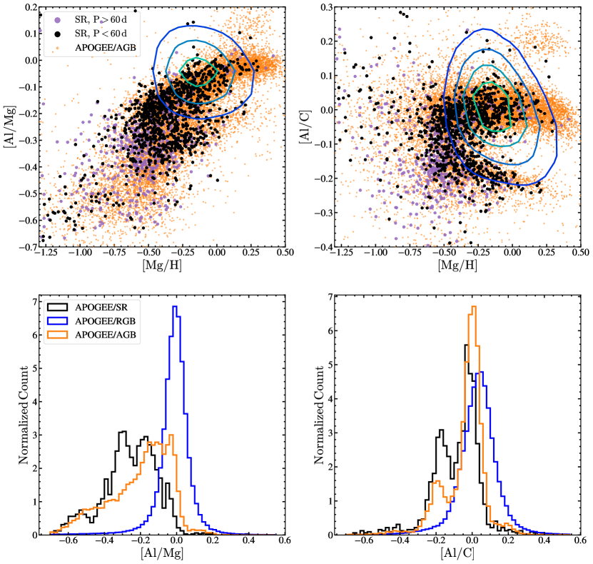
Figure 29: $\rm[Al/Mg]$ (top left) and $\rm[Al/C]$ (top right) vs. $\rm[Mg/H]$ for the semi-regular variables ($\rm P<60$d: black, $\rm P>60$d: purple) and APOGEE AGB stars (orange). The distributions of the APOGEE RGB stars in these planes are shown as contours. The distributions of $\rm[Al/Mg]$ (bottom left) and $\rm[Al/C]$ (bottom right) for the semi-regular variables (black) APOGEE AGB (orange) and RGB (blue) stars are shown as histograms.

We investigate the dependence of $\rm[Al/X]$, where $\rm X=$ Mg, C, Si, O, with the pulsation period in Figure 30. The reference elements C, Si and O, were chosen due to their significant presence in dust grains. Previous studies have established that strong mass loss and increased dust formation first occurs for pulsation periods of $\rm P{\gtrsim}60$ days for Galactic AGB stars (Glass et al., 2009; McDonald et al., 2018). The $\rm[Al/X]$ abundance ratios of the semi-regular variables are strongly correlated with the pulsational period. On average, the $\rm[Al/X]$ abundance ratios decrease with period up until $\rm P{\sim}60$ days and then flatten. The most striking dependence is seen in the distribution of $\rm[Al/O]$ with period. The $\rm[Al/O]$ trend largely plateaus at $\rm[Al/O]{\sim}-0.3$ beyond $P{\sim}60$ days. The fraction of sources with $\rm[Al/O]<-0.22$ varies between the PLR groups (see $\S 4.3.1$), with ${\sim}16\%$ in group I, ${\sim}54\%$ in group II, ${\sim}74\%$ in group III and ${\sim}69\%$ in group IV. The fraction of sources with $\rm[Al/C]<-0.1$ follow a similar trend, with ${\sim}14\%$ in group I, ${\sim}45\%$ in group II, ${\sim}62\%$ in group III and ${\sim}63\%$ in group IV. Of the LSPs, ${\sim}44\%$ and ${\sim}41\%$ had $\rm[Al/O]<-0.22$ and $\rm[Al/C]<-0.1$, respectively. These period trends were far less obvious when we assigned stars their LSPs, which strongly supports the argument that the shorter periods are more physically important.

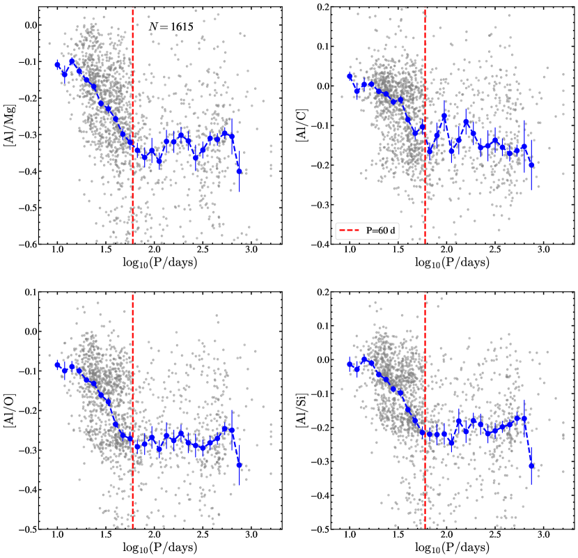
Figure 30: $\rm[Al/Mg]$, $\rm[Al/C]$, $\rm[Al/Si]$ and $\rm[Al/O]$ vs. $\rm\log_{10}(P/days)$ for the semi-regular variables. The binned median abundance ratios are shown in blue. The red dashed line shows the period at which increased dust formation first occurs for Galactic AGB stars ($\rm P{\gtrsim}60$ days). These correlations are far less clear if we use the LSP periods.

Figure 31 shows the dependence of $\rm[Al/X]$, where $\rm X=$ Mg, C, Si, and O, with effective temperature for the semi-regular variables. The high-Al and low-Al sequences that were identified in the $\rm[Al/Mg]$—$\rm[Mg/H]$ and $\rm[Al/C]$—$\rm[Mg/H]$ planes are also apparent in temperature—abundance space. Furthermore, we see evidence of the period dependence on the Al abundance ratios, with short period sources falling into the high-Al sequence. Cuts of $\rm[Al/Mg]=-0.25$, $\rm[Al/C]=-0.1$, $\rm[Al/O]=-0.22$ or $\rm[Al/Si]=-0.13$ roughly separate the high-Al and low-Al sequences. The Al abundance ratios of the high-Al stars decrease with increasing temperature, and is best seen in the trends of the $\rm[Al/O]$ and $\rm[Al/Si]$ abundance ratios with $\rm T_{eff}$. In contrast, the Al abundances of the low-Al stars are not correlated with temperature.

Separating based on their $\rm[Al/C]$ abundance ratio, we find that the high-Al variables have a median period of $\rm\log_{10}(P/days){\sim}1.5\pm 0.4$, whereas the low-Al variables have a median period of $\rm\log_{10}(P/days){\sim}1.8\pm 0.5$. In general, the high-Al variables have periods that fall below the period at which dust formation and mass loss is significant for AGB stars ($\rm\log_{10}(P/days){\sim}1.75$). Most low-Al stars have periods above the canonical threshold ($\rm P{\gtrsim}60$ days) for dust formation in Galactic AGB stars (Figure 30). This suggests that the low-Al sequence could be the result of significant Al depletion through the formation of dust grains containing Al (for example, alumina) in the stellar winds of AGB stars.

The various APOGEE DR16 spectroscopic parameters and chemical abundance ratios for the high-Al and low-Al sequences are summarized in Table 6 for these two groups. The median $V$-band amplitudes of the low-Al stars are more than twice that of the high-Al stars. The high-Al stars have $\rm[\alpha/M]$ abundance ratios that are consistent with being on the low-$\alpha$ sequence, whereas the low-Al stars have $\rm[\alpha/M]$ consistent with being high-$\alpha$ stars. Based on the division in Weinberg et al. (2019), we find that ${\sim}54\%$ of the low-Al stars are high-$\alpha$ stars, whereas only ${\sim}34\%$ of the high-Al variables are on the high-$\alpha$ sequence.

The high-Al stars have enhanced N, Na, P, Cr, Mn, Ni and Ti abundances when compared to the low-Al stars. The low-Al stars tend to have larger Mg abundances ($\rm[Mg/Fe]_{~{}low~{}Al}=0.24\pm 0.12$) and lower metallicities ($\rm[Fe/H]_{~{}low~{}Al}=-0.69\pm 0.28$) when compared to the high-Al stars ($\rm[Mg/Fe]_{~{}high~{}Al}=0.14\pm 0.10$, $\rm[Fe/H]_{~{}high~{}Al}=-0.52\pm 0.25$). The $\rm[Mg/Fe]$ abundance ratios (at star formation) for both the high-$\alpha$ and low-$\alpha$ sequences tend to increase with decreasing metallicity. In addition, models of both low-mass and intermediate-mass AGB stars show that surface $\rm[Mg/Fe]$ is enhanced at low metallicities due to dredge up processes (Cristallo et al., 2011; Cristallo et al., 2015). In $\S 4.3.3$, we showed that the SR variables could be enhanced in Mg through dredge up. Therefore, the larger Mg abundances observed for the low-Al stars can be explained by their birth $\rm[Mg/Fe]$ distribution and possibly with a contribution from dredge up processes in AGB stars.

In summary, an analysis of the $\rm[Al/X]$ abundance ratios of the SR variables show that the Al abundances are correlated with the pulsation period. We identified two distinct sequences amongst the SR variables corresponding to SR variables with high and low Al abundances. The trends of the Al abundances with pulsation period and temperature suggest that the low-Al sequence is likely the result of significant Al depletion through the formation of dust grains containing Al in the stellar winds of AGB stars. The low-Al sequence likely consists of pulsating AGB stars that lose mass through dust-driven winds.

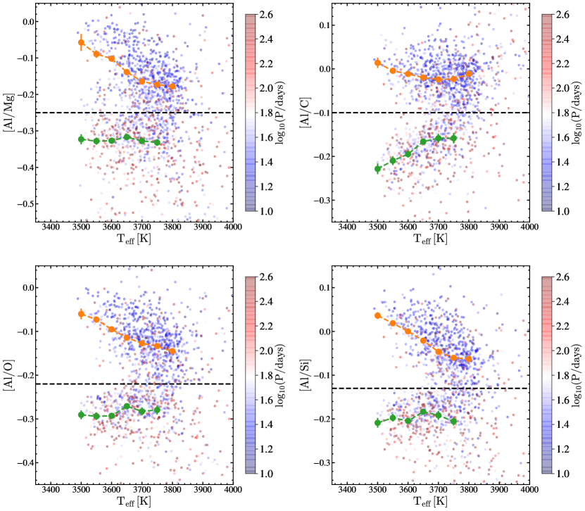
Figure 31: The dependence of $\rm[Al/Mg]$, $\rm[Al/C]$, $\rm[Al/Si]$ and $\rm[Al/O]$ on $\rm T_{eff}$ for the semi-regular variables. The points are colored by $\rm\log_{10}(P/days)$ with the changes in hue at periods near 60 days. The trends in the Al abundance ratios with $\rm T_{eff}$ for the high-Al and low-Al sequences are shown in orange and green respectively. The black dashed line shows the suggested abundance cuts ($\rm[Al/Mg]=-0.25$, $\rm[Al/C]=-0.1$, $\rm[Al/O]=-0.22$ or $\rm[Al/Si]=-0.13$) for separating the high-Al and low-Al sequences.

Table 6: Distribution of the APOGEE DR16 spectroscopic parameters and chemical abundances for the SR variables grouped by their abundances. The SR variables are sorted into these groups based on their $\rm[Al/O]$ and $\rm[N/O]$ abundances. The median, and standard deviation for each parameter is shown.

	High-Al	Low-Al	High-N	Low-N	HBB
	$\rm[Al/O]>-0.22$	$\rm[Al/O]<-0.22$	$\rm 0.02\leq[N/O]\leq 0.3$	$\rm[N/O]<0.02$	$\rm[N/O]>0.30$
$N$	874	812	872	728	86
$\rm\log_{10}(P/days)$	1.5$\pm$0.4	1.8$\pm$0.5	1.6$\pm$0.5	1.6$\pm$0.5	2.0$\pm$0.6
$\rm Amplitude\,[mag]$	0.13$\pm$0.13	0.26$\pm$0.23	0.15$\pm$0.19	0.20$\pm$0.21	0.17$\pm$0.21
$\rm T_{eff}\,[K]$	3730$\pm$126	3683$\pm$139	3727$\pm$126	3677$\pm$120	3822$\pm$194
$\rm\log(g)$	0.54$\pm$0.29	0.42$\pm$0.25	0.46$\pm$0.28	0.55$\pm$0.21	0.07$\pm$0.55
$\rm[M/H]$	-0.50$\pm$0.26	-0.68$\pm$0.29	-0.57$\pm$0.31	-0.63$\pm$0.28	-0.52$\pm$0.31
$\rm[\alpha/M]$	0.08$\pm$0.09	0.22$\pm$0.11	0.07$\pm$0.05	0.25$\pm$0.06	-0.03$\pm$0.07
$\rm[Fe/H]$	-0.52$\pm$0.25	-0.69$\pm$0.28	-0.59$\pm$0.30	-0.64$\pm$0.27	-0.56$\pm$0.30
$\rm[Mg/Fe]$	0.14$\pm$0.10	0.24$\pm$0.12	0.13$\pm$0.07	0.30$\pm$0.08	0.03$\pm$0.09
$\rm[C/Mg]$	$-0.14\pm$0.09	$-0.15\pm$0.16	$-0.14\pm$0.13	$-0.15\pm$0.14	$-0.22\pm$0.18
$\rm[N/Mg]$	$0.08\pm$0.16	$-0.07\pm$0.18	$0.10\pm$0.08	$-0.13\pm$0.09	$0.36\pm$0.19
$\rm[O/Mg]$	$-0.03\pm$0.04	$-0.04\pm$0.05	$-0.04\pm$0.05	$-0.04\pm$0.05	$-0.05\pm$0.05
$\rm[Si/Mg]$	$-0.11\pm$0.05	$-0.12\pm$0.06	$-0.11\pm$0.05	$-0.12\pm$0.05	$-0.08\pm$0.06
$\rm[Ca/Mg]$	$-0.07\pm$0.07	$-0.10\pm$0.10	$-0.06\pm$0.06	$-0.14\pm$0.08	$0.05\pm$0.08
$\rm[Al/Mg]$	$-0.16\pm$0.09	$-0.34\pm$0.11	$-0.20\pm$0.14	$-0.31\pm$0.14	$-0.31\pm$0.14
$\rm[Na/Mg]$	$-0.04\pm$0.15	$-0.14\pm$0.24	$-0.02\pm$0.16	$-0.17\pm$0.20	$0.10\pm$0.17
$\rm[P/Mg]$	$-0.01\pm$0.15	$-0.07\pm$0.25	$0.01\pm$0.17	$-0.11\pm$0.20	$0.18\pm$0.23
$\rm[K/Mg]$	$0.02\pm$0.10	$-0.01\pm$0.11	$0.03\pm$0.10	$-0.02\pm$0.11	$0.09\pm$0.11
$\rm[Cr/Mg]$	$-0.11\pm$0.11	$-0.21\pm$0.15	$-0.08\pm$0.11	$-0.25\pm$0.09	$0.02\pm$0.12
$\rm[V/Mg]$	$-0.04\pm$0.09	$-0.07\pm$0.13	$-0.03\pm$0.12	$-0.09\pm$0.09	$-0.05\pm$0.13
$\rm[Co/Mg]$	$-0.08\pm$0.09	$-0.12\pm$0.11	$-0.06\pm$0.10	$-0.14\pm$0.08	$-0.09\pm$0.12
$\rm[Mn/Mg]$	$-0.04\pm$0.16	$-0.17\pm$0.18	$-0.02\pm$0.14	$-0.24\pm$0.14	$0.02\pm$0.16
$\rm[Ni/Mg]$	$-0.13\pm$0.08	$-0.20\pm$0.09	$-0.11\pm$0.07	$-0.23\pm$0.06	$-0.12\pm$0.10
$\rm[Ti/Mg]$	$-0.06\pm$0.14	$-0.10\pm$0.12	$-0.07\pm$0.16	$-0.09\pm$0.11	$-0.01\pm$0.11
$\rm[C/N]$	$-0.20\pm$0.18	$-0.11\pm$0.24	$-0.23\pm$0.12	$-0.02\pm$0.14	$-0.60\pm$0.32
$\rm[C/O]$	$-0.10\pm$0.07	$-0.11\pm$0.14	$-0.10\pm$0.11	$-0.11\pm$0.11	$-0.17\pm$0.17
$\rm[N/O]$	$0.11\pm$0.15	$-0.03\pm$0.17	$0.13\pm$0.06	$-0.09\pm$0.07	$0.41\pm$0.19
$\rm[Al/O]$	$-0.12\pm$0.07	$-0.29\pm$0.10	$-0.14\pm$0.12	$-0.27\pm$0.12	$-0.27\pm$0.20

4.3.5 Nitrogen Abundances on the TP-AGB

Nitrogen production during the AGB phase is dominated by hot bottom burning (HBB) in intermediate mass stars with $M\gtrsim 3M_{\odot}$ (Scalo et al., 1975; McSaveney et al., 2007). During hot-bottom burning, proton-capture nucelosynthesis occcurs at the base of the outer envelope, favoring the conversion of C to N through the CN cycle (Boothroyd & Sackmann, 1992) where the ${}^{12}\rm C$,${}^{15}\rm N$, ${}^{16}\rm O$ and ${}^{18}\rm O$ isotopes are destroyed to produce ${}^{14}\rm N$ (Lattanzio et al., 1996).This can only happen if the temperature at the bottom of the envelope exceeds ${\sim}50\times 10^{6}$ K (García-Hernández et al., 2013). In these intermediate mass stars, the combination of third dredge-up and hot-bottom burning results in increased N abundances (McSaveney et al., 2007). At the onset of the thermal pulses, hot-bottom burning reduces the ${}^{12}\rm C$ abundance to ${\sim}1/15$ of the MS value and increases the ${}^{14}\rm N$ abundance to ${\sim}5-6$ times the MS value (Lattanzio & Wood, 2004). TDU episodes can continue after HBB ceases to operate, allowing the C abundances to again increase (Frost & Lattanzio, 1996).

We investigate the $\rm[C/Mg]$ and $\rm[C/N]$ abundance ratios for the semi-regular variables, APOGEE AGB and RGB stars in Figure 32. The $\rm[C/Mg]$ abundance ratios for both the semi-regular variables and APOGEE/AGB stars are positively correlated with $\rm[Mg/H]$. The APOGEE/AGB stars and semi-regular variables tend to be carbon-poor when compared to the APOGEE/RGB stars. Only ${\sim}20\%$ of the APOGEE/RGB stars have $\rm[C/Mg]{\lesssim}-0.1$, whereas ${\sim}75\%$ of the semi-regular variables and ${\sim}64\%$ of the APOGEE/AGB stars have $\rm[C/Mg]{\lesssim}-0.1$. The APOGEE/AGB stars form three distinct clusters in the $\rm[C/N]$—$\rm[Mg/H]$ plane at ($-0.4,-0.25$), ($-0.25,0$) and ($0.25,-0.25$). However, the vast majority of the semi-regular variables only populate the two clusters with $\rm[Mg/H]<0$. This is not too surprising as semi-regular variables with $\rm[Mg/H]>0$ are rare in our catalog. The distribution of the APOGEE/RGB stars overlap the metal-rich cluster of APOGEE/AGB stars at ($0.25,-0.25$) that is devoid of semi-regular variables, suggesting that the sample of APOGEE/AGB stars is likely contaminated with stars on the RGB. The distribution of $\rm[C/N]$ is strongly bi-modal for both the semi-regular variables and the APOGEE/AGB stars ($\rm[C/N]{\sim}-0.2$ and $\rm[C/N]{\sim}0$), whereas the APOGEE/RGB stars form a continuous distribution in $\rm[C/N]$, peaking at $\rm[C/N]{\sim}-0.2$. Compared to the APOGEE/RGB stars, there is a small enhancement in the distribution of APOGEE/AGB stars and semi-regular variables with $\rm[C/N]{\lesssim}-0.5$. These are potentially sources with significant N enhancement due to HBB.

In the $\rm[N/Mg]$—$\rm[Mg/H]$ plane (Figure 33), the APOGEE/AGB stars and semi-regular variables form clusters at ($-0.4,0.1$) and ($-0.25,-0.15$). Similarly, in the $\rm[Mg/H]$—$\rm[N/O]$ plane, the APOGEE/AGB stars form three distinct clusters at ($-0.25,-0.1$), ($-0.4,0.15$) and ($0.25,0.15$), with the semi-regular variables populating the two clusters with $\rm[Mg/H]<0$. The distribution of APOGEE/RGB stars in $\rm[N/Mg]$ appears to be bi-modal, with peaks that are similar to those seen for the semi-regular variables and APOGEE/AGB stars. Unlike the APOGEE/RGB stars, the distribution in $\rm[N/O]$ is strongly bi-modal for both the semi-regular variables and APOGEE/AGB stars. We also note the presence of some stars with large $\rm[N/Mg]$ ($\rm[N/Mg]\gtrsim 0.25$) and $\rm[N/O]$ ($\rm[N/O]{\gtrsim}0.3$) abundance ratios. These N-rich sources are candidates for intermediate-mass AGB stars where the surface abundances of N are greatly enhanced due to HBB.

Semi-regular variables and APOGEE/AGB stars with $\rm[N/Mg]{\lesssim}-0.3$ are very rare. Similarly, there is a sharp cutoff in $\rm[N/O]$ for both the semi-regular variables and APOGEE/AGB stars at $\rm[N/O]{\sim}-0.3$. Only ${\sim}0.7\%$ of the semi-regular variables and ${\sim}0.5\%$ of the APOGEE/AGB stars have $\rm[N/O]{\lesssim}-0.3$, whereas ${\sim}4.7\%$ of the APOGEE/RGB stars have $\rm[N/O]{\lesssim}-0.3$. While the N abundances are enhanced and the O abundances are depleted due to the CN cycle, the Mg-Al chain also operates during HBB, destroying the Mg isotopes $\rm{}^{24}Mg$ and $\rm{}^{25}Mg$. In a scenario where HBB operates in an AGB star, the surface abundances of $\rm[N/Mg]$ and $\rm[N/O]$ will increase due to N enrichment and Mg/O depletion. Thus, the observed cutoffs in the $\rm[N/Mg]$ and $\rm[N/O]$ abundance ratios could potentially be related to the nucelosynthetic processes that occur during HBB.

Based on their $\rm[N/O]$ abundance ratios, we group the semi-regular variables into the “high-N” group ($\rm 0.02\leq[N/O]\leq 0.3$), “low-N” group ($\rm[N/O]<0.02$) and intermediate-mass AGB stars that are candidates for HBB ($\rm[N/O]>0.30$). The various APOGEE DR16 spectroscopic parameters and chemical abundance ratios for these groups are summarized in Table 6.

The HBB candidates with $\rm[N/O]>0.30$ are distinct from the high-N and low-N stars. They have significantly lower $\rm\log(g){\sim}0.07$, when compared to the high-N ($\rm\log(g){\sim}0.46$) and low-N ($\rm\log(g){\sim}0.55$) groups. The HBB candidates are generally hotter than the high-N and low-N stars, with a median temperature of $\rm T_{eff}\,{\sim}3822\pm 194$ K. The HBB candidates have a median period of $\rm\log_{10}(P/days){\sim}2$, which is consistent with these stars pulsating in the fundamental mode (Fadeyev, 2017). Much like the high-N stars, the HBB candidates also have low $\rm[\alpha/M]$ abundance ratios ($\rm[\alpha/M]{\sim}-0.04$) consistent with the low-$\alpha$ sequence. The HBB stars have average $\rm[Al/Mg]$ and $\rm[Al/O]$ abundance ratios ($\rm[Al/Mg]{\sim}-0.3$, $\rm[Al/O]{\sim}-0.3$) that are consistent with the low-Al sequence identified in $\S 4.3.4$. Compared to both the high-N and low-N groups, the HBB candidates are poor in Mg and C and they have enhanced N, Ca, Na, P, K, Cr, Mn and Ti abundances compared to both the high-N and low-N groups. The $\rm[C/N]$ abundance ratios of the HBB candidates are significantly different— these HBB candidates have $\rm[C/N]{\simeq}-0.6\pm 0.3$, compared to $\rm[C/N]{\simeq}-0.2\pm 0.1$ for the high-N and $\rm[C/N]{\simeq}0.0\pm 0.1$ for the low-N stars.

The high-N and low-N stars have similar periods, temperatures and $\rm\log(g)$. The slight differences in these measures($\rm\Delta Teff{\sim}50$ K, $\rm\Delta\log(g){\sim}0.1$) might suggest that the high-N stars are somewhat more evolved and hotter than the low-N stars. The high-N stars have $\rm[\alpha/M]$ abundance ratios that are consistent with them being on the low-$\alpha$ sequence, whereas the low-N stars have $\rm[\alpha/M]$ consistent with them being high-$\alpha$ stars. The low-N stars have larger Mg abundances ($\rm\Delta[Mg/Fe]{\sim}0.2$ dex) than the high-N stars. The $\rm[Al/Mg]$ and $\rm[Al/O]$ abundance ratios of the low-N stars are lower than that of the high-N stars and possibly indicate that these stars are undergoing mass loss. The high-N stars have enhanced N, Ca, Na, P, K, Cr, V, Co, Mn, and Ni abundances when compared to the low-N stars.

In summary, we identified a “high-N” group ($\rm 0.02\leq[N/O]\leq 0.3$), and a “low-N” group ($\rm[N/O]<0.02$) amongst the SR variables. The high-N stars differ in their chemical profiles when compared to the low-N stars. We also identified a sample of N-enhanced, likely intermediate-mass AGB stars ($\rm[N/O]>0.30$) going through significant hot-bottom burning (HBB). We also find that the HBB candidates are carbon poor with $\rm[C/N]{\sim}-0.6$.

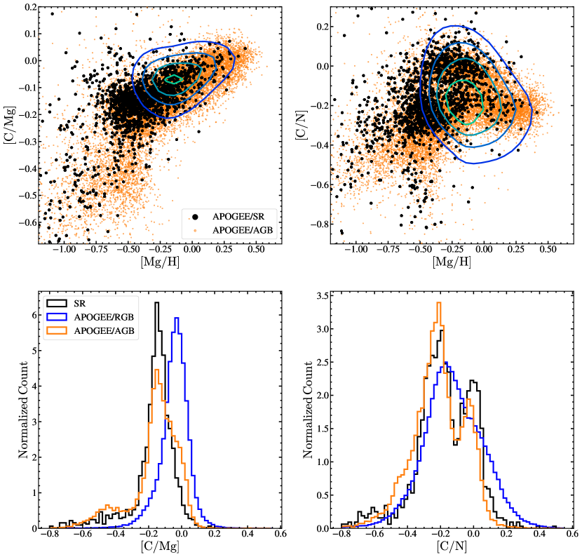
Figure 32: $\rm[C/Mg]$ (top left) and $\rm[C/N]$ (top right) vs. $\rm[Mg/H]$ for the semi-regular variables (black) and APOGEE AGB stars (orange). The distributions of the APOGEE RGB stars in these planes are shown as contours. The distributions of $\rm[C/Mg]$ (bottom left) and $\rm[C/N]$ (bottom right) for the semi-regular variables (black) APOGEE AGB (orange) and RGB (blue) stars are shown as histograms.

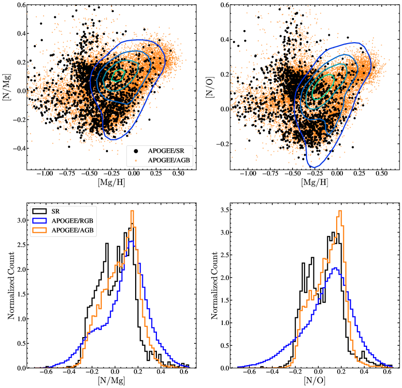
Figure 33: $\rm[N/Mg]$ (top left) and $\rm[N/O]$ (top right) vs. $\rm[Mg/H]$ for the semi-regular variables (black) and APOGEE AGB stars (orange). The distributions of the APOGEE RGB stars in these planes are shown as contours. The distributions of $\rm[N/Mg]$ (bottom left) and $\rm[N/O]$ (bottom right) for the semi-regular variables (black) APOGEE AGB (orange) and RGB (blue) stars are shown as histograms.

5 Conclusions

We systematically searched for variable sources in ASAS-SN with $V<17$ mag in the $V$-band light curves of ${\sim}61.5$ million sources. Through our search which first began in 2018, we identified ${\sim}426,000$ variable sources, of which ${\sim}219,000$ are new discoveries. The V-band light curves of all the ${\sim}61.5$M sources studied in this work are available online at the ASAS-SN Photometry Database (https://asas-sn.osu.edu/photometry). The $V$-band light curves and other information on the variable stars identified in our work are available on the ASAS-SN variable stars database (https://asas-sn.osu.edu/variables). ASAS-SN has significantly improved the census of semi-regular/irregular variables ($+235\%$), $\delta$ Scuti variables ($+81\%$), rotational variables ($+116\%$) and detached eclipsing binaries ($+90\%$) with $V<17$ mag. Most (${\sim}74\%$) of our discoveries were in the Southern hemisphere.

Due to the overlap between ASAS-SN and modern major wide-field spectroscopic surveys, we are able to utilize spectroscopic information to closely study various variable types. We cross-matched our catalog of variables with the APOGEE DR16 catalog, the RAVE-on catalog, the LAMOST DR5 v4 catalog and the GALAH DR2 catalog, and identified ${\sim}39,000$ unique cross-matches. We find that data from the LAMOST and RAVE surveys are best suited to the characterization of pulsators, eclipsing binaries and rotational variables. APOGEE data is excellent for the characterization of the cooler semi-regular and irregular variables. Our main results for eclipsing binaries, rotational variables and semi-regular variables are summarized below.

Eclipsing binaries:

1. EW type contact binaries are significantly cooler ($\rm T_{eff}{\sim}5900$ K) than both the semi-detached EB binaries ($\rm T_{eff}{\sim}6700$ K) and the detached EA systems ($\rm T_{eff}{\sim}6300$ K).

2. There is significant overlap in period—temperature space between the early-type EW and EB binaries. This overlap is consistent with the predictions of the thermal relaxation oscillation (TRO) models for contact binaries, where systems can transition between the semi-detached and contact phases.

3. Most (${\sim}63\%$) eclipsing binaries have metallicities $\rm-0.5<[Fe/H]<0$. This is consistent with recent findings of higher binary fractions at lower metallicity (Badenes et al., 2018; Moe et al., 2019; El-Badry & Rix, 2019).

4. The period—temperature distributions depend on metallicity, with lower metallicity binaries having shorter periods at fixed temperature.

5. Contact binaries have an observed period-temperature relationship that falls below that of the semi-detached and detached binaries at any given temperature and tracks Roche expectations.

Rotational variables:

1. We find rotational variables on the MS/pre-MS ($\rm\log(g){\sim}4.5$, $\rm M_{Ks}{\sim}4$ mag), the base of the red-giant branch ($\rm\log(g){\sim}3.5$, $\rm M_{Ks}{\sim}1$ mag) and the red clump ($\rm\log(g){\sim}2.6$, $\rm M_{Ks}{\sim}-1.5$ mag).

2. ${\sim}81\%$ of the rotating giants with spectroscopic $v\sin(i)$ were rapid rotators with $v\sin(i)>10\rm\,km/s$.

3. ${\sim}80\%$ of the giants have $v_{\rm rot}>10\rm\,km/s$, consistent with the estimate of rapid rotators with spectroscopic $v\sin(i)$.

4. ${\sim}98\%$ of the rotational variables on the red clump have $v_{\rm rot}>10\rm\,km/s$.

5. ${\sim}30\%$ of the rapidly rotating red clump stars are metal-poor with $\rm[Fe/H]<-0.5$, whereas only ${\sim}8\%$ are metal-rich with $\rm[Fe/H]>0$.

6. ${\sim}87\%$ of the rotating giants had NUV excesses from Dixon et al. (2020) consistent with $v\sin(i)>10\rm\,km/s$. This is consistent with our other estimates of the fraction of sources with rapid rotation ($v\sin(i)>10\rm\,km/s$).

7. Evolved rotating giants have larger amplitudes than main-sequence rotational variables at any given period, with the variability amplitudes peaking at $\rm\log(g){\sim}3.2$.

8. The NUV excesses of these rotating giants follow a similar trend with period to the work of Dixon et al. (2020).

9. The rotational variables in APOGEE are low-$\alpha$ stars strongly clustered towards $\rm[Mg/Fe]{\sim}-0.1$, and $\rm[Fe/H]{\sim}-0.1$, distinct from the typical giant stars or the SR variables and AGB stars. These abundances are unusual and suggestive of systematic issues in the ASPCAP pipeline when dealing with rapidly rotating stars.

Semi-regular variables and Miras:

1. Semi-regular variables tend to be lower metallicity ($\rm[Fe/H]{\sim}-0.5$) than most giant stars.

2. Of the semi-regular variables with $\rm\log_{10}(P/days)\gtrsim 2.3$, ${\sim}36\%$ were LSPs. ${\sim}60\%$ of the LSPs had pulsational periods in the range $1.5\lesssim\rm\log_{10}(P/days)\lesssim 1.9$. The LSP was on average ${\sim}11$ times longer than the actual pulsation period.

3. Many semi-regular variables have LSPs, and while it seems clear that the shorter period rather than the LSP is more closely related to the physical properties of the star, we could identify no spectroscopic property ($\rm T_{eff}$, $\rm\log(g)$, abundances etc.) which distinguished SR variables with LSPs from those without.

4. The vast majority of the ASAS-SN Mira (${\sim}97\%$) and semi-regular variables (${\sim}95\%$) are oxygen-rich AGB stars.

5. We fit a temperature—$W_{RP}-W_{JK}$ relation that returns temperatures that are, on average, within $\pm 0.7\%$ of the APOGEE temperatures for the oxygen-rich SR variables with $\rm T_{eff}<3800$ K and $-0.7{\,\rm mag}\leq W_{RP}-W_{JK}\leq 0.8{\,\rm mag}$. We tested an extrapolation of this temperature—$W_{RP}-W_{JK}$ relation to estimate the temperatures of the Mira variables with $W_{RP}-W_{JK}<-0.7$ mag. We find the results of our extrapolation consistent with the expected temperatures of Miras (Yao et al., 2017).

6. The peak shifts in the $\rm[Mg/Fe]$, and $\rm[\alpha/M]$ abundance ratios for the high-$\alpha$ and low-$\alpha$ stars relative to the APOGEE giants indicate possible $\alpha$-enhancements due to the effects of the third dredge up in AGB stars.

7. The $\rm[Al/X]$ abundance ratios of the semi-regular variables are correlated with the pulsation period. These abundance ratios decrease with period and plateau beyond the canonical period of $P{\sim}60$ days where dust formation first occurs.

8. We identified a “high-Al” and a “low-Al” sequence amongst the SR variables. The Al depleted “low-Al” sequence likely corresponds to AGB stars with significant dust production and mass loss. Cuts of $\rm[Al/Mg]=-0.25$, $\rm[Al/C]=-0.1$, $\rm[Al/O]=-0.25$ or $\rm[Al/Si]=-0.13$ roughly separate the high-Al and low-Al sequences.

9. We identified a “high-N” group ($\rm 0.02\leq[N/O]\leq 0.3$), and a “low-N” group ($\rm[N/O]<0.02$) amongst the SR variables. The high-N stars have enhanced Ca, N, Na, P, K, Cr, V, Co, Mn, and Ni abundances when compared to the low-N stars.

10. We identified a sample of likely intermediate-mass AGB stars going through significant hot-bottom burning (HBB) using the cutoff $\rm[N/O]>0.30$. The HBB candidates are poor in Mg and C ($\rm[C/N]{\sim}-0.6$), but have enhanced N, Ca, Na, P, K, Cr, Mn and Ti abundances compared to both the high-N and low-N groups.

This work is a first exploration of the powerful synergy between wide-field photometric and spectroscopic surveys towards deciphering the various properties of variable stars. As the number of stars with spectroscopic measurements increases by orders of magnitude over the coming years, it will be possible to study much larger samples of variable stars in greater detail. While we have not examined it here, larger samples with models of selection effects can be used to examine the detailed fractions of variable types as a function of their spectroscopic properties, similar to the recent studies of the dependence of binary fraction on metallicity (Badenes et al., 2018; Moe et al., 2019; El-Badry & Rix, 2019).

Data Availability

The ASAS-SN photometric data underlying this article are available on the ASAS-SN Photometry Database (https://asas-sn.osu.edu/photometry) and the ASAS-SN variable stars database (https://asas-sn.osu.edu/variables). The external photometric data underlying this article were accessed from sources in the public domain: Gaia (https://www.cosmos.esa.int/gaia), 2MASS (https://old.ipac.caltech.edu/2mass/overview/access.html), AllWISE (http://wise2.ipac.caltech.edu/docs/release/allwise/) and GALEX (https://archive.stsci.edu/missions-and-data/galex-1/). The spectroscopic datasets underlying this article were accessed from sources in the public domain: APOGEE (https://www.sdss.org/dr16/), LAMOST (http://dr5.lamost.org/), GALAH (https://galah-survey.org/publicdata/) and RAVE (https://www.rave-survey.org/).

References

- Ahumada et al. (2019) Ahumada R., et al., 2019, arXiv e-prints, p. arXiv:1912.02905
- Alard (2000) Alard C., 2000, A&AS, 144, 363
- Alard & Lupton (1998) Alard C., Lupton R. H., 1998, ApJ, 503, 325
- Alcock et al. (1997) Alcock C., et al., 1997, ApJ, 486, 697
- Alksnis et al. (2001) Alksnis A., Balklavs A., Dzervitis U., Eglitis I., Paupers O., Pundure I., 2001, Baltic Astronomy, 10, 1
- Arnold et al. (2020) Arnold R. A., et al., 2020, ApJS, 247, 44
- Auge et al. (2020) Auge C., et al., 2020, arXiv e-prints, p. arXiv:2003.05459
- Badenes et al. (2018) Badenes C., et al., 2018, ApJ, 854, 147
- Bailer-Jones et al. (2018) Bailer-Jones C. A. L., Rybizki J., Fouesneau M., Mantelet G., Andrae R., 2018, AJ, 156, 58
- Banerjee et al. (2012) Banerjee D. P. K., Varricatt W. P., Mathew B., Launila O., Ashok N. M., 2012, ApJ, 753, L20
- Beaton et al. (2018) Beaton R. L., et al., 2018, Space Sci. Rev., 214, 113
- Bellm et al. (2019) Bellm E. C., et al., 2019, PASP, 131, 018002
- Bhatti et al. (2018) Bhatti W., Bouma L., Joshua John Price-Whelan A., 2018, Waqasbhatti/Astrobase: Astrobase V0.3.20, doi:10.5281/zenodo.1469822
- Bianchi et al. (2017) Bianchi L., Shiao B., Thilker D., 2017, ApJS, 230, 24
- Blanton et al. (2017) Blanton M. R., et al., 2017, AJ, 154, 28
- Boothroyd & Sackmann (1992) Boothroyd A. I., Sackmann I. J., 1992, ApJ, 393, L21
- Bredall et al. (2020) Bredall J. W., et al., 2020, arXiv e-prints, p. arXiv:2005.14201
- Brown et al. (2013) Brown T. M., et al., 2013, PASP, 125, 1031
- Buder et al. (2018) Buder S., et al., 2018, MNRAS, 478, 4513
- Buzzoni et al. (2010) Buzzoni A., Patelli L., Bellazzini M., Pecci F. F., Oliva E., 2010, MNRAS, 403, 1592
- Casey et al. (2017) Casey A. R., et al., 2017, ApJ, 840, 59
- Ceillier et al. (2017) Ceillier T., et al., 2017, A&A, 605, A111
- Chen et al. (2018) Chen X., Wang S., Deng L., de Grijs R., Yang M., 2018, ApJS, 237, 28
- Chen et al. (2020) Chen X., Wang S., Deng L., de Grijs R., Yang M., Tian H., 2020, arXiv e-prints, p. arXiv:2005.08662
- Choi et al. (2016) Choi J., Dotter A., Conroy C., Cantiello M., Paxton B., Johnson B. D., 2016, ApJ, 823, 102
- Cristallo et al. (2011) Cristallo S., et al., 2011, ApJS, 197, 17
- Cristallo et al. (2015) Cristallo S., Straniero O., Piersanti L., Gobrecht D., 2015, ApJS, 219, 40
- Cui et al. (2012) Cui X.-Q., et al., 2012, Research in Astronomy and Astrophysics, 12, 1197
- Cutri & et al. (2013) Cutri R. M., et al. 2013, VizieR Online Data Catalog, p. II/328
- De Beck et al. (2017) De Beck E., Decin L., Ramstedt S., Olofsson H., Menten K. M., Patel N. A., Vlemmings W. H. T., 2017, A&A, 598, A53
- De Silva et al. (2015) De Silva G. M., et al., 2015, MNRAS, 449, 2604
- Decin et al. (2017) Decin L., et al., 2017, A&A, 608, A55
- Derue et al. (2002) Derue F., et al., 2002, A&A, 389, 149
- Dixon et al. (2020) Dixon D., Tayar J., Stassun K. G., 2020, arXiv e-prints, p. arXiv:2005.00577
- Dotter (2016) Dotter A., 2016, ApJS, 222, 8
- Drake et al. (2014) Drake A. J., et al., 2014, ApJS, 213, 9
- Eggleton (1983) Eggleton P. P., 1983, ApJ, 268, 368
- El-Badry & Rix (2019) El-Badry K., Rix H.-W., 2019, MNRAS, 482, L139
- Fadeyev (2017) Fadeyev Y. A., 2017, Astronomy Letters, 43, 602
- Feast & Whitelock (2014) Feast M., Whitelock P. A., 2014, in Feltzing S., Zhao G., Walton N. A., Whitelock P., eds, IAU Symposium Vol. 298, Setting the scene for Gaia and LAMOST. pp 40–52 (arXiv:1310.3928), doi:10.1017/S1743921313006182
- Flannery (1976) Flannery B. P., 1976, ApJ, 205, 217
- Fraser et al. (2005) Fraser O. J., Hawley S. L., Cook K. H., Keller S. C., 2005, AJ, 129, 768
- Frost & Lattanzio (1996) Frost C. A., Lattanzio J. C., 1996, ApJ, 473, 383
- Fuhrmann (1998) Fuhrmann K., 1998, A&A, 338, 161
- Gaia Collaboration et al. (2018) Gaia Collaboration et al., 2018, A&A, 616, A1
- Gaia Collaboration et al. (2019) Gaia Collaboration et al., 2019, A&A, 623, A110
- Gail et al. (2013) Gail H. P., Wetzel S., Pucci A., Tamanai A., 2013, A&A, 555, A119
- García-Hernández et al. (2013) García-Hernández D. A., Zamora O., Yagüe A., Uttenthaler S., Karakas A. I., Lugaro M., Ventura P., Lambert D. L., 2013, A&A, 555, L3
- García Pérez et al. (2016) García Pérez A. E., et al., 2016, AJ, 151, 144
- Glass & Evans (1981) Glass I. S., Evans T. L., 1981, Nature, 291, 303
- Glass et al. (2009) Glass I. S., Schultheis M., Blommaert J. A. D. L., Sahai R., Stute M., Uttenthaler S., 2009, MNRAS, 395, L11
- Griffith et al. (2019) Griffith E., Johnson J. A., Weinberg D. H., 2019, ApJ, 886, 84
- Gunn et al. (2006) Gunn J. E., et al., 2006, AJ, 131, 2332
- Hawkins et al. (2017) Hawkins K., Leistedt B., Bovy J., Hogg D. W., 2017, MNRAS, 471, 722
- Heinze et al. (2018) Heinze A. N., et al., 2018, AJ, 156, 241
- Henden et al. (2015) Henden A. A., Levine S., Terrell D., Welch D. L., 2015, in American Astronomical Society Meeting Abstracts #225. p. 336.16
- Herwig (2005) Herwig F., 2005, ARA&A, 43, 435
- Holl et al. (2018) Holl B., et al., 2018, A&A, 618, A30
- Holoien et al. (2014) Holoien T. W. S., et al., 2014, MNRAS, 445, 3263
- Holoien et al. (2016) Holoien T. W. S., et al., 2016, MNRAS, 455, 2918
- Holoien et al. (2017) Holoien T. W. S., et al., 2017, MNRAS, 471, 4966
- Holtzman et al. (2015) Holtzman J. A., et al., 2015, AJ, 150, 148
- Iben & Renzini (1983) Iben I. J., Renzini A., 1983, ARA&A, 21, 271
- Ivanova et al. (2013) Ivanova N., et al., 2013, A&ARv, 21, 59
- Iwamoto et al. (2004) Iwamoto N., Kajino T., Mathews G. J., Fujimoto M. Y., Aoki W., 2004, ApJ, 602, 377
- Iwanek et al. (2019) Iwanek P., et al., 2019, ApJ, 879, 114
- Jayasinghe et al. (2018) Jayasinghe T., et al., 2018, MNRAS, 477, 3145
- Jayasinghe et al. (2019a) Jayasinghe T., et al., 2019a, MNRAS, 485, 961
- Jayasinghe et al. (2019b) Jayasinghe T., et al., 2019b, MNRAS, 486, 1907
- Jayasinghe et al. (2019c) Jayasinghe T., et al., 2019c, Monthly Notices of the Royal Astronomical Society, 491, 13
- Jayasinghe et al. (2020a) Jayasinghe T., et al., 2020a, MNRAS, 493, 4045
- Jayasinghe et al. (2020b) Jayasinghe T., et al., 2020b, MNRAS, 493, 4186
- Jönsson et al. (2020) Jönsson H., et al., 2020, arXiv e-prints, p. arXiv:2007.05537
- Karakas et al. (2002) Karakas A. I., Lattanzio J. C., Pols O. R., 2002, Publ. Astron. Soc. Australia, 19, 515
- Khouri et al. (2015) Khouri T., Waters L. B. F. M., de Koter A., Decin L., Min M., de Vries B. L., Lombaert R., Cox N. L. J., 2015, A&A, 577, A114
- Kiss et al. (1999) Kiss L. L., Szatmáry K., Cadmus R. R. J., Mattei J. A., 1999, A&A, 346, 542
- Kochanek et al. (2017) Kochanek C. S., et al., 2017, PASP, 129, 104502
- Kraft (1967) Kraft R. P., 1967, ApJ, 150, 551
- Lattanzio & Wood (2004) Lattanzio J. C., Wood P. R., 2004, Evolution, Nucleosynthesis, and Pulsation of AGB Stars. pp 23–104, doi:10.1007/978-1-4757-3876-6_2
- Lattanzio et al. (1996) Lattanzio J., Frost C., Cannon R., Wood P. R., 1996, Mem. Soc. Astron. Italiana, 67, 729
- Leavitt (1908) Leavitt H. S., 1908, Annals of Harvard College Observatory, 60, 87
- Lebzelter et al. (2018) Lebzelter T., Mowlavi N., Marigo P., Pastorelli G., Trabucchi M., Wood P. R., Lecoeur-Taïbi I., 2018, A&A, 616, L13
- Lucy (1976) Lucy L. B., 1976, ApJ, 205, 208
- Madore (1982) Madore B. F., 1982, ApJ, 253, 575
- Marigo & Girardi (2007) Marigo P., Girardi L., 2007, A&A, 469, 239
- Marrese et al. (2019) Marrese P. M., Marinoni S., Fabrizio M., Altavilla G., 2019, A&A, 621, A144
- Massalkhi et al. (2018) Massalkhi S., et al., 2018, A&A, 611, A29
- Mateu & Vivas (2018) Mateu C., Vivas A. K., 2018, MNRAS, 479, 211
- Matsunaga (2018) Matsunaga N., 2018, in Chiappini C., Minchev I., Starkenburg E., Valentini M., eds, IAU Symposium Vol. 334, Rediscovering Our Galaxy. pp 57–64 (arXiv:1804.04942), doi:10.1017/S1743921317007943
- Matsunaga et al. (2006) Matsunaga N., et al., 2006, MNRAS, 370, 1979
- McDonald et al. (2018) McDonald I., De Beck E., Zijlstra A. A., Lagadec E., 2018, MNRAS, 481, 4984
- McQuillan et al. (2013) McQuillan A., Mazeh T., Aigrain S., 2013, ApJ, 775, L11
- McQuillan et al. (2014) McQuillan A., Mazeh T., Aigrain S., 2014, ApJS, 211, 24
- McSaveney et al. (2007) McSaveney J. A., Wood P. R., Scholz M., Lattanzio J. C., Hinkle K. H., 2007, MNRAS, 378, 1089
- Moe et al. (2019) Moe M., Kratter K. M., Badenes C., 2019, ApJ, 875, 61
- Nicholls et al. (2009) Nicholls C. P., Wood P. R., Cioni M. R. L., Soszyński I., 2009, MNRAS, 399, 2063
- Nidever et al. (2015) Nidever D. L., et al., 2015, AJ, 150, 173
- Onaka et al. (1989) Onaka T., de Jong T., Willems F. J., 1989, A&A, 218, 169
- Paczyński (1970) Paczyński B., 1970, Acta Astron., 20, 47
- Paczyński et al. (2006) Paczyński B., Szczygieł D. M., Pilecki B., Pojmański G., 2006, MNRAS, 368, 1311
- Pawlak et al. (2019) Pawlak M., et al., 2019, MNRAS, 487, 5932
- Pepper et al. (2007) Pepper J., et al., 2007, PASP, 119, 923
- Percy & Colivas (1999) Percy J. R., Colivas T., 1999, PASP, 111, 94
- Pojmanski (2002) Pojmanski G., 2002, Acta Astron., 52, 397
- Price-Whelan et al. (2020) Price-Whelan A. M., et al., 2020, arXiv e-prints, p. arXiv:2002.00014
- Prochaska et al. (2000) Prochaska J. X., Naumov S. O., Carney B. W., McWilliam A., Wolfe A. M., 2000, AJ, 120, 2513
- Ricker et al. (2015) Ricker G. R., et al., 2015, Journal of Astronomical Telescopes, Instruments, and Systems, 1, 014003
- Salaris et al. (2015) Salaris M., Pietrinferni A., Piersimoni A. M., Cassisi S., 2015, A&A, 583, A87
- Scalo et al. (1975) Scalo J. M., Despain K. H., Ulrich R. K., 1975, ApJ, 196, 805
- Scargle (1982) Scargle J. D., 1982, ApJ, 263, 835
- Schlafly & Finkbeiner (2011) Schlafly E. F., Finkbeiner D. P., 2011, ApJ, 737, 103
- Schlegel et al. (1998) Schlegel D. J., Finkbeiner D. P., Davis M., 1998, ApJ, 500, 525
- Shappee et al. (2014) Shappee B. J., et al., 2014, ApJ, 788, 48
- Shetrone et al. (2019) Shetrone M., et al., 2019, ApJ, 872, 137
- Skrutskie et al. (2006) Skrutskie M. F., et al., 2006, AJ, 131, 1163
- Smith & Lambert (1986) Smith V. V., Lambert D. L., 1986, ApJ, 311, 843
- Smith & Lambert (1988) Smith V. V., Lambert D. L., 1988, ApJ, 333, 219
- Solano & Fernley (1997) Solano E., Fernley J., 1997, A&AS, 122, 131
- Soszyński (2007) Soszyński I., 2007, ApJ, 660, 1486
- Soszynski et al. (2004) Soszynski I., Udalski A., Kubiak M., Szymanski M., Pietrzynski G., Zebrun K., Szewczyk O., Wyrzykowski L., 2004, Acta Astron., 54, 129
- Soszynski et al. (2007) Soszynski I., et al., 2007, Acta Astron., 57, 201
- Soszyński et al. (2009) Soszyński I., et al., 2009, Acta Astron., 59, 239
- Tayar et al. (2015) Tayar J., et al., 2015, ApJ, 807, 82
- Taylor (2005) Taylor M. B., 2005, TOPCAT & STIL: Starlink Table/VOTable Processing Software. p. 29
- Thompson et al. (2019) Thompson T. A., et al., 2019, Science, 366, 637
- Thompson et al. (2020) Thompson T. A., et al., 2020, arXiv e-prints, p. arXiv:2005.07653
- Tonry et al. (2018a) Tonry J. L., et al., 2018a, PASP, 130, 064505
- Tonry et al. (2018b) Tonry J. L., et al., 2018b, ApJ, 867, 105
- Torres et al. (2010) Torres G., Andersen J., Giménez A., 2010, A&ARv, 18, 67
- Trabucchi et al. (2017) Trabucchi M., Wood P. R., Montalbán J., Marigo P., Pastorelli G., Girardi L., 2017, ApJ, 847, 139
- Udalski (2003) Udalski A., 2003, Acta Astron., 53, 291
- Walker & Terndrup (1991) Walker A. R., Terndrup D. M., 1991, ApJ, 378, 119
- Watson et al. (2006) Watson C. L., Henden A. A., Price A., 2006, Society for Astronomical Sciences Annual Symposium, 25, 47
- Webbink (2003) Webbink R. F., 2003, Contact Binaries. p. 76
- Weinberg et al. (2019) Weinberg D. H., et al., 2019, ApJ, 874, 102
- Whitelock et al. (2008) Whitelock P. A., Feast M. W., Van Leeuwen F., 2008, MNRAS, 386, 313
- Wilson et al. (2019) Wilson J. C., et al., 2019, PASP, 131, 055001
- Wood (2000) Wood P. R., 2000, Publ. Astron. Soc. Australia, 17, 18
- Wood et al. (1999) Wood P. R., et al., 1999, in Le Bertre T., Lebre A., Waelkens C., eds, IAU Symposium Vol. 191, Asymptotic Giant Branch Stars. p. 151
- Wood et al. (2004) Wood P. R., Olivier E. A., Kawaler S. D., 2004, ApJ, 604, 800
- Woźniak et al. (2004) Woźniak P. R., et al., 2004, AJ, 127, 2436
- Wright et al. (2010) Wright E. L., et al., 2010, AJ, 140, 1868
- Yakut & Eggleton (2005) Yakut K., Eggleton P. P., 2005, ApJ, 629, 1055
- Yao et al. (2017) Yao Y., Liu C., Deng L., de Grijs R., Matsunaga N., 2017, ApJS, 232, 16
- Yıldız (2014) Yıldız M., 2014, MNRAS, 437, 185
- Yu et al. (2018) Yu J., Huber D., Bedding T. R., Stello D., Hon M., Murphy S. J., Khanna S., 2018, ApJS, 236, 42
- Zechmeister & Kürster (2009) Zechmeister M., Kürster M., 2009, A&A, 496, 577