Regularized ERM on random subspaces

Abstract

We study a natural extension of classical empirical risk minimization, where the hypothesis space is a random subspace of a given space. In particular, we consider possibly data dependent subspaces spanned by a random subset of the data, recovering as a special case Nyström approaches for kernel methods. Considering random subspaces naturally leads to computational savings, but the question is whether the corresponding learning accuracy is degraded. These statistical-computational tradeoffs have been recently explored for the least squares loss and self-concordant loss functions, such as the logistic loss. Here, we work to extend these results to convex Lipschitz loss functions, that might not be smooth, such as the hinge loss used in support vector machines. This extension requires developing new proofs, that use different technical tools. Our main results show the existence of different settings, depending on how hard the learning problem is, for which computational efficiency can be improved with no loss in performance. Theoretical results are illustrated with simple numerical experiments.

1 Introduction

Despite excellent practical performances, state of the art machine learning (ML) methods often require huge computational resources, motivating the search for more efficient solutions. This has led to a number of new results in optimization [Johnson and Zhang, (2013); Schmidt et al., (2017)], as well as the development of approaches mixing linear algebra and randomized algorithms [Mahoney, (2011); Drineas and Mahoney, (2005); Woodruff, (2014); Calandriello et al., (2017)]. While these techniques are applied to empirical objectives, in the context of learning it is natural to study how different numerical solutions affect statistical accuracy. Interestingly, it is now clear that there is a whole set of problems and approaches where computational savings do not lead to any degradation in terms of learning performance [Rudi et al., (2015); Bach, (2017); Bottou and Bousquet, (2008); Sun et al., (2018); Li et al., (2019); Rudi and Rosasco, (2017); Calandriello and Rosasco, (2018)].

Here, we follow this line of research and study an instance of regularized empirical risk minimization where, given a fixed high– possibly infinite– dimensional hypothesis space, the search for a solution is restricted to a smaller– possibly random– subspace. This is equivalent to considering sketching operators [Kpotufe and Sriperumbudur, (2019)], or equivalently regularization with random projections [Woodruff, (2014)]. For infinite dimensional hypothesis spaces, it includes Nyström methods used for kernel methods [Smola and Schölkopf, (2000)] and Gaussian processes [Williams and Seeger, (2001)]. Recent works in supervised statistical learning has focused on smooth loss functions [Rudi et al., (2015); Bach, (2013); Marteau-Ferey et al., (2019)], whereas here we consider convex, Lipschitz but possibly non smooth losses.

In particular, if compared with results for quadratic and logistic loss, our proof follows a different path. For square loss, all relevant quantities (i.e. loss function, excess risk) are quadratic, while the regularized estimator has an explicit expression, allowing for an explicit analysis based on linear algebra and matrix concentration [Tropp, (2012)]. Similarly, the study for logistic loss can be reduced to the quadratic case through a local quadratic approximation based on the self-concordance property. Instead here convex Lipschitz but non-smooth losses such as the hinge loss do not allow for such a quadratic approximation and we need to combine empirical process theory [Boucheron et al., (2013)] with results for random projections. In particular, fast rates require considering localized complexity measures [Steinwart and Christmann, (2008); Bartlett et al., (2005); Koltchinskii et al., (2006)]. Related ideas have been used to extend results for random features from the square loss [Rudi and Rosasco, (2017)] to general loss functions [Li et al., (2019); Sun et al., (2018)].

Our main interest is characterizing the relation between computational efficiency and statistical accuracy. We do so studying the interplay between regularization, subspace size and different parameters describing how are hard or easy is the considered problem. Indeed, our analysis starts from basic assumption, that eventually we first strengthen to get faster rates, and then weaken to consider more general scenarios. Our results show that also for convex, Lipschitz losses there are settings in which the best known statistical bounds can be obtained while substantially reducing computational requirements. Interestingly, these effects are relevant but also less marked than for smooth losses. In particular, some form of adaptive sampling seems needed to ensure no loss of accuracy and achieve sharp learning bounds. In contrast, uniform sampling suffices to achieve similar results for smooth loss functions. It is an open question whether this is a byproduct of our analysis, or a fundamental limitation. Some preliminary numerical results complemented with numerical experiments are given considering benchmark datasets.

The rest of the paper is organized as follow. In Section 2, we introduce the setting. In Section 3, we introduce the ERM approach we consider. In Section 4, we present and discuss the main results and defer the proofs to the appendix. In Section  5, we collect some numerical results.

2 Statistical learning with ERM

Let $(X,Y)$ be random variables in $\mathcal{H}\times\mathcal{Y}$, with distribution $P$ satisfying the following conditions.

Assumption 1.

The space $\mathcal{H}$ is a real separable Hilbert space with scalar product $\left\langle\cdot,\cdot\right\rangle$, $\mathcal{Y}$ is a Polish space, and there exists $\kappa>0$ such that $\left\|X\right\|\leq\kappa$ almost surely.

Since $X$ is bounded, the covariance operator $\Sigma:\mathcal{H}\to\mathcal{H}$ given by $\Sigma=\mathbb{E}[X\otimes X]$ can be shown to be self-adjoint, positive and trace class with $\text{Tr}(\Sigma)\leq\kappa$. We can think of $\mathcal{H}$ and $\mathcal{Y}$ as input and output spaces, respectively, and some examples are relevant.

Example 1.

An example is linear estimation, where $\mathcal{H}$ is $\mathbb{R}^{d}$ and $\mathcal{Y}\subset\mathbb{R}$. Another example is kernel methods, where $\mathcal{H}$ is a separable reproducing kernel Hilbert space on a measurable space ${\mathcal{X}}$. The data are then mapped from ${\mathcal{X}}$ to $\mathcal{H}$ through the feature map $x\mapsto K(\cdot,x)=K_{x}$ where $K:{\mathcal{X}}\times{\mathcal{X}}\to\mathbb{R}$ is the (measurable) reproducing kernel of $\mathcal{H}$ [Steinwart and Christmann, (2008)].

We denote by $\ell:{\mathcal{Y}}\times\mathbb{R}\to[0,\infty)$ the loss function. Given a function $f$ on $\mathcal{H}$ with values in $\mathbb{R}$, we view $\ell(y,f(x))$ as the error made predicting $y$ by $f(x)$. We make the following assumption.

Assumption 2 (Lipschitz loss).

The loss function $\ell:\mathcal{Y}\times\mathbb{R}\to{[0,\infty)}$ is convex and Lipschitz in its second argument, namely there exists $G>0$ such that for all $y\in\mathcal{Y}$ and $a,a^{\prime}\in\mathbb{R}$,

$$|\ell(y,a)-\ell(y,a^{\prime})|\leq G|a-a^{\prime}|\quad\text{and}\quad\ell_{0}=\sup_{y\in\mathcal{Y}}\ell(y,0).$$ (1)

Example 2 (Hinge loss & other loss functions).

The main example we have in mind is the hinge loss $\ell(y,a)=|1-ya|_{+}=\max\{0,1-ya\},$ with $\mathcal{Y}=\{-1,1\}$, which is convex but not differentiable, and for which $G=1$ and $\ell_{0}=1$. Another example is the logistic loss $\ell(y,a)=\log(1+e^{-ya})$, for which $G=1$ and $\ell_{0}=\log 2$.

Given a loss, the corresponding expected risk $L:\mathcal{H}\to[0,\infty)$ is for all $w\in\mathcal{H}$

$$L(w)=\mathbb{E}\Big{[}\ell(Y,\left\langle w,X\right\rangle)\Big{]}=\int_{\mathcal{H}\times\mathcal{Y}}\ell({y},\left\langle w,{x}\right\rangle)dP(x,y),$$

and can be easily shown to be convex and Lipschitz continuous.

In this setting, we are interested in the problem of solving

$$\min_{w\in\mathcal{H}}L(w),$$ (2)

when the distribution $P$ is known only through a training set of independent samples ${D}=(x_{i},y_{i})_{i=1}^{n}\sim P^{n}$. Since we only have the data ${D}$, we cannot solve the problem exactly and given an empirical approximate solution $\widehat{w}$, a natural error measure is the the excess risk

$$L(\widehat{w})-\inf_{w\in\mathcal{H}}L(w),$$

which is a random variable through its dependence on $\widehat{w}$, and hence on the data. Notice also that, in the case of hinge loss, an upper bound on the excess risk is also an upper bound on the classification risk, i.e. the risk associated with the $0-1$ loss $\ell_{0-1}(y,a):=\mathbb{1}_{(-\infty,0]}(y\;\text{sign}(a))$ (see Zhang’s inequality in Steinwart and Christmann, (2008), Theorem 2.31).
In the following we are interested in characterizing its distribution for finite sample sizes. Next we discuss how approximate solutions can be obtained from data.

2.1 Empirical risk minimization (ERM)

A natural approach to derive approximate solutions is based on replacing the expected risk with the empirical risk $\widehat{L}:\mathcal{H}\to[0,\infty)$ defined for all $w\in\mathcal{H}$ as

$$\widehat{L}(w)=\frac{1}{n}\sum_{i=1}^{n}\ell(y_{i},\left\langle w,x_{i}\right\rangle).$$

We consider regularized empirical risk minimization (ERM) based on the solution of the problem,

$$\min_{w\in\mathcal{H}}\widehat{L}_{\lambda}(w),\quad\quad\widehat{L}_{\lambda}(w)=\widehat{L}(w)+\lambda\left\|w\right\|^{2}.$$ (3)

Note that $\widehat{L}_{\lambda}:\mathcal{H}\to\mathbb{R}$ is continuous and strongly convex, hence there exists a unique minimizer $\widehat{w}_{\lambda}$. If we let $\widehat{X}$ denote the data matrix, by the representer theorem [Wahba, (1990); Schölkopf et al., (2001)] there exists $c\in\mathbb{R}^{n}$ such that

$$\widehat{w}_{\lambda}=\widehat{X}^{\top}c\in\text{span}\{x_{1},\dots,x_{n}\}.$$ (4)

The expression of the coefficient $c$ depends on the considered loss function. Next, we comment on different approaches to obtain a solution when $\ell$ is the hinge loss. We add one remark first.

Remark 1 (Constrained ERM).

A related approach is based on considering the problem

$$\min_{\left\|w\right\|\leq R}\widehat{L}(w).$$ (5)

Minimizing (3) can be seen as a Lagrange multiplier formulation of the above problem. While these problems are equivalent (see Boyd and Vandenberghe, (2004), Section $5.5.3$), the exact correspondence is implicit. As a consequence their statistical analysis differ. We primarily discuss Problem (3), but also analyze Problem (5) in Appendix I.

Example 3 (Representer theorem for kernel machines).

In the context of kernel methods, see Example 1, the above discussion, and in particular (4) are related to the well known representer theorem. Indeed, the linear parameter $w$ corresponds to a function $f\in\mathcal{H}$ in the RKHS, while the norm $\|\cdot\|$ is the RKHS norm ${\|\cdot\|_{\mathcal{H}}}$. The representer theorem (4) then simply states that there exists constants $c_{i}$ such that the solution of the regularized ERM can be written as $\widehat{f}_{\lambda}(x)=\sum_{i=1}^{n}K(x,x_{i})c_{i}\in\text{span}\{K_{x_{1}},\dots,K_{x_{n}}\}$.

2.2 Computations with the hinge loss

Minimizing (3) can be solved in many ways and we provide some basic considerations. If $\mathcal{H}$ is finite dimensional, iteratively via gradient methods can be used. For example, the subgradient method [Boyd and Vandenberghe, (2004)] applied to (3) is given, for some suitable $w_{0}$ and step-size sequence $(\eta_{t})_{t}$, by

$$w_{t+1}=w_{t}-\eta_{t}\left(\frac{1}{n}\sum_{i=1}^{n}y_{i}x_{i}g_{i}(w_{t})+2\lambda w_{t}\right),$$ (6)

where $g_{i}(w)\in\partial\ell(y_{i},\left\langle w,x_{i}\right\rangle)$ is the subgradient of the map $a\mapsto\ell(y_{i},a)$ evaluated at $a=\left\langle w,x_{i}\right\rangle$, see also Rockafellar, (1970). The corresponding iteration cost is $O(nd)$ in time and memory. Clearly, other variants can be considered, for example adding a momentum term [Nesterov, (2018)], stochastic gradients and minibatching or considering other approaches for example based on coordinate descent [Shalev-Shwartz and Zhang, (2013)]. When $\mathcal{H}$ is infinite dimensional a different approach is possible, provided $\left\langle x,x^{\prime}\right\rangle$ can be computed for all $x,x^{\prime}\in\mathcal{H}$. For example, it is easy to prove by induction that the iteration in (6) satisfies $w_{t}=\widehat{X}^{\top}c_{t+1}$, where

$$c_{t+1}=c_{t}-\eta_{t}\left(\frac{1}{n}\sum_{i=1}^{n}y_{i}e_{i}g_{i}(\widehat{X}^{\top}c_{t})+2\lambda c_{t}\right),$$ (7)

and where $e_{1},\dots,e_{n}$ is the canonical basis in $\mathbb{R}^{n}$. The cost of the above iteration is $O(n^{2}C_{K})$ for computing $g_{i}(w)\in\partial\ell\left(y_{i},\left\langle\widehat{X}^{\top}c_{t},x_{i}\right\rangle\right)=\partial\ell\left(y_{i},\sum_{j=1}^{n}\left\langle x_{j},x_{i}\right\rangle(c_{t})_{i}\right)$, where $C_{K}$ is the cost of evaluating one inner product. Also in this case, a number of other approaches can be considered, see e.g. (Steinwart and Christmann, , 2008, Chap. 11) and references therein. We illustrate the above ideas for the hinge loss.

Example 4 (Hinge loss & SVM).

Considering problem (3) with the hinge loss corresponds to support vector machines for classification. With this choice $\partial\ell(y_{i},\left\langle w,x_{i}\right\rangle)=0$ if $y_{i}\left\langle w,x_{i}\right\rangle>1$, $\partial\ell(y_{i},\left\langle w,x_{i}\right\rangle)=[-1,0]$ if $y_{i}\left\langle w,x_{i}\right\rangle=1$ and $\partial\ell(y_{i},\left\langle w,x_{i}\right\rangle)=-1$ if $y_{i}\left\langle w,x_{i}\right\rangle<1$. In particular, in (7) we can take $g_{i}(w)=-{\mathbb{1}}_{[y_{i}\left\langle w,x_{i}\right\rangle\leq 1]}.$

3 ERM on random subspaces

In this paper, we consider a variant of ERM based on considering a subspace ${\cal B}\subset\mathcal{H}$ and the corresponding regularized ERM problem,

$$\min_{\beta\in{\cal B}}\widehat{L}_{\lambda}(\beta)$$ (8)

with $\widehat{\beta}_{\lambda}$ the unique minimizer. As clear from (4), choosing ${\cal B}=\mathcal{H}_{n}=\text{span}\{x_{1},\dots,x_{n}\}$ is not a restriction and yields the same solution as considering (3). From this observation a natural choice is to consider for $m\leq n$,

$${\cal B}_{m}=\text{span}\{\widetilde{x}_{1},\dots,\widetilde{x}_{m}\}$$ (9)

with $\{\widetilde{x}_{1},\dots,\widetilde{x}_{m}\}\subset\{x_{1},\dots,x_{n}\}$ a subset of the input points. A basic idea we consider is to sample the points uniformly at random. Another more refined choice we consider is sampling exactly or approximately (see Definition 2 in the Appendix) according to the leverages scores [Drineas et al., (2012)]

$${l_{i}}(\alpha)=\left\langle x_{i},(\widehat{X}\widehat{X}^{\top}x+\alpha In)^{-1}x_{i}\right\rangle\qquad i=1,\dots,n.$$ (10)

While leverage scores computation is costly, approximate leverage scores (ALS) computation can be done efficiently, see Rudi et al., (2018) and references therein. Following Rudi et al., (2015), other choices are possible. Indeed for any $q\in\mathbb{N}$ and $z_{1},\dots,z_{q}\in\mathcal{H}$ we could consider ${\cal B}=\text{span}\{z_{1},\dots,z_{q}\}$ and derive a formulation as in (11) replacing $\widetilde{X}$ with the matrix $Z$ with rows $z_{1},\dots,z_{q}$. We leave this discussion for future work. Here, we focus on the computational benefits of considering ERM on random subspaces and analyze the corresponding statistical properties.
The choice of ${\cal B}_{m}$ as in (9) allows to improve computations with respect to (4). Indeed, $\beta\in{\cal B}_{m}$ is equivalent to the existence of $b\in\mathbb{R}^{m}$ s.t. $\beta=\widetilde{X}^{\top}b$, so that we can replace (8) with the problem

$$\min_{b\in\mathbb{R}^{m}}\frac{1}{n}\sum_{i=1}^{n}\ell\left(y_{i},\left\langle\widetilde{X}^{\top}b,x_{i}\right\rangle\right)+\lambda\left\langle b,\widetilde{X}\widetilde{X}^{\top}b\right\rangle_{m}$$

where $\left\langle\cdot,\cdot\right\rangle_{m}$ is the usual scalar product in $\mathbb{R}^{m}$. Further, since $\widetilde{X}\widetilde{X}^{\top}\in\mathbb{R}^{m\times m}$ is symmetric and positive semi-definite, we can derive a formulation close to that in (3), considering the reparameterization $a=(\widetilde{X}\widetilde{X}^{\top})^{1/2}b$ which leads to,

$$\min_{a\in\mathbb{R}^{m}}\frac{1}{n}\sum_{i=1}^{n}\ell\left(y_{i},\left\langle a,{\mathbb{x}}_{i}\right\rangle_{m}\right)+\lambda\left\|a\right\|_{m}^{2},$$ (11)

where for all $i=1,\dots,n$, we defined the embedding $x_{i}\mapsto{\mathbb{x}}_{i}=((\widetilde{X}\widetilde{X}^{\top})^{1/2})^{\dagger}\widetilde{X}x_{i}$ and with $\|\cdot\|_{m}$ we refer to the 2-norm in $\mathbb{R}^{m}$. Note that this latter operation only involves the inner product in $\mathcal{H}$ and hence can be computed in $O(m^{3}+nm^{2}C_{K})$ time. The subgradient method for (11) has a cost $O(nm)$ per iteration. In summary, we obtained that the cost for the ERM on subspaces is $O(nm^{2}C_{K}+nm\cdot\#\text{iter})$ and should be compared with the cost of solving (7) which is $O(n^{2}C_{K}+n^{2}\cdot\#\text{iter}).$ The corresponding costs to predict new points are $O(mC_{K})$ and $O(nC_{K})$, while the memory requirements are $O(mn)$ and $O(n^{2})$, respectively. Clearly, memory requirements can be reduced recomputing things on the fly. As clear from the above discussion, computational savings can be drastic, as long as $m<n$, and the question arises of how this affect the corresponding statistical accuracy. Next section is devoted to this question.

Example 5.

[Kernel methods and Nyström approximations]
Again, following Example 1 and 3, we can specialize our setting to kernel methods where $\beta\in\text{span}\{\widetilde{x}_{1},\dots,\widetilde{x}_{m}\}$ is replaced by $\widetilde{f}(x)=\sum_{i=1}^{m}K(x,\widetilde{x}_{i})\widetilde{c}_{i}\in\text{span}\{K_{\widetilde{x}_{1}},\dots,K_{\widetilde{x}_{m}}\}$ while the embedding $x_{i}\mapsto{\mathbb{x}}_{i}=((\widetilde{X}\widetilde{X}^{\top})^{1/2})^{\dagger}\widetilde{X}x_{i}$ becomes $x_{i}\mapsto{\mathbb{x}}_{i}=(\widetilde{K}^{1/2})^{\dagger}(K(\widetilde{x}_{1},x_{i}),\dots,K(\widetilde{x}_{m},x_{i}))^{\top}$, with ${\widetilde{K}_{i,j}=K(\widetilde{x}_{i},\widetilde{x}_{j})}$.

4 Statistical analysis of ERM on random subspaces

We divide the presentation of the results in three parts. First, we consider a setting where we make basic assumptions. Then, we discuss improved results considering more benign assumptions. Finally, we describe general results covering also less favorable conditions. In all cases, we provide simplified statements for the results, omitting numerical constants, logarithmic and higher order terms, for ease of presentation. The complete statements and the proofs are provided in the appendices.

4.1 Basic setting

In this section, we only assume the best in the model to exist.

Assumption 3.

There exists $w_{*}\in\mathcal{H}$ such that $\displaystyle{L(w_{*})=\min_{w\in\mathcal{H}}L(w)}$.

We first provide some benchmark results for regularized ERM under this assumption.

Theorem 1 (Regularized ERM).

Under Assumption  1, 2, 3, the following inequality holds, for all $\lambda>0$ and $0<\delta<1$, with probability at least $1-{\delta}$,

$$L(\widehat{w}_{\lambda})-L(w_{*})\lesssim\frac{G^{2}\kappa^{2}{\log(1/\delta)}}{\lambda n}+\lambda\left\|w_{*}\right\|^{2}.$$

Hence letting $\lambda\asymp(G\kappa/\|w_{*}\|)\sqrt{{\log(1/\delta)}/n}$ leads to a rate of $O(\|w_{*}\|\sqrt{{\log(1/\delta)}/n})$.

The proof of Theorem 1 is given in Appendix B, where a more general result is stated. It shows the excess risk bound for regularized ERM arises from a trade-off between an estimation and an approximation term. While this result can be derived specializing more refined analysis, see e.g. Steinwart and Christmann, (2008) or later sections, as well as Shalev-Shwartz et al., (2010), we provide a simple self-contained proof which is of interest in its own right. Similar bounds in high-probability for ERM constrained to the ball of radius $R\geqslant\|w_{*}\|$ can be obtained through a uniform convergence argument over such balls, see Bartlett and Mendelson, (2002); Meir and Zhang, (2003); Kakade et al., (2009). In order to apply this to regularized ERM, one could in principle use the fact that by Assumption 2, $\|\widehat{w}_{\lambda}\|\leqslant\sqrt{\ell_{0}/\lambda}$ (see Appendix) [Steinwart and Christmann, (2008)], but this yields a suboptimal dependence in $\lambda$. Finally, a similar rate for $\widehat{w}_{\lambda}$, though only in expectation, can be derived through a stability argument [Bousquet and Elisseeff, (2002); Shalev-Shwartz et al., (2010)]. Our proof proceeds as follows. First, by uniform convergence over balls and a union bound, one has ${L(\widehat{w}_{\lambda})-\widehat{L}(\widehat{w}_{\lambda})\leqslant c\kappa\|\widehat{w}_{\lambda}\|/\sqrt{n}}$ with high probability for some $c$.
Noting that ${c\kappa\|\widehat{w}_{\lambda}\|/\sqrt{n}\leqslant\lambda\|\widehat{w}_{\lambda}\|^{2}+c^{2}\kappa^{2}/(\lambda n)}$, we obtain

$$L(\widehat{w}_{\lambda}) \leqslant\widehat{L}_{\lambda}(\widehat{w}_{\lambda})+\frac{c^{2}\kappa^{2}}{\lambda n}\leqslant L_{\lambda}(w_{\lambda})+\frac{c^{2}\kappa^{2}}{\lambda n}+\frac{c\kappa\|w_{\lambda}\|}{\sqrt{n}}$$

using the definition of $\widehat{w}_{\lambda}$ and a Hoeffding bound. One can conclude by noting that $L(w_{\lambda})+\lambda\|w_{\lambda}\|^{2}\leqslant L(w_{*})+\lambda\|w_{*}\|^{2}$ (by definition of $w_{\lambda}$) and $\|w_{\lambda}\|\leqslant\|w_{*}\|$.

Theorem 2 (Regularized ERM on subspaces).

Fix ${\cal B}\subseteq\mathcal{H}$, $\lambda>0$ and $0<\delta<1$. Under Assumptions 1, 2, 3, with probability at least $1-\delta$,

$$L(\widehat{\beta}_{\lambda})-L(w_{*})\lesssim\frac{G^{2}\kappa^{2}{\log(1/\delta)}}{\lambda n}+\lambda\left\|w_{*}\right\|^{2}+\sqrt{\mu_{\cal B}}G\left\|w_{*}\right\|.$$

Compared to Theorem 1, the above result shows that there is an extra approximation error term due to considering a subspace. The coefficient $\mu_{\cal B}$ appears in the analysis also for other loss functions, see e.g. Rudi et al., (2015); Marteau-Ferey et al., (2019). Roughly speaking, it captures how well the subspace ${\cal B}$ is adapted to the problem. We next develop this reasoning, specializing the above result to a random subspace ${\cal B}={\cal B}_{m}$ as in (9). Note that, if ${\cal B}$ is random then $\mu_{\cal B}$ is a random variable through its dependence on ${\mathcal{P}}_{\cal B}$ and on ${\cal B}$. We denote by $\widehat{\beta}_{\lambda,m}$ the unique minimizer of $\widehat{L}_{\lambda}$ on ${\cal B}_{m}$ and by ${\mathcal{P}}_{m}={\mathcal{P}}_{{{\cal B}_{m}}}$ the corresponding projection. Further, it is also useful to introduce the so-called effective dimensions [Zhang, (2005); Caponnetto and De Vito, (2007); Rudi et al., (2015)]. We denote by $P_{X}$ the distribution of $X$, with $\mathrm{supp}(P_{X})\subseteq\mathcal{H}$ its support, and define for $\alpha>0$

$$d_{\alpha,2}=\text{Tr}((\Sigma+\alpha I)^{-1}\Sigma),\quad\quad$$ (12)

$$d_{\alpha,\infty}=\sup_{x\in\mathrm{supp}(P_{X})}\left\langle x,(\Sigma+\alpha I)^{-1}x\right\rangle.$$ (13)

Then, $d_{\alpha,2}$ is finite since $\Sigma$ is trace class, and $d_{\alpha,\infty}$ is finite since $\mathrm{supp}(P_{X})$ is bounded. Further, we denote by $(\sigma_{j}(\Sigma))_{j}$ the strictly positive eigenvalues of $\Sigma$, with eigenvalues counted with respect to their multiplicity and ordered in a non-increasing way. We borrow the following results from Rudi et al., (2015).

Proposition 1 (Uniform and leverage scores sampling).

Fix $\alpha>0$ and $0<\delta<1$. With probability at least $1-\delta$

$$\mu_{{{\cal B}_{m}}}{{}^{2}}=\left\|\Sigma^{1/2}(I-{\mathcal{P}}_{m})\right\|^{2}\leq 3\alpha.$$ (14)

provided that $m\gtrsim d_{\alpha,\infty}{\log\frac{1}{\alpha\delta}}$ for uniform sampling or $m\gtrsim d_{\alpha,2},{\log\frac{n}{\delta}}$ and $\alpha\gtrsim\frac{1}{n}\log\frac{n}{\delta}$ for ALS sampling.

Moreover, if the spectrum of $\Sigma$ has a polynomial decay, i.e. for some $p\in(0,1)$

$$\sigma_{j}(\Sigma)\lesssim j^{-\frac{1}{p}}$$ (15)

then (14) holds if $m\gtrsim\frac{1}{\alpha}\log\frac{1}{\alpha\delta}$ for uniform sampling or $m\gtrsim\frac{1}{\alpha^{p}}\log\frac{n}{\delta}$ and $\alpha\gtrsim\frac{1}{n}\log\frac{n}{\delta}$ for ALS sampling.

Combining the above proposition with Theorem 2 we have the following.

Theorem 3 (Uniform and leverage scores sampling under eigen-decay).

Under Assumption  1, 2, 3 and condition (15), for all $\lambda>0$, $\alpha>0$ and $0<\delta<1$, with probability $1-{\delta}$,

$$L(\widehat{\beta}_{\lambda{,m}})-L(w_{*})\lesssim\frac{G^{2}\kappa^{2}{\log(3/\delta)}}{\lambda n}+\lambda\left\|w_{*}\right\|^{2}+\sqrt{\alpha}G\left\|w_{*}\right\|.$$

Taking $\lambda\asymp\sqrt{\frac{1}{n}\log(n/\delta)}$, $\alpha\asymp\lambda^{2}\asymp\frac{1}{n}\log(\frac{n}{\delta})$ and choosing ${m\gtrsim n\log n}$ points by uniform sampling or ${m\gtrsim n^{p}\log n}$ by leverage score sampling, leads to a rate of $O(\sqrt{\frac{\log(n/\delta)}{n}})$.

The above results show that it is possible to achieve the same rate of standard regularized ERM (up to a logarithmic factor), but to do so uniform sampling does not seem to provide a computational benefit. As clear from the proof, computational benefits for smaller subspace dimension would lead to worse rates. This behavior is worse than that allowed by smooth loss functions [Rudi et al., (2015); Marteau-Ferey et al., (2019)]. These results can be recovered with our approach. Indeed, for both least squares and self-concordant losses, the bound in Theorem (2) can be easily improved to have a linear dependence on $\mu_{{\cal B}_{m}}$, leading to straightforward improvements. We will detail this derivation in a longer version of the paper. Due to space constraints, here we focus on non-smooth losses, since these results, and not only their proof, are new. For this class of loss functions, Theorem 3 shows that leverage scores sampling can lead to better results depending on the spectral properties of the covariance operator. Indeed, if there is a fast eigendecay, then using leverage scores and a subspace dimension $m<n$ one can achieve the same rates as exact ERM. For fast eigendecay ($p$ small), the subspace dimension can decrease dramatically. For example, as a reference for $p=1/2$ then $m=\sqrt{n}$ suffices. Note that, other decays, e.g. exponential, could also be considered. These observations are consistent with recent results for random features [Bach, (2017); Li et al., (2019); Sun et al., (2018)], while they seem new for ERM on subspaces. Compare to random features the proof techniques have similarities but also differences due to the fact that in general random features do not define subspaces. Finding a unifying analysis would be interesting, but it is left for future work. Also, we note that uniform sampling can have the same properties of leverage scores sampling, if $d_{\alpha,2}\asymp d_{\alpha,\infty}$. This happens under the strong assumptions on the eigenvectors of the covariance operator, but can also happen in kernel methods with kernels corresponding to Sobolev spaces [Steinwart et al., (2009)]. With these comments in mind, here, we focus on subspace defined through leverage scores noting that the assumption on the eigendecay not only allows for smaller subspace dimensions, but can also lead to faster learning rates. Indeed, we study this next.

4.2 Fast rates

In this section we obtain fast rates assuming $X$ to be a sub-gaussian random variable. According to Koltchinskii and Lounici, (2014) we have the following definition:

Definition 1 (Sub-gaussian random variable).

A centered random variable $X$ in $\mathcal{H}$ will be called $C$-sub-gaussian iff $\forall p\geqslant 2$

$$\|\langle X,u\rangle\|_{L_{p}(P)}\leqslant C\sqrt{p}\|\langle X,u\rangle\|_{L_{2}(P)}\quad\quad\forall u\in\mathcal{H}$$ (16)

Note that (16) implies that all the projections $\left\langle X,u\right\rangle$ are real sub-gaussian random variables [Vershynin, (2010)] but this is not sufficient since the sub-gaussian norm

$$\|\left\langle X,u\right\rangle\|_{\psi_{2}}=\sup_{p\geqslant 2}\frac{\|\langle X,u\rangle\|_{L_{p}(P)}}{\sqrt{p}}$$

should be bounded from above by the $L_{2}$-norm $\|\langle X,u\rangle\|_{L_{2}(P)}$. In particular, we stress that, in general, bounded random vectors in $\mathcal{H}$ are not sub-gaussian. The following condition replaces Assumption 1:

Assumption 4.

There exists $C>0$ such that $X$ is a $C$-sub-gaussian random variable.

To exploit the eigendecay assumption and derive fast rates, we begin considering further conditions on the problem. We relax these assumptions in the next section. First, we let for $P_{X}$-almost all $x\in\mathcal{H}$

$$f_{*}(x)=\mathop{\mathrm{arg}\,\mathrm{min}}_{a\in\mathbb{R}}\int_{\mathcal{Y}}\ell(y,a)dP(y|x)$$ (17)

where $P(y|x)$ is the conditional distribution of $y$ given $x\in\mathcal{H}$ and make the following assumption.

Assumption 5.

There exists $w_{*}\in\mathcal{H}$ such that, almost surely, $f_{*}(X)=\left\langle w_{*},X\right\rangle.$

In our context, this is the same as requiring the model to be well specified. Second, following Steinwart and Christmann, (2008), we consider a loss that can be clipped at $M>0$ that is such that for all ${y^{\prime}\in\mathcal{Y}},y\in\mathbb{R}$,

$$\ell(y^{\prime},y^{cl})\leqslant\ell(y^{\prime},y),$$ (18)

where $y^{cl}$ denotes the clipped value of $y$ at $\pm M$, i.e.

$$y^{cl}=-M\quad\text{if}\;\;y\leqslant-M,\quad\quad y^{cl}=y\quad\text{if}\;\;y\in[-M\text{,}M],\quad\quad y^{cl}=M\quad\text{if}\;\;y\geqslant M.$$

If $w\in\mathcal{H}$, $w^{cl}$ denotes the non-linear function $f(x)=\left\langle w,x\right\rangle^{cl}$. This assumption holds for hinge loss with $M=1$, and for bounded regression. Finally, we make the following assumption on the loss.

Assumption 6 (Simplified Bernstein condition).

There are constants $B,V>0$, such that for all $w\in\mathcal{H}$,

$$\ell({Y},\left\langle w,X\right\rangle^{cl}))\leqslant B$$ (19)

$$\mathbb{E}[\{\ell({Y},\left\langle w,X\right\rangle^{cl})-\ell({Y},f_{*}(X))\}^{2}]\leqslant V\mathbb{E}[\ell({Y},\left\langle w,X\right\rangle^{cl})-\ell({Y},f_{*}(X)].$$ (20)

This is a standard assumption to derive fast rates for ERM [Steinwart and Christmann, (2008); Bartlett et al., (2005)]. In classification with the hinge loss, it is implied by standard margin conditions characterizing classification noise, and in particular by hard margin assumptions on the data distribution [Audibert and Tsybakov, (2007); Tsybakov, (2004); Massart et al., (2006); Steinwart and Christmann, (2008)]. As discussed before, we next focus on subspaces defined by leverage scores and derive fast rates under the above assumptions.

Theorem 4.

Fix $\lambda>0$, $\alpha\gtrsim n^{-1/p}$, and $0<\delta<1$. Under Assumptions 2, 4, 5, 6 and a polynomial decay of the spectrum of $\Sigma$ with rate $1/p\in(1,\infty)$, as in (15), and including also the additional hypothesis $\mathbb{E}(\ell(Y,\left\langle\mathcal{P}_{m}w_{*},X\right\rangle)-\ell(Y,\left\langle\mathcal{P}_{m}w_{*},X\right\rangle^{cl})^{2}\lesssim\mathbb{E}(\ell(Y,\left\langle\mathcal{P}_{m}w_{*},X\right\rangle)-\ell(Y,\left\langle\mathcal{P}_{m}w_{*},X\right\rangle^{cl}))$ then, with probability at least $1-2{\delta}$

$$L(\widehat{\beta}_{\lambda,m}^{cl})-L(w_{*})\lesssim\frac{1}{\lambda^{p}n}+\lambda\left\|w_{*}\right\|^{2}+\sqrt{\alpha}\left\|w_{*}\right\|$$

provided that $n$ and $m$ are large enough. Further, for ALS sampling with the choice

$$\lambda\asymp n^{-\frac{1}{1+p}},\quad\alpha\asymp n^{-\frac{2}{1+p}},\quad m\gtrsim n^{\frac{2p}{1+p}}\log n,$$ (21)

with high probability,

$$L(\widehat{\beta}_{\lambda,m}^{cl})-L(w_{*})\lesssim n^{-\frac{1}{{1+p}}}.$$ (22)

The above result is a special case of the analysis in the next section, but it is easier to interpret. Compared to Theorem 3 the assumption on the spectrum also leads to an improved estimation error bound and hence improved learning rates. In this sense, these are the correct estimates since the decay of eigenvalues is used both for the subspace approximation error and the estimation error. As is clear from (22), for fast eigendecay, the obtained rate goes from $O(1/\sqrt{n})$ to $O(1/n)$. Taking again, $p=1/2$ leads to a rate $O(1/n^{2/3})$ which is better than the one in Theorem 3. In this case, the subspace defined by leverage scores needs to be chosen of dimension at least $O(n^{2/3})$.
We can now clarify also the need of replacing Assumption 1 with 4. Note that, the choice of $\alpha$ in (21) is not admissible when dealing with bounded variables (see conditions in Lemma 4 in the Appendix). Assuming $X$ sub-gaussian solves the problem allowing to enlarge the admissible range of $\alpha$ to $\alpha\gtrsim n^{-1/p}$, which is always compatible with (21) (see Lemma 5 and Corollary 3 in the Appendix).
Note that again, the subspace dimension is even smaller for faster eigendecay. Next, we extend these results considering weaker, more general assumptions.

4.3 General analysis

Last, we give a general analysis relaxing the above assumptions. We replace Assumption 5 by

$$\inf_{w\in\mathcal{H}}L(w)=\mathbb{E}[\ell(Y,f_{*}(X))],$$ (23)

and introduce the approximation error,

$${\cal A}(\lambda)=\min_{w\in\mathcal{H}}L(w)+\lambda\left\|w\right\|^{2}-{\inf_{w\in\mathcal{H}}L(w).}$$ (24)

Condition (23) may be relaxed at the cost of an additional approximation term, but the analysis is lengthier and is postponed. It has a natural interpretation in the context of kernel methods, see Example 1, where it is satisfied by universal kernels [Steinwart and Christmann, (2008)]. Regarding the approximation error, note that, if $w_{*}$ exists then ${\cal A}(\lambda)\leqslant\lambda\left\|w_{*}\right\|^{2}$, and we can recover the results in Section 4.1. More generally, the approximation error decreases with $\lambda$ and learning rates can be derived assuming a suitable decay. Further, we consider a more general form of the Bernstein condition.

Assumption 7 (Bernstein condition).

There exist constants $B>0$, $\theta\in[0,1]$ and $V\geqslant B^{2-\theta}$, such that for all $w\in\mathcal{H}$, the following inequalities hold almost surely:

$$\ell({Y},\left\langle w,X\right\rangle^{cl})\leqslant B,$$ (25)

$$\mathbb{E}[\{\ell(Y,\left\langle w,X\right\rangle^{cl})-\ell(Y,f_{*}(X))\}^{2}]\leqslant V\mathbb{E}[\ell(Y,\left\langle w,X\right\rangle^{cl})-\ell(Y,f_{*}(X))]^{\theta}.$$ (26)

Again in classification, the above condition is implied by margin conditions, and the parameter $\theta$ characterizes how easy or hard the classification problem is. The strongest assumption is choosing $\theta=1$, with which we recover the result in the previous section. Then, we have the following result.

Theorem 5.

Fix $\lambda>0$, $\alpha\gtrsim n^{-1/p}$ and $0<\delta<1$. Under Assumptions 2, 4, 7, and a polynomial decay $1/p\in(1,\infty)$ of the spectrum of $\Sigma$, as in (15), and including also the additional hypothesis $\mathbb{E}(\ell(Y,\left\langle\mathcal{P}_{m}w_{\lambda},X\right\rangle)-\ell(Y,\left\langle\mathcal{P}_{m}w_{\lambda},X\right\rangle^{cl})^{2}\lesssim\mathbb{E}(\ell(Y,\left\langle\mathcal{P}_{m}w_{\lambda},X\right\rangle)-\ell(Y,\left\langle\mathcal{P}_{m}w_{\lambda},X\right\rangle^{cl}))$, then with probability at least $1-2\delta$

$$L(\widehat{\beta}^{cl}_{\lambda,m})-L(f_{*})\lesssim\left(\frac{1}{\lambda^{p}n}\right)^{\frac{1}{2-p-\theta+\theta p}}+\sqrt{\frac{\alpha{\cal A}(\lambda)}{\lambda}}+\frac{\log(3/\delta)}{n}\sqrt{\frac{\mathcal{A}(\lambda)}{\lambda}}+{\cal A}(\lambda).$$

Furthermore, if there exists $r\in(0,1]$ such that ${{\cal A}(\lambda)\lesssim\lambda^{r}}$, then with the choice for ALS sampling

$$\lambda\asymp n^{-\min\{\frac{2}{r+1},\frac{1}{r(2-p-\theta+\theta p)+p}\}}$$

$$\alpha\asymp n^{-\min\{2,\frac{r+1}{r(2-p-\theta+\theta p)+p}\}}$$

$$m\gtrsim n^{\min\{2p,\frac{p(r+1)}{r(2-p-\theta+\theta p)+p}\}}\log n$$

with high probability

$$L(\widehat{\beta}_{\lambda,m}^{cl})-L(f_{*}) \lesssim n^{-\min\{\frac{2r}{r+1},\frac{r}{r(2-p-\theta+\theta p)+p}\}}.$$

The proof of the above bound follows combining Lemma 5 (see Appendix) with results to analyze the learning properties of regularized ERM with kernels [Steinwart and Christmann, (2008)]. While general, the obtained bound is harder to parse. For $r\to 0$ the bound become vacuous and there are not enough assumptions to derive a bound [Devroye et al., (2013)]. Taking $r=1$ gives the best bound, recovering the result in the previous section when $\theta=1$. Note that large values of $\lambda$ are prevented, indicating a saturation effect (see Vito et al., (2005); Mücke et al., (2019)). As before the bound improves when there is a fast eigendecay. Taking $\theta=1$ we recover the previous bounds, whereas smaller $\theta$ lead to worse bounds. Since, given any acceptable choice of $p,r$ and $\theta$, the quantity $\min\{2p,\frac{p(r+1)}{r(2-p-\theta+\theta p)+p}\}$ takes values in $(0,1)$, the best rate, that differently from before can also be slower than $\sqrt{1/n}$, can always be achieved choosing $m<n$ (up to logarithmic terms). Again the assumption of sub-gaussianity it’s necessary to make the choice of $\alpha$ admissible.

Table 1: Comparison among the different regimes (up to logarithmic factors) under ALS sampling

	Assumptions	Eigen-decay	Rate	m
Theorem 1	1,2,3	/	$n^{-1/2}$	/
Theorem 3	1,2,3	$\sigma_{j}(\Sigma)\lesssim j^{-\frac{1}{p}}$	$n^{-1/2}$	$n^{p}$
Eq. (52)	1,2,3	$\sigma_{j}(\Sigma)\lesssim e^{-\beta j}$	$n^{-1/2}$	$\log^{2}n$
Theorem 4	2,4,5,6	$\sigma_{j}(\Sigma)\lesssim j^{-\frac{1}{p}}$	$n^{-\frac{1}{{1+p}}}$	$n^{\frac{2p}{1+p}}$
Theorem 5	2,4,7	$\sigma_{j}(\Sigma)\lesssim j^{-\frac{1}{p}}$	$n^{-\min\{\frac{2r}{r+1},\frac{r}{r(2-p-\theta+\theta p)+p}\}}$	$n^{\min\{2p,\frac{p(r+1)}{r(2-p-\theta+\theta p)+p}\}}$
RF Sun et al., (2018)	1,2,5,6	$\sigma_{j}(\Sigma)\lesssim j^{-\frac{1}{p}}$	$n^{-\frac{1}{2p+1}}$	$n^{\frac{2p}{2p+1}}$

5 Experiments

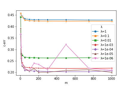
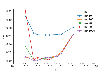
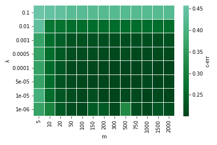
Figure 1: The graphs above are obtained from SUSY data set: on the left we show how c-err measure changes for different choices of $\lambda$ parameter; in the central figure the focus is on the stability of the algorithm varying $\lambda$; on the right the combined behavior is presented with a heatmap.

Table 2: Architecture: single machine with AMD EPYC 7301 16-Core Processor and 256GB of RAM. For Nyström-Pegaos, ALS sampling has been used [Rudi et al., (2018)] and the results are reported as mean and standard deviation deriving from 5 independent runs of the algorithm. The columns of the table report classification error, training time and prediction time (in seconds).

	LinSVM	KSVM			Nyström-Pegasos
Datasets	c-err	c-err	t train	t pred	c-err	t train	t pred	$m$
SUSY	$28.1\%$	-	-	-	$20.0\%\pm 0.2\%$	$608\pm 2$	$134\pm 4$	$2500$
Mnist bin	$12.4\%$	$2.2\%$	$1601$	$87$	$2.2\%\pm 0.1\%$	$1342\pm 5$	$491\pm 32$	$15000$
Usps	$16.5\%$	$3.1\%$	$4.4$	$1.0$	$3.0\%\pm 0.1\%$	$19.8\pm 0.1$	$7.3\pm 0.3$	$2500$
Webspam	$8.8\%$	$1.1\%$	$6044$	$473$	$1.3\%\pm 0.1\%$	$2440\pm 5$	$376\pm 18$	$11500$
a9a	$16.5\%$	$15.0\%$	$114$	$31$	$15.1\%\pm 0.2\%$	$29.3\pm 0.2$	$1.5\pm 0.1$	$800$
CIFAR	$31.5\%$	$19.1\%$	$6339$	$213$	$19.2\%\pm 0.1\%$	$2408\pm 14$	$820\pm 47$	$20500$

As mentioned in the introduction, a main of motivation for our study is showing that the computational savings can be achieved without incurring in any loss of accuracy. In this section, we complement our theoretical results investigating numerically the statistical and computational trade-offs in a relevant setting. More precisely, we report simple experiments in the context of kernel methods, considering Nyström techniques. In particular, we choose the hinge loss, hence SVM for classification. Keeping in mind Theorem 3 we expect we can match the performances of kernel-SVM using a Nyström approximation with only $m\ll n$ centers. The exact number depends on assumptions, such as the eigen-decay of the covariance operator, that might be hard to know in practice, so here we explore this empirically.

Nyström-Pegasos. Classic SVM implementations with hinge loss are based on considering a dual formulation and a quadratic programming problem [Joachims, (1998)]. This is the case for example, for the LibSVM library [Chang and Lin, (2011)] available on Scikit-learn [Pedregosa et al., (2011)]. We use this implementation for comparison, but find it convenient to combine the Nyström method to a primal solver akin to (6) (see Li et al., (2016); Hsieh et al., (2014) for the dual formulation). More precisely, we use Pegasos [Shalev-Shwartz et al., (2011)] which is based on a simple and easy to use stochastic subgradient iteration. We consider a procedure in two steps. First, we compute the embedding discussed in Section 3. With kernels it takes the form ${\mathbb{x}}_{i}=(K_{m}^{\dagger})^{1/2}(K(x_{i},\tilde{x}_{1}),\dots,K(x_{i},\tilde{x}_{m}))^{T},$ where $K_{m}\in\mathbb{R}^{m\times m}$ with $(K_{m})_{ij}=K(\tilde{x}_{i},\tilde{x}_{j})$. Second, we use Pegasos on the embedded data. As discussed in Section 3, the total cost is $O(nm^{2}C_{K}+nm\cdot\#iter)$ in time (here $\text{iter}=\text{epoch}$, i.e. one epoch equals $n$ steps of stochastic subgradient) and $O(m^{2})$ in memory (needed to compute the pseudo-inverse and embedding the data in batches of size $m$).
Datasets & set up (see Appendix J). We consider five datasets of size $10^{4}-10^{6}$, challenging for standard SVMs. We use a Gaussian kernel, tuning width and regularization parameter as explained in appendix. We report classification error and for data sets with no fixed test set, we set apart $20\%$ of the data.
Procedure Given the accuracy achieved by K-SVM algorithm, we increase the number of sampled Nyström points $m<n$ as long as also Nyström-Pegasos matches that result.
Results We compare with linear (used only as baseline) and K-SVM see Table 2. For all the datasets, the Nyström-Pegasos approach achieves comparable performances of K-SVM with much better time requirements (except for the small-size Usps). Moreover, note that K-SVM cannot be run on millions of points (SUSY), whereas Nyström-Pegasos is still fast and provides much better results than linear SVM. Further comparisons with state-of-art algorithms for SVM are left for a future work. Finally, in Figure 1 we illustrate the interplay between $\lambda$ and $m$ for the Nyström-Pegasos considering SUSY data set.

6 Conclusions

In this paper, we extended results for square loss [Rudi et al., (2015)] and self-concordant loss functions such as logistic loss [Marteau-Ferey et al., (2019)] to convex Lipschitz non-smooth loss functions such as hinge loss. The main idea is to save computations by solving the regularized ERM problem in a random subspace of the hypothesis space. We analysed the specific case of Nyström, where a data dependent subspace spanned by a random subset of the data is considered. In this setting we proved that under proper assumptions there is no statistical-computational tradeoff and our excess risk bounds can still match state-of-art results for SVM’s [Steinwart and Christmann, (2008)]. In particular, to achieve this behaviour we need sub-gaussianity of the input variables, a polynomial decay of the spectrum of the covariance operator and leverage scores sampling of the data. Theoretical guarantees have been proven both in the realizable case and, introducing the approximation error $\mathcal{A}(\lambda)$, when $w_{*}$ does not exists. Numerical simulations using real data seem to support our theoretical findings while providing the desired computational savings. The obtained results can match the ones for random features [Sun et al., (2018)], but also allow to reach faster rates with more Nyström points while the others saturate. We leave for a longer version of the paper a unified analysis which includes square and logistic losses as special cases, and the consequences for classification.

Appendix A Notation

For reader’s convenience we collect the main notation we introduced in the paper.

Notation: We denote with the “hat”, e.g. $\widehat{w}$, random quantities depending on the data. Given a linear operator $A$ we denote by $A^{\top}$ its adjoint (transpose for matrices). For any $n\in\mathbb{N}$, we denote by $\left\langle,\right\rangle_{n},\left\|\right\|_{n}$ the inner product and norm in $\mathbb{R}^{n}$. Given two quantities $a,b$ (depending on some parameters), the notation $a\lesssim b$, or $a=O(b)$ means that there exists constant such that $a\leqslant Cb$.

Table 3: Definition of the main quantities used in the paper

	Definition
$L(w)$	$\;\int_{\mathcal{H}\times\mathcal{Y}}\ell({y},\left\langle w,{x}\right\rangle)dP(x,y)$
$L_{\lambda}(w)$	$\;L(w)+\lambda\|w\|^{2}$
$\widehat{L}(w)$	$\;n^{-1}\sum_{i=1}^{n}\ell(y_{i},\left\langle w,x_{i}\right\rangle)$
$\widehat{L}_{\lambda}(w)$	$\;\widehat{L}(w)+\lambda\|w\|^{2}$
$w_{*}$	$\;\mathop{\mathrm{arg}\,\mathrm{min}}_{w\in\mathcal{H}}L(w)$
$w_{\lambda}$	$\;\mathop{\mathrm{arg}\,\mathrm{min}}_{w\in\mathcal{H}}L_{\lambda}(w)$
$\widehat{w}_{\lambda}$	$\;\mathop{\mathrm{arg}\,\mathrm{min}}_{w\in\mathcal{H}}\widehat{L}_{\lambda}(w)$
$\beta_{\lambda,{\cal B}}$	$\;\mathop{\mathrm{arg}\,\mathrm{min}}_{\beta\in{\cal B}}L_{\lambda}(\beta)$
$\widehat{\beta}_{\lambda,{\cal B}}$	$\;\mathop{\mathrm{arg}\,\mathrm{min}}_{\beta\in{\cal B}}\widehat{L}_{\lambda}(\beta)$
$f_{*}(x)$	$\;\mathop{\mathrm{arg}\,\mathrm{min}}_{a\in\mathbb{R}}\int_{\mathcal{Y}}\ell(y,a)dP(y|x)$
${\cal B}_{m}$	$\;{\cal B}_{m}=\text{span}\{\widetilde{x}_{1},\dots,\widetilde{x}_{m}\}$
$\mathcal{P}_{\cal B}$	proj operator onto ${\cal B}$
$\mathcal{P}_{m}$	proj operator onto ${\cal B}_{m}$

Appendix B Proof of Theorem 1

This section is devoted to the proof of Theorem 1. In the following we restrict to linear functions, i.e $f(x)=\left\langle w,x\right\rangle$ for some $w\in\mathcal{H}$ and, with slight abuse of notation we set

$$\ell(w,z)=\ell(y,\left\langle w,x\right\rangle),\qquad z=(x,y)\in\mathcal{H}\times\mathcal{Y},\ w\in\mathcal{H}.$$

With this notation $L(w)=\int_{\mathcal{H}\times\mathcal{Y}}\ell(w,z)dP(z)$. The Lipschitz assumption implies that $\ell(\cdot,(X,Y))$ is almost surely Lipschitz in its argument, with Lipschitz constant $G\kappa$.

Specifically, we will show the following:

Theorem 6.

Under Assumptions 1, 2, for $\lambda>0$ and $\delta\in(0,1)$ let

$$C_{\lambda,\delta}=4\big{\{}1+\sqrt{\log(1+\log_{2}(3+{\ell_{0}\kappa^{2}/\lambda}))+\log(2/\delta)}\big{\}}=O(\sqrt{\log\log(3+\ell_{0}\kappa^{2}/\lambda)+\log(1/\delta)}).$$

If Assumption 3 holds, then with probability $1-\delta$,

$$L(\widehat{w}_{\lambda})<\inf_{\mathcal{H}}L+\lambda\|w_{*}\|^{2}+\frac{C_{\lambda,\delta}^{2}G^{2}\kappa^{2}}{4\lambda n}+\frac{GC_{\lambda,\delta}}{\sqrt{n}}+(\ell_{0}+G\kappa\|w_{*}\|)\sqrt{\frac{2\log(2/\delta)}{n}}.$$ (27)

More generally, with probability $1-\delta$, letting $\mathcal{A}(\lambda):=\inf_{w\in\mathcal{H}}L(w)+\lambda\|w\|^{2}-\inf_{w\in\mathcal{H}}L(w)$,

$$L(\widehat{w}_{\lambda})-\inf_{\mathcal{H}}L<2\mathcal{A}(\lambda)+\frac{C_{\lambda,\delta}^{2}G^{2}\kappa^{2}+8G^{2}\kappa^{2}\log(2/\delta)}{4\lambda n}+\frac{GC_{\lambda,\delta}}{\sqrt{n}}+\ell_{0}\sqrt{\frac{2\log(2/\delta)}{n}}$$ (28)

$$\leqslant 2\Big{(}\inf_{\|w\|\leqslant R}L(w)-\inf_{\mathcal{H}}L\Big{)}+2\lambda R^{2}+\frac{C_{\lambda,\delta}^{2}G^{2}\kappa^{2}+8G^{2}\kappa^{2}\log(2/\delta)}{4\lambda n}+\frac{GC_{\lambda,\delta}+\ell_{0}\sqrt{2\log(2/\delta)}}{\sqrt{n}}$$

for every $R>0$.

The proof starts with the following bound on the generalization gap $L(w)-\widehat{L}(w)$ uniformly over balls. While this result is well-known and follows from standard arguments (see, e.g., Bartlett and Mendelson, (2002); Koltchinskii, (2011)), we include a short proof for completeness.

Lemma 1.

Under Assumptions 1 and 2 and, for every $R>0$, one has with probability at least $1-\delta$,

$$\sup_{\|w\|\leqslant R}\big{[}L(w)-\widehat{L}(w)\big{]}<\frac{GR\kappa}{\sqrt{n}}\Big{(}2+\sqrt{2\log(1/\delta)}\Big{)}.$$ (29)

Proof of Lemma 1.

The proof starts by a standard symmetrization step [Giné and Zinn, (1984); Koltchinskii, (2011)]. Let us call ${D}:=(z_{1},\dots,z_{n})$ i.i.d. from $P$, as well as an independent ${D}^{\prime}:=(z_{1}^{\prime},\dots,z_{n}^{\prime})$ i.i.d. from $P$ and $\varepsilon_{1},\dots,\varepsilon_{n}$ i.i.d. with $\mathbb{P}(\varepsilon_{i}=1)=\mathbb{P}(\varepsilon_{i}=-1)=1/2$. We denote $\widehat{L}^{\prime}(w):=n^{-1}\sum_{i=1}^{n}\ell(w,z_{i}^{\prime})$ the error on the sample $D^{\prime}$. Then,

$$\mathbb{E}_{D\sim P^{n}}\sup_{\|w\|\leqslant R}\Big{[}L(w)-\widehat{L}(w)\Big{]} =\mathbb{E}_{D}\sup_{\|w\|\leqslant R}\Big{[}\mathbb{E}_{D^{\prime}}\widehat{L}^{\prime}(w)-\widehat{L}(w)\Big{]}$$

$$\leqslant\mathbb{E}_{D,D^{\prime}}\sup_{\|w\|\leqslant R}\Big{[}\widehat{L}^{\prime}(w)-\widehat{L}(w)\Big{]}$$

$$=\mathbb{E}_{D,D^{\prime},\varepsilon}\sup_{\|w\|\leqslant R}\Big{[}\frac{1}{n}\sum_{i=1}^{n}\varepsilon_{i}\big{(}\ell(w,z_{i})-\ell(w,z_{i}^{\prime})\big{)}\Big{]}$$

$$=2\mathbb{E}_{D,\varepsilon}\bigg{[}\sup_{\|w\|\leqslant R}\frac{1}{n}\sum_{i=1}^{n}\varepsilon_{i}\ell(w,z_{i})\bigg{]}$$

where we used that $\mathbb{E}_{{D}^{\prime}}\widehat{L}^{\prime}(\cdot)=L(\cdot)$, and that $(\ell(f,z_{i})-\ell(f,z^{\prime}_{i}))_{1\leqslant i\leqslant n}$ and $(\varepsilon_{i}(\ell(f,z_{i})-\ell(f,z^{\prime}_{i})))_{1\leqslant i\leqslant n}$ have the same distribution, as well as $(\varepsilon_{i}\ell(f,z_{i}))_{i}$ and $(-\varepsilon_{i}\ell(f,z^{\prime}_{i}))_{i}$. The last term corresponds to the Rademacher complexity of the class of functions $\{\ell(w,\cdot):\|w\|\leqslant R\}$ [Bartlett and Mendelson, (2002); Koltchinskii, (2011)]. Now, using that $\ell(w,z_{i})=\ell(y_{i},\langle w,x_{i}\rangle)$ for $z_{i}=(x_{i},y_{i})$, where $\ell(y_{i},\cdot)$ is $G$-Lipschitz by Assumption 2, Ledoux-Talagrand’s contraction inequality for Rademacher averages [Meir and Zhang, (2003)] gives

$$\mathbb{E}_{D,\varepsilon}\bigg{[}\sup_{\|w\|\leqslant R}\frac{1}{n}\sum_{i=1}^{n}\varepsilon_{i}\ell(w,z_{i})\bigg{]} \leqslant G\mathbb{E}_{D,\varepsilon}\bigg{[}\sup_{\|w\|\leqslant R}\frac{1}{n}\sum_{i=1}^{n}\varepsilon_{i}\langle w,x_{i}\rangle\bigg{]}$$

$$=G\mathbb{E}_{D,\varepsilon}\bigg{[}\sup_{\|w\|\leqslant R}\Big{\langle}w,\frac{1}{n}\sum_{i=1}^{n}\varepsilon_{i}x_{i}\Big{\rangle}\bigg{]}$$

$$\leqslant GR\mathbb{E}_{D,\varepsilon}\bigg{[}\Big{\|}\frac{1}{n}\sum_{i=1}^{n}\varepsilon_{i}x_{i}\Big{\|}^{2}\bigg{]}^{1/2}$$

$$=\frac{GR\mathbb{E}[\|x\|^{2}]^{1/2}}{\sqrt{n}}$$

$$\leqslant\frac{GR\kappa}{\sqrt{n}}$$

where we used that $\mathbb{E}[\varepsilon_{i}\varepsilon_{j}\langle x_{i},x_{j}\rangle]=0$ for $i\neq j$ by independence, and that $\|x\|\leqslant\kappa$ almost surely (Assumption 1). Hence,

$$\mathbb{E}_{D\sim P^{n}}\sup_{\|w\|\leqslant R}\Big{[}L(w)-\widehat{L}(w)\Big{]}\leqslant\frac{2GR\kappa}{\sqrt{n}}.$$ (30)

To write the analogous bound in high probability we apply McDiarmid’s inequality [Boucheron et al., (2013)]. We know that given ${D}:=\{z_{1},\dots,z_{i},\dots,z_{n}\}$, ${D}^{i}=\{z_{1},\dots,z^{\prime}_{i},\dots,z_{n}\}$ and defining $\phi({D}):=\sup_{\|w\|\leqslant R}[L(w)-\widehat{L}(w)]$ we have

$$\Big{|}\phi({D})-\phi({D}^{i})\Big{|} \leqslant\sup_{\|w\|\leqslant R}\Big{|}\frac{1}{n}\ell(w,z_{i})-\frac{1}{n}\ell(w,z^{\prime}_{i})\Big{|}$$

$$\leqslant\frac{G}{n}\sup_{\|w\|\leqslant R}\Big{|}\langle w,x_{i}-x_{i}^{\prime}\rangle\Big{|}$$

$$\leqslant\frac{2GR\kappa}{n}$$ (31)

using the Assumption 1 of boundedness of the input. Hence, by McDiarmid inequality:

$$\mathbb{P}\Big{[}\phi({D})-\mathbb{E}_{D}[\phi({D})]\geqslant t\Big{]}\leqslant\exp\Big{(}\frac{-t^{2}n}{2G^{2}R^{2}\kappa^{2}}\Big{)};$$ (32)

taking $\delta=\exp\Big{(}\frac{-t^{2}n}{2G^{2}R^{2}\kappa^{2}}\Big{)}$ so that $t=GR\kappa\sqrt{\frac{2\log(1/\delta)}{n}}$, we obtain the desired bound (29). ∎

Lemma 1 suffices to control the excess risk of the constrained risk minimizer $\widehat{w}:=\mathop{\mathrm{arg}\,\mathrm{min}}_{\|w\|\leqslant R}L(w)$ for $R=\|w_{*}\|$. On the other hand, this result cannot be readily applied to $\widehat{w}_{\lambda}$, since its norm $\|\widehat{w}_{\lambda}\|$ is itself random. Observe that, by definition and by Assumption 2,

$$\lambda\|\widehat{w}_{\lambda}\|^{2}\leqslant\widehat{L}_{\lambda}(\widehat{w}_{\lambda})\leqslant\widehat{L}_{\lambda}(0)=\widehat{L}(0)\leqslant\sup_{y\in\mathcal{Y}}\ell(y,0)=\ell_{0},$$

so that $\|\widehat{w}_{\lambda}\|\leqslant\sqrt{\ell_{0}/\lambda}$. One could in principle apply this bound on $\widehat{w}_{\lambda}$, but this would yield a suboptimal dependence on $\lambda$ and thus a suboptimal rate.

The next step in the proof is to make the bound of Lemma 1 valid for all norms $R$, so that it can be applied to the random quantity $R=\|\widehat{w}_{\lambda}\|$. This is done in Lemma 2 below though a union bound.

Lemma 2.

Under Assumptions 1 and 2, with probability $1-\delta$, one has:

$$\forall w\in\mathcal{H},\qquad L(w)-\widehat{L}(w)\leqslant\frac{4G(1+\kappa\|w\|)}{\sqrt{n}}\Big{(}1+\sqrt{\log(2+\log_{2}(1+\kappa\|w\|))+\log(1/\delta)}\Big{)}.$$

Proof of Lemma 2.

Fix $\delta\in(0,1)$. For $p\geqslant 1$, let $R_{p}:=\kappa^{-1}2^{p}$ and $\delta_{p}=\delta/(p(p+1))$. By Lemma 1, one has for every $p\geqslant 1$,

$$\mathbb{P}\Bigg{(}\sup_{\|w\|\leqslant R_{p}}\Big{[}L(w)-\widehat{L}(w)\Big{]}\geqslant\frac{G\kappa R_{p}}{\sqrt{n}}\Big{(}2+\sqrt{2\log\frac{1}{\delta_{p}}}\Big{)}\Bigg{)}\leqslant\delta_{p}.$$

Taking a union bound over $p\geqslant 1$ and using that $\sum_{p\geqslant 1}\delta_{p}=\delta$ and $\delta_{p}\geqslant\delta^{2}/(p+1)^{2}$, we get:

$$\mathbb{P}\Bigg{(}\exists p\geqslant 1,\quad\sup_{\|w\|\leqslant R_{p}}\Big{[}L(w)-\widehat{L}(w)\Big{]}\geqslant\frac{G\kappa R_{p}}{\sqrt{n}}\Big{(}2+2\sqrt{\log\frac{p+1}{\delta}}\Big{)}\Bigg{)}\leqslant\delta.$$

Now, for $w\in\mathcal{H}$, let $p=\lceil\log_{2}(1+\kappa\|w\|)\rceil$; then, $1+\kappa\|w\|\leqslant\kappa R_{p}=2^{p}\leqslant 2(1+\kappa\|w\|)$, so $\|w\|\leqslant R_{p}$. Hence, with probability $1-\delta$,

$$\forall w\in\mathcal{H},\qquad L(w)-\widehat{L}(w)\leqslant\frac{4G(1+\kappa\|w\|)}{\sqrt{n}}\Big{(}1+\sqrt{\log\big{(}2+\log_{2}(1+\kappa\|w\|)\big{)}+\log(1/\delta)}\Big{)}.$$

This is precisely the desired bound. ∎

Since the bound of Lemma 2 holds simultaneously for all $w\in\mathcal{H}$, one can apply it to $\widehat{w}_{\lambda}$; using the inequality $\kappa\|\widehat{w}_{\lambda}\|\leqslant\kappa\sqrt{\ell_{0}/\lambda}\leqslant(1+\ell_{0}\kappa^{2}/\lambda)/2$ to bound the $\log\log$ term, this gives with probability $1-\delta$,

$$L(\widehat{w}_{\lambda})-\widehat{L}(\widehat{w}_{\lambda})\leqslant\frac{4G(1+\kappa\|\widehat{w}_{\lambda}\|)}{\sqrt{n}}\Big{(}1+\sqrt{\log\big{(}1+\log_{2}(3+{\ell_{0}\kappa^{2}/\lambda})\big{)}+\log(1/\delta)}\Big{)}.$$ (33)

Now, let $C=C_{\lambda,\delta}=4\big{\{}1+\sqrt{\log(1+\log_{2}(3+{\ell_{0}\kappa^{2}/\lambda}))+\log(1/\delta)}\big{\}}$; (33) writes $L(\widehat{w}_{\lambda})-\widehat{L}(\widehat{w}_{\lambda})\leqslant CG(1+\kappa\|\widehat{w}_{\lambda}\|)/\sqrt{n}$. Using that $ab\leqslant\lambda a^{2}+b^{2}/(4\lambda)$ for $a,b\geqslant 0$, one can then write

$$L(\widehat{w}_{\lambda}) \leqslant\widehat{L}(\widehat{w}_{\lambda})+\frac{CG\kappa\|\widehat{w}_{\lambda}\|}{\sqrt{n}}+\frac{CG}{\sqrt{n}}$$

$$\leqslant\widehat{L}(\widehat{w}_{\lambda})+\lambda\|\widehat{w}_{\lambda}\|^{2}+\frac{C^{2}G^{2}\kappa^{2}}{4\lambda n}+\frac{CG}{\sqrt{n}}$$ (34)

$$\leqslant\widehat{L}(w_{\lambda})+\lambda\|w_{\lambda}\|^{2}+\frac{C^{2}G^{2}\kappa^{2}}{4\lambda n}+\frac{CG}{\sqrt{n}}$$ (35)

where (35) holds by definition of $\widehat{w}_{\lambda}$. Now, since $|\ell(w_{\lambda},Z)|\leqslant|\ell(Y,0)|+|\ell(Y,\langle w_{\lambda},X\rangle)-\ell(Y,0)|\leqslant\ell_{0}+G\kappa\|w_{\lambda}\|$ almost surely, Hoeffding’s inequality [Boucheron et al., (2013)] implies that, with probability $1-\delta$,

$$\widehat{L}(w_{\lambda})<L(w_{\lambda})+(\ell_{0}+G\kappa\|w_{\lambda}\|)\sqrt{\frac{2\log(1/\delta)}{n}}.$$

Combining this inequality with (35) with a union bound, with probability $1-2\delta$:

$$L(\widehat{w}_{\lambda})<L(w_{\lambda})+\lambda\|w_{\lambda}\|^{2}+\frac{C^{2}G^{2}\kappa^{2}}{4\lambda n}+\frac{GC}{\sqrt{n}}+(\ell_{0}+G\kappa\|w_{\lambda}\|)\sqrt{\frac{2\log(1/\delta)}{n}}.$$ (36)

First case: $w_{*}$ exists.

First, assume that $w_{*}=\mathop{\mathrm{arg}\,\mathrm{min}}_{w\in\mathcal{H}}L(w)$ exists. Then, by definition of $w_{\lambda}$, $L(w_{\lambda})+\lambda\|w_{\lambda}\|^{2}\leqslant L(w_{*})+\lambda\|w_{*}\|^{2}$. In addition, $\|w_{\lambda}\|\leqslant\|w_{*}\|$, since otherwise $\|w_{*}\|<\|w_{\lambda}$ and $L(w_{*})\leqslant L(w_{\lambda})$ would imply $L(w_{*})+\lambda\|w_{*}\|^{2}<L(w_{\lambda})+\lambda\|w_{\lambda}\|^{2}$, contradicting the above inequality. Since $L(w_{*})=\inf_{\mathcal{H}}L$, it follows that, with probability $1-2\delta$,

$$L(\widehat{w}_{\lambda}) <\inf_{\mathcal{H}}L+\lambda\|w_{*}\|^{2}+\frac{C^{2}G^{2}\kappa^{2}}{4\lambda n}+\frac{GC}{\sqrt{n}}+(\ell_{0}+G\kappa\|w_{*}\|)\sqrt{\frac{2\log(1/\delta)}{n}}$$

$$\leqslant\inf_{\mathcal{H}}L+\lambda\|w_{*}\|^{2}+\frac{8G^{2}\kappa^{2}\big{\{}1+{\log(1+\log_{2}(3+{\ell_{0}\kappa^{2}/\lambda}))+\log(1/\delta)}\big{\}}}{\lambda n}+$$

$$+\frac{4G\big{\{}1+\sqrt{\log(1+\log_{2}(3+{\ell_{0}\kappa^{2}/\lambda}))+\log(1/\delta)}\big{\}}}{\sqrt{n}}+(\ell_{0}+G\kappa\|w_{*}\|)\sqrt{\frac{2\log(1/\delta)}{n}}$$

$$=\inf_{\mathcal{H}}L+O\Big{(}\lambda\|w_{*}\|^{2}+\frac{G^{2}\kappa^{2}\{\log\log(3+\ell_{0}\kappa^{2}/\lambda)+\log(1/\delta)\}}{\lambda n}+\frac{(G+\ell_{0})\sqrt{\log(1/\delta)}}{\sqrt{n}}\Big{)},$$ (37)

where the $O(\dots)$ hide universal constants. The bound (B) precisely corresponds to the desired bound (27) after replacing $\delta$ by $\delta/2$. In particular, tuning $\lambda\asymp(G\kappa/\|w_{*}\|)\sqrt{\log(1/\delta)/n}$ yields

$$L(\widehat{w}_{\lambda})-\inf_{\mathcal{H}}L\lesssim\frac{\{\ell_{0}+G(1+\kappa\|w_{*}\|)\}\{\log\log(\kappa\|w_{*}\|n/G)+\sqrt{\log(1/\delta)}\}}{\sqrt{n}}.$$

Omitting the $\log\log n$ term, this bound essentially scales as $\widetilde{O}(G\kappa\|w_{*}\|\sqrt{\log(1/\delta)/n})$.

General case.

Let us now drop the assumption that $w_{*}=\mathop{\mathrm{arg}\,\mathrm{min}}_{w\in\mathcal{H}}L(w)$ exists, and let (see (24)) for $\lambda>0$:

$$\mathcal{A}(\lambda) =L(w_{\lambda})+\lambda\|w_{\lambda}\|^{2}-\inf_{\mathcal{H}}L$$

$$=\inf_{w\in\mathcal{H}}[L(w)+\lambda\|w\|^{2}]-\inf_{\mathcal{H}}L\,.$$

Note that, again using that $ab\leqslant\lambda a^{2}+b^{2}/(4\lambda)$,

$$G\kappa\|w_{\lambda}\|\sqrt{\frac{2\log(1/\delta)}{n}} \leqslant\lambda\|w_{\lambda}\|^{2}+\frac{2G^{2}\kappa^{2}\log(1/\delta)}{\lambda n}$$

$$\leqslant\mathcal{A}(\lambda)+\frac{2G^{2}\kappa^{2}\log(1/\delta)}{\lambda n}$$

so that (36) implies, with probability $1-2\delta$,

$$L(\widehat{w}_{\lambda})-\inf_{\mathcal{H}}L<2\mathcal{A}(\lambda)+\frac{C^{2}G^{2}\kappa^{2}}{4\lambda n}+\frac{GC}{\sqrt{n}}+$$

$$\hskip 85.35826pt\ell_{0}\sqrt{\frac{2\log(1/\delta)}{n}}+\frac{2G^{2}\kappa^{2}\log(1/\delta)}{\lambda n}.$$

Finally, note that for all $w\in\mathcal{H}$ with $\|w\|\leqslant R$, $\mathcal{A}(\lambda)\leqslant L(w)+\lambda\|w\|^{2}-\inf_{\mathcal{H}}L\leqslant L(w)-\inf_{\mathcal{H}}L+\lambda R^{2}$, hence $\mathcal{A}(\lambda)\leqslant\inf_{\|w\|\leqslant R}L(w)-\inf_{\mathcal{H}}L+\lambda R^{2}$ and

$$L(\widehat{w}_{\lambda})-\inf_{\mathcal{H}}L<2\Big{(}\inf_{\|w\|\leqslant R}L(w)-\inf_{\mathcal{H}}L\Big{)}+2\lambda R^{2}+$$

$$\hskip 19.91684pt\frac{C^{2}G^{2}\kappa^{2}+8G^{2}\kappa^{2}\log(1/\delta)}{4\lambda n}+\frac{GC+\ell_{0}\sqrt{2\log(1/\delta)}}{\sqrt{n}}.$$

Letting $\lambda\asymp 1/(R\sqrt{n})$, this gives $L(\widehat{w}_{\lambda})-\inf_{\mathcal{H}}L\leqslant 2(\inf_{\|w\|\leqslant R}L(w)-\inf_{\mathcal{H}}L)+O(R/\sqrt{n})$ with high probability.

Appendix C Proof of Theorem 2

The proof of Theorem 2 is given by decomposing the excess risk as in (E) where $\mathcal{P}_{m}$ is replaced by $\mathcal{P}_{{\cal B}}$, (47) bounds term A, (48) bounds term B and (E) and the Definition 14 bound term C.

Appendix D $T$-approximate leverage scores and proof of Proposition 1

Since in practice the leverage scores $l_{i}(\alpha)$ defined by (10) are onerous to compute, approximations $(\hat{l}_{i}(\alpha))_{i=1}^{n}$ have been considered [Drineas et al., (2012); Cohen et al., (2015); Alaoui and Mahoney, (2015)]. In particular, in the following we are interested in suitable approximations defined as follows.

Definition 2.

($T$-approximate leverage scores) Let $(l_{i}(\alpha))_{i=1}^{n}$ be the leverage scores associated to the training set for a given $\alpha$. Let $\delta>0$, $t_{0}>0$ and $T\geqslant 1$. We say that $(\hat{l}_{i}(\alpha))_{i=1}^{n}$ are $T$-approximate leverage scores with confidence $\delta$, when with probability at least $1-\delta$,

$$\frac{1}{T}l_{i}(\alpha)\leqslant\hat{l}_{i}(\alpha)\leqslant Tl_{i}(\alpha),\hskip 17.07182pt\forall i\in\{1,\dots,n\},\;\;\alpha\geqslant t_{0}$$ (38)

So, given $T$-approximate leverage score for $\alpha\geqslant t_{0}$, $\{\tilde{x}_{1},\dots,\tilde{x}_{m}\}$ are sampled from the training set independently with replacement, and with probability to be selected given by $Q_{\alpha}(i)=\hat{l}_{i}(\alpha)/\sum_{j}\hat{l}_{j}(\alpha)$.

First part of Proposition 1 is the content of the following two results from Rudi et al., (2015).

Lemma 3 (Uniform sampling, Lemma 6 in Rudi et al., (2015)).

Under Assumption 1, let $J$ be a partition of $\{1,\dots,n\}$ chosen uniformly at random from the partitions of cardinality $m$. Let $\alpha>0$, for any $\delta>0$, such that $m\geqslant 67\log\frac{4\kappa^{2}}{\alpha\delta}\vee 5d_{\alpha,\infty}\log\frac{4\kappa^{2}}{\alpha\delta}$, the following holds with probability at least $1-\delta$

$$\Big{\|}(I-{\mathcal{P}}_{{\cal B}_{m}})\Sigma^{1/2}\Big{\|}^{2}\leqslant 3\alpha$$ (39)

Lemma 4 (ALS sampling, Lemma 7 in Rudi et al., (2015)).

Let $(\hat{l}_{i}(t))_{i=1}^{n}$ be the collection of approximate leverage scores. Let $\alpha>0$ and the sampling probability $Q_{\alpha}$ be defined as $Q_{\alpha}(i)=\hat{l}_{i}(\alpha)/\sum_{j\in N}\hat{l}_{j}(\alpha)$ for any $i\in N$ with $N=\{1,...,n\}$. Let $\mathcal{I}=(i_{1},...,i_{m})$ be a collection of indices independently sampled with replacement from $N$ according to the probability distribution $P_{\alpha}$. Let ${\cal B}_{m}=\text{span}\{x_{j}|j\in J\}$ where $J$ be the subcollection of $\mathcal{I}$ with all the duplicates removed. Under Assumption 1, for any $\delta>0$ the following holds with probability at least $1-\delta$

$$\Big{\|}(I-{\mathcal{P}}_{{\cal B}_{m}})\Sigma_{\alpha}^{1/2}\Big{\|}^{2}\leqslant 3\alpha$$ (40)

where the following conditions are satisfied:

1. there exists a $T\geqslant 1$ and a $t_{0}>0$ such that $(l_{i}(t))_{i=1}^{n}$ are $T$-approximate leverage scores for any $t\geqslant t_{0}$,

2. $n\geqslant 1655\kappa^{2}+223\kappa^{2}\log\frac{4\kappa^{2}}{\delta}$,

3. $t_{0}\vee\frac{19\kappa^{2}}{n}\log\frac{4n}{\delta}\leqslant\alpha\leqslant\|\Sigma\|$,

4. $m\geqslant 334\log\frac{16n}{\delta}\vee 78T^{2}d_{\alpha,2}\log\frac{16n}{\delta}$.

If the spectrum of $\Sigma$ satisfies the decay property (15), the second part of Proposition 1 is a consequence of Lemma 4.

Appendix E Proof of Theorem 3

Theorem 3 is a compact version of the following result.

Theorem 7.

Fix $\alpha,\lambda,\delta>0$. Under Assumption 1, 2 and  3, with probability at least $1-\delta$:

$$L(\widehat{\beta}_{\lambda})-L(w_{*}) \leqslant\frac{C^{2}_{\lambda,\delta}G^{2}\kappa^{2}}{4\lambda n}+\frac{C_{\lambda,\delta}G}{\sqrt{n}}+G\kappa\|w_{*}\|\sqrt{\frac{2\log(3/\delta)}{n}}+2G\sqrt{\alpha}\|w_{*}\|+\lambda\|w_{*}\|^{2}_{\mathcal{H}}$$ (41)

$$C_{\lambda,\delta} =4\big{\{}1+\sqrt{\log(1+\log_{2}(3+{\ell_{0}\kappa^{2}/\lambda}))+\log(1/\delta)}\big{\}}$$

provided that $n\geqslant 1655\kappa^{2}+223\kappa^{2}\log\frac{4\kappa^{2}}{\delta}$ and

1. for uniform sampling

   $$m\geqslant 67\log\frac{4\kappa^{2}}{\alpha\delta}\vee 5d_{\alpha,\infty}\log\frac{4\kappa^{2}}{\alpha\delta}$$ (42)

2. for ALS sampling and $T$-approximate leverage scores with subsampling probabilities $Q_{\alpha}$, $t_{0}>\frac{19\kappa^{2}}{n}\log\frac{4n}{\delta}$ and

   $$m\geqslant 334\log\frac{16n}{\delta}\vee 78T^{2}d_{\alpha,2}\log\frac{16n}{\delta}$$ (43)

   where $\alpha\geqslant\frac{19\kappa^{2}}{n}\log\frac{4n}{\delta}$

Proof.

We recall the notation.

$$\{\tilde{x}_{1},\dots,\tilde{x}_{m}\}\subseteq\{x_{1},\dots,x_{n}\}$$

$${\cal B}_{m}=\text{span}\{\tilde{x}_{1},\dots,\tilde{x}_{m}\}$$

$$\widehat{\beta}_{\lambda}=\mathop{\mathrm{arg}\,\mathrm{min}}_{w\in{\cal B}_{m}}\widehat{L}(w)$$

$$w_{*}=\mathop{\mathrm{arg}\,\mathrm{min}}_{w\in\mathcal{H}}\widehat{L}_{\lambda}(w).$$

and ${\mathcal{P}}_{m}=\mathcal{P}_{{\cal B}_{m}}$ is the orthogonal projector operator onto ${\cal B}_{m}$.
In order to bound the excess risk of $\widehat{\beta}_{\lambda}$, we decompose the error as follows:

$$L(\widehat{\beta}_{\lambda})-L(w_{*}) =\underbrace{L(\widehat{\beta}_{\lambda})-\widehat{L}(\widehat{\beta}_{\lambda})-\lambda\|\widehat{\beta}_{\lambda}\|^{2}_{\mathcal{H}}}_{\textbf{{A}}}+\underbrace{\widehat{L}(\widehat{\beta}_{\lambda})+\lambda\|\widehat{\beta}_{\lambda}\|^{2}_{\mathcal{H}}-\widehat{L}(\mathcal{P}_{m}w_{*})-\lambda\|\mathcal{P}_{m}w_{*}\|^{2}_{\mathcal{H}}}_{\leqslant 0}+$$

$$\hskip 14.22636pt+\underbrace{\widehat{L}(\mathcal{P}_{m}w_{*})-L(\mathcal{P}_{m}w_{*})}_{\textbf{B}}+\underbrace{L(\mathcal{P}_{m}w_{*})-L(w_{*})}_{\textbf{C}}+\lambda\|\mathcal{P}_{m}w_{*}\|^{2}_{\mathcal{H}}$$ (44)

Bound for term A

To bound term A we apply Lemma 2 for $\widehat{\beta}_{\lambda}$ and we get with probability a least $1-\delta$

$$\forall\lambda\geqslant\frac{\ell_{0}\kappa^{2}}{n^{2K}},\hskip 28.45274ptL(\widehat{\beta}_{\lambda})\leqslant\widehat{L}(\widehat{\beta}_{\lambda})+\frac{C_{\lambda,\delta}G(1+\kappa\|\widehat{\beta}_{\lambda}\|)}{\sqrt{n}}$$ (45)

where $C_{\lambda,\delta}=4\big{\{}1+\sqrt{\log(1+\log_{2}(3+{\ell_{0}\kappa^{2}/\lambda}))+\log(1/\delta)}\big{\}}$. Now since $xy\leqslant\lambda x^{2}+y^{2}/(4\lambda)$, we can write

$$\frac{C_{\lambda,\delta}G\kappa\|\widehat{\beta}_{\lambda}\|}{\sqrt{n}}\leqslant\lambda\|\widehat{\beta}_{\lambda}\|^{2}+\frac{C^{2}_{\lambda,\delta}G^{2}\kappa^{2}}{4\lambda n}$$ (46)

hence,

$$L(\widehat{\beta}_{\lambda}) \leqslant\widehat{L}(\widehat{\beta}_{\lambda})+\lambda\|\widehat{\beta}_{\lambda}\|^{2}+\frac{C^{2}_{\lambda,\delta}G^{2}\kappa^{2}}{4\lambda n}+\frac{C_{\lambda,\delta}G}{\sqrt{n}}$$ (47)

Bound for term B

As regards term B, since $|\ell(\mathcal{P}_{m}w_{*},Z)-\ell(0,Z)|\leqslant G\kappa\|\mathcal{P}_{m}w_{*}\|\leqslant G\kappa\|w_{*}\|$, using Hoeffding’s inequality, we have with probability at least $1-\delta$

B $$\leqslant\Big{|}\widehat{L}(\mathcal{P}_{m}w_{*})-L(\mathcal{P}_{m}w_{*})\Big{|}\leqslant G\kappa\|w_{*}\|\sqrt{\frac{2\log(1/\delta)}{n}}$$ (48)

Bound for term C

Finally, term C can be rewritten as

C $$=L(\mathcal{P}_{m}w_{*})-L(w_{*})$$

$$\leqslant G\|\Sigma^{1/2}(I-\mathcal{P}_{m})w_{*}\|_{\mathcal{H}}$$

$$\leqslant G\|\Sigma^{1/2}(I-\mathcal{P}_{m})\|\|w_{*}\|_{\mathcal{H}}$$ (49)

We bound equation (E) using Lemma 3 for uniform sampling and Lemma 4 for ALS selection.
Putting the pieces together and noticing that $\lambda\|\mathcal{P}_{m}w_{*}\|^{2}_{\mathcal{H}}\leqslant\lambda\|w_{*}\|^{2}_{\mathcal{H}}$ we finally get the result in Theorem 7. ∎

The following corollary shows that there is choice of the parameters $\lambda=\lambda_{n},\alpha=\alpha_{n}$ such that the excess risk of the $\beta_{\lambda_{n}}$ converges to zero with the optimal rate (up to a logarithmic factor) $O(\log(n/\delta)/\sqrt{n})$.

Corollary 1.

Fix $\delta>0$. Under the assumption of Theorem (7), let

$$\lambda\asymp\frac{1}{\|w_{*}\|}n^{-1/2}\qquad\alpha\asymp\frac{\log(n/\delta)}{n}$$

with probability at least $1-\delta$:

$$L(\widehat{\beta}_{\lambda})-L(w_{*})\lesssim\frac{\|w_{*}\|\sqrt{\log(n/\delta)}}{\sqrt{n}}$$ (50)

Despite of the fact that the rate is optimal (up to the logarithmic term), the required number of subsampled points is $m\gtrsim n\log n$, so that the procedure is not effective. However, the following proposition shows that under a fast decay for the spectrum of the covariance operator $\Sigma$, the ALS method becomes computationally efficient. We denote by $(\sigma_{i}(\Sigma))_{I}$ the sequence of strictly positive eigenvalues of $\Sigma$ where the eigenvalues are counted with respect to their multiplicity and ordered in a non-increasing way.

Proposition 2.

Fix $\delta>0$. Under the assumptions of Theorem (7) and using ALS sampling

1. for polynomial decay, i.e. $\sigma_{i}(\Sigma)\leqslant\gamma i^{-\frac{1}{p}}$, $\gamma\in\mathbb{R}^{+}$, $p\in(0,1)$, for $\delta>0$, with probability at least $1-\delta$:

   $$L(\widehat{\beta}_{\lambda})-L(w_{*})\leqslant\frac{C^{2}_{\lambda,\delta}G^{2}\kappa^{2}}{4\lambda n}+\frac{C_{\lambda,\delta}G}{\sqrt{n}}+G\kappa\|w_{*}\|\sqrt{\frac{2\log(3/\delta)}{n}}+2G\|w_{*}\|\sqrt{\alpha}+\lambda\|w_{*}\|^{2}_{\mathcal{H}}$$ (51)

   where $O(\sqrt{\frac{\log(n/\delta)}{n}})$ rate can be achieved optimizing the choice of the parameters, i.e. ${\lambda\asymp\frac{1}{\|w_{*}\|}n^{-1/2}}$, $\alpha\asymp\frac{\log(n/\delta)}{n}$, ${m\gtrsim n^{p}(\log n)^{1-p}}$.

2. for exponential decay, i.e. $\sigma_{i}(\Sigma)\leqslant\gamma e^{-\beta i}$, $\gamma,\beta\in\mathbb{R}^{+}$, for $\delta>0$, with probability at least $1-\delta$:

   $$L(\widehat{\beta}_{\lambda})-L(w_{*})\leqslant\frac{C^{2}_{\lambda,\delta}G^{2}\kappa^{2}}{4\lambda n}+\frac{C_{\lambda,\delta}G}{\sqrt{n}}+G\kappa\|w_{*}\|\sqrt{\frac{2\log(3/\delta)}{n}}+2G\|w_{*}\|\sqrt{\alpha}+\lambda\|w_{*}\|^{2}_{\mathcal{H}}$$ (52)

   where $O(\sqrt{\frac{\log(n/\delta)}{n}})$ rate can be achieved optimizing the choice of the parameter, i.e. ${\lambda\asymp\frac{1}{\|w_{*}\|}n^{-1/2}}$, ${\alpha\asymp\frac{\log(n/\delta)}{n}}$, $m\gtrsim\log^{2}n$.

Proof.

The claim is a consequence of Appendix H where the link with $m$ is obtained using Leverage Score sampling so that in Lemma 4 using proposition 4 we have that

$$m\gtrsim d_{\alpha,2}\log n,\hskip 28.45274ptd_{\alpha,2}\lesssim\alpha^{-p},\hskip 28.45274ptm\asymp n^{p}(\log n)^{1-p}$$ (53)

while using Proposition 5 we have that

$$m\gtrsim d_{\alpha,2}\log n,\hskip 28.45274ptd_{\alpha,2}\lesssim\log(1/\alpha),\hskip 28.45274ptm\asymp\log^{2}n$$ (54)

∎

From proposition above we have the following asymptotic rate.

Corollary 2.

Fix $\delta>0$. Under the assumptions of Theorem (7) and using ALS sampling, with probability at least $1-\delta$

1. assuming polynomial decay of the spectrum of $\Sigma$ and choosing $\lambda\asymp\frac{1}{\|w_{*}\|}n^{-1/2}$, ${m\gtrsim n^{p}(\log n)^{1-p}}$ then:

   $$L(\widehat{\beta}_{\lambda})-L(w_{*})\lesssim\frac{\|w_{*}\|\sqrt{\log(n/\delta)}}{\sqrt{n}}$$ (55)

2. assuming exponential decay of the spectrum of $\Sigma$ and choosing $\lambda\asymp\frac{1}{\|w_{*}\|}n^{-1/2}$, ${m\gtrsim\log^{2}n}$ then:

   $$L(\widehat{\beta}_{\lambda})-L(w_{*})\lesssim\frac{\|w_{*}\|\sqrt{\log(n/\delta)}}{\sqrt{n}}$$ (56)

Appendix F Proof of Theorem 4

Before proving Theorem 4 we introduce a modification of the above Lemma 4 in the case of sub-gaussian random variables

Lemma 5.

(ALS sampling for sub-gaussian variables). Let $(\hat{l}_{i}(t))_{i=1}^{n}$ be the collection of approximate leverage scores. Let $\alpha>0$ and the sampling probability $Q_{\alpha}$ be defined as $Q_{\alpha}(i)=\hat{l}_{i}(\alpha)/\sum_{j\in N}\hat{l}_{j}(\alpha)$ for any $i\in N$ with $N=\{1,...,n\}$. Let $\mathcal{I}=(i_{1},...,i_{m})$ be a collection of indices independently sampled with replacement from $N$ according to the probability distribution $P_{\alpha}$. Let ${\cal B}_{m}=\text{span}\{x_{j}|j\in J\}$ where $J$ be the subcollection of $\mathcal{I}$ with all the duplicates removed. Under Assumption 4, for any $\delta>0$ the following holds with probability at least $1-5\delta$

$$\Big{\|}(I-{\mathcal{P}}_{{\cal B}_{m}})\Sigma_{\alpha}^{1/2}\Big{\|}^{2}\lesssim\alpha$$ (57)

when the following conditions are satisfied:

1. there exists a $T\geqslant 1$ and a $t_{0}>0$ such that $(l_{i}(t))_{i=1}^{n}$ are $T$-approximate leverage scores for any $t\geqslant t_{0}$,

2. $$n\gtrsim d_{\alpha,2}(\Sigma)\vee\log(1/\delta)$$ (58)

3. $$m\gtrsim d_{\alpha,2}(\Sigma)\log(\frac{2n}{\delta})$$ (59)

Proof.

The proof follows the structure of the one in Lemma 4 (see Rudi et al., (2015)). Exploiting sub-gaussianity anyway the various terms are bounded differently. In particular, to bound $\beta_{1}$ we refer to Theorem 9 in Koltchinskii and Lounici, (2014), obtaining with probability at least $1-\delta$

$$\beta_{1}(\alpha)\lesssim\max\left\{\sqrt{\frac{d_{\alpha,2}(\Sigma)}{n}},\sqrt{\frac{\log(1/\delta)}{n}}\right\}.$$ (60)

As regards $\beta_{3}$ term we apply Proposition 3 below to get with probability greater than $1-3\delta$

$$\beta_{3}(\alpha)\leqslant\frac{2\log\frac{2n}{\delta}}{3m}+\sqrt{\frac{32T^{2}d_{\alpha,2}(\Sigma)\log\frac{2n}{\delta}}{m}}$$

for $n\geqslant 2C^{2}\log(1/\delta)$.
Finally, taking a union bound we have with probability at least $1-5\delta$

$$\beta(\alpha)\lesssim \max\left\{\sqrt{\frac{d_{\alpha,2}(\Sigma)}{n}},\sqrt{\frac{\log(\frac{1}{\delta})}{n}}\right\}+$$

$$\;\;\;\;\;\qquad+\left(1+\max\left\{\sqrt{\frac{d_{\alpha,2}(\Sigma)}{n}},\sqrt{\frac{\log(\frac{1}{\delta})}{n}}\right\}\right)\left(\frac{2\log\frac{2n}{\delta}}{3m}+\sqrt{\frac{32T^{2}d_{\alpha,2}(\Sigma)\log\frac{2n}{\delta}}{m}}\right)\lesssim 1$$

when $n\gtrsim d_{\alpha,2}(\Sigma)\vee\log(1/\delta)$ and $m\gtrsim d_{\alpha,2}(\Sigma)\log\frac{2n}{\delta}$. See Rudi et al., (2015) to conclude the proof. ∎

Corollary 3.

Given the assumptions in Theorem 5 if we further assume a polynomial decay of the spectrum of $\Sigma$ with rate $1/p\in(0,\infty)$, for any $\delta>0$ the following holds with probability $1-\delta$

$$\left\|\left(I-\mathcal{P}_{{\cal B}_{m}}\right)\Sigma_{\alpha}^{1/2}\right\|^{2}\lesssim\alpha$$

when the following conditions are satisfied:

1. there exists a $T\geqslant 1$ and a $t_{0}>0$ such that $(l_{i}(t))_{i=1}^{n}$ are $T$-approximate leverage scores for any $t\geqslant t_{0}$,

2. $$n\gtrsim\log(5/\delta)$$ (61)

3. $$\alpha\gtrsim n^{-1/p}$$ (62)

4. $$m\gtrsim\alpha^{-p}\log(\frac{10n}{\delta})$$ (63)

Proof.

Using Proposition 4 $d_{\alpha,2}(\Sigma)\lesssim\alpha^{-p}$, the result simply follows from the substitution in Lemma 5. ∎

Proposition 3.

Let $X,X_{1},\dots,X_{n}$ be iid $C$-sub-gaussian random variables in $\mathcal{H}$. Let $d_{\alpha,2}(\widehat{\Sigma})=\mathrm{Tr}(\widehat{\Sigma}_{\alpha}^{-1}\widehat{\Sigma})$ the empirical effective dimension and $d_{\alpha,2}(\Sigma)=\mathrm{Tr}(\Sigma_{\alpha}^{-1}\Sigma)$ the correspondent population quantity. For any $\delta>0$ and $n\geqslant 2C^{2}\log(1/\delta)$, then the following hold with probability $1-\delta$

$$d_{\alpha,2}(\widehat{\Sigma})\leqslant 16d_{\alpha,2}(\Sigma)$$ (64)

Proof.

Let $V_{\alpha}$ be the space spanned by eigenvectors of $\Sigma$ with corresponding eigenvalues $\alpha_{j}\geqslant\alpha$, and call $D_{\alpha}$ its dimension. Notice that ${D_{\alpha}\leqslant 2d_{\alpha,2}(\Sigma)}$ since $d_{\alpha,2}(\Sigma)=\mathrm{Tr}(\Sigma_{\alpha}^{-1}\Sigma)=\sum\frac{\alpha_{i}}{\alpha_{i}+\alpha}$, where in the sum we have $D_{\alpha}$ terms greater or equal than $1/2$.
Let $X=X_{1}+X_{2}$, where $X_{1}$ is the orthogonal projection of $X$ on the space $V_{\alpha}$, we have

$$\widehat{\Sigma}=\widehat{\Sigma}_{1}+\widehat{\Sigma}_{2}+n^{-1}\sum_{i=1}^{n}(X_{1,i}X_{2,i}^{\top}+X_{2,i}X_{1,i}^{\top})\preccurlyeq 2(\widehat{\Sigma}_{1}+\widehat{\Sigma}_{2})$$ (65)

Now, since the function $g:t\mapsto\frac{t}{t+\alpha}$ is sub-additive (meaning that $g(t+t^{\prime})\leqslant g(t)+g(t^{\prime})$), denoting $d_{\alpha,2}(\Sigma)=\mathrm{Tr}\,g(\Sigma)=\mathrm{Tr}(\Sigma_{\alpha}^{-1}\Sigma)$,

$$d_{\alpha,2}(\widehat{\Sigma})\leqslant 2(d_{\alpha,2}(\widehat{\Sigma}_{1})+d_{\alpha,2}(\widehat{\Sigma}_{2}))$$ (66)

and, since $(\widehat{\Sigma}_{1}+\alpha)^{-1}\widehat{\Sigma}_{1}\preccurlyeq I_{V_{\alpha}}$,

$$\mathrm{Tr}(\widehat{\Sigma}_{\alpha}^{-1}\widehat{\Sigma}) \leqslant 2D_{\alpha}+\frac{2\mathrm{Tr}(\widehat{\Sigma}_{2})}{\alpha}=4d_{\alpha,2}(\Sigma)+\frac{2\mathrm{Tr}(\widehat{\Sigma}_{2})}{\alpha}$$ (67)

Now,

$$\mathrm{Tr}(\widehat{\Sigma}_{2})=\frac{1}{n}\sum_{i=1}^{n}\|X_{2,i}\|^{2}$$

It thus suffices establish concentration for averages of the random variable $\|X_{2}\|^{2}$.
Since $X$ is sub-gaussian then $\|X_{2}\|^{2}$ is sub-exponential. In fact, since $X$ is $C$-sub-gaussian then

$$\|\langle v,X\rangle\|_{\psi_{2}}\leqslant C\|\langle v,X\rangle\|_{L_{2}}\quad\quad\forall v\in\mathcal{H}$$ (68)

and given that $\langle v,\mathcal{P}X\rangle=\langle\mathcal{P}v,X\rangle$ with $\mathcal{P}$ an orthogonal projection, then also $X_{2}$ is $C$-sub-gaussian. Now take $e_{i}$ the orthonormal basis of $V$ composed by the eigenvectors of $\Sigma_{2}=\mathbb{E}[X_{2}X_{2}^{T}]$, then

$$\left\|\|X_{2}\|^{2}\right\|_{\psi_{1}} =\Big{\|}\sum_{i}\langle X_{2},e_{i}\rangle^{2}\Big{\|}_{\psi_{1}}\leqslant\sum_{i}\left\|\langle X_{2},e_{i}\rangle^{2}\right\|_{\psi_{1}}$$ (69)

$$=\sum_{i}\left\|\langle X_{2},e_{i}\rangle\right\|_{\psi_{2}}^{2}\leqslant C^{2}\left\|\langle X_{2},e_{i}\rangle\right\|_{L_{2}}^{2}$$ (70)

$$=C^{2}\sum_{i}\alpha_{i}=C^{2}\mathrm{Tr}\left[\Sigma_{2}\right]=C^{2}\mathbb{E}\left[\|X_{2}\|^{2}\right]$$ (71)

so $\|X_{2}\|^{2}$ is $C^{2}\mathbb{E}\left[\|X_{2}\|^{2}\right]$-sub-exponential. Note that $\mathbb{E}\|X_{2}\|^{2}=\mathbb{E}[\mathrm{Tr}(X_{2}X_{2}^{\top})]=\mathrm{Tr}(\Sigma_{2})\leqslant 2\alpha d_{\alpha,2}(\Sigma)$, in fact

$$d_{\alpha,2}(\Sigma) =\sum_{i=1}^{\infty}\frac{\alpha_{i}}{\alpha_{i}+\alpha}\geqslant\sum_{i:\alpha_{i}<\alpha}\frac{\alpha_{i}}{\alpha_{i}+\alpha}\geqslant\sum_{i:\alpha_{i}<\alpha}\frac{\alpha_{i}}{2\alpha}=\frac{\mathrm{Tr}(\Sigma_{2})}{2\alpha}$$ (72)

Hence, we can apply then Bernstein inequality for sub-exponential scalar variables (see Theorem 2.10 in Boucheron et al., (2013)), with parameters $\nu$ and $c$ given by

$$n\mathbb{E}\left[\|X_{2}\|^{4}\right]\leqslant\underbrace{4nC^{2}\alpha^{2}d_{\alpha,2}^{2}(\Sigma)}_{\nu}$$ (73)

$$c=C\alpha d_{\alpha,2}(\Sigma)$$ (74)

where we used the bound on the moments of a sub-exponential variable (see Vershynin, (2010)).
With high probability (67) becomes

$$d_{\alpha,2}(\widehat{\Sigma})\leqslant 8d_{\alpha,2}(\Sigma)+\frac{4Cd_{\alpha,2}(\Sigma)\sqrt{2\log(1/\delta)}}{\sqrt{n}}+\frac{2Cd_{\alpha,2}(\Sigma)\log(1/\delta)}{n}\leqslant 16d_{\alpha,2}(\Sigma)$$ (75)

for $n\geqslant 2C^{2}\log(1/\delta)$ ∎

In the following we will exploit the adaptation of Theorem 7.23 in Steinwart and Christmann, (2008) for $X$ sub-gaussian, before presenting it we introduce some of the required quantities as defined in Steinwart and Christmann, (2008):

$$r^{*}:=\inf_{f\in\mathcal{\mathcal{H}}}\Upsilon(f)+L(f^{cl})-L(f_{*})$$

$$\mathcal{\mathcal{H}}_{r}:=\left\{f\in\mathcal{\mathcal{H}}:\Upsilon(f)+L(f^{cl})-L(f_{*})\leqslant r\right\}\qquad r>r^{*}$$

$$\mathcal{F}_{r}:=\left\{\ell\circ f^{cl}-\ell\circ f_{*}:f\in\mathcal{\mathcal{H}}_{r}\right\}\qquad r>r^{*}$$

$$h_{f_{0}}(X):=\ell(Y,f_{0}(X))-\ell(Y,f_{*}(X)).$$

Theorem 8 (Adaptation Theorem 7.20 in Steinwart and Christmann, (2008) to sub-gaussian framework).

Let $\ell:\mathcal{Y}\times\mathbb{R}\rightarrow$ $[0,\infty)$ be a continuous loss that can be clipped at $M>0$ and that satisfies (25) for a constant $B>0$. Moreover, let $\mathcal{H}\subset\mathcal{L}_{0}(X)$ be a subset that is equipped with a complete, separable metric dominating the pointwise convergence, and let $\Upsilon:\mathcal{H}\rightarrow[0,\infty)$ be a continuous function. Given a distribution $\mathrm{P}$ on $\mathcal{H}\times Y$ that satisfies the variance bound (26). Assume that for fixed $n\geqslant 1$ there exists a $\varphi_{n}:[0,\infty)\rightarrow[0,\infty)$ such that $\varphi_{n}(4r)\leqslant 2\varphi_{n}(r)$ and the expectation with respect to the empirical distribution of the empirical Rademacher averages of $\mathcal{F}_{r}$ can be upper bounded by

$$\mathbb{E}_{\widehat{P}}\widehat{\operatorname{Rad}}\left(\mathcal{F}_{r},n\right)\leqslant\varphi_{n}(r)$$

for all $r>r^{*}$. Finally, fix an $f_{0}\in\mathcal{\mathcal{H}}$ such that ${h_{f_{0}}(X)-h_{f_{0}^{cl}}(X)}$ is a real $c$-sub-gaussian random variable and $\mathbb{E}(h_{f_{0}}(X)-h_{f_{0}^{cl}}(X))^{2}\leqslant D\mathbb{E}\left(h_{f_{0}}(X)-h_{f_{0}^{cl}}(X)\right)$ for some $D>0$. Then, for all fixed $\epsilon\geqslant 0,\tau>0,$ and $r>0$ satisfying

$$r>\max\left\{30\varphi_{n}(r),\left(\frac{72V\tau}{n}\right)^{\frac{1}{2-\vartheta}},\frac{D\tau}{2n}+\frac{c\tau}{n}+\frac{4B\tau}{3n},r^{*}\right\}$$

every measurable $\epsilon$-CR-ERM ($\epsilon$-approximate clipped regularized empirical risk minimization) $\widehat{f}$ satisfies

$$\Upsilon(\widehat{f})+L(\widehat{f}^{cl})-L(f_{*})\leqslant 6\left(\Upsilon\left(f_{0}\right)+L\left(f_{0}\right)-L(f_{*})\right)+3r+3\epsilon$$

with probability not less than $1-3e^{-\tau}$.

Proof.

The proof mimics the one in Steinwart and Christmann, (2008). Clearly Bernstein inequality for bounded variables must be replaced with its sub-gaussian version. Let $\eta:=h_{f_{0}}(X)-h_{f_{0}^{cl}}(X)$, which is a c-sub-gaussian scalar variable by hypothesis, and define $\xi=\eta-\mathbb{E}[\eta]$. We can apply then Bernstein inequality for sub-gaussian i.i.d variables $\xi,\xi_{1},...,\xi_{n}$ (see Theorem 2.10 in Boucheron et al., (2013)):

$$\mathbb{P}\left(\frac{1}{n}\sum_{i=1}^{n}\xi_{i}\leqslant\frac{\sqrt{2\nu\tau}}{n}+\frac{c\tau}{n}\right)\geqslant 1-e^{-\tau}$$ (76)

with $\sum_{i=1}^{n}\mathbb{E}[\xi_{i}^{2}]\leqslant\sum_{i=1}^{n}\mathbb{E}[\eta_{i}^{2}]\leqslant Dn\mathbb{E}[\eta]=\nu$ for hypothesis, so that with probability at least $1-e^{-\tau}$

$$\frac{1}{n}\sum_{i=1}^{n}\xi_{i}\leqslant\sqrt{\frac{2D\mathbb{E}[\eta]\tau}{n}}+\frac{c\tau}{n}\leqslant\mathbb{E}[\eta]+\frac{D\tau}{2n}+\frac{c\tau}{n}$$ (77)

which replaces eq. (7.41) in Steinwart and Christmann, (2008). Following the proof in Steinwart and Christmann, (2008) while taking into account the above modification leads to the assertion. ∎

Theorem 9 (Adaptation Theorem 7.23 in Steinwart and Christmann, (2008) to sub-gaussian framework).

Let $\ell:\mathcal{Y}\times\mathbb{R}\rightarrow[0,\infty)$, be a locally Lipschitz continuous loss that can be clipped at $M>0$ and satisfies the supremum bound (25) for a $B>0$. Moreover, let $\mathrm{P}$ be a distribution on $\mathcal{H}\times Y$ such that the variance bound (26) is satisfied for constants $\vartheta\in[0,1],V\geqslant B^{2-\vartheta}$, and all $f\in\mathcal{H}.$ Assume that for fixed $n\geqslant 1$ there exist constants $p\in(0,1)$ and $a\geqslant B$ such that

$$\mathbb{E}_{\widehat{\mathrm{P}}}e_{i}\left(\mathrm{id}:\mathcal{H}\rightarrow L_{2}(\widehat{P}_{\mathcal{H}})\right)\leqslant ai^{-\frac{1}{2p}},\quad i\geqslant 1$$ (78)

Finally, fix an $f_{0}\in\mathcal{H}$ such that $h_{f_{0}}(X)-h_{f_{0}^{cl}}(X)$ is a real $c$-sub-gaussian random variable and $\mathbb{E}(h_{f_{0}}(X)-h_{f_{0}^{cl}}(X))^{2}\leqslant D\mathbb{E}\left(h_{f_{0}}(X)-h_{f_{0}^{cl}}(X)\right)$. Then, for all fixed $\tau>0$, $\lambda>0,$ and $\widehat{f}_{\lambda}$ $\epsilon$-approximate clipped regularized empirical risk minimization ($\epsilon$-CR-ERM):

$$\lambda\|\widehat{f}_{\lambda}\|_{H}^{2}+L(\widehat{f}_{\lambda}^{cl})-L(f_{*}) \leqslant 9\left(\lambda\left\|f_{0}\right\|_{H}^{2}+L(f_{0})-L(f_{*})\right)+K\left(\frac{a^{2p}}{\lambda^{p}n}\right)^{\frac{1}{2-p-\vartheta+\vartheta p}}+$$

$$\quad+3\left(\frac{72V\tau}{n}\right)^{\frac{1}{2-\vartheta}}+\frac{(3D+6c+8B)\tau}{2n}$$ (79)

with probability not less than $1-3e^{-\tau},$ where $K\geqslant 1$ is a constant only depending on $p,M,B,\vartheta,$ and $V$.

Proof.

The proof mimics the one in Steinwart and Christmann, (2008), but here we exploit Theorem 8, i.e. the adaptation of Theorem 7.20 in Steinwart and Christmann, (2008) in the sub-gaussian framework. ∎

We can now proceed with the proof of Theorem 4 that is the content of Theorem 10 and Corollary 4.

Theorem 10.

Fix $\lambda>0$, $\alpha\gtrsim n^{-1/p}$ and $0<\delta<1$. Under Assumptions 2, 4, 5, 6, and a polynomial decay of the spectrum of $\Sigma$ with rate $1/p\in(1,\infty)$, as in (15), including also the additional hypothesis ${\mathbb{E}(\ell(Y,\left\langle\mathcal{P}_{m}w_{*},X\right\rangle)-\ell(Y,\left\langle\mathcal{P}_{m}w_{*},X\right\rangle^{cl})^{2}\leqslant D\mathbb{E}(\ell(Y,\left\langle\mathcal{P}_{m}w_{*},X\right\rangle)-\ell(Y,\left\langle\mathcal{P}_{m}w_{*},X\right\rangle^{cl}))}$, with $D>0$, then, with probability at least $1-2\delta$

$$\lambda\|\widehat{\beta}_{\lambda,m}\|^{2}+L(\widehat{\beta}_{\lambda,m}^{cl})-L(w_{*}) \leqslant 9\lambda\|w_{*}\|^{2}+9C_{0}G\sqrt{\alpha}\|w_{*}\|+K\frac{a^{2p}}{\lambda^{p}n}+216V\frac{\log(3/\delta)}{n}+$$

$$\;\;\;\;+\frac{(3D+8B)\log(3/\delta)}{2n}+\frac{6CG\sqrt{2\operatorname{Tr}(\Sigma)}\|w_{*}\|\log(3/\delta)}{n}$$ (80)

provided that $n$ satisfies (58) and $m$ satisfies (42) (uniform sampling) or (59) (ALS sampling), and where $\ell$ can be clipped at $M>0$, $B>0$ and $V>0$ come from the supremum bound(19) and variance bound (20) respectively, $a\geqslant B$ and $K\geqslant 1$ is a constant only depending on $p$, $M$, $B$ and $V$.

Proof.

The proof mimics the proof of Theorem 11 where in (9), following the same reasoning as in (95), we choose

$$f_{0}=\left\langle\mathcal{P}_{{\cal B}_{m}}w_{*},\cdot\right\rangle\qquad\tilde{C}:=2B+2CG\sqrt{2\operatorname{Tr}(\Sigma)}\left\|w_{*}\right\|.$$

Hence (9) with $\theta=1$ reads

$$\lambda\|\widehat{\beta}_{\lambda,m}\|^{2}+L(\widehat{\beta}_{\lambda,m}^{cl})-L(w_{*}) \leqslant 9(\lambda\|\mathcal{P}_{{\cal B}_{m}}w_{*}\|^{2}+L(\mathcal{P}_{{\cal B}_{m}}w_{*})-L(w_{*}))+K\frac{a^{2p}}{\lambda^{p}n}+216V\frac{\log(3/\delta)}{n}+$$

$$\;\;\;\;+\frac{(3D+8B)\log(3/\delta)}{2n}+\frac{6CG\sqrt{2\operatorname{Tr}(\Sigma)}\|w_{*}\|\log(3/\delta)}{n}$$

$$\leqslant 9\lambda\|w_{*}\|^{2}+9(L(\mathcal{P}_{{\cal B}_{m}}w_{*})-L(w_{*}))+K\frac{a^{2p}}{\lambda^{p}n}+216V\frac{\log(3/\delta)}{n}+$$

$$\;\;\;\;+\frac{(3D+8B)\log(3/\delta)}{2n}+\frac{6CG\sqrt{2\operatorname{Tr}(\Sigma)}\|w_{*}\|\log(3/\delta)}{n}$$ (81)

We can deal with the term $L(\mathcal{P}_{{\cal B}_{m}}w_{*})-L(w_{*})$ as in (E) (but where we use Lemma 5 instead of Lemma 4), so that for $\alpha\gtrsim n^{-1/p}$ with probability greater than $1-\delta$

$$L(\mathcal{P}_{{\cal B}_{m}}w_{*})-L(w_{*})\leqslant C_{0}G\sqrt{\alpha}\left\|w_{*}\right\|$$

for some $C_{0}>0$. Hence, with probability at least $1-2\delta$

$$\lambda\|\widehat{\beta}_{\lambda,m}\|^{2}+L(\widehat{\beta}_{\lambda,m}^{cl})-L(w_{*}) \leqslant 9\lambda\|w_{*}\|^{2}+9C_{0}G\sqrt{\alpha}\|w_{*}\|+K\frac{a^{2p}}{\lambda^{p}n}+216V\frac{\log(3/\delta)}{n}+$$

$$\;\;\;\;+\frac{(3D+8B)\log(3/\delta)}{2n}+\frac{6CG\sqrt{2\operatorname{Tr}(\Sigma)}\|w_{*}\|\log(3/\delta)}{n}$$ (82)

which proves the claim. ∎

The following corollary provides the optimal rates, whose proof is the same as for Corollary 5

Corollary 4.

Fix $\delta>0$. Under the Theorem 10 set

$$\lambda \asymp n^{-\frac{1}{1+p}}$$ (83)

$$\alpha \asymp n^{-\frac{2}{1+p}}$$ (84)

$$m \gtrsim n^{\frac{2p}{1+p}}\log n$$ (85)

then, for ALS sampling, with probability at least $1-2\delta$

$$\lambda\|\widehat{\beta}_{\lambda,m}\|^{2}_{\mathcal{H}}+L(\widehat{\beta}_{\lambda,m}^{cl})-L(w_{*}) \lesssim\|w_{*}\|\Big{(}\frac{1}{n}\Big{)}^{\frac{1}{1+p}}$$ (86)

Notice that $\alpha\asymp n^{-\frac{2}{1+p}}$ is compatible with condition $\alpha\gtrsim d_{\alpha,2}(\Sigma)\asymp n^{-1/p}$ in Lemma 5.

Appendix G Proof of Theorem 5

Theorem 5 is the content of Theorem 11 and Corollary 5

Theorem 11.

Fix $\lambda>0$, $\alpha\gtrsim n^{-1/p}$ and $0<\delta<1$. Under Assumptions 2, 4, 7, and a polynomial decay of the spectrum of $\Sigma$ with rate $1/p\in(1,\infty)$, as in (15), including also the additional hypothesis ${\mathbb{E}(\ell(Y,\left\langle\mathcal{P}_{m}w_{\lambda},X\right\rangle)-\ell(Y,\left\langle\mathcal{P}_{m}w_{\lambda},X\right\rangle^{cl})^{2}\leqslant D\mathbb{E}(\ell(Y,\left\langle\mathcal{P}_{m}w_{\lambda},X\right\rangle)-\ell(Y,\left\langle\mathcal{P}_{m}w_{\lambda},X\right\rangle^{cl}))}$, with $D>0$, then with probability at least $1-2\delta$

$$\lambda\|\widehat{\beta}_{\lambda,m}\|^{2}_{\mathcal{H}}+L(\widehat{\beta}_{\lambda,m}^{cl})-L(f_{*}) \leqslant 9\mathcal{A}(\lambda)+9C_{0}G\sqrt{\frac{\alpha\mathcal{A}(\lambda)}{\lambda}}+K\Big{(}\frac{a^{2p}}{\lambda^{p}n}\Big{)}^{\frac{1}{2-p-\theta+\theta p}}+3\Big{(}\frac{72V\log(3/\delta)}{n}\Big{)}^{\frac{1}{2-\theta}}+$$

$$\quad+\frac{(3D+8B)\log(3/\delta)}{2n}+\frac{6CG\sqrt{2\operatorname{Tr}(\Sigma)}\log(3/\delta)}{n}\sqrt{\frac{\mathcal{A}(\lambda)}{\lambda}}$$ (87)

provided that $n$ satisfies (58) and $m$ satisfies (42) (uniform sampling) or (59) (ALS sampling), and where $\ell$ can be clipped at $M>0$, $B>0$ and $\theta\in[0,1]$ come from the supremum bound(25) and variance bound (26) respectively, $a\geqslant B$ and $K\geqslant 1$ is a constant only depending on $p$, $M$, $B$, $\theta$ and $V$.

Proof.

We adapt the proof of Theorem 7.23 in Steinwart and Christmann, (2008) to $\widehat{\beta}_{\lambda,m}$. Set

$$r^{*}_{\mathcal{H}} =\inf_{w\in\mathcal{H}}\lambda\|w\|^{2}+L(w^{cl})-L(f_{*})$$ (88)

$$r^{*}_{{\cal B}_{m}} =\inf_{w\in{\cal B}_{m}}\lambda\|w\|^{2}+L(w^{cl})-L(f_{*})$$ (89)

$$\mathcal{H}_{r} =\{w\in\mathcal{H}:\lambda\|w\|^{2}+L(w^{cl})-L(f_{*})\leqslant r\}\qquad r>r^{*}_{\mathcal{H}}$$ (90)

$$({\cal B}_{m})_{r} =\{w\in{\cal B}_{m}:\lambda\|w\|^{2}+L(w^{cl})-L(f_{*})\leqslant r\}\qquad r>r^{*}_{{\cal B}_{m}}$$ (91)

(see Eq. (7.32)-(7.33) in Steinwart and Christmann, (2008)). Let’s notice that $r^{*}_{{\cal B}_{m}}\geqslant r^{*}_{\mathcal{H}}$, which means that $({\cal B}_{m})_{r}\subseteq\mathcal{H}_{r}$. As a consequence, using also Theorem 15 in Steinwart et al., (2009) stating that the decay condition (15) of the spectrum of the covariance operator $\Sigma$ is equivalent to the polynomial decay of the (dyadic) entropy numbers $e_{j}$ (see Lemma 6), we have that, analogously to the proof of Theorem 7.23 in Steinwart and Christmann, (2008) (see Lemma 7.17 and eq. (A.36) in Steinwart and Christmann, (2008) for details):

$$\mathbb{E}_{\widehat{P}}[e_{j}(\operatorname{id}:({\cal B}_{m})_{r}\to L_{2}(\widehat{P}_{\mathcal{H}}))]\leqslant\mathbb{E}_{\widehat{P}}[e_{j}(\operatorname{id}:\mathcal{H}_{r}\to L_{2}(\widehat{P}_{\mathcal{H}}))]\leqslant 2\left(\frac{r}{\lambda}\right)^{1/2}aj^{-\frac{1}{2p}}$$

for some $a\geqslant B$, where the first inequality is a consequence of $({\cal B}_{m})_{r}\subseteq\mathcal{H}_{r}$ and $\widehat{P}_{\mathcal{H}}=\frac{1}{n}\sum_{i=1}^{n}\delta_{x_{i}}$ is the empirical (marginal) measure.

Furthermore $\widehat{\beta}_{\lambda,m}$ is a clipped regularized empirical risk minimizer over ${\cal B}_{m}$ (see Definition 7.18 in Steinwart and Christmann, (2008)) since

$$\lambda\|\widehat{\beta}_{\lambda,m}\|^{2}+\widehat{L}(\widehat{\beta}_{\lambda,m}^{cl})\leqslant\lambda\|\widehat{\beta}_{\lambda,m}\|^{2}+\widehat{L}(\widehat{\beta}_{\lambda,m})=\inf_{\beta\in{\cal B}_{m}}[\lambda\|w\|^{2}+\widehat{L}(w)].$$

Then, applying Theorem 9 (sub-gaussian adaptation of Theorem 7.23 in Steinwart and Christmann, (2008)) with probability at least $1-\delta$

$$\lambda\|\widehat{\beta}_{\lambda,m}\|^{2}_{\mathcal{H}}+L(\widehat{\beta}_{\lambda,m}^{cl})-L(f_{*}) \leqslant 9\left(\lambda\left\|f_{0}\right\|_{H}^{2}+L(f_{0})-L(f_{*})\right)+K\left(\frac{a^{2p}}{\lambda^{p}n}\right)^{\frac{1}{2-p-\vartheta+\vartheta p}}+$$

$$\quad+3\left(\frac{72V\log(3/\delta)}{n}\right)^{\frac{1}{2-\vartheta}}+\frac{3D+6c+8B\log(3/\delta)}{2n}.$$ (92)

We define $w_{\lambda}:=\mathop{\mathrm{arg}\,\mathrm{min}}_{w\in\mathcal{H}}L(w)+\lambda\|w\|^{2}$. Now, since

$$\left\|\left\langle\mathcal{P}_{{\cal B}_{m}}w_{\lambda},X\right\rangle\right\|_{\psi_{2}} \leqslant\|\|\mathcal{P}_{{\cal B}_{m}}w_{\lambda}\|\cdot\|X\|\|_{\psi_{2}}\leqslant\|\|w_{\lambda}\|\cdot\|X\|\|_{\psi_{2}}$$

$$=\left\|w_{\lambda}\right\|\cdot\|\|X\|\|_{\psi_{2}}\leqslant\sqrt{2}C\left\|w_{\lambda}\right\|\cdot\|\|X\|\|_{L_{2}}$$

$$=C\sqrt{2\operatorname{Tr}(\Sigma)}\left\|w_{\lambda}\right\|$$

where we used the fact that $\|X\|$ is sub-gaussian since, given an orthonormal basis $e_{i}$,

$$\big{\|}\left\|X\right\|\big{\|}^{2}_{\psi_{2}} \leqslant\big{\|}\left\|X\right\|^{2}\big{\|}_{\psi_{1}}=\Big{\|}\sum_{i}\left\langle X,e_{i}\right\rangle^{2}\Big{\|}_{\psi_{1}}\leqslant\sum_{i}\left\|\left\langle X,e_{i}\right\rangle^{2}\right\|_{\psi_{1}}$$

$$\leqslant 2\sum_{i}\left\|\left\langle X,e_{i}\right\rangle\right\|_{\psi_{2}}^{2}\leqslant 2C^{2}\left\|\left\langle X,e_{i}\right\rangle\right\|_{L_{2}}^{2}=2C^{2}\operatorname{Tr}\left[\Sigma\right]$$

Then $\left\langle\mathcal{P}_{{\cal B}_{m}}w_{\lambda},X\right\rangle$ is a real $C\sqrt{2\operatorname{Tr}(\Sigma)}\left\|w_{\lambda}\right\|$-sub-gaussian random variable. Moreover we have

$$\left\|\ell(y,\left\langle\mathcal{P}_{{\cal B}_{m}}w_{\lambda},X\right\rangle)\right\|_{\psi_{2}}\leqslant B+CG\sqrt{2\operatorname{Tr}(\Sigma)}\left\|w_{\lambda}\right\|.$$ (93)

Recalling the definition of clipping, we have $\ell(y,\left\langle\mathcal{P}_{{\cal B}_{m}}w_{\lambda},X\right\rangle^{cl})\leqslant\ell\left(y,\left\langle\mathcal{P}_{{\cal B}_{m}}w_{\lambda},X\right\rangle\right)$ which implies

$$\|\ell(y,\left\langle\mathcal{P}_{{\cal B}_{m}}w_{\lambda},X\right\rangle^{cl})\|_{\psi_{2}}=\sup_{p\geqslant 2}\frac{\|\ell(y,\left\langle\mathcal{P}_{{\cal B}_{m}}w_{\lambda},X\right\rangle^{cl})\|_{L_{p}}}{\sqrt{p}}\leqslant\sup_{p\geqslant 2}\frac{\|\ell(y,\left\langle\mathcal{P}_{{\cal B}_{m}}w_{\lambda},X\right\rangle)\|_{L_{p}}}{\sqrt{p}}=\|\ell(y,\left\langle\mathcal{P}_{{\cal B}_{m}}w_{\lambda},X\right\rangle)\|_{\psi_{2}}$$ (94)

for the monotonicity of the $L_{p}$-norm. Putting everything together we get

$$\|h_{\mathcal{P}_{{\cal B}_{m}}w_{\lambda}}(X)-h_{\mathcal{P}_{{\cal B}_{m}}w^{cl}_{\lambda}}(X)\|_{\psi_{2}}=\|\ell\left(y,\left\langle\mathcal{P}_{{\cal B}_{m}}w_{\lambda},X\right\rangle\right)-\ell\left(y,\left\langle\mathcal{P}_{{\cal B}_{m}}w_{\lambda},X\right\rangle^{cl}\right)\|_{\psi_{2}}\leqslant 2B+2CG\sqrt{2\operatorname{Tr}(\Sigma)}\left\|w_{\lambda}\right\|=\tilde{C}.$$ (95)

We can finally conclude that $h_{\mathcal{P}_{{\cal B}_{m}}w_{\lambda}}(X)-h_{\mathcal{P}_{{\cal B}_{m}}w^{cl}_{\lambda}}(X)$ is a $\tilde{C}$-sub-gaussian random variable. Assumption $\mathbb{E}(\ell(Y,\left\langle\mathcal{P}_{{\cal B}_{m}}w_{\lambda},X\right\rangle)-\ell(Y,\left\langle\mathcal{P}_{{\cal B}_{m}}w_{\lambda},X\right\rangle^{cl})^{2}\leqslant D\mathbb{E}(\ell(Y,\left\langle\mathcal{P}_{{\cal B}_{m}}w_{\lambda},X\right\rangle)-\ell(Y,\left\langle\mathcal{P}_{{\cal B}_{m}}w_{\lambda},X\right\rangle^{cl}))$ allows us to apply Theorem 9 for $f_{0}:=\left\langle\mathcal{P}_{{\cal B}_{m}}w_{\lambda},\cdot\right\rangle$ with $c=\tilde{C}.$ We rewrite (9) as:

$$\lambda\|\widehat{\beta}_{\lambda,m}\|^{2}+L(\widehat{\beta}_{\lambda,m}^{cl})- L(f_{*})\leqslant 9(\lambda\|\mathcal{P}_{{\cal B}_{m}}w_{\lambda}\|^{2}+L(\mathcal{P}_{{\cal B}_{m}}w_{\lambda})-L(f_{*}))+K\Big{(}\frac{a^{2p}}{\lambda^{p}n}\Big{)}^{\frac{1}{2-p-\theta+\theta p}}+3\Big{(}\frac{72V\log(3/\delta)}{n}\Big{)}^{\frac{1}{2-\theta}}+$$

$$\;\;\;\;+\frac{(3D+8B)\log(3/\delta)}{2n}+\frac{6CG\sqrt{2\operatorname{Tr}(\Sigma)}\left\|w_{\lambda}\right\|\log(3/\delta)}{n}$$

$$=9(\lambda\|\mathcal{P}_{{\cal B}_{m}}w_{\lambda}\|^{2}+L(\mathcal{P}_{{\cal B}_{m}}w_{\lambda})-L(w_{\lambda})+L(w_{\lambda})-L(f_{*}))+K\Big{(}\frac{a^{2p}}{\lambda^{p}n}\Big{)}^{\frac{1}{2-p-\theta+\theta p}}+$$

$$\;\;\;\;+3\Big{(}\frac{72V\log(3/\delta)}{n}\Big{)}^{\frac{1}{2-\theta}}+\frac{(3D+8B)\log(3/\delta)}{2n}+\frac{6CG\sqrt{2\operatorname{Tr}(\Sigma)}\log(3/\delta)}{n}\sqrt{\frac{\mathcal{A}(\lambda)}{\lambda}}$$

$$\leqslant 9(L(\mathcal{P}_{{\cal B}_{m}}w_{\lambda})-L(w_{\lambda})+\lambda\|w_{\lambda}\|^{2}+L(w_{\lambda})-L(f_{*}))+K\Big{(}\frac{a^{2p}}{\lambda^{p}n}\Big{)}^{\frac{1}{2-p-\theta+\theta p}}+$$

$$\;\;\;\;+3\Big{(}\frac{72V\log(3/\delta)}{n}\Big{)}^{\frac{1}{2-\theta}}+\frac{(3D+8B)\log(3/\delta)}{2n}+\frac{6CG\sqrt{2\operatorname{Tr}(\Sigma)}\log(3/\delta)}{n}\sqrt{\frac{\mathcal{A}(\lambda)}{\lambda}}$$

$$=9\mathcal{A}(\lambda)+9(L(\mathcal{P}_{{\cal B}_{m}}w_{\lambda})-L(w_{\lambda}))+K\Big{(}\frac{a^{2p}}{\lambda^{p}n}\Big{)}^{\frac{1}{2-p-\theta+\theta p}}+3\Big{(}\frac{72V\log(3/\delta)}{n}\Big{)}^{\frac{1}{2-\theta}}+$$

$$\;\;\;\;+\frac{(3D+8B)\log(3/\delta)}{2n}+\frac{6CG\sqrt{2\operatorname{Tr}(\Sigma)}\log(3/\delta)}{n}\sqrt{\frac{\mathcal{A}(\lambda)}{\lambda}}$$ (96)

where we used the fact that $\left\|w_{\lambda}\right\|\leqslant\sqrt{\mathcal{A}(\lambda)/\lambda}$.

We can deal with the term $L(\mathcal{P}_{{\cal B}_{m}}w_{\lambda})-L(w_{\lambda})$ as in (E) (but where we use Lemma 5 instead of Lemma 4 to exploit sub-gaussianity), so that for $\alpha\gtrsim n^{-1/p}$ with probability greater than $1-\delta$

$$L(\mathcal{P}_{{\cal B}_{m}}w_{\lambda})-L(w_{\lambda})\leqslant C_{0}G\sqrt{\alpha}\left\|w_{\lambda}\right\|\leqslant C_{0}G\sqrt{\alpha}\sqrt{\frac{\mathcal{A}(\lambda)}{\lambda}}$$

for some $C_{0}>0$. We finally obtain with probability greater than $1-2\delta$

$$\lambda\|\widehat{\beta}_{\lambda,m}\|^{2}_{\mathcal{H}}+L(\widehat{\beta}_{\lambda,m}^{cl})-L(f_{*}) \leqslant 9\mathcal{A}(\lambda)+9C_{0}G\sqrt{\frac{\alpha\mathcal{A}(\lambda)}{\lambda}}+K\Big{(}\frac{a^{2p}}{\lambda^{p}n}\Big{)}^{\frac{1}{2-p-\theta+\theta p}}+3\Big{(}\frac{72V\log(3/\delta)}{n}\Big{)}^{\frac{1}{2-\theta}}+$$

$$\quad+\frac{(3D+8B)\log(3/\delta)}{2n}+\frac{6CG\sqrt{2\operatorname{Tr}(\Sigma)}\log(3/\delta)}{n}\sqrt{\frac{\mathcal{A}(\lambda)}{\lambda}}$$ (97)

which proves the first claim. ∎

The following corollary provides the optimal rates.

Corollary 5.

Fix $\delta>0$. Under the Theorem 11 and the source condition

$$\mathcal{A}(\lambda)\leqslant A_{0}\lambda^{r}$$

for some $r\in(0,1]$, set

$$\lambda \asymp n^{-\min\{\frac{2}{r+1},\frac{1}{r(2-p-\theta+\theta p)+p}\}}$$ (98)

$$\alpha \asymp n^{-\min\{2,\frac{r+1}{r(2-p-\theta+\theta p)+p}\}}$$ (99)

$$m \gtrsim n^{\min\{2p,\frac{p(r+1)}{r(2-p-\theta+\theta p)+p}\}}$$ (100)

for ALS sampling, with probability at least $1-2\delta$

$$\lambda\|\widehat{\beta}_{\lambda,m}\|^{2}_{\mathcal{H}}+L(\widehat{\beta}_{\lambda,m}^{cl})-L(f_{*}) \lesssim n^{-\min\{\frac{2r}{r+1},\frac{r}{r(2-p-\theta+\theta p)+p}\}}$$ (101)

Proof.

Lemma 4 with Proposition 4 gives

$$m\gtrsim d_{\alpha,2}\log(n/\delta),\hskip 28.45274ptd_{\alpha,2}\lesssim\alpha^{-p}\hskip 28.45274pt$$ (102)

Lemma A.1.7 in Steinwart and Christmann, (2008) with $r=2$, $1/\gamma=(2-p-\theta+\theta p)$, $\alpha=p$, $\beta=r$ shows that the choice of $\lambda$, $\alpha$ and $m$ given by (98)–(100) provides the optimal rate. ∎

Notice that $\alpha\asymp n^{-\min\{2,\frac{r+1}{r(2-p-\theta+\theta p)+p}\}}$ is compatible with condition $\alpha\gtrsim d_{\alpha,2}(\Sigma)\asymp n^{-1/p}$ in Lemma 5.

Appendix H Effective Dimension and Eigenvalues Decay

In this section, we derive tight bounds for $d_{\alpha,2}$ defined by (13) when assuming respectively polynomial and exponential decay of the eigenvalues $\sigma_{j}(\Sigma)$ of $\Sigma$.

Proposition 4 (Polynomial eigenvalues decay, Proposition 3 in Caponnetto and De Vito, (2007)).

If for some $\gamma\in\mathbb{R}^{+}$ and $1<\beta<+\infty$

$$\sigma_{i}\leqslant\gamma i^{-\beta}$$

then

$$d_{\alpha,2}\leqslant\gamma\frac{\beta}{\beta-1}\alpha^{-1/\beta}$$ (103)

Proof.

Since the function $\sigma/(\sigma+\alpha)$ is increasing in $\sigma$ and using the spectral theorem $\Sigma=UDU^{*}$ combined with the fact that $\mathrm{Tr}(UDU^{*})=\mathrm{Tr}(U(U^{*}D))=\mathrm{Tr}D$

$$d_{\alpha,2}=\mathrm{Tr}(\Sigma(\Sigma+\alpha I)^{-1})=\sum_{i=1}^{\infty}\frac{\sigma_{i}}{\sigma_{i}+\alpha}\leqslant\sum_{i=1}^{\infty}\frac{\gamma}{\gamma+i^{\beta}\alpha}$$ (104)

The function $\gamma/(\gamma+x^{\beta}\alpha)$ is positive and decreasing, so

$$d_{\alpha,2} \leqslant\int_{0}^{\infty}\frac{\gamma}{\gamma+x^{\beta}\alpha}dx$$

$$=\alpha^{-1/\beta}\int_{0}^{\infty}\frac{\gamma}{\gamma+\tau^{\beta}}d\tau$$

$$\leqslant\gamma\frac{\beta}{\beta-1}\alpha^{-1/\beta}$$ (105)

since $\int_{0}^{\infty}(\gamma+\tau^{\beta})^{-1}\leqslant\beta/(\beta-1)$. ∎

Proposition 5 (Exponential eigenvalues decay).

If for some $\gamma,\beta\in\mathbb{R}^{+}\sigma_{i}\leqslant\gamma e^{-\beta i}$ then

$$d_{\alpha,2}\leqslant\frac{\log(1+\gamma/\alpha)}{\beta}$$ (106)

Proof.

$$d_{\alpha,2} =\sum_{i=1}^{\infty}\frac{\sigma_{i}}{\sigma_{i}+\alpha}=\sum_{i=1}^{\infty}\frac{1}{1+\alpha/\sigma_{i}}\leqslant\sum_{i=1}^{\infty}\frac{1}{1+\alpha^{\prime}e^{\beta i}}\leqslant\int_{0}^{+\infty}\frac{1}{1+\alpha^{\prime}e^{\beta x}}dx$$ (107)

where $\alpha^{\prime}=\alpha/\gamma$. Using the change of variables $t=e^{\beta x}$ we get

$$(\ref{exp decay}) =\frac{1}{\beta}\int_{1}^{+\infty}\frac{1}{1+\alpha^{\prime}t}\;\frac{1}{t}dt=\frac{1}{\beta}\int_{1}^{+\infty}\Big{[}\frac{1}{t}-\frac{\alpha^{\prime}}{1+\alpha^{\prime}t}\Big{]}dt=\frac{1}{\beta}\Big{[}\log t-\log(1+\alpha^{\prime}t)\Big{]}_{1}^{+\infty}$$

$$=\frac{1}{\beta}\Big{[}\log\Big{(}\frac{t}{1+\alpha^{\prime}t}\Big{)}\Big{]}_{1}^{+\infty}=\frac{1}{\beta}\Big{[}\log(1/\alpha^{\prime})+\log(1+\alpha^{\prime})\Big{]}$$ (108)

So we finally obtain

$$d_{\alpha,2}\leqslant\frac{1}{\beta}\Big{[}\log(\gamma/\alpha)+\log(1+\alpha/\gamma)\Big{]}=\frac{\log(1+\gamma/\alpha)}{\beta}$$ (109)

∎

The following result is the content of Theorem 15 in Steinwart et al., (2009). Given a bounded operator $A$ between two Hilbert spaces $\mathcal{H}_{1}$ and $H_{2}$, denote by $e_{j}(A)$ the entropy numbers of $A$ and by $\widehat{P}_{\mathcal{H}}=\frac{1}{n}\sum_{i=1}^{n}\delta_{x_{i}}$ the empirical (marginal) measure associated with the input data $x_{i},\ldots,x_{n}$. Regard the data matrix $\widehat{X}$ as the inclusion operator $\operatorname{id}:\mathcal{H}\to L_{2}(\widehat{P})$

$$(\operatorname{id}w)(x_{i})=\left\langle w,x_{i}\right\rangle\qquad i=1,\ldots,n$$

Lemma 6.

Let $p\in(0,1)$. Then

$$\mathbb{E}_{\widehat{P}}[e_{j}(\operatorname{id}:\mathcal{H}\to L_{2}(\widehat{P}))]\sim j^{-\frac{1}{2p}}$$ (110)

if and only if

$$\sigma_{j}(\Sigma)\sim j^{-\frac{1}{p}}$$ (111)

Appendix I Constrained problem

In this section we investigate the so called constrained problem. As (9) the hypothesis space is still the subspace ${\cal B}_{m}\subseteq\mathcal{H}$ spanned by $\{{\tilde{x}_{1}},\cdots,{\tilde{x}_{m}}\}$ with $\{\tilde{x}_{1},\cdots,\tilde{x}_{m}\}$ being the sampled input points and the empirical estimator is the minimizer of ERM on the ball of radius $R$ belonging to the subspace ${\cal B}_{m}$. More precisely, for any $R>0$ we set

$$\widehat{\beta}_{R,m}=\mathop{\mathrm{arg}\,\mathrm{min}}_{w\in{\cal B}_{m},\|w\|\leqslant R}\widehat{L}(w)$$ (112)

For sake of simplicity we assume the best in model to exist. We start presenting the finite sample error bounds for uniform and approximate leverage scores subsampling of the $m$ points.

Theorem 12.

Fix $R>0$, $\alpha>0$, $0<\delta<1$. Under Assumptions 1, 2, 3, with probability at least $1-\delta$

$$L(\widehat{\beta}_{R,m})-L(f_{\mathcal{H}})\leqslant\frac{2GR\kappa}{\sqrt{n}}\Big{(}2+\sqrt{2\log(1/\delta)}\Big{)}+2GR\sqrt{\alpha}$$ (113)

provided that $R\geqslant\left\|w_{*}\right\|$, $n\geqslant 1655\kappa^{2}+223\kappa^{2}\log\frac{4\kappa^{2}}{\delta}$ and $m$ satisfies

1. for uniform sampling

   $$m\geqslant 67\log\frac{4\kappa^{2}}{\alpha\delta}\vee 5d_{\alpha,\infty}\log\frac{4\kappa^{2}}{\alpha\delta}$$ (114)

2. for ALS sampling and $T$-approximate leverage scores with subsampling probabilities $Q_{\alpha}$, $t_{0}>\frac{19\kappa^{2}}{n}\log\frac{4n}{\delta}$,

   $$m\geqslant 334\log\frac{16n}{\delta}\vee 78T^{2}d_{\alpha,2}\log\frac{16n}{\delta}$$ (115)

   where $\alpha\geqslant\frac{19\kappa^{2}}{n}\log\frac{4n}{\delta}$.

Under the above condition, with the choice $\alpha\asymp 1/n$, the estimator achieves the optimal bound

$$L(\widehat{\beta}_{R,m})-L(f_{\mathcal{H}}) \leqslant\frac{2GR\kappa}{\sqrt{n}}\Big{(}2+\sqrt{2\log(1/\delta)}\Big{)}+2GR\frac{1}{\sqrt{n}}$$

$$=R\sqrt{\log(1/\delta)}\;O\Big{(}\frac{1}{\sqrt{n}}\Big{)}$$ (116)

Proof.

We decompose the excess risk of $\widehat{\beta}_{R,m}$ with respect to the target $w_{*}$

$$L(\widehat{\beta}_{R,m})-L(w_{*}) =L(\widehat{\beta}_{R,m})-\widehat{L}(\widehat{\beta}_{R,m})+\underbrace{\widehat{L}(\widehat{\beta}_{R,m})-\widehat{L}(\mathcal{P}_{m}w_{*})}_{\leqslant 0}+$$ (117)

$$+\quad\widehat{L}(\mathcal{P}_{m}w_{*})-L(\mathcal{P}_{m}w_{*})+L(\mathcal{P}_{m}w_{*})-L(w_{*})$$

$$\leqslant 2\underbrace{\sup_{w\in{\cal B}_{m},\left\|w\right\|\leqslant R}\Big{(}L(w)-\widehat{L}(w)\Big{)}}_{\textbf{A}}+\underbrace{L(\mathcal{P}_{m}w_{*})-L(w_{*})}_{\textbf{B}}$$

where $\left\|\mathcal{P}_{m}w_{*}\right\|\leqslant R$ since $R\geqslant\left\|w_{*}\right\|$.

Bound for the term A:

Term A is bounded by Lemma 1, so that with probability at least $1-\delta$

A $$\leqslant\frac{GR\kappa}{\sqrt{n}}\Big{(}2+\sqrt{2\log(1/\delta)}\Big{)}.$$ (118)

Bound for term B:

Term B is bounded as Term C in the proof of Theorem 7, see (E)

B $$\leqslant G\|\Sigma^{1/2}(I-\mathcal{P}_{m})\|\|w_{*}\|\leqslant GR\|\Sigma^{1/2}(I-\mathcal{P}_{m})\|$$ (119)

and we estimate $\|\Sigma^{1/2}(I-\mathcal{P}_{m})\|$ using Lemma 3 for uniform sampling and Lemma 4 for ALS selection. ∎ Again, bound 12 provides a convergence rate, which is optimal from a statistical point of view, but that requires at least $m\sim n\log n$ subsampled points since, without further assumptions the effective dimension $d_{\alpha,2}$, as well as $d_{\alpha,\infty}$, can in general be bounded only by $\kappa^{2}/\alpha$. Clearly, this makes the approach completely useless. As for the regularized estimator, to overcome this issue we are forced to assume fast decay of the eigenvalues of the covariance operator $\Sigma$, as in Bach, (2017). Under this condition the following results – whose proof is identical to the proof of Proposition 2, shows that the optimal rate can be achieved with an efficient computational cost at least for ALS.

Corollary 6.

Under the condition of Theorem 12,

1. if $\Sigma$ has a polynomial decay, i.e. for some $\gamma\in\mathbb{R}^{+}$, $p\in(0,1)$,

   $$\sigma_{j}(\Sigma)\leqslant\gamma j^{-\frac{1}{p}},$$

   then, with probability at least $1-\delta$

   $$L(\widehat{\beta}_{R,m})-L(w_{*}) \lesssim R\sqrt{\frac{\log(1/\delta)}{n}}+R\sqrt{\frac{\log^{1/p}n}{m^{1/p}}}=R\sqrt{\log(1/\delta)}\;O\Big{(}\frac{\log^{1/p}n}{\sqrt{n}}\Big{)}$$ (120)

   with $m\gtrsim n^{p}\log n$ subsampled points according to ALS method.

2. if $\Sigma$ has an exponential decay, i.e. for some $\gamma,\beta\in\mathbb{R}^{+}$,

   $$\sigma_{j}(\Sigma)\leqslant\gamma e^{-\beta j}$$

   with probability at least $1-\delta$:

   $$L(\widehat{\beta}_{R,m})-L(w_{*}) \lesssim R\sqrt{\frac{\log(1/\delta)}{n}}+Re^{-\frac{m}{2\log n}}=R\sqrt{\log(1/\delta)}\;O\Big{(}\frac{1}{\sqrt{n}}\Big{)}$$ (121)

   with $m\gtrsim\log^{2}n$ subsampled points according to ALS method.

Appendix J Experiments: datasets and tuning

Here we report further information on the used data sets and the set up used for parameter tuning.
For Nyström SVM with Pegaos we tuned the kernel parameter $\sigma$ and $\lambda$ regularizer with a simple grid search ($\sigma\in[0.1,20]$, $\lambda\in[10^{-8},10^{-1}]$, initially with a coarse grid and then more refined around the best candidates). An analogous procedure has been used for K-SVM with its parameters $C$ and $\gamma$. The details of the considered data sets and the chosen parameters for our algorithm in Table  2 and  4 are the following:
SUSY (Table  2 and  4, $n=5\times 10^{6}$, $d=18$): we used a Gaussian kernel with $\sigma=4$, $\lambda=3\times 10^{-6}$ and $m_{ALS}=2500$, $m_{uniform}=2500$.
Mnist binary (Table  2 and  4, $n=7\times 10^{4}$, $d=784$): we used a Gaussian kernel with $\sigma=10$, $\lambda=3\times 10^{-6}$ and $m_{ALS}=15000$, $m_{uniform}=20000$.
Usps (Table  2 and  4, $n=9298$, $d=256$): we used a Gaussian kernel with $\sigma=10$, $\lambda=5\times 10^{-6}$ and $m_{ALS}=2500$, $m_{uniform}=4000$.
Webspam (Table  2 and  4, $n=3.5\times 10^{5}$, $d=254$): we used a Gaussian kernel with $\sigma=0.25$, $\lambda=8\times 10^{-7}$ and $m_{ALS}=11500$, $m_{uniform}=20000$.
a9a (Table  2 and  4, $n=48842$, $d=123$): we used a Gaussian kernel with $\sigma=10$, $\lambda=1\times 10^{-5}$ and $m_{ALS}=800$, $m_{uniform}=1500$.
CIFAR (Table  2 and  4, $n=6\times 10^{4}$, $d=400$): we used a Gaussian kernel with $\sigma=10$, $\lambda=2\times 10^{-6}$ and $m_{ALS}=20500$, $m_{uniform}=20000$.

Table 4: Comparison between ALS and uniform sampling. To achieve similar accuracy, uniform sampling usually requires larger $m$ than ALS sampling. Therefore, even if it does not need leverage scores computations, Nyström-Pegasos with uniform sampling can be more expensive both in terms of memory and time (in seconds).

	Nyström-Pegasos (ALS)			Nyström-Pegasos (Uniform)
Datasets	c-err	t train	t pred	c-err	t train	t pred
SUSY	$20.0\%\pm 0.2\%$	$608\pm 2$	$134\pm 4$	$20.1\%\pm 0.2\%$	$592\pm 2$	$129\pm 1$
Mnist bin	$2.2\%\pm 0.1\%$	$1342\pm 5$	$491\pm 32$	$2.3\%\pm 0.1\%$	$1814\pm 8$	$954\pm 21$
Usps	$3.0\%\pm 0.1\%$	$19.8\pm 0.1$	$7.3\pm 0.3$	$3.0\%\pm 0.2\%$	$66.1\pm 0.1$	$48\pm 8$
Webspam	$1.3\%\pm 0.1\%$	$2440\pm 5$	$376\pm 18$	$1.3\%\pm 0.1\%$	$4198\pm 40$	$1455\pm 180$
a9a	$15.1\%\pm 0.2\%$	$29.3\pm 0.2$	$1.5\pm 0.1$	$15.1\%\pm 0.2\%$	$30.9\pm 0.2$	$3.2\pm 0.1$
CIFAR	$19.2\%\pm 0.1\%$	$2408\pm 14$	$820\pm 47$	$19.0\%\pm 0.1\%$	$2168\pm 19$	$709\pm 13$

References

• Alaoui and Mahoney, (2015) Alaoui, A. and Mahoney, M. W. (2015). Fast randomized kernel ridge regression with statistical guarantees. In Advances in Neural Information Processing Systems, pages 775–783.
• Audibert and Tsybakov, (2007) Audibert, J.-Y. and Tsybakov, A. B. (2007). Fast learning rates for plug-in classifiers. The Annals of Statistics, 35(2):608–633.
• Bach, (2013) Bach, F. (2013). Sharp analysis of low-rank kernel matrix approximations. In Conference on Learning Theory, pages 185–209.
• Bach, (2017) Bach, F. (2017). On the equivalence between kernel quadrature rules and random feature expansions. The Journal of Machine Learning Research, 18(1):714–751.
• Bartlett et al., (2005) Bartlett, P. L., Bousquet, O., Mendelson, S., et al. (2005). Local rademacher complexities. The Annals of Statistics, 33(4):1497–1537.
• Bartlett and Mendelson, (2002) Bartlett, P. L. and Mendelson, S. (2002). Rademacher and Gaussian complexities: Risk bounds and structural results. Journal of Machine Learning Research, 3(Nov):463–482.
• Bottou and Bousquet, (2008) Bottou, L. and Bousquet, O. (2008). The tradeoffs of large scale learning. In Advances in neural information processing systems, pages 161–168.
• Boucheron et al., (2013) Boucheron, S., Lugosi, G., and Massart, P. (2013). Concentration Inequalities: A Nonasymptotic Theory of Independence. Oxford University Press, Oxford.
• Bousquet and Elisseeff, (2002) Bousquet, O. and Elisseeff, A. (2002). Stability and generalization. Journal of machine learning research, 2(Mar):499–526.
• Boyd and Vandenberghe, (2004) Boyd, S. and Vandenberghe, L. (2004). Convex Optimization. Cambridge University Press.
• Calandriello et al., (2017) Calandriello, D., Lazaric, A., and Valko, M. (2017). Distributed adaptive sampling for kernel matrix approximation. In Artificial Intelligence and Statistics, pages 1421–1429. PMLR.
• Calandriello and Rosasco, (2018) Calandriello, D. and Rosasco, L. (2018). Statistical and computational trade-offs in kernel k-means. In Advances in Neural Information Processing Systems, pages 9357–9367.
• Caponnetto and De Vito, (2007) Caponnetto, A. and De Vito, E. (2007). Optimal rates for the regularized least-squares algorithm. Foundations of Computational Mathematics, 7(3):331–368.
• Chang and Lin, (2011) Chang, C.-C. and Lin, C.-J. (2011). Libsvm: A library for support vector machines. ACM transactions on intelligent systems and technology (TIST), 2(3):1–27.
• Cohen et al., (2015) Cohen, M. B., Lee, Y. T., Musco, C., Musco, C., Peng, R., and Sidford, A. (2015). Uniform sampling for matrix approximation. In Proceedings of the 2015 Conference on Innovations in Theoretical Computer Science, pages 181–190.
• Devroye et al., (2013) Devroye, L., Györfi, L., and Lugosi, G. (2013). A probabilistic theory of pattern recognition, volume 31. Springer Science & Business Media.
• Drineas et al., (2012) Drineas, P., Magdon-Ismail, M., Mahoney, M. W., and Woodruff, D. P. (2012). Fast approximation of matrix coherence and statistical leverage. Journal of Machine Learning Research, 13(Dec):3475–3506.
• Drineas and Mahoney, (2005) Drineas, P. and Mahoney, M. W. (2005). On the nyström method for approximating a gram matrix for improved kernel-based learning. journal of machine learning research, 6(Dec):2153–2175.
• Giné and Zinn, (1984) Giné, E. and Zinn, J. (1984). Some limit theorems for empirical processes. The Annals of Probability, pages 929–989.
• Hsieh et al., (2014) Hsieh, C.-J., Si, S., and Dhillon, I. S. (2014). Fast prediction for large-scale kernel machines. In Advances in Neural Information Processing Systems, pages 3689–3697.
• Joachims, (1998) Joachims, T. (1998). Making large-scale svm learning practical. Technical report, Technical Report.
• Johnson and Zhang, (2013) Johnson, R. and Zhang, T. (2013). Accelerating stochastic gradient descent using predictive variance reduction. In Advances in neural information processing systems, pages 315–323.
• Jose et al., (2013) Jose, C., Goyal, P., Aggrwal, P., and Varma, M. (2013). Local deep kernel learning for efficient non-linear svm prediction. In International conference on machine learning, pages 486–494.
• Kakade et al., (2009) Kakade, S. M., Sridharan, K., and Tewari, A. (2009). On the complexity of linear prediction: Risk bounds, margin bounds, and regularization. In Advances in Neural Information Processing Systems 21, pages 793–800.
• Koltchinskii, (2011) Koltchinskii, V. (2011). Oracle Inequalities in Empirical Risk Minimization and Sparse Recovery Problems, volume 2033 of École d’Été de Probabilités de Saint-Flour. Springer-Verlag Berlin Heidelberg.
• Koltchinskii et al., (2006) Koltchinskii, V. et al. (2006). Local rademacher complexities and oracle inequalities in risk minimization. The Annals of Statistics, 34(6):2593–2656.
• Koltchinskii and Lounici, (2014) Koltchinskii, V. and Lounici, K. (2014). Concentration inequalities and moment bounds for sample covariance operators. arXiv preprint arXiv:1405.2468.
• Kpotufe and Sriperumbudur, (2019) Kpotufe, S. and Sriperumbudur, B. K. (2019). Kernel sketching yields kernel jl. arXiv preprint arXiv:1908.05818.
• Li et al., (2019) Li, Z., Ton, J.-F., Oglic, D., and Sejdinovic, D. (2019). Towards a unified analysis of random fourier features. In International Conference on Machine Learning, pages 3905–3914. PMLR.
• Li et al., (2016) Li, Z., Yang, T., Zhang, L., and Jin, R. (2016). Fast and accurate refined nyström-based kernel svm. In Thirtieth AAAI Conference on Artificial Intelligence.
• Mahoney, (2011) Mahoney, M. W. (2011). Randomized algorithms for matrices and data. Foundations and Trends® in Machine Learning, 3(2):123–224.
• Marteau-Ferey et al., (2019) Marteau-Ferey, U., Ostrovskii, D., Bach, F., and Rudi, A. (2019). Beyond least-squares: Fast rates for regularized empirical risk minimization through self-concordance. arXiv preprint arXiv:1902.03046.
• Massart et al., (2006) Massart, P., Nédélec, É., et al. (2006). Risk bounds for statistical learning. The Annals of Statistics, 34(5):2326–2366.
• Meir and Zhang, (2003) Meir, R. and Zhang, T. (2003). Generalization error bounds for Bayesian mixture algorithms. Journal of Machine Learning Research, 4(Oct):839–860.
• Mücke et al., (2019) Mücke, N., Neu, G., and Rosasco, L. (2019). Beating sgd saturation with tail-averaging and minibatching. In Advances in Neural Information Processing Systems, pages 12568–12577.
• Nesterov, (2018) Nesterov, Y. (2018). Lectures on convex optimization, volume 137. Springer.
• Pedregosa et al., (2011) Pedregosa, F., Varoquaux, G., Gramfort, A., Michel, V., Thirion, B., Grisel, O., Blondel, M., Prettenhofer, P., Weiss, R., Dubourg, V., et al. (2011). Scikit-learn: Machine learning in python. the Journal of machine Learning research, 12:2825–2830.
• Rockafellar, (1970) Rockafellar, R. T. (1970). Convex analysis. Number 28. Princeton university press.
• Rudi et al., (2018) Rudi, A., Calandriello, D., Carratino, L., and Rosasco, L. (2018). On fast leverage score sampling and optimal learning. In Advances in Neural Information Processing Systems, pages 5672–5682.
• Rudi et al., (2015) Rudi, A., Camoriano, R., and Rosasco, L. (2015). Less is more: Nyström computational regularization. In Advances in Neural Information Processing Systems, pages 1657–1665.
• Rudi and Rosasco, (2017) Rudi, A. and Rosasco, L. (2017). Generalization properties of learning with random features. In Advances in Neural Information Processing Systems 30, pages 3215–3225.
• Schmidt et al., (2017) Schmidt, M., Le Roux, N., and Bach, F. (2017). Minimizing finite sums with the stochastic average gradient. Mathematical Programming, 162(1-2):83–112.
• Schölkopf et al., (2001) Schölkopf, B., Herbrich, R., and Smola, A. J. (2001). A generalized representer theorem. In International conference on computational learning theory, pages 416–426. Springer.
• Shalev-Shwartz et al., (2010) Shalev-Shwartz, S., Shamir, O., Srebro, N., and Sridharan, K. (2010). Learnability, stability and uniform convergence. Journal of Machine Learning Research, 11(Oct):2635–2670.
• Shalev-Shwartz et al., (2011) Shalev-Shwartz, S., Singer, Y., Srebro, N., and Cotter, A. (2011). Pegasos: Primal estimated sub-gradient solver for svm. Mathematical programming, 127(1):3–30.
• Shalev-Shwartz and Zhang, (2013) Shalev-Shwartz, S. and Zhang, T. (2013). Stochastic dual coordinate ascent methods for regularized loss minimization. Journal of Machine Learning Research, 14(Feb):567–599.
• Smola and Schölkopf, (2000) Smola, A. J. and Schölkopf, B. (2000). Sparse greedy matrix approximation for machine learning.
• Steinwart and Christmann, (2008) Steinwart, I. and Christmann, A. (2008). Support vector machines. Springer Science & Business Media.
• Steinwart et al., (2009) Steinwart, I., Hush, D., and Scovel, C. (2009). Optimal rates for regularized least squares regression. In Proceedings of the 22nd Annual Conference on Learning Theory (COLT), pages 79–93.
• Sun et al., (2018) Sun, Y., Gilbert, A., and Tewari, A. (2018). But how does it work in theory? linear svm with random features. In Advances in Neural Information Processing Systems, pages 3379–3388.
• Tropp, (2012) Tropp, J. A. (2012). User-friendly tail bounds for sums of random matrices. Foundations of computational mathematics, 12(4):389–434.
• Tsybakov, (2004) Tsybakov, A. B. (2004). Optimal aggregation of classifiers in statistical learning. The Annals of Statistics, 32(1):135–166.
• Vershynin, (2010) Vershynin, R. (2010). Introduction to the non-asymptotic analysis of random matrices. arXiv preprint arXiv:1011.3027.
• Vito et al., (2005) Vito, E. D., Rosasco, L., Caponnetto, A., Giovannini, U. D., and Odone, F. (2005). Learning from examples as an inverse problem. Journal of Machine Learning Research, 6(May):883–904.
• Wahba, (1990) Wahba, G. (1990). Spline models for observational data, volume 59. Siam.
• Williams and Seeger, (2001) Williams, C. K. and Seeger, M. (2001). Using the nyström method to speed up kernel machines. In Advances in neural information processing systems, pages 682–688.
• Woodruff, (2014) Woodruff, D. P. (2014). Sketching as a tool for numerical linear algebra. arXiv preprint arXiv:1411.4357.
• Zhang, (2005) Zhang, T. (2005). Learning bounds for kernel regression using effective data dimensionality. Neural Computation, 17(9):2077–2098.