Scaling choice models of relational social data

Abstract.

Many prediction problems on social networks, from recommendations to anomaly detection, can be approached by modeling network data as a sequence of relational events and then leveraging the resulting model for prediction. Conditional logit models of discrete choice are a natural approach to modeling relational events as “choices” in a framework that envelops and extends many long-studied models of network formation. The conditional logit model is simplistic, but it is particularly attractive because it allows for efficient consistent likelihood maximization via negative sampling, something that isn’t true for mixed logit and many other richer models. The value of negative sampling is particularly pronounced because choice sets in relational data are often enormous.

Given the importance of negative sampling, in this work we introduce a model simplification technique for mixed logit models that we call “de-mixing”, whereby standard mixture models of network formation—particularly models that mix local and global link formation—are reformulated to operate their modes over disjoint choice sets. This reformulation reduces mixed logit models to conditional logit models, opening the door to negative sampling while also circumventing other standard challenges with maximizing mixture model likelihoods. To further improve scalability, we also study importance sampling for more efficiently selecting negative samples, finding that it can greatly speed up inference in both standard and de-mixed models. Together, these steps make it possible to much more realistically model network formation in very large graphs. We illustrate the relative gains of our improvements on synthetic datasets with known ground truth as well as a large-scale dataset of public transactions on the Venmo platform.

1. Introduction

Many modern challenges in mining social data can be cast as modeling the likelihood of edges or events between nodes. Link prediction, the problem of who to recommend a user to friend or connect with (Liben-Nowell and Kleinberg, 2007), is well-addressed by statistical approaches (Ghasemian et al., 2019). Anomaly detection, finding outliers in relational data to identify fraudulent activity (Noble and Cook, 2003), is well-addressed by identifying low-probability events under a statistical model (Akoglu et al., 2015). Recommendation systems examine frequent relationships in a bipartite graph between users and items (Agrawal et al., 1993), where model-based approaches again can be highly effective and efficient. Across these problems there is a common language of relational events, which are events involving two or more units, viewed as nodes in a graph where events connect these units by edges. Persistent events form static graphs, while transient events (such as in communication, transaction, or consumption data) form dynamic graphs. Relational event modeling can thus be applied to a large number of data mining applications.

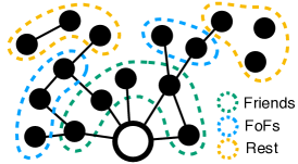
Figure 1. Illustration of a choice process in a small network. The ego chooses who to interact with, where different choice models may apply to friends, friends-of-friends, and others.

Discrete choice modeling provides a natural framework for modeling relational events (Butts, 2008; Stadtfeld and Block, 2017). Each event is viewed as a choice made by one node to involve another node, and modeled based on features of all the alternatives (see Figure 1). The conditional logit model of relational events subsumes and extends many existing models of network formation, such as preferential attachment and triadic closure (Overgoor et al., 2019). Yet in network analysis, the ability to work with large datasets is a major concern, where modeling relational events as choices raises both practical and conceptual issues.

The first set of issues pertains to the scale of the data. For a graph containing $n$ nodes, when the originator of the choice is known then every event represents a choice with $O(n)$ alternatives. For large and sparse graphs, the large slates of potential alternatives makes direct inference intractable. Existing frameworks for modeling network formation with a logit model, such as SAOMs (Snijders et al., 2010) and REMs (Butts, 2008), are severely restricted in the size of the data they can directly handle (Lerner and Lomi, 2020). Critically, however, under the conditional logit model the non-chosen alternatives can be sampled via a procedure commonly called “negative sampling” which produces estimates that are consistent for the estimates on the full data (McFadden, 1977; Train, 2009).

Availability, mixing, and de-mixing.  Another issue with applying the conditional logit model to large graph datasets is the availability assumption that the chooser is a rational actor who has complete information about their available options and their features. This assumption is obviously not realistic in large social networks, where nodes are generally not aware of the network at large and act mostly within their local social neighborhood. At the same time, in most social networks some edges happen outside the direct social neighborhood (Watts, 2003; Jackson and Rogers, 2007), which suggests the use of mixture models, mixing local and global processes (Kleinberg et al., 1999; Kumar et al., 2000; Jackson and Rogers, 2007). From a discrete choice viewpoint, these approaches specify mixed logit models (Overgoor et al., 2019).

The use of negative sampling does not cleanly transfer to the mixed logit setting (Guevara and Ben-Akiva, 2013). Part of our contribution is therefore to introduce a model simplification technique for discrete mixture models that we call “de-mixing” whereby the individual modes are forced to operate on disjoint sets. When the modes of a mixed logit model operate over disjoint choice sets, the resulting model reduces to a collection of individual conditional logit models. This de-mixing approach thus opens the door to negative sampling and high performance importance sampling-based approaches to negatives sampling, which we separately find to be an important underutilized tool for scaling discrete choice models. De-mixing also circumvents standard challenges with maximizing the likelihoods of mixture models, typically done via an EM algorithm (Train, 2009).

Importance sampling.  In practice, negative sampling is typically done uniformly, a procedure that can be very inefficient when important features are rare within the population. This inefficiency is particularly pronounced for modeling large-scale social networks, as they are frequently driven by activity within one’s local social neighborhood (Rapoport, 1953; Jin et al., 2001), which covers only a small subset of the full node set (making “is a friend of a friend” a rare feature). Furthermore, between 50% and 90% of new friendship edges form between existing friends-of-friends (Backstrom and Leskovec, 2011; Leskovec et al., 2008). Facebook’s People You May Know recommendation system was (as of 2013), built to only rank (and thus recommend) potential friends from existing friends of friends (Ugander and Backstrom, 2013). This concentration is even more pronounced for relational events, where pairs of individuals can interact repeatedly and often do. On the Venmo platform, which we analyze in this paper, approximately 73% of transactions in 2018 happened between people that had interacted before. In these settings, with the bulk of activity happening within the local neighborhood, uniform negative sampling is not a feasible solution.

To circumvent these issues and enable estimation of choice models on large graphs, we use importance sampling (Owen, 2013), a standard technique for approximate inference, to sample non-chosen alternatives non-uniformly. Importance sampling produces consistent estimates when coupled with an adjustment, based on the probability of being sampled, to the likelihood function. As a result, we can feasibly fit conditional logit models, both regular and de-mixed, that incorporate activity in the local neighborhood to very large graphs.

Applications.  We first illustrate the value of negative sampling on synthetic data with a known data generating process. We find that non-uniform importance sampling is especially effective for rare features that commonly drive network formation, where it can reduce the variance of the estimates by an order of magnitude. As an important inspection, we examine the trade-off between an overall downsampling of the data vs. sampling non-chosen alternatives within data points, and generally find that additional data points are more valuable (in terms of mean squared error) than additional negative samples. Model de-mixing, meanwhile, efficiently translates mixture models into conditional logit models, where negative sampling can be validly applied.

To illustrate the real-world feasibility of fitting discrete choice models to very large graphs, we introduce and analyze a large-scale dataset of public transactions on the Venmo platform. The data includes 501M public transactions, occurring between April 2012 and July 2018, involving 25M distinct user accounts. A single conditional logit model on this data results in extreme parameter estimates that are hard to interpret. However, a de-mixed mixed logit model shows that for local activity, well-known dynamics like reciprocity take place, while activity outside the local neighborhood appears to be primarily driven by preferential attachment. In this case, the de-mixed model provides significant new insight in the formation dynamics of this real world graph.

By de-mixing models that better approach the availability assumption and by leveraging non-uniform importance sampling, we find that discrete choice models can be scaled to large-scale relational event data with great potential for impact. These advances open up their use to diverse data mining applications, including but not limited to link prediction, anomaly detection, and general recommendation systems.

Additional related work.  Discrete choice models have a long history of study in psychology (Thurstone, 1927; Luce, 1959) and economics (McFadden, 1977; Agresti, 2003; Train, 2009). The conditional logit functional form has also been used to model network formation both more and less recently, including in exponential random graph models (ERGMs) (Robins et al., 2007), stochastic actor-oriented models (SAOMs) (Snijders et al., 2010), relational event models (REMs) (Butts, 2008), and dynamic network actor models (DyNAMs) (Stadtfeld and Block, 2017).

The concept of sampling non-chosen alternatives occurs in multiple literatures. In statistics and epidemiology, the technique is sometimes called case-control sampling (Langholz and Borgan, 1995). In econometrics, negative sampling is commonly used with conditional logit models (McFadden, 1977; Manski and McFadden, 1981; Agresti, 2003), while valid sampling for mixture models is an open problem (Nerella and Bhat, 2004; Guevara and Ben-Akiva, 2013; von Haefen and Domanski, 2018). Recent work explores sampling for models of network formation (Vu et al., 2015; Overgoor et al., 2019; Lerner and Lomi, 2020), but it is limited to uniform sampling for the conditional logit model. Our work expands to non-uniform sampling and provides a model simplification approach for mixture models.

In machine learning, negative sampling has found broad adoption for learning representations for text and graph mining (Mikolov et al., 2013; Tang et al., 2015), though in these contexts the way in which negative sampling changes the likelihood and the resulting representation output (due to model misspecification) is generally ignored. Thus it is important to emphasize that the change in the likelihood under misspecification has been of great concern to econometricians, where interpretable model parameters is a primary goal, whereas in representation learning the applied utility of the learned representations in downstream prediction tasks is most important, with interpreting the exact representations being of minimal interest.

Lastly, one prior study of Venmo transactions (Zhang et al., 2017) found dense clustering that frequently related to niche uses such as paying rent or settling betting pools. However, they do not model or analyze the factors driving the transactions.

2. Relational events as choices

Discrete choice models are commonly employed to model the factors driving a choice from a discrete slate of alternatives. Data points are individual choices $(i,j,C)$, indicating that agent $i$ chose item $j$ out of choice set $C$, where $C\subseteq U$ is typically a subset of some universe of alternatives $U$. The most popular class of discrete choice models is the random utility model (RUMs) (Manski and McFadden, 1981), where each alternative $j\in C$ can be thought of as providing some inherent utility to the agent $i$ making the choice, and the agent makes their choice by maximizing a noisy observation of that utility.

2.1. Conditional Logit

For the conditional logit model, the utility is modeled as a linear function of $x_{i,j}\in\mathbb{R}^{d}$, $j$’s features in the eyes of $i$, plus additive noise $\epsilon_{i}$:

$$U_{i,j}=\theta_{i}^{T}x_{i,j}+\epsilon_{i},$$

for some (latent) parameter vector $\theta_{i}\in\mathbb{R}^{d}$, which can be fixed or vary across individuals. Unless explicitly noted otherwise, we assume that the parameter vector $\theta$ is shared across individuals. When the noise terms are i.i.d. standard Gumbel, the probability of choosing each alternative is proportional to the exponentiated inherent utility $\theta^{T}x_{i,j}$ (Agresti, 2003):

(1) $$P_{i}(j,C)=\frac{\exp{\theta^{T}x_{i,j}}}{\sum_{\ell\in C}\exp{\theta^{T}x_{i,\ell}}}.$$

To see how this framework applies to relational events modeling, a relational event initiates a new edge $(i,j)$ in a directed network that can be seen as choice where node $i$ has chosen to connect or transact with node $j$, as opposed to any other node. The set of candidates for this choice, typically the full node set of the network at the time of the event, is then the choice set $C$. Our goal in fitting a discrete choice model to relational event data is to understand the potential role of different features $x_{i,j}$, which can be node covariates or information about the network structure at the time the edge was formed. As a concrete example, preferential attachment (Albert and Barabási, 1999) can be thought of as a conditional logit model with the single-element feature vector $x_{j,t}=\log d_{j,t}$, using only the candidate node $j$’s degree $d_{j,t}$ at time $t$. Many other network formation dynamics can easily be included in this modeling framework (Overgoor et al., 2019).

Conditional logit models with linear utility functions have a log-likelihood that is smooth and convex in the parameters $\theta$, meaning the maximum likelihood parameters can be efficiently estimated using, e.g., gradient descent or BFGS. The time complexity of fitting a conditional logit model with gradient descent with $n$ training examples and $s$ alternatives per example is then $O(ns)$ (Nesterov, 2013). This dependence of the time complexity on the different problem parameters is illustrated in Figure 2, where we plot the average runtime while varying $n$ and $s$. While the runtime is linear in $ns$, different choices of $n$ and $s$ at constant $ns$ can have different bias and accuracy, as we explore in Section 4.1.

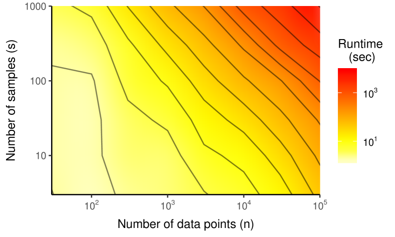
Figure 2. The runtime (in seconds) of training a conditional logit model, varying the number of choices $n$ and number of alternatives to choose from $s$, is roughly linear in both dimensions. Each point represents the average of 50 runs.

2.2. Heterogeneity with known context

The conditional logit, as presented so far, assumes a single parsimonious parameter vector $\theta$ that is shared across all agents and in all contexts, while it’s clear that preferences may vary over both agents and contexts. First, different kinds of choosers can have differing preferences. For example, men and women may have different styles of making friendships, as may students and non-students (Currarini et al., 2010). In the limit, individuals can have their own personal preference, though this can only be modeled when one has considerable data for each individual. On the other hand, the choice context could affect preferences. For example, people make different decisions at different stages in their careers, and their choices can depend on their moods or the choice interface (Chen and Joachims, 2016; Seshadri et al., 2019).

If the chooser type or choice context is known, it is relatively straightforward to model heterogenous preferences. The analyst can fit separate parameters $\theta_{i}$ for each “group” $i$, or, if some parameters are hypothesized to be shared across groups, interact the context and the context-dependent features. Because the conditional logit estimates the relative utility of items within a choice set, one cannot simply include the choice context as an interaction term, as one would do with a regression model. Instead, the interaction can be implemented by one-hot coding each coefficient for each context, and setting the value to 0 when the context feature does not apply (Agresti, 2003). This conveniently avoids co-linearity and keep the model identifiable, provided that there are enough data points for each context-feature value combination.

2.3. Mixed Logit for latent context

When the choice context is unknown, one can still model heterogeneous choice using a mixed logit approach with latent variables. In general, a mixed logit model is defined using a continuous probability distribution $f$ over different instances of the parameters $\theta$. In this work, we will only consider discrete mixtures of $M$ different parameters (called “modes”), an approach also called a latent class model. The choice probability is then:

(2) $$P_{i}(j,C)=\sum_{m=1}^{M}\pi_{m}\frac{\exp{\theta^{T}_{m}x_{j}}}{\sum_{\ell\in C_{m}}\exp{\theta^{T}_{m}x_{\ell}}}\mathbf{1}[j\in C_{m}],$$

where the class weights $\pi_{m}\geq 0$ model the relative prevalence of each mode and $\sum_{m=1}^{M}\pi_{m}=1$. Each mode thus has its own preference vector $\theta_{m}$ and can have its own limited choice set $C_{m}$ as long as $C_{m}\subseteq C$. Maximizing the likelihood of a mixed logit model is harder than for the conditional logit, since the log-likelihood is not convex in general. A common solution is to use expectation maximization (EM) (Train, 2009). However, EM can be slow to find even a locally optimal solution, since there often is a trade-off between changing the class weights and changing the feature weights.

A mixed logit model greatly increases the degrees of freedom the analyst has to fit a model to their data. There can be many options for how to specify the choice set $C_{m}$ of each mode, which could be identical, disjoint, or exhibit arbitrary overlap. Care should be taken with formulating a hypothesis on how the data was generated, and to use model selection and robustness checks while doing inference.

2.4. Mixed logit and de-mixing

In modeling relational events, the mixed logit formulation subsumes a number of popular network formation models such as the copy model (Kleinberg et al., 1999; Kumar et al., 2000) and the local search model (Jackson and Rogers, 2007; Holme and Saramäki, 2012). The local search model attempts to address the availability assumption, discussed in the introduction, by mixing two modes where the first mode is restricted to a choice set of friends-of-friends of the chooser $i$, which we denote as $FoF_{i}$, while the second mode makes unrestricted choices from the full node set $V$. The standard local search model assumes very simple utility functions for each of the two modes, letting the difference in choice sets do most of the heavy lifting. Typically the utility function on the unrestricted choice set is constant, meaning that it can really be viewed as a “garbage collection” mode, capturing rare friendship events to non-friends-of-friends without any attempt to model specific mechanisms of such events. The local search model is thus an attractive approach to addressing the availability assumption, but introduces all of the above disadvantages of mixed logits. However, in any realistic social network, it’s clear that the sets $FoF_{i}$, for all $i$, will generally be very small subsets of the full node set. This observation motivates the de-mixing approach that we now introduce.

What makes fitting a standard mixed logit model hard is that when a chosen alternative is available in the choice sets $C_{m}$ of several modes, a given data point can have very similar conditional likelihoods under different modes. However, when the chosen alternative is only available in the choice set of a single mode, the choice uniquely identifies the mode, collapsing the mixture. Thus, when the choice sets of the modes are fully disjoint, every data point $j$ has a non-zero likelihood only for the mode $m$ where $j\in C_{m}$. Phrased in the language of Sections 2.2 and 2.3, it is as if the choice context is known. We call this approach, whereby a mixture model with nearly disjoint choice sets is approximated by a model with forcibly disjoint choice sets, “de-mixing”.

What does de-mixing give us? When estimating a disjoint mixed logit, the class parameters $\pi_{m}$ then follow directly from the data and the preference parameters $\theta_{m}$ can be found by fitting $m$ individual conditional logit models. To illustrate, the log-likelihood of the model on disjoint choice sets $C_{m}$ fit to the full data can be written:

$$\begin{split}l(\theta;\mathcal{D})&=\log\prod_{(j,C)\in\mathcal{D}}\sum_{m}^{M}\pi_{m}\frac{\exp{\theta^{T}_{m}x_{j}}}{\sum_{l\in C_{m}}\exp{\theta^{T}_{m}x_{l}}}\mathbf{1}[j\in C_{m}]\\ &=\sum_{m}^{M}\log\prod_{(j,C)\in\mathcal{D}_{m}}\frac{\exp{\theta^{T}_{m}x_{j}}}{\sum_{l\in C_{m}}\exp{\theta^{T}_{m}x_{l}}}=\sum_{m}^{M}l(\theta_{m},\mathcal{D}_{m}),\ \end{split}$$

where $\mathcal{D}_{m}=\{(j,C)\in\mathcal{D}\ :\ j\in C_{m}\}$ are the disjoint subset of the data where the choice was made from the mode’s reduced choice set. The mode-level features $\theta_{m}$ can thus be estimated separately, even in parallel, on the different disjoint subsets of the data.

Given the greatly simplified likelihood, mixture models with disjoint choice sets are highly attractive. As we will see in Section 3, the return to conditional logits re-introduces the validity of negative sampling, at least under the model class, which is essential for scalable inference. Depending on the analysis context, de-mixing may thus constitute a minor simplification with great practical implications. For example, in the local search model discussed above, the choice sets $C_{1}=FoF_{i}$ and $C_{2}=V$ are often very nearly disjoint. By slightly modifying the second choice set to be $C_{2}=V\setminus FoF_{i}$, we get a model that is easy to estimate on very large graphs.

3. Sampling of alternatives

In large real-world graphs, the choice set $C$ of alternatives (all nodes) quickly become prohibitively large. To make estimating a conditional logit model computationally tractable in such settings, one can estimate the same model on reduced choice sets of alternatives. Specifically, $s-1$ negative/non-chosen examples can be sampled to create a (random) reduced dataset with smaller choice sets. For each choice $(j,C)$, one forms a smaller random choice set out of the positive choice and the negative samples, $\tilde{C}\subset C$ with $\lvert\tilde{C}\rvert=s$, and replaces the original choice data with $(j,\tilde{C})$.

McFadden showed that asymptotically (in the limit of large datasets), estimates on a data set with reduced choice sets generated with importance sampling are consistent (in the limit of many data points) for the estimates using complete choice sets, provided that the true process is within the model class of conditional logit (McFadden, 1977, eq. 40-41). Phrased another way, this classic econometric result highlights that estimation under negative sampling does not offer a consistency guarantee outside the model class. As a result, outside the model class it is clear that different sampling distributions and different negative sample budgets $s$ can lead to very different parameter estimates.

Within the correct model class, to produce estimates that are consistent one has to adjust the likelihood function. Individual examples need to be weighted based on the sampling probability of the reduced choice set $\tilde{C}$.

Following (McFadden, 1977; Ben-Akiva et al., 1985), for a reduced choice set $\tilde{C}\subseteq C$ the choice probability is then

(3) $$P_{i}(j,\tilde{C})=\frac{\exp{\big{(}\theta^{T}x_{j}-\log q_{j}}\big{)}}{\sum_{\ell\in\tilde{C}}\exp{\big{(}\theta^{T}x_{\ell}-\log q_{\ell}\big{)}}},$$

where $q_{x}$ is the probability, under the importance sampling distribution, of including element $x$ in the reduced choice set $\tilde{C}$ independently from other alternatives.

Uniform sampling.  The most straightforward sampling procedure is uniform sampling, which makes every individual alternative equally likely to be chosen. Under uniform sampling (without replacement), the probabilities $q_{x}$ are all equal and cancel out. Therefore, no adjustments is necessary to have consistent parameter estimates under uniform sampling.

Stratified sampling.  Uniform negative sampling ignores both the relative frequency and the relative importance of features in the data, and is therefore not an efficient way to estimate the parameters. Stratified sampling can be used to create choice sets that are balanced with respect to one or more categorical dimensions. As a relevant example, we can construct strata for friends, friends-of-friends, and other nodes (recall Figure 1). Practically, a pre-specified amount of alternatives is sampled for each specific stratum $G$ (uniformly at random within the stratum). The sampling weights are proportional to the relative sizes of the categories within the full choice sets. When sampling $s$ alternatives for a specific stratum $G$, of which there are $n_{G}$ elements in the full choice set ($n_{G}=|G\cap C|$), the sampling weight for an individual item $x$ becomes $q_{x}=\frac{s}{n_{G}}$. Now, Equation (3) can be used to produce consistent estimates of the parameters. This approach is flexible with respect to the way strata are defined. For example, multiple dimensions can be crossed and continuous features can be bucketed.

Importance sampling.  Stratified sampling is a special case of importance sampling. An importance sampling policy assigns to each element $x$ its own sampling probability $q_{x}$ (Owen, 2013, Ch. 9). The estimator is consistent regardless of the choice of the importance sampling weights, but better weights can reduce the variance of the estimator. More efficient than having balanced strata is to sample elements of $\tilde{C}$ proportional to the likelihood of being chosen. In the optimal sampling policy, the relative likelihood of choosing the positive and negative samples should vary as little as possible (Ben-Akiva et al., 1985, page 264). However, in order to compute these choice probabilities, this hypothetical optimal policy presumes the availability of the very feature weights that we are trying to estimate. For example, if the actual true feature weight for some binary covariate is $\beta$, then the ideal rate between the sampling probabilities for options with and without that covariate is $\exp(\beta)$.

There are various ways in which proxies for the importance sampling probabilities can be obtained, including employing domain knowledge, using a parametric model to obtain sampling weights for a non-parametric model, sequentially fitting a crude model and then a finer model, and/or to compute unweighted empirical choice probabilities from the data. We leave exploration of these diverse approaches for future work, focusing on the high relevance of stratified sampling based on friends and friends-of-friends.

Sampling for Mixed Logit.  For the general class of mixed logit models, estimates on a (negatively sampled) reduced choice set are not consistent for the estimates on the full choice set (Guevara and Ben-Akiva, 2013). To correct the bias, the likelihood has to be adjusted with factors $W^{1}_{n},\ldots,W^{M}_{n}$ representing the likelihood of sampling the reduced choice set $\tilde{C}$ when $j$ is chosen for each of the $M$ modes. Unfortunately, the quantity $W_{n}^{m}$ is not easily computed, as it relies on the choice probability of the full choice set(!), rather than the reduced choice set $\tilde{C}$. Various heuristic approaches have been proposed to attempt uniform negative sampling (Nerella and Bhat, 2004; von Haefen and Domanski, 2018; Guevara and Ben-Akiva, 2013). While empirical results have generally been promising, a full evaluation of these specific approaches has to be left for future work. The lack of guarantees for fitting mixed logit models on negatively sampled data strongly limits their utility for most realistic network data sets. In the de-mixed logit setting, however, the sampling techniques of the conditional logit can be applied to each mode individually.

4. Applications on Synthetic data

In this section we illustrate the benefits and applications of sampling non-chosen alternatives for conditional logit models on relational event data. In the first example we explore the benefits for inference from importance sampling on a data set with a known data generating process. The next example studies how negative sampling can alter the estimates when the model is misspecified. Applications to real-world data follow in Section 5. For the reproducibility of our results, we’ve shared the code for these synthetic experiments at https://github.com/janovergoor/choose2grow/.

4.1. Synthetic conditional logit experiments

If choice sets are small, it is computationally feasible to consider all non-chosen alternatives when maximizing the likelihood, which will lead to the best parameter estimates given the data. With relational data, however, the choice sets are typically enormous, necessitating sampling. Importance sampling is motivated by item features that are unequally distributed in the choice set. The advantage over uniform sampling is especially pronounced when the number of data points is small, or when it is not feasible to consider many non-chosen alternatives. To illustrate this advantage, we construct a synthetic data example showing the benefits of stratified sampling, a simple form of importance sampling.

Data generation.  We simulate events happening between members of a fixed population of $N$=5,000 nodes. To seed a graph, we generate $|E|$=25,000 events by uniformly sampling the nodes $(i,j)$. We then sequentially generate 160,000 events (data points) where for each event we first sample the “sending node” $i$ uniformly at random. Every possible “target node” $j$ for the event then has a utility based on a pre-specified utility function with four principle features taken in two transformations (thus, eight features): $j$’s in-degree (representing popularity), number of prior events from $i$ to $j$ (representing repetition), number of prior events from $j$ to $i$ (representing reciprocity), and the number of unique friends of friends between $i$ and $j$. For these four principle features we apply two transformations: we take the log (mapping $\log 0$ to $0$), as well as an indicator feature for whether the value is non-zero. We set the parameter values to $(0.5,2,2,2)$ for the log features, and $(1,4,4,4)$ for the indicator features.

Varying $n$.  We construct data sets of incrementally increasing size (so that the smaller data set is contained in the larger data sets), and for each total of $n$ data points, we consider $s-1$ negative samples for $s=24$ under both uniform and stratified sampling. For stratified sampling, $s/3$ negative samples are taken from each of three groups: friends (have interacted with before), friends-of-friends (friends have interacted with before), and the rest. For every incremental dataset, we fit a conditional logit model with the same specification as the utility function we used to generate the data.

Figure 3. Top row: The range of estimates (left) and MSE of the point estimates (right) for the reciprocate feature (true value $\theta_{\text{rec}}$=2) when varying $n$. Bars represent 5/95 and 25/75 inter-quantile ranges of 100 estimates. Importance sampling has an MSE that’s an order of magnitude smaller than uniform sampling. Bottom row: the range of MSEs, when varying $s$, keeping $n$ constant at $n$=10,000 (left) and with a fixed budged for $ns$=480,000 (right). Importance sampling achieves high-precision estimates even for low values of $s$. With a fixed budget on $ns$, MSE is lowest for small $s$.

We focus our discussion on one representative feature, reciprocity, as an example of a feature that benefits from oversampling from the immediate social neighborhood. In Figure 3 we plot the ranges of the estimates (top-left) and mean squared error of the estimates (top-right). As expected, the error decreases as the number of data points increases for both negative sampling methods. Also, as $n$ increases, the MLE converges to the true value of $\theta_{\text{rec}}$=2. For low values of $n$ and $s$, there are simply not enough examples of non-chosen alternatives that can be reciprocated with, so non-uniform sampling is much more effective. The improvement in the error from using stratified sampling (over uniform sampling) is approximately an order of magnitude at these values of $n$. The other features that are also related to the chooser’s social neighborhood similarly benefit from stratified sampling (not shown). The benefit of importance sampling is most pronounced for features that are unequally distributed in the data of alternatives.

Varying $s$.  Next, we fit the same model, but keep the number of training examples constant at $n$=10,000 and vary $s$. The range of mean squared errors for the reciprocity parameter are again shown in the bottom-left panel of Figure 3. Uniform negative sampling benefits from increases in $s$. Importance sampling achieves high-precision estimates even for low values of $s$, because each data points has a minimum number of high-utility alternatives. For higher value of $s$, importance sampling achieves the same MSE as the estimate of the full choice set without negative sampling.

Varying $n$ and $s$ under a budget.  Increasing $s$ improves the estimates for uniform sampling, but doing so linearly increases the volume of the training data and the runtime of the optimization procedure, as indicated by the discussion of time-complexity in Section 2.1. Therefore, paralleling an analysis of SAOM (Snijders et al., 2010) in (Lerner and Lomi, 2020), we ask whether increasing $n$ or $s$ is preferred at a given runtime budget. We study a fixed budget of $ns$=480,000, so that as we increase $s$, we decrease $n$. We display the resulting estimates for $\theta_{\text{rec}}$ in the bottom-right panel of Figure 3. For both uniform and non-uniform sampling, smaller $s$ perform better. However, for uniform sampling this effect is small as the MSE is relatively uniform. Meanwhile, for stratified sampling we observe significantly more precise estimates at lower values of $s$, up until $s=24$. We emphasize that this specific inflection point ($s=24,n=20,000$) does not provide a general recommendation for practitioners about how to optimally trade off $n$ and $s$, but rather, we provide this analysis as a demonstration that practitioners should actively consider this trade-off when training choice models of relational data.

4.2. Model misspecification

As mentioned in the introduction, McFadden’s celebrated result on consistency under negative sampling assumes that the data was generated from the correct model class. In this section, we examine negative sampling when used outside the model class.

Data generation.  We use a similar data generation process as in Section 4.1. We generate a single event graph with $N=$5,000 nodes and seed it with uniformly sampled pre-events. We then generate 80,000 choices from a 2-mode mixed logit with disjoint choice sets (a de-mixed model). The first (“local”) mode considers only friends and friends-of-friends, and has the feature vector $\theta=(0.5,1,1,1,0.5,1,1,1)$. Each mode has the same eight feature as in Section 4.1. The second mode considers all other nodes (recall it is a de-mixed model), and has the feature vector $\theta=(1,0,0,0,1,0,0,0)$, which effectively gives utility only to degree. The local mode has weight $\pi=0.75$ in the mixture model.

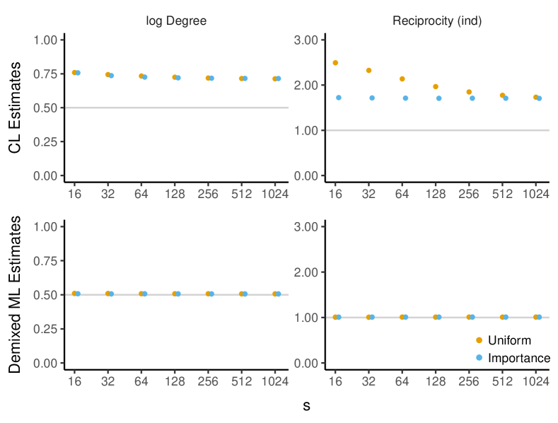
Figure 4. Estimates for the log degree (left) and reciprocate (right) features under 2-mode mixed-logit data, fit with a conditional logit model (top) and a mixed-logit model with a local neighborhood mode (bottom). Bars (not visible) represent 5/95 and 25/75 inter-quantile ranges of 100 estimates. The misspecified CL estimates vary as a function of $s$ and the sampling methods. The correctly specified ML estimates are well-behaved when negatively sampled.

Fitting a misspecified conditional logit.  First, we fit a single conditional logit model to this data, with correctly specified features but only as a single mode instead of two. The resulting estimates under different values of $s$ are shown in Figure 4 (top row). We focus on two features: log degree and the indicator function for reciprocity. The range of estimates for both features is practically in-between the true values of the parameter for the two modes (0.5 and 1 for log degree and 4 and 0 for reciprocity). Worse, the estimates are not stable across different values of $s$. Uniform sampling especially gives very different estimates for low values of $s$. Only when $s$ approaches the full choice set do the two different sampling methods agree. Caution should always be taken when fitting a conditional logit with negative sampling, and it is important to verify that different meta-decisions (such as $n$, $s$, and the sampling policy) give stable estimates. If not, this stability analysis can be a diagnostic signal that the data was generated outside the model class.

De-mixed model fit.  Next, we fit the correctly specified model class to the data: a mixed logit with disjoint choice sets. In practice, this amounts to separating the data points into the different modes based on the features of the chosen example, and fitting a conditional logit to the alternatives from the same mode. The class probability $\pi_{m}$ follow directly from the data, in this case $\hat{\pi}_{1}=0.743$. In Figure 4 (bottom row), we present the estimates for the “local” mode. The estimates are highly accurate. Also, the two sampling policies gives relatively stable estimates under different values of $s$. This is not surprising, as the de-mixed modeling approach places the model within the conditional logit model class.

5. Empirical analysis of Venmo Data

Venmo is a mobile payment platform that supports person-to-person financial transactions. Since 2012 Venmo has seen a rapid growth in its transaction volume, both through growth in its active user base and in payments per user. As compared to other mobile transaction platforms, Venmo usage occurs more within social groups (Zhang et al., 2017). Therefore, the structure of the Venmo payment network is likely correlated with the structure of the social interactions of its users, and may exhibit similar structural phenomena.

The Venmo graph records transactions that can occur multiple times between the same two people, similar to instant messaging networks (Leskovec and Horvitz, 2008). As of July 2018, Venmo published all of its public transactions through their API, which allowed anyone to request all the public transactions that occurred within a specified timeframe. Transactions up until that point were public by default if both of the accounts have their privacy settings set to “public by default”.

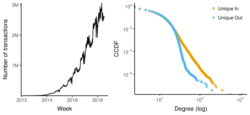
Figure 5. The number of transactions per week (left) and the complementary cumulative degree distribution (right) of the Venmo transaction dataset. Degree is counted as the number of unique transaction alters.

We retrieved all public transactions between April 12, 2012 and July 17, 2018, collected under an IRB-approved research protocol. The data includes 25M users, out of a total of 39M (derived from the incremental user IDs). The transaction IDs imply that there were 501M public transactions out of a total of approximately 1B transactions. Among the transacting actors are individual user accounts as well as companies and organizations identifiable through their user name. Venmo grew considerably during the time span of the dataset, and we can see that the number of users and transactions grow in shown in Figure 5 (left), where it is also easy to see seasonal effects. The overall degree distribution, computed as the number of unique accounts transacted with, is shown in Figure 5 (right). There are not so many accounts sending large amounts of transactions, with the cash-back company Ibotta as a single previously-documented exception (Zhang et al., 2017). Transactions primarily re-occur within a local social neighborhood: in 2018, 73% of transactions happened between people that had transacted previously and another 6.8% happened between friends-of-friends.

5.1. Model-based analysis

To understand the dynamics in the transaction data, we fit both a conditional logit and a de-mixed mixed logit model to the Venmo data. Following standard practice in relational event modeling (Butts, 2008; Lerner and Lomi, 2020), we construct the following features from the event data:

• $|F_{j}|$ – the number of unique nodes interacting with node $j$,

• $\#_{\rightarrow j}$ – the times $j$ received money, proxy for $j$’s popularity,

• $\#_{i\rightarrow j}$ – the times $i$ sent $j$ money before, proxy for repetition,

• $T_{\rightarrow j}$ – the time since $j$ received money (in seconds),

• $T_{j\rightarrow}$ – the time since $j$ sent money,

• $T_{i\rightarrow j}$ – the time since $i$ sent $j$ money, proxy for repetition,

• $T_{j\rightarrow i}$ – the time since $j$ sent $i$ money, proxy for reciprocity,

• $|FoF_{ij}|$ – the number of unique nodes forming length-2 forward paths from $i$ to $j$.

Each temporal feature is transformed with $\log T^{-1}$ and each counting measure is log-transformed (where $\log 0=0$) and has an indicator feature (indicating if that the value is non-zero). We include the time feature to focus on recency, rather than volume. However, we do keep an indicator function for $j$ receiving any message and $j$ receiving a message from $i$.

We sampled 1% the public Venmo transactions between 2018-06-26 and 2018-07-17 for analysis. We fit both a conditional logit model and a de-mixed mixed logit model to illustrate their differences. For the conditional logit model, we constructed the data using stratified negative sampling, with strata for friends, friends-of-friends, and the rest ($100$ nodes/stratum). For the mixed logit model, there are two modes that can be estimated separately. The first “local” mode considers only friends and friends-of-friends of the choosing node as possible candidates. Since friends are still much more likely to be chosen than friends-of-friends, we also apply stratified negative sampling with two strata for friends and friends-of-friends ($100$ nodes/stratum here). The second “rest” mode considers all other nodes as possible candidates. Negative examples for this mode are sampled uniformly.

5.2. Results

The resulting parameter estimates are displayed in Table 1. For each coefficient, the standard errors are also provided.

Conditional logit.  The estimates for the conditional logit model are dominated by the indicator feature for $i$ having transacted with $j$ before. The parameter estimate of 13.443 would imply a factor of 689,000x ($\approx\exp 13.443$) more likely to be chosen. This value is directly related to the relative size of the non-local node set, and thus hard to interpret. The number of friends-of-friends is also a strong factor related to the local neighborhood. For the rest, the recency of $j$ receiving any money if a major factor. The positive estimate for the feature representing the time since a transaction from $j$ to $i$ is soft evidence for a version of reciprocity. Net of these other features, the negative coefficient for $\log|F_{j}|$ is consistent with negative “preferential attachment” (Albert and Barabási, 1999).

De-mixed mixed logit.  Because the modes of the de-mixed mixed logit are defined over disjoint choice sets, the class probability estimates follow directly from counts of the data. For this month of data, 82.9% of transactions happened within the local neighborhood. A major difference compared to a single-mode model is that the coefficient for popularity “split” into a negative component for local ties and a positive component for non-local ties. When a node is already known, its popularity is less important. But when it is not known, popularity is a major predictor of connecting. The other coefficients show minor differences with respect to the single-mode model. The coefficient for “is friend” is still very strong in the local mode, but orders of magnitude less so. Reciprocity is strong, with both $j$ sending and $j$ sending to $i$ being important features.

Non-parametric estimates.  To further illustrate the difference between the two modes, we fit another de-mixed mixed logit model with the in-degree (number of transactions) as a (non-parametric) feature, so there is just an indicator feature for every individual in-degree. We plot the estimated relative probabilities of choosing a node $j$ with degree $k_{j}$, as compared to choosing a node with degree 1, in Figure 6. As in the full model results, in-degree matters less for nodes in local neighborhoods than it does for nodes that are further out. For nodes outside the neighborhood, the in-degree has a super-linear relationship with utility. These high-degree nodes probably represent small businesses or organizations that receive incoming transactions from many different actors (Zhang et al., 2017).

Table 1. Logit model fits for Venmo transaction data. The conditional logit model is estimated using stratified negative sampling. The mixed logit model has two modes with disjoint choice sets: one for local nodes (friends and friends-of-friends) and one for the rest.

	Conditional	Mixed Logit
	Logit	Local	Rest
log $|F_{j}|$	-0.032* (0.001)	-0.377* (0.001)	0.573* (0.002)
log $T^{-1}_{\rightarrow j}$	-0.192* (0.002)	0.357* (0.000)	0.413* (0.001)
log $T^{-1}_{j\rightarrow}$	0.381* (0.000)	-0.015* (0.000)	-0.056* (0.001)
log $T^{-1}_{i\rightarrow j}$	-0.002* (0.000)	0.085* (0.001)
log $T^{-1}_{j\rightarrow i}$	0.102* (0.000)	0.375* (0.000)
log $|FoF_{ij}|$	0.390* (0.000)	0.451* (0.002)
$\mathbbm{1}[\#_{\rightarrow j}>0]$	-0.422* (0.005)	-1.115* (0.008)	-1.290* (0.007)
$\mathbbm{1}[|F_{j}|>0]$	-0.624* (0.006)	0.000* (0.032)	-1.898* (0.007)
$\mathbbm{1}[\#_{i\rightarrow j}>0]$	13.443* (0.003)	3.008* (0.003)
$\mathbbm{1}[|FoF_{ij}|>0]$	1.046* (0.002)	0.336* (0.002)
$\pi_{m}$		0.829	0.171
Observations	129,098	106,540	21,973
Note:	*p$<$0.01

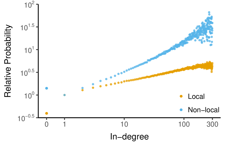
Figure 6. Non-parametric estimates of the relative value (compared to degree 1) of in-degree for receiving a transaction on Venmo. Degree matters less for nodes in the local neighborhood and is valued super-linearly for other nodes.

6. Discussion

Understanding the factors driving choice behavior has many applications in the study of social networks and other relational data. Discrete choice models provide a principled way to model the multiple factors driving these decisions. Model-based analysis allows one to analyze, for example, how a platform change affects user behavior in a randomized experiment. Having a more detailed model of behavior also enables anomaly detection by identifying unlikely behaviors or sequences of behaviors. In this work, we have proposed methods to fit choice models to large-scale relational event data. De-mixing decomposes the mixed logit into multiple conditional logit models that are easy to estimate. Importance sampling allows for the estimation of rare features. Both methods fit well with the insight that most activity in social networks is inherently local.

We briefly point to several open research questions. First, a more formal theory of when it is better to increase the number of data points $n$ or the number of choice alternatives $s$ is needed (“to sample or to negatively sample?”). Decisions along this tradeoff likely depend on the model class, distribution of the features, and the variance of the “true” covariates. We also note the need to further work out how varied choice models, e.g. the nested logit model or context-dependent utility model (Seshadri et al., 2019), can be employed for modeling network formation, and how negative sampling works for those models.

Even though the de-mixed mixed logit model has many applications, many other applications require the ability to consider overlapping choice sets. For example, in some applications, different transaction types can apply to overlapping sets of targets. For these applications to be practically feasible, it is important to be able to fit mixed logit models on reduced choice data. Further studies of the sampling adjustment for the mixed logit would be welcome. Finally, there is potential work in finding bridges between choice models and other data mining applications such as sequence embedding models and recommender systems.

Acknowledgements.  We thank Austin Benson, Lodewijk Gelauff, Jürgen Lerner, John Levi Martin, and Arjun Seshadri for helpful comments and discussions. This work is funded in part by support from the Stanford Thailand Research Consortium and a Young Investigator Award from the Army Research Office (73348-NS-YIP). Data collection approved under Stanford protocol IRB-46422.

References

- (1)
- Agrawal et al. (1993) Rakesh Agrawal, Tomasz Imieliński, and Arun Swami. 1993. Mining association rules between sets of items in large databases. In ICMD. ACM, 207–216.
- Agresti (2003) Alan Agresti. 2003. Categorical data analysis. Vol. 482. John Wiley & Sons.
- Akoglu et al. (2015) Leman Akoglu, Hanghang Tong, and Danai Koutra. 2015. Graph based anomaly detection and description: a survey. Data mining and knowledge discovery 29, 3, 626–688.
- Albert and Barabási (1999) Réka Albert and Albert-László Barabási. 1999. Emergence of scaling in random networks. Science 286, 5439, 509–512.
- Backstrom and Leskovec (2011) Lars Backstrom and Jure Leskovec. 2011. Supervised random walks: predicting and recommending links in social networks. In WSDM. ACM, 635–644.
- Ben-Akiva et al. (1985) Moshe E Ben-Akiva, Steven R Lerman, and Steven R Lerman. 1985. Discrete choice analysis: theory and application to travel demand. Vol. 9. MIT press.
- Benson et al. (2018a) Austin R Benson, Rediet Abebe, Michael T Schaub, Ali Jadbabaie, and Jon Kleinberg. 2018a. Simplicial closure and higher-order link prediction. PNAS 115, 48, E11221–E11230.
- Benson et al. (2018b) Austin R Benson, Ravi Kumar, and Andrew Tomkins. 2018b. A Discrete Choice Model for Subset Selection. In WSDM. ACM, 37–45.
- Bruch and Mare (2012) Elizabeth E Bruch and Robert D Mare. 2012. Methodological issues in the analysis of residential preferences, residential mobility, and neighborhood change. Sociological methodology 42, 1, 103–154.
- Butts (2008) Carter T Butts. 2008. A Relational Event Framework for Social Action. Sociological Methodology 38, 1, 155–200.
- Chen and Joachims (2016) Shuo Chen and Thorsten Joachims. 2016. Predicting matchups and preferences in context. In KDD. ACM, 775–784.
- Currarini et al. (2010) Sergio Currarini, Matthew O Jackson, and Paolo Pin. 2010. Identifying the roles of race-based choice and chance in high school friendship network formation. PNAS 107, 11, 4857–4861.
- Ghasemian et al. (2019) Amir Ghasemian, Homa Hosseinmardi, Aram Galstyan, Edoardo M Airoldi, and Aaron Clauset. 2019. Stacking Models for Nearly Optimal Link Prediction in Complex Networks. arXiv preprint arXiv:1909.07578.
- Guevara and Ben-Akiva (2013) C Angelo Guevara and Moshe E Ben-Akiva. 2013. Sampling of alternatives in Logit Mixture models. Transportation Research Part B 58, C, 185–198.
- Holme and Saramäki (2012) Petter Holme and Jari Saramäki. 2012. Temporal networks. Physics Reports 519, 3, 97–125.
- Jackson and Rogers (2007) Matthew O Jackson and Brian W Rogers. 2007. Meeting Strangers and Friends of Friends: How Random Are Social Networks? AER 97, 3, 890–915.
- Jarvis (2018) Benjamin F Jarvis. 2018. Estimating Multinomial Logit Models with Samples of Alternatives. Sociological Methodology 49, 1, 341–348.
- Jin et al. (2001) Emily M Jin, Michelle Girvan, and Mark EJ Newman. 2001. Structure of growing social networks. Physical Review E 64, 4, 046132.
- Kleinberg et al. (1999) Jon M Kleinberg, Ravi Kumar, Prabhakar Raghavan, Sridhar Rajagopalan, and Andrew S Tomkins. 1999. The web as a graph: measurements, models, and methods. In ICCC. Springer, 1–17.
- Kossinets and Watts (2006) Gueorgi Kossinets and Duncan J Watts. 2006. Empirical analysis of an evolving social network. Science 311, 5757, 88–90.
- Kumar et al. (2000) Ravi Kumar, Prabhakar Raghavan, Sridhar Rajagopalan, D Sivakumar, Andrew Tomkins, and Eli Upfal. 2000. Stochastic models for the web graph. In Proceedings of the 42st Annual Symposium on Foundations of Computer Science. IEEE, 57–65.
- Langholz and Borgan (1995) B Langholz and Ørnulf Borgan. 1995. Counter-matching: a stratified nested case-control sampling method. Biometrika 82, 1, 69–79.
- Lerner and Lomi (2020) Jürgen Lerner and Alessandro Lomi. 2020. Reliability of relational event model estimates under sampling: how to fit a relational event model to 360 million dyadic events. Network Science 8, 1, 97–135.
- Leskovec et al. (2008) Jure Leskovec, Lars Backstrom, Ravi Kumar, and Andrew Tomkins. 2008. Microscopic evolution of social networks. In KDD. ACM, 462–470.
- Leskovec and Horvitz (2008) Jure Leskovec and Eric Horvitz. 2008. Planetary-scale views on a large instant-messaging network. In WWW. ACM, 915–924.
- Liben-Nowell and Kleinberg (2007) David Liben-Nowell and Jon Kleinberg. 2007. The link-prediction problem for social networks. Journal of the American society for information science and technology 58, 7, 1019–1031.
- Luce (1959) R Duncan Luce. 1959. Individual Choice Behavior; a Theoretical Analysis. New York, Wiley.
- Manski and McFadden (1981) C F Manski and Daniel McFadden. 1981. Alternative estimators and sample designs for discrete choice analysis. In Structural Analysis of Discrete Data and Econometric Applications. 2–50.
- McFadden (1977) Daniel McFadden. 1977. Modelling the Choice of Residential Location. Cowles Foundation Discussion Papers 477. Yale University.
- McPherson et al. (2001) Miller McPherson, Lynn Smith-Lovin, and James M Cook. 2001. Birds of a feather: Homophily in social networks. Annual Review of Sociology 32, 1, 19–28.
- Mikolov et al. (2013) Tomas Mikolov, Ilya Sutskever, Kai Chen, Greg S Corrado, and Jeff Dean. 2013. Distributed representations of words and phrases and their compositionality. In NeurIPS. Curran Associates, 3111–3119.
- Nerella and Bhat (2004) S Nerella and C Bhat. 2004. Numerical analysis of effect of sampling of alternatives in discrete choice models. J of Transportation Research 1894, 1, 11–19.
- Nesterov (2013) Yurii Nesterov. 2013. Introductory lectures on convex optimization: A basic course. Vol. 87. Springer Science & Business Media.
- Noble and Cook (2003) Caleb C Noble and Diane J Cook. 2003. Graph-based anomaly detection. In KDD. ACM, 631–636.
- Overgoor et al. (2019) Jan Overgoor, Austin Benson, and Johan Ugander. 2019. Choosing to Grow a Graph: Modeling Network Formation As Discrete Choice. In WWW. ACM, 1409–1420.
- Owen (2013) Art B. Owen. 2013. Monte Carlo theory, methods and examples.
- Rapoport (1953) Anatol Rapoport. 1953. Spread of information through a population with socio-structural bias: I. Assumption of transitivity. The bulletin of mathematical biophysics 15, 4, 523–533.
- Robins et al. (2007) Garry Robins, Pip Pattison, Yuval Kalish, and Dean Lusher. 2007. An introduction to exponential random graph (p*) models for social networks. Social networks 29, 2, 173–191.
- Seshadri et al. (2019) Arjun Seshadri, Alex Peysakhovich, and Johan Ugander. 2019. Discovering Context Effects from Raw Choice Data. In ICML. PMLR, 5660–5669.
- Snijders et al. (2010) Tom AB Snijders, Gerhard G Van de Bunt, and Christian EG Steglich. 2010. Introduction to stochastic actor-based models for network dynamics. Social networks 32, 1, 44–60.
- Stadtfeld and Block (2017) Christoph Stadtfeld and Per Block. 2017. Interactions, Actors, and Time: Dynamic Network Actor Models for Relational Events. Sociological Science 4, 318–352.
- Tang et al. (2015) Jian Tang, Meng Qu, Mingzhe Wang, Ming Zhang, Jun Yan, and Qiaozhu Mei. 2015. Line: Large-scale information network embedding. In WWW. ACM, 1067–1077.
- Thurstone (1927) Louis L Thurstone. 1927. A law of comparative judgment. Psychological review 34, 4, 273–286.
- Train (2009) Kenneth E Train. 2009. Discrete choice methods with simulation. CUP.
- Tukey (1960) John W Tukey. 1960. A survey of sampling from contaminated distributions. Contributions to probability and statistics, 448–485.
- Ugander and Backstrom (2013) Johan Ugander and Lars Backstrom. 2013. Balanced label propagation for partitioning massive graphs. In WSDM. ACM, 507–516.
- von Haefen and Domanski (2018) Roger H von Haefen and Adam Domanski. 2018. Estimation and welfare analysis from mixed logit models with large choice sets. Journal of Environmental Economics and Management 90, 101–118.
- Vu et al. (2015) Duy Vu, Philippa Pattison, and Garry Robins. 2015. Relational event models for social learning in MOOCs. Social Networks 43, 121–135.
- Watts (2003) Duncan J Watts. 2003. Small worlds: the dynamics of networks between order and randomness. Princeton university press.
- Zhang et al. (2017) Xinyi Zhang, Shiliang Tang, Yun Zhao, Gang Wang, Haitao Zheng, and Ben Y Zhao. 2017. Cold hard E-cash: Friends and vendors in the Venmo digital payments system. In ICWSM. ACM, 387–396.