Regularized transport between
singular covariance matrices

Abstract

We consider the problem of steering a linear stochastic system between two end-point degenerate Gaussian distributions in finite time. This accounts for those situations in which some but not all of the state entries are uncertain at the initial, $t=0$, and final time, $t=T$. This problem entails non-trivial technical challenges as the singularity of terminal state-covariance causes the control to grow unbounded at the final time $T$. Consequently, the entropic interpolation (Schrödinger Bridge) is provided by a diffusion process which is not finite-energy, thereby placing this case outside of most of the current theory. In this paper, we show that a feasible interpolation can be derived as a limiting case of earlier results for non-degenerate cases, and that it can be expressed in closed form. Moreover, we show that such interpolation belongs to the same reciprocal class of the uncontrolled evolution. By doing so we also highlight a time-symmetry of the problem, contrasting dual formulations in the forward and reverse time-directions, where in each the control grows unbounded as time approaches the end-point (in the forward and reverse time-direction, respectively).

Keywords: Linear quadratic control, covariance control, singular covariances, stochastic bridges

I Introduction

The problem of optimally steering a Markov process between two end-point marginal distributions has its roots in the thought experiment of large deviations for independent Brownian particles formulated by Schrödinger in the early 30’s [26] [27]. Since then, considerable literature has flourished and important connections have been made bridging the Schrödinger Problem with Stochastic Control Theory, [11, 12, 5] and, more recently, with Optimal Mass Transport, [22, 23, 24, 19, 20, 15].

A special instance of this problem, which is of great interest from a control engineering perspective, is the one of steering a linear stochastic system between two end-points Gaussian distributions in finite time and with minimum energy [3, 7, 8, 9, 2, 16]. In particular, such a problem can be recast as a finite-horizon covariance control problem in the spirit of the seminal works [17, 10]. In [6], this problem has been studied for the general case of possibly degenerate diffusions and the solution for the optimal control problem has been explicitly derived by solving two differential Lyapunov equations non linearly coupled through their boundary conditions.

The purpose of the current paper is to study in detail the case in which the desired marginals are Gaussian with singular covariances and, consequently, have no density. This leads to non trivial technical issues as the control becomes unbounded at the terminal time $T$. It follows that the bridge process solving the problem is no more a finite-energy diffusion. But this is the key assumption under which most of the theory has been developed [14]. Our goal is to show that a feasible interpolation can be derived as a limiting case of the results in [6] and that it can be expressed in closed form. Moreover, we aim to show that this interpolation belongs to the same reciprocal class of the uncontrolled evolutions, namely, the class of probability laws having the same three-point transition densities, see [18, 21]; this is the case for nondegenerate marginals [14]. As a by-product of our analysis, we also gain interesting insight into the time-symmetry of the problem.

The paper is organized as follows. In Section II, as exemplification for our studies, we review some basic facts about the Brownian Bridge. In Section III we recall some results from [6]. Then, in Section IV, we formally state our problem whereas in Section V we present our main results. In Section VI a numerical example is worked out for illustrative purposes. Finally, some open points and future directions are discussed in Section VII. The less relevant proofs are deferred to the Appendix.

II The Brownian Bridge

To motivate our successive analysis and illustrate some of the difficulties we are going to face, we briefly recall some basic facts about a well-known example of infinite-energy diffusion process, namely the Brownian Bridge. The Brownian Bridge is defined as the continuous-time stochastic process $(X_{t})_{t\in[0,1]}$ which is obtained from a standard $n$-dimensional Wiener process $(W_{t})_{t\in[0,1]}$ by conditioning on $W_{1}=0$, [25], [4]. Hence both the initial and final marginals are Dirac delta masses concentrated at $0\in{\mathbb{R}}^{n}$. The Brownian bridge satisfies the following stochastic differential equation

$$dX_{t}=-\frac{X_{t}}{1-t}dt+dW_{t},\quad 0\leq t<1,\;X_{0}=0.$$ (1)

A straightforward calculation gives

$$X_{t}=(1-t)\int_{0}^{t}\frac{1}{1-s}dW_{s}.$$

$X_{t}$ is clearly a zero-mean Gaussian process. Let $P(t):=\mathbb{E}[X_{t}X_{t}^{\prime}]$ denote the variance of $X_{t}$. By a standard computation, $P(t)=t(1-t)I_{n}$. Then, since $\lim_{t\nearrow 1}P(t)=0$, we conclude that $X_{t}$ converges to zero in mean square. We compute now

$$\operatorname*{trace}{\mathbb{E}}\left\{\int_{0}^{1}\left(\frac{-X_{t}}{1-t}\right)\left(\frac{-X_{t}}{1-t}\right)^{\prime}dt\right\}$$

$$=\operatorname*{trace}\int_{0}^{1}P(t)\frac{1}{(1-t)^{2}}dt=n\int_{0}^{1}\frac{t}{1-t}dt=+\infty.$$

Thus, the Brownian bridge is not a finite-energy diffusion.

III Review of Previous Results

Let $(\xi_{t})_{t\in[0,T]}$ be an $\mathbb{R}^{n}$-valued stochastic diffusion process defined on $(\Omega,\mathcal{F},\{\mathcal{F}_{t}\},\mathbb{P})$ and satisfying the linear stochastic differential equation

$$d\xi_{t}=A(t)\xi_{t}dt+B(t)dW_{t},\quad\xi_{t=0}=\xi_{0}\;\text{a.s.}$$ (2)

where $(W_{t})_{t\in[0,T]}$ is a standard m-dimensional $\mathcal{F}_{t}$-Wiener process, $A(t):[0,T]\rightarrow\mathbb{R}^{n\times n}$ and $B(t):[0,T]\rightarrow\mathbb{R}^{n\times m}$ are bounded and continuous matrix functions and $\xi_{0}$ is an n-dimensional random vector independent of $(W_{t})_{t\in[0,T]}$, $\xi_{0}\sim\rho_{0}$ with $\rho_{0}$ a zero-mean Gaussian distribution with covariance $\tilde{\Sigma}_{0}$.

The problem of forcing the diffusion process $(\xi_{t})_{t\in[0,T]}$ to a desired end-point probability distribution $\rho_{T}$, with $\rho_{T}$ zero-mean Gaussian with covariance $\tilde{\Sigma}_{T}$, has been considered in [6]. To this end, the controlled diffusion process $(\xi_{t}^{u})_{t\in[0,T]}$

$$d\xi^{u}_{t}=A(t)\xi^{u}_{t}dt+B(t)u(t)dt+B(t)dW_{t},\quad\xi^{u}_{t=0}=\xi_{0}\;\text{a.s.}$$ (3)

is introduced, where $u\in\tilde{\mathcal{U}}$, the class of admissible controls specified as follows.

Definition 1.

A control $u(\cdot)\in\tilde{\mathcal{U}}$ if $u(t)$ is $\mathcal{F}_{t}$-adapted and if, in addition, the stochastic differential equation (3) admits a strong solution in $[0,T]$ and $\mathbb{E}\big{\{}\int_{0}^{T}u(t)^{\prime}u(t)dt\big{\}}<\infty$.

Our problem can be formally stated as follows:

Problem 1.

Provided that the set $\tilde{\mathcal{U}}$ is non-empty, find an admissible control $u^{*}(\cdot)\in\tilde{\mathcal{U}}$ such that: 1) $\xi^{u^{*}}_{t=0}$ is distributed according to $\rho_{0}$, and $\xi^{u^{*}}_{t=T}$ according to $\rho_{T}$, and 2) among all the admissible controls satisfying the previous point, $u^{*}$ minimizes the cost function

$$J(u):=\mathbb{E}\Big{\{}\int_{0}^{T}u(t)^{\prime}u(t)dt\Big{\}}.$$

A solution was given in [6] under the following assumptions.

Assumption 1.

The covariances $\tilde{\Sigma}_{0},\;\tilde{\Sigma}_{T}$ are positive definite.

Assumption 2.

The pair $(A(t),B(t))$ is controllable, in the sense that the reachability Gramian

$$M(t_{1},t_{0}):=\int_{t_{0}}^{t_{1}}\Phi(t_{1},\tau)B(\tau)B(\tau)^{\prime}\Phi(t_{1},\tau)^{\prime}d\tau$$

is non singular for all $t_{0}<t_{1}$, $t_{0},t_{1}\in[0,T]$, where $\Phi(t,s)$ denotes the system state-transition matrix of $A(\cdot)$.

The next two results, Propositions 1 and Theorem 1 (from [6]), are the starting point of our analysis.

Proposition 1 ([6]).

Under Assumptions 1 and 2, the following system of differential Lyapunov equations

$$\dot{P}(t) =A(t)P(t)+P(t)A(t)^{\prime}+B(t)B(t)^{\prime}$$ (4a)

$$\dot{Q}(t) =A(t)Q(t)+Q(t)A(t)^{\prime}-B(t)B(t)^{\prime}$$ (4b)

coupled through the boundary conditions

$$\tilde{\Sigma}_{0}^{-1} =P(0)^{-1}+Q(0)^{-1}$$ (5a)

$$\tilde{\Sigma}_{T}^{-1} =P(T)^{-1}+Q(T)^{-1}.$$ (5b)

admits a unique solution pair $(P(\cdot),Q(\cdot))$ such that $Q(t)$ and $P(t)$ are both non-singular on $[0,T]$. The pair is determined by (4) and the initial conditions

$$Q(0)= \tilde{\Sigma}_{0}^{1/2}\Bigg{(}\dfrac{1}{2}I+\tilde{\Sigma}_{0}^{1/2}\Phi^{\prime}M^{-1}\Phi\tilde{\Sigma}_{0}^{1/2}$$

$$-\left(\dfrac{1}{4}I+\tilde{\Sigma}_{0}^{1/2}\Phi^{\prime}M^{-1}\tilde{\Sigma}_{T}M^{-1}\Phi\tilde{\Sigma}_{0}^{1/2}\right)^{1/2}\Bigg{)}^{-1}\tilde{\Sigma}_{0}^{1/2}$$

$$P(0)= (\tilde{\Sigma}_{0}^{-1}-Q(0)^{-1})^{-1}.$$

Theorem 1 ([6]).

Under Assumptions 1 and 2, Problem 1 admits a unique optimal solution

$$u^{*}(t)=-B(t)^{\prime}Q(t)^{-1}\xi_{t}$$

where $Q(t)$, together with the corresponding $P(t)$, solves the system of Lyapunov differential equations in Proposition 1.

We state a dual to Proposition 1 that will be used later on; the proof of Proposition 2 is deferred to the Appendix.

Proposition 2.

The solution $(P(\cdot),Q(\cdot))$ in Proposition 1 can be equivalently specified by system (4) and the final conditions:

$$P(T)= \tilde{\Sigma}_{T}^{1/2}\Bigg{(}\dfrac{1}{2}I+\tilde{\Sigma}_{T}^{1/2}M^{-1}\tilde{\Sigma}_{T}^{1/2}$$

$$-\left(\dfrac{1}{4}I+\tilde{\Sigma}_{T}^{1/2}M^{-1}\Phi\tilde{\Sigma}_{0}\Phi^{\prime}M^{-1}\tilde{\Sigma}_{T}^{1/2}\right)^{1/2}\Bigg{)}^{-1}\tilde{\Sigma}_{T}^{1/2}$$

$$Q(T)= (\tilde{\Sigma}_{T}^{-1}-P(T)^{-1})^{-1}.$$

IV Problem statement

Let $(\zeta_{t})_{t\in[0,T]}$ be a $\mathbb{R}^{n}$-valued stochastic diffusion process defined on $(\Omega,\mathcal{F},\{\mathcal{F}_{t}\},\mathbb{P})$ and satisfying the linear stochastic differential equation

$$d\zeta_{t}=A(t)\zeta_{t}dt+B(t)dW_{t},\quad\zeta_{t=0}=\zeta_{0}\;\text{a.s.}$$ (6)

where $(W_{t})_{t\in[0,T]}$, $A(\cdot)$ and $B(\cdot)$ are as above and $\zeta_{0}$ is an $n$-dimensional, zero-mean random vector independent of $(W_{t})_{t\in[0,T]}$. We suppose that $\zeta_{0}$ is distributed according to a degenerate multivariate normal $\mu_{0}$ with zero mean and singular covariance $\Sigma_{0}$, with $\text{rank}(\Sigma_{0})=k_{0}<n$. We consider the problem of steering system (6) to a desired final distribution $\mu_{T}$. We assume that $\mu_{T}$ is also a degenerate multivariate normal with zero mean and singular covariance matrix $\Sigma_{T}$, with $\text{rank}(\Sigma_{T})=k_{T}<n$. Clearly, both $\mu_{0}$ and $\mu_{T}$ are not absolutely continuous with respect to the Lebesgue measure in $\mathbb{R}^{n}$ and therefore have no density with respect to such measure. We now seek to formulate an atypical stochastic control problem with a two-point boundary conditions. The corresponding controlled evolution is $(\zeta_{t}^{u})_{t\in[0,T]}$ satisfying

$$d\zeta^{u}_{t}=A(t)\zeta^{u}_{t}dt+B(t)u(t)dt+B(t)dW_{t},\,\,\zeta^{u}_{t=0}=\zeta_{0}\;\text{a.s.}$$ (7)

where $u\in\mathcal{U}$, the family of admissible control for the problem at hand, defined below.

Definition 2.

A control $u(\cdot)\in\mathcal{U}$ if $u(t)$ is $\mathcal{F}_{t}$-adapted and if, in addition, for any $\varepsilon\in(0,T)$, equation (7) admits a strong solution in $[0,T-\varepsilon]$ and $u$ has finite energy on $[0,T-\varepsilon]$.

We stress that any admissible control steering the system to the desired degenerate marginal $\mu_{T}$, necessarily needs to have infinity energy, see [13]. Since there are several such alternative admissible controls, and each requires infinite energy, comparing these on the basis of the energy that is required is meaningless. Thus, here, we limit ourselves to a less ambitious goal: we aim to show that an admissible control steering the systems to the desired final marginal exists, that it can be expressed in closed form, and that the resulting controlled evolution coincides with the version of (6) conditioned at the initial and final time, thereby belonging to the same reciprocal class as the prior induced by (6), cf. [18, 14, 21].

Specifically, we address the following problem.

Problem 2.

Provided that the set $\mathcal{U}$ is non-empty, find an explicit construction for an admissible control $u^{*}(\cdot)$ such that i) $\zeta^{u^{*}}_{t=0}$ is distributed according to $\mu_{0}$, ii) as $t_{n}\nearrow T,$ $\zeta^{u^{*}}_{t_{n}}$ converges in distribution to a random variable distributed according to $\mu_{T}$, and iii) the controlled and uncontrolled evolutions belong to the same reciprocal class.

We revisit and discuss issues of optimality in the final section. Note that, while Assumption 1 has been removed, Assumption 2 is always in effect.

V Main Results

Let $\mathcal{N}_{0}$, $\mathcal{R}_{0}$ and $\mathcal{N}_{T}$, $\mathcal{R}_{T}$ denote the null and range spaces of $\Sigma_{0}$ and $\Sigma_{T}$, respectively, and $\Pi_{\mathcal{N}_{0}}$, $\Pi_{\mathcal{R}_{0}}$ and $\Pi_{\mathcal{N}_{T}}$, $\Pi_{\mathcal{R}_{T}}$ denote the corresponding projection operators. To handle the singularity of the covariances we introduce small perturbations, $\varepsilon_{0},\varepsilon_{T}>0$, and define the perturbed covariances

$$\Sigma_{0,\varepsilon_{0}}:=\Sigma_{0}+\varepsilon_{0}\Pi_{\mathcal{N}_{0}},\qquad\Sigma_{T,\varepsilon_{T}}:=\Sigma_{T}+\varepsilon_{T}\Pi_{\mathcal{N}_{T}}$$

so that $\Sigma_{0,\varepsilon_{0}},\,\Sigma_{T,\varepsilon_{T}}\succ 0$ for any $\varepsilon_{0},\varepsilon_{T}>0$. Our goal is to derive the optimal control for our problem as limiting case of the standard results. Without loss of generality we assume that $\Sigma_{0}$ and $\Sigma_{T}$ are partitioned as

$$\Sigma_{0}=\begin{bmatrix}\Lambda_{0}&0\\ 0&0\end{bmatrix},\qquad\Sigma_{T}=\begin{bmatrix}\Lambda_{T}&0\\ 0&0\end{bmatrix}$$ (8)

and, as a consequence,

$$\Sigma_{0,\varepsilon_{0}}=\begin{bmatrix}\Lambda_{0}&0\\ 0&\varepsilon_{0}I\end{bmatrix},\qquad\Sigma_{T,\varepsilon_{T}}=\begin{bmatrix}\Lambda_{T}&0\\ 0&\varepsilon_{T}I\end{bmatrix}$$

where $\Lambda_{0}\in\mathbb{R}^{k_{0}\times k_{0}},\,\Lambda_{T}\in\mathbb{R}^{k_{T}\times k_{T}}$, $\Lambda_{0},\Lambda_{T}\succ 0$ and $0$ and $I$ denote the zero and the identity matrices of compatible size, respectively. Indeed, if this were not the case, we can find unitary matrices $U_{0},\;U_{T}$ and define a time dependent transformation $U_{t}$, which can always be chosen to be unitary, as the set of unitary matrices is path-connected. In fact, one possible choice is $U_{t}:=\exp[(T-t)/T\log U_{0}]\exp[t/T\log U_{T}]$. Accordingly, changing coordinates in the state space, we return to case (8).

We are now ready to state our first result.

Proposition 3.

Let $(P_{\varepsilon_{0},\varepsilon_{T}}(\cdot),\;Q_{\varepsilon_{0},\varepsilon_{T}}(\cdot))$ represent the solution in Proposition 1 for the system (4)-(5) with boundary conditions $\Sigma_{0,\varepsilon_{0}},\;\Sigma_{T,\varepsilon_{T}}$. Then

$$\lim_{\varepsilon_{0},\varepsilon_{T}\rightarrow 0}Q_{\varepsilon_{0},\varepsilon_{T}} (0)^{-1}=\Phi(T,0)^{\prime}M(T,0)^{-1}\Phi(T,0)$$

$$+(\Sigma_{0}^{\dagger})^{1/2}(\dfrac{1}{2}I-(\dfrac{1}{4}I+\Sigma_{0}^{1/2}\hat{\Sigma}_{T}\Sigma_{0}^{1/2})^{1/2})(\Sigma_{0}^{\dagger})^{1/2}$$

$$-\Pi_{\mathcal{N}_{0}}\hat{\Sigma}_{T}\Sigma_{0}^{1/2}(\dfrac{1}{2}I+(\dfrac{1}{4}I+\Sigma_{0}^{1/2}\hat{\Sigma}_{T}\Sigma_{0}^{1/2})^{1/2})^{-1}(\Sigma_{0}^{\dagger})^{1/2}$$

$$-(\Sigma_{0}^{\dagger})^{1/2}(\dfrac{1}{2}I+(\dfrac{1}{4}I+\Sigma_{0}^{1/2}\hat{\Sigma}_{T}\Sigma_{0}^{1/2})^{1/2})^{-1}\Sigma_{0}^{1/2}\hat{\Sigma}_{T}\Pi_{\mathcal{N}_{0}}$$

$$-\Pi_{\mathcal{N}_{0}}\hat{\Sigma}_{T}\Pi_{\mathcal{N}_{0}}$$

$$+\Pi_{\mathcal{N}_{0}}\hat{\Sigma}_{T}\Sigma_{0}^{1/2}(\dfrac{1}{2}I+(\dfrac{1}{4}I+\Sigma_{0}^{1/2}\hat{\Sigma}_{T}\Sigma_{0}^{1/2})^{1/2})^{-2}\Sigma_{0}^{1/2}\hat{\Sigma}_{T}\Pi_{\mathcal{N}_{0}}$$

where $\hat{\Sigma}_{T}:=\Phi(T,0)^{\prime}M(T,0)^{-1}\Sigma_{T}M(T,0)^{-1}\Phi(T,0)$. Moreover,

$$Q(0)^{-1}:=\lim_{\varepsilon_{0}\rightarrow 0,\,\varepsilon_{T}\rightarrow 0}Q_{\varepsilon_{0},\varepsilon_{T}}(0)^{-1}$$

has the property that the Riccati differential equation

$$\dot{Q}(t)^{-1}=-Q(t)^{-1}A(t)-A(t)^{\prime}Q(t)^{-1}+Q(t)^{-1}B(t)B(t)^{\prime}Q(t)^{-1}$$ (9)

with initial condition $Q(0)^{-1}$ has a finite solution on $[0,T)$.

Proof.

To derive the expression for the limit we first define the partition

$$\begin{bmatrix}E_{\varepsilon}&F_{\varepsilon}\\ F^{\prime}_{\varepsilon}&G_{\varepsilon}\end{bmatrix}:=\dfrac{1}{2}\Sigma_{0,\varepsilon_{0}}^{-1}-\Sigma_{0,\varepsilon_{0}}^{-1/2}(\dfrac{1}{4}I+\Sigma_{0,\varepsilon_{0}}^{1/2}\hat{\Sigma}_{T,\varepsilon_{T}}\Sigma_{0,\varepsilon_{0}}^{1/2})^{1/2}\Sigma_{0,\varepsilon_{0}}^{-1/2}$$

where $\hat{\Sigma}_{T,\varepsilon_{T}}:=\Phi(T,0)^{\prime}M(T,0)^{-1}\Sigma_{T,\varepsilon_{T}}M(T,0)^{-1}\Phi(T,0)$, $E_{\varepsilon}\in\mathbb{R}^{k_{0}\times k_{0}}$, $F_{\varepsilon}\in\mathbb{R}^{k_{0}\times(n-k_{0})}$ and $G_{\varepsilon}\in\mathbb{R}^{(n-k_{0})\times(n-k_{0})}$. By rearranging terms we get:

$$\Bigg{(}\Sigma_{0,\varepsilon_{0}}^{1/2}\begin{bmatrix}E_{\varepsilon}&F_{\varepsilon}\\ F^{\prime}_{\varepsilon}&G_{\varepsilon}\end{bmatrix}\Sigma_{0,\varepsilon_{0}}^{1/2}-\dfrac{1}{2}I\Bigg{)}^{2} =\dfrac{1}{4}I+\Sigma_{0,\varepsilon_{0}}^{1/2}\hat{\Sigma}_{T,\varepsilon_{T}}\Sigma_{0,\varepsilon_{0}}^{1/2}$$

and by developing the square and simplifying:

$$\begin{bmatrix}E_{\varepsilon}&F_{\varepsilon}\\ F^{\prime}_{\varepsilon}&G_{\varepsilon}\end{bmatrix}\Sigma_{0,\varepsilon_{0}}\begin{bmatrix}E_{\varepsilon}&F_{\varepsilon}\\ F^{\prime}_{\varepsilon}&G_{\varepsilon}\end{bmatrix}-\begin{bmatrix}E_{\varepsilon}&F_{\varepsilon}\\ F^{\prime}_{\varepsilon}&G_{\varepsilon}\end{bmatrix}=\hat{\Sigma}_{T,\varepsilon_{T}}.$$ (10)

Let $\hat{\Sigma}_{T}:=\lim_{\varepsilon_{T}\rightarrow 0}\,\hat{\Sigma}_{T,\varepsilon_{T}}$, $E:=\lim_{\varepsilon_{0}\rightarrow 0,\varepsilon_{T}\rightarrow 0}\,E_{\varepsilon}$, $F:=\lim_{\varepsilon_{0}\rightarrow 0,\varepsilon_{T}\rightarrow 0}\,F_{\varepsilon}$ and $G:=\lim_{\varepsilon_{0}\rightarrow 0,\varepsilon_{T}\rightarrow 0}\,G_{\varepsilon}$. Then, taking the limit for $\varepsilon_{0}\rightarrow 0$, $\varepsilon_{T}\rightarrow 0$ of (10) and suitably partitioning $\hat{\Sigma}_{T}$ we obtain the following system of equations in $E$, $F$ and $G$:

$$\begin{bmatrix}E&F\\ F^{\prime}&G\end{bmatrix}\begin{bmatrix}\Lambda_{0}&0\\ 0&0\end{bmatrix}\begin{bmatrix}E&F\\ F^{\prime}&G\end{bmatrix}-\begin{bmatrix}E&F\\ F^{\prime}&G\end{bmatrix}=\begin{bmatrix}\hat{\Sigma}_{T}^{E}&\hat{\Sigma}_{T}^{F}\\ \hat{\Sigma}_{T}^{F^{\prime}}&\hat{\Sigma}_{T}^{G}\end{bmatrix}$$

or equivalently

$$\begin{cases}E\Lambda_{0}E-E=\hat{\Sigma}_{T}^{E}\\ E\Lambda_{0}F-F=\hat{\Sigma}_{T}^{F}\\ F^{\prime}\Lambda_{0}F-G=\hat{\Sigma}_{T}^{G}\end{cases}.$$

Only the first equation is quadratic and has as solutions:

$$E_{\pm}=\Lambda_{0}^{-1/2}\Big{(}\pm\Big{(}\dfrac{1}{4}I+\Lambda_{0}^{1/2}\hat{\Sigma}_{T}^{E}\Lambda_{0}^{1/2}\Big{)}^{1/2}+\dfrac{1}{2}I\Big{)}\Lambda_{0}^{-1/2}.$$

To resolve the choice of the sign we observe that $E_{\varepsilon}$ is continuous as $\varepsilon_{0}\rightarrow 0,\,\varepsilon_{T}\rightarrow 0$ thus, by comparison, the minus sign is the consistent one. Therefore, the solutions for $F$ and $G$ are:

$$F =-\Lambda_{0}^{-1/2}\Big{(}\Big{(}\dfrac{1}{4}I+\Lambda_{0}^{1/2}\hat{\Sigma}_{T}^{E}\Lambda_{0}^{1/2}\Big{)}^{1/2}+\dfrac{1}{2}I\Big{)}^{-1}\Lambda_{0}^{1/2}\hat{\Sigma}_{T}^{F}$$

$$G =-\hat{\Sigma}_{T}^{G}+\hat{\Sigma}_{T}^{F^{\prime}}\Lambda_{0}^{1/2}\Big{(}\Big{(}\dfrac{1}{4}I+\Lambda_{0}^{1/2}\hat{\Sigma}_{T}^{E}\Lambda_{0}^{1/2}\Big{)}^{1/2}+\dfrac{1}{2}I\Big{)}^{-2}\Lambda_{0}^{1/2}\hat{\Sigma}_{T}^{F}.$$

Then the expression for $\lim_{\varepsilon_{0}\rightarrow 0,\varepsilon_{T}\rightarrow 0}Q_{\varepsilon_{0},\varepsilon_{T}}(0)^{-1}$ in the statement can be verified utilizing the definitions of $\Sigma_{0}$ and $\Pi_{\mathcal{N}_{0}}$.

Next, to show that the Riccati differential equation (9) has finite well defined solution in $[0,T)$ we introduce the following change of coordinates:

$$x(t)=N(T,0)^{-1/2}\Phi(0,t)\zeta(t)$$

where $N(t_{1},t_{0}):=\int_{t_{0}}^{t_{1}}\Phi(t_{0},\tau)B(\tau)B(\tau)^{\prime}\Phi(t_{0},\tau)^{\prime}d\tau$ is the controllability Gramian which is non singular for all $t_{0}<t_{1}$, $t_{0},t_{1}\,\in[0,T]$. In this new coordinates the dynamics simplify to

$$dx(t)=\underbrace{N(T,0)^{-1/2}\Phi(0,t)B(t)}_{=:B_{\text{new}}}dW_{t}$$

for the newly defined diffusion matrix $B_{\text{new}}$. This ensures that for the new reachability Gramian it holds that $M_{\text{new}}(T,0)=I$.
Accordingly under the new coordinates (4a) becomes $\dot{Q}_{\text{new}}(t)=-B_{\text{new}}(t)B_{\text{new}}(t)^{\prime}$ and the relation between $Q_{\text{new}}(t)$ and $Q(t)$ is given by

$$Q_{\text{new}}(t):=N(T,0)^{-1/2}\Phi(0,t)Q(t)\Phi(0,t)^{\prime}N(T,0)^{-1/2}.$$

It follows that

$$Q_{\text{new}}(t)^{-1}= (Q_{\text{new}}(0)-M_{\text{new}}(t,0))^{-1}$$

$$= -M_{\text{new}}(t,0)^{-1}-M_{\text{new}}(t,0)^{-1}(Q_{\text{new}}(0)^{-1}$$

$$-M_{\text{new}}(t,0)^{-1})^{-1}M_{\text{new}}(t,0)^{-1}.$$

Therefore, showing that the Riccati differential equation (9) admits finite solution in $[0,T)$ reduces to showing that

$$\det\left(Q_{\text{new}}(0)^{-1}-M_{\text{new}}(t,0)^{-1}\right)\neq 0\quad\forall t\in[0,T).$$ (11)

The expression $(Q_{\text{new}}(0)^{-1}-M_{\text{new}}(t,0)^{-1})$ is maximal for $t=T$; here “maximal” is to be interpreted in the sense of the natural partial order on positive semi-definite matrices. Moreover, the following relation holds:

$$M(T,0)^{-1}=\Phi(0,T)^{\prime}N(T,0)^{-1}\Phi(0,T).$$

Therefore, for all $t<T$, we have that

$$Q_{\text{new}}(0)^{-1} -M_{\text{new}}(t,0)^{-1}$$

$$=I+N(T,0)^{\frac{1}{2}}\begin{bmatrix}E&F\\ F^{\prime}&G\end{bmatrix}N(T,0)^{\frac{1}{2}}-M_{\text{new}}(t,0)^{-1}$$

$$\prec N(T,0)^{\frac{1}{2}}\begin{bmatrix}E&F\\ F^{\prime}&G\end{bmatrix}N(T,0)^{\frac{1}{2}}.$$ (12)

We will now establish that the following holds

$$\begin{bmatrix}E&F\\ F^{\prime}&G\end{bmatrix}\preceq 0.$$ (13)

which in view of (V) implies (11).

To this end, we make the following observations:

• the matrix $E$ is negative definite as

  $$\frac{1}{2}I-\left(\frac{1}{4}I+\Lambda_{0}^{1/2}\hat{\Sigma}_{T}^{E}\Lambda_{0}^{1/2}\right)^{1/2}\prec 0;$$

• by definition $\hat{\Sigma}_{T}\succeq 0$ therefore $\hat{\Sigma}_{T}^{G}\succeq 0$ and by taking the (generalized) Schur complement

  $$\hat{\Sigma}_{T}^{G}-\hat{\Sigma}_{T}^{F^{\prime}}(\hat{\Sigma}_{T}^{E})^{\dagger}\,\hat{\Sigma}_{T}^{F}\succeq 0.$$

From a) $(-E)\succ 0$, therefore proving (13) is equivalent to proving that

$$(-G)-(-F^{\prime})(-E)^{-1}(-F)\succeq 0.$$

As a consequence of b), this amounts to show that

$$F^{\prime}\Lambda_{0}F-F^{\prime}E^{-1}F\preceq\hat{\Sigma}_{T}^{F^{\prime}}(\hat{\Sigma}_{T}^{E})^{\dagger}\hat{\Sigma}_{T}^{F}.$$ (14)

We define $\Theta:=\left(\frac{1}{4}I+\Lambda_{0}^{1/2}\hat{\Sigma}_{T}^{E}\Lambda_{0}^{1/2}\right)^{1/2}$ and we observe that $\Lambda_{0}^{-1/2}(\hat{\Sigma}_{T}^{E})^{\dagger}\Lambda_{0}^{-1/2}=\left(\Theta^{2}-\frac{1}{4}I\right)^{-1}$. Then (14) reduces to

$$\left(\Theta+\frac{1}{2}I\right)^{-2}-\left(\Theta+\frac{1}{2}I\right)^{-1}\left(\frac{1}{2}I-\Theta\right)^{-1}\left(\Theta+\frac{1}{2}I\right)^{-1}\preceq\left(\Theta^{2}-\frac{1}{4}I\right)^{-1}$$

which further reduces to

$$\left(\Theta-\frac{1}{2}I\right)\preceq\left(\Theta-\frac{1}{2}I\right).$$

Therefore (14) holds with equality, completing the proof. ∎

Remark 1.

By Proposition 3, $Q(t)$ is non-singular in $[0,T)$.

Next, we state the analogous result for $P(\cdot)$.

Proposition 4.

Let $(P_{\varepsilon_{0},\varepsilon_{T}}(\cdot),\;Q_{\varepsilon_{0},\varepsilon_{T}}(\cdot))$ be as defined in Proposition (3). Then, in view of Proposition 2

$$\lim_{\varepsilon_{0}\rightarrow 0,\,\varepsilon_{T}\rightarrow 0} P_{\varepsilon_{0},\varepsilon_{T}}(T)^{-1}=M(T,0)^{-1}$$

$$+(\Sigma_{T}^{\dagger})^{1/2}(\dfrac{1}{2}I-(\dfrac{1}{4}I+\Sigma_{T}^{1/2}\hat{\Sigma}_{0}\Sigma_{T}^{1/2})^{1/2})(\Sigma_{T}^{\dagger})^{1/2}$$

$$-\Pi_{\mathcal{N}_{T}}\hat{\Sigma}_{0}\Sigma_{T}^{1/2}(\dfrac{1}{2}I+(\dfrac{1}{4}I+\Sigma_{T}^{1/2}\hat{\Sigma}_{0}\Sigma_{T}^{1/2})^{1/2})^{-1}(\Sigma_{T}^{\dagger})^{1/2}$$

$$-(\Sigma_{T}^{\dagger})^{1/2}(\dfrac{1}{2}I+(\dfrac{1}{4}I+\Sigma_{T}^{1/2}\hat{\Sigma}_{0}\Sigma_{T}^{1/2})^{1/2})^{-1}\Sigma_{T}^{1/2}\hat{\Sigma}_{0}\Pi_{\mathcal{N}_{T}}$$

$$-\Pi_{\mathcal{N}_{T}}\hat{\Sigma}_{0}\Pi_{\mathcal{N}_{T}}$$

$$+\Pi_{\mathcal{N}_{T}}\hat{\Sigma}_{0}\Sigma_{T}^{1/2}(\dfrac{1}{2}I+(\dfrac{1}{4}I+\Sigma_{T}^{1/2}\hat{\Sigma}_{0}\Sigma_{T}^{1/2})^{1/2})^{-2}\Sigma_{T}^{1/2}\hat{\Sigma}_{0}\Pi_{\mathcal{N}_{T}}$$

where $\hat{\Sigma}_{0}:=M(T,0)^{-1}\Phi(T,0)\Sigma_{0}\Phi(T,0)^{\prime}M(T,0)^{-1}$. Moreover, the limit

$$P(T)^{-1}:=\lim_{\varepsilon_{0}\rightarrow 0,\,\varepsilon_{T}\rightarrow 0}P_{\varepsilon_{0},\varepsilon_{T}}(T)^{-1}$$

has the property that the Riccati differential equation

$$\dot{P}(t)^{-1}=-P(t)^{-1}A(t)-A(t)^{\prime}P(t)^{-1}-P(t)^{-1}B(t)B(t)^{\prime}P(t)^{-1}$$

with final condition $P(T)^{-1}$ has finite solution in $(0,T]$.

The proof of Proposition 4 is completely symmetric to the proof of Proposition 3.

Remark 2.

By Proposition 4 $P(t)$ is non-singular in $(0,T]$.

Proposition 5.

Under the considered coordinate basis, $P(0)$ and $Q(T)$ have the following block diagonal structure

$$P(0)=\Pi_{\mathcal{R}_{0}}P(0)\Pi_{\mathcal{R}_{0}}=\begin{bmatrix}P_{0,+}&0\\ 0&0\end{bmatrix},$$ (15)

$$Q(T)=\Pi_{\mathcal{R}_{T}}Q(T)\Pi_{\mathcal{R}_{T}}=\begin{bmatrix}Q_{T,+}&0\\ 0&0\end{bmatrix}$$ (16)

where $P_{0,+}\in\mathbb{R}^{k_{0}\times k_{0}}$ and $Q_{T,+}\in\mathbb{R}^{k_{T}\times k_{T}}$ are both non-singular.

The proof of Proposition 5 is deferred to the Appendix.

Theorem 2.

Define $\hat{u}(t):=-B(t)^{\prime}Q(t)^{-1}\zeta_{t}$ and consider the controlled evolution (7) for the choice $u(t)=\hat{u}(t)$. Then, the solution to the linear stochastic differential equation

$$d\zeta^{\hat{u}}_{t}=\hat{A}(t)\zeta^{\hat{u}}_{t}dt+B(t)dW_{t},\quad 0\leq t<T$$ (17)

with $\zeta^{\hat{u}}_{t=0}=\zeta_{0}$ a.s. and $\hat{A}(t):=A(t)-B(t)B(t)^{\prime}Q(t)^{-1}$ is such that its mean function is zero and, as $t\nearrow T$, its variance converges to $\Sigma_{T}$.

Proof.

It can be checked that $\mathbb{E}\{\zeta^{\hat{u}}_{t}\}=0$, since ${\mathbb{E}}\{\zeta_{0}\}=0$. To verify the second-order statistics, we define $\Sigma(t):=\mathbb{E}\{\zeta^{\hat{u}}_{t}{\zeta_{t}^{\hat{u}}}^{\prime}\}$. Then, $\Sigma(t)$ satisfies the Lyapunov differential equation

$$\dot{\Sigma}(t)=\hat{A}(t)\Sigma(t)+\Sigma(t)\hat{A}(t)^{\prime}+B(t)B(t)^{\prime}$$ (18)

with initial condition $\Sigma(0)=\mathbb{E}\{\zeta_{0}\zeta_{0}^{\prime}\}=\Sigma_{0}.$ It can be easily verified that the candidate solution:

$$\Sigma(t)=(P(t)^{-1}+Q(t)^{-1})^{-1}$$ (19)

satisfies the differential equation (18) in the open interval $(0,T)$, where $Q(\cdot)^{-1}$ and $P(\cdot)^{-1}$ are as defined in Propositions 3 and 4. We claim, in addition, that relation (19) holds at the end points $t=0$ and $t=T$ in the sense that

$$P(0)(I+Q(0)^{-1}P(0))^{-1}=\Sigma_{0}$$ (20a)

$$Q(T)(P(T)^{-1}Q(T)+I)^{-1}=\Sigma_{T}.$$ (20b)

Let us focus on (20a). By simple algebra, $(Q(t)^{-1}+P(t)^{-1})^{-1}=P(t)(I+Q(t)^{-1}P(t))^{-1}$ for $t\neq 0$. Then, the limit

$$\lim_{t\searrow 0}P(t)(I+Q(t)^{-1}P(t))^{-1}=P(0)(I+Q(0)^{-1}P(0))^{-1}$$

is well-defined provided that $\det(I+Q(0)^{-1}P(0))\neq 0$.

To show that $(I+Q(0)^{-1}P(0))$ is indeed not singular we recall that, in view of Proposition 5, $P(0)$ has the block-diagonal structure in (15). Then, conformally partitioning

$$Q(0)^{-1}=\begin{bmatrix}{E}&{F}\\ {F}^{\prime}&{G}\end{bmatrix},$$

the quantity $(I+Q(0)^{-1}P(0))$ can be expressed as

$$\begin{bmatrix}I&0\\ 0&I\end{bmatrix}+\begin{bmatrix}{E}&{F}\\ {F}^{\prime}&{G}\end{bmatrix}\begin{bmatrix}P_{0,+}&0\\ 0&0\end{bmatrix}=\begin{bmatrix}I+{E}P_{0,+}&0\\ {F}^{\prime}P_{0,+}&I\end{bmatrix},$$

whose determinant is $\det(I+{E}P_{0,+})$. We want to show now that this quantity is non zero.

We recall that, for $\varepsilon_{0}>0$, the results in Theorem 1 apply and the following condition holds

$$P_{\varepsilon_{0}}(0)(I+Q_{\varepsilon_{0}}(0)^{-1}P_{\varepsilon_{0}}(0))^{-1}=\Sigma_{0,\varepsilon_{0}}.$$ (21)

We observe that $Q_{\varepsilon_{0}}(0),\,Q_{\varepsilon_{0}}(0)^{-1}$ and $P_{\varepsilon_{0}}(0)$ are well defined as $\varepsilon_{0}\rightarrow 0$ and we introduce the representation $Q_{\varepsilon_{0}}^{-1}(0)=Q(0)^{-1}+O(\varepsilon_{0})$, $P_{\varepsilon_{0}}(0)=P(0)+O(\varepsilon_{0})$ so (21) gives

$$\bigg{(}\begin{bmatrix}P_{0,+}&0\\ 0&0\end{bmatrix}+O(\varepsilon_{0})\bigg{)}\left(I+\bigg{(}\begin{bmatrix}{E}&{F}\\ {F}^{\prime}&{G}\end{bmatrix}+O(\varepsilon_{0})\bigg{)}\bigg{(}\begin{bmatrix}P_{0,+}&0\\ 0&0\end{bmatrix}+O(\varepsilon_{0})\bigg{)}\right)^{-1}$$

$$\hskip 142.26378pt=\begin{bmatrix}\Sigma_{0,+}&0\\ 0&\varepsilon_{0}\end{bmatrix},$$

which further reduces to

$$\begin{bmatrix}\Sigma_{0,+}&0\\ 0&\varepsilon_{0}\end{bmatrix}\left(\begin{bmatrix}I+{E}P_{0,+}&0\\ {F}^{\prime}P_{0,+}&I\end{bmatrix}+O(\varepsilon_{0})\right)=\begin{bmatrix}P_{0,+}&0\\ 0&0\end{bmatrix}+O(\varepsilon_{0}).$$

The limit as $\varepsilon_{0}\searrow 0$ is well defined and given by

$$\begin{bmatrix}\Sigma_{0,+}(I+{E}P_{0,+})&0\\ 0&0\end{bmatrix}=\begin{bmatrix}P_{0,+}&0\\ 0&0\end{bmatrix}$$

from which it follows that $\det(I+{E}P_{0,+})\neq 0$.

Moreover, we observe that

$$\lim_{t\searrow 0}(Q(t)^{-1}+P(t)^{-1})^{-1} =\lim_{t\searrow 0}P(t)(I+Q(t)^{-1}P(t))^{-1}$$

$$=P(0)(I+Q(0)^{-1}P(0))^{-1}$$

$$=\lim_{\varepsilon_{0}\searrow 0}P_{\varepsilon_{0}}(0)(I+Q_{\varepsilon_{0}}(0)^{-1}P_{\varepsilon_{0}}(0))^{-1}$$

$$=\lim_{\varepsilon_{0}\searrow 0}\Sigma_{0,\varepsilon_{0}}=\Sigma_{0}$$

and (20a) follows. Equation (20b) can be shown by using a symmetric argument. ∎

Consider now Problem 2 in the case when $A(t)\equiv 0$, $B(t)\equiv I_{n}$ and the two marginals are delta masses at $0$. Then, we readily get $Q(t)=(1-t)I_{n}$ and $\hat{u}(t):=-\frac{1}{1-t}\zeta_{t}$. Thus, the Brownian Bridge of Section II is indeed the solution of (the generalized Schrödinger Bridge) Problem 2.

The following result basically amounts to the fact that the uncontrolled evolution (prior) and the bridge evolution belong to the same reciprocal class.

Proposition 6.

The uncontrolled evolution (6) and the controlled evolution (17) share the same bridge, that is, the probability law of (6) when conditioned on $\zeta_{t=0}=\bar{\zeta}_{0}$, $\zeta_{t=T}=\bar{\zeta}_{T}$, for any fixed $\bar{\zeta}_{0}$, $\bar{\zeta}_{T}$ in ${\mathbb{R}}^{n}$, is the same as the probability law of (17) when conditioned on the same event.

Proof.

Let $R_{1}$ and $R_{2}$ be, respectively, the solutions of

$$\dot{R}_{1}(t)=A(t)R_{1}(t)+R_{1}(t)A(t)^{\prime}-B(t)B(t)^{\prime}$$

$$\dot{R}_{2}(t)=\hat{A}(t)R_{2}(t)+R_{2}(t)\hat{A}(t)^{\prime}-B(t)B(t)^{\prime}$$

with terminal conditions $R_{1}(T)=R_{2}(T)=0$. Then a proof of the statement follows by the same argument of [6, Theorem 11] observing that $\lim_{t\rightarrow T}R_{1}(t)Q(t)^{-1}R_{2}(t)=0$. ∎

We have seen above that the forward drift field $b_{+}(\zeta,t)$ of the bridge is obtained from the uncontrolled one by an additive perturbation of the form $-B(t)B(t)^{\prime}Q(t)^{-1}\zeta$ which makes the forward drift $b_{+}(\zeta^{\hat{u}}(t),t)$ unbounded as $t\nearrow T$. The bridge process solving Problem 2 also admits a reverse time differential whose drift field $b_{-}(\zeta,t)$ is $b_{+}(\zeta,t)+B(t)B(t)^{\prime}\Sigma(t)^{-1}\zeta$ [1, Lemma 2.3]. Here $\Sigma(t)$ is the covariance of the optimal $\zeta^{\hat{u}}(t)$. Because of (19), we now get

$$b_{-}(\zeta_{t},t) =b_{+}(\zeta_{t},t)+B(t)B(t)^{\prime}\Sigma(t)^{-1}\zeta_{t}$$

$$=\left[A(t)-B(t)B(t)^{\prime}Q(t)^{-1}+B(t)B(t)^{\prime}\Sigma(t)^{-1}\right]\zeta_{t}$$

$$=\left[A(t)+B(t)B(t)^{\prime}P(t)^{-1}\right]\zeta_{t}.$$ (22)

From (V), we see that, in a specular way, $b_{-}(\zeta^{\hat{u}}_{t},t)$ is unbounded as $t\searrow 0$. For instance, in the case of the Brownian bridge considered at the end of the previous section, we have $P(t)=tI_{n}$ and the backward drift is $b_{-}(\zeta^{\hat{u}}_{t},t)=\frac{1}{t}\zeta^{\hat{u}}_{t}$.

VI Numerical Example

To illustrate the results, we consider inertial particles subject to random acceleration:

$$\begin{bmatrix}dx(t)\\ dv(t)\end{bmatrix}=\begin{bmatrix}0&1\\ 0&0\end{bmatrix}\begin{bmatrix}x(t)\\ v(t)\end{bmatrix}dt+\begin{bmatrix}0\\ 1\end{bmatrix}u(t)dt+\begin{bmatrix}0\\ 1\end{bmatrix}dW_{t}$$

where $x(t)$ represents the position, $v(t)$ the velocity and $u(t)$ the control force. We address the problem of steering a cloud of particles, obeying such a dynamics, from an initial distribution with $x(0)\sim\mathcal{N}(0,1),v(0)\sim\delta_{0}$, to a final one with $x(T)\sim\mathcal{N}(0,0.2),v(T)\sim\delta_{0}$, where $T=1$. Position and velocity are independent at the initial and final time. Figures 2 and 2 display the sample paths in the phase space $(x,v)$ as a function of time for the uncontrolled and controlled evolution, respectively, whereas figures 4 and 4 display the uncontrolled velocity and the controlled velocity, respectively. The shaded regions in the phase plots represent the “$3\sigma$” confidence region. The optimal feedback control $u(t)$ has been derived according to the results in Proposition 3. Figure 5 displays the corresponding control inputs diverging, as expected, at $t=1$.

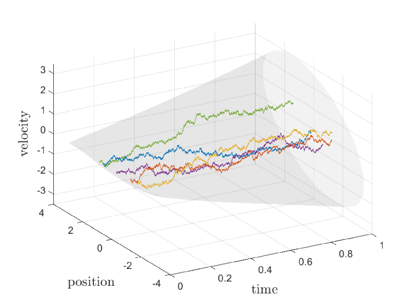
Figure 1: Sample paths for the uncontrolled evolution.

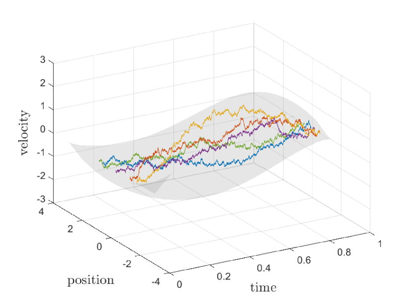
Figure 2: Sample paths for the controlled evolution.

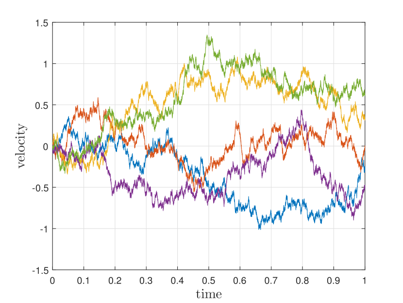
Figure 3: Sample paths for the uncontrolled velocity.

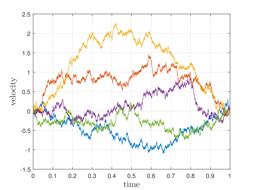
Figure 4: Sample paths for the controlled velocity.

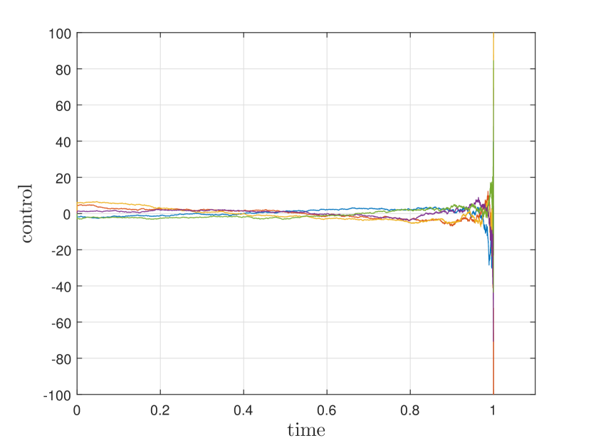
Figure 5: Control inputs.

VII Concluding remarks and future directions

We have addressed the problem of steering a linear stochastic system between two end-point degenerate Gaussian distributions. Specifically, we have shown that there exists an admissible control steering the system to the desired final configuration, and that this can be expressed in closed form. Moreover, the resulting controlled evolution belongs to the same reciprocal class of the uncontrolled one.

The issue of “optimality” is rather subtle as, necessarily, any control strategy steering the system to the desired degenerate marginal grows unbounded at $t=T$. This same issue arose in the case of fixed boundary conditions in [13], i.e., Dirac marginals, and was addressed by controlling $\zeta_{t}$ over the smaller time interval $T-\varepsilon$ while introducing a suitable penalty term $F(\zeta_{T-\varepsilon})$.

An alternative strategy, in the spirit of what has already been presented in the present paper, is to define “optimality” of the control indirectly by expressing it as the limit of a standard (non-degenerate) case for a suitable vanishing perturbation (brought in to remove the degeneracy) and requiring that the limit is independent of the chosen perturbation.

Interestingly, in the special case where degeneracy appears at one of the terminal points, a natural choice for the optimal control is inherited by the time-symmetry of the problem. Specifically, when the starting marginal at $t=0$ is degenerate, and therefore $\Sigma_{0}$ singular while $\Sigma_{T}$ is not, one would not perceive any issue when comparing controls. Indeed, in the forward time-direction admissible controls only need to have finite energy and thereby can be compared directly. When the degeneracy is reversed, with $\Sigma_{T}$ being singular and $\Sigma_{0}$ not, then the forward-in-time controls are unbounded but the backwards-in-time are not and can be compared for deciding on the optimal one and the corresponding probability law on paths. The probability law on the paths does not give a preference to a time-arrow and can be viewed either way. Thus, it induces a unique choice for the corresponding infinite-energy control in the forward-in-time direction. Optimality of the forward-in-time control can then be claimed on this basis (optimality of the law).

Comparing control strategies in general, when the energy required is infinite, appears to require a deeper exploration and it is hoped that it will be revisited in future work.

-A Proof of Proposition 2

Proof.

As in [6] we introduce the following change of variables:

$$x(t)=N(T,0)^{-1/2}\Phi(0,t)\xi_{t}$$

where $N(\cdot,\cdot)$ is the controllability Gramian of the system. Under this new coordinates system we have that

$$\tilde{\Sigma}_{0,\text{new}}=N(T,0)^{-1/2}\tilde{\Sigma}_{0}N(T,0)^{-1/2},$$

$$\tilde{\Sigma}_{T,\text{new}}=N(T,0)^{-1/2}\Phi(0,T)\tilde{\Sigma}_{T}\Phi(0,T)^{\prime}N(T,0)^{-1/2},$$

$$P_{\text{new}}(t)=N(T,0)^{-1/2}\Phi(0,t)P(t)\Phi(0,t)^{\prime}N(T,0)^{-1/2}.$$

Then, by the very same argument in [6], we obtain the following two sets of final conditions for the system of Lyapunov differential equations (4):

$$P^{\pm}(T)= \Phi(T,0)N(T,0)^{1/2}\tilde{\Sigma}_{T,\text{new}}^{1/2}\bigg{(}\tilde{\Sigma}_{T}+\frac{1}{2}I\pm$$

$$\left(\tilde{\Sigma}_{T,\text{new}}^{1/2}\tilde{\Sigma}_{0,\text{new}}\tilde{\Sigma}_{T,\text{new}}^{1/2}+\frac{1}{4}I\right)^{1/2}\bigg{)}^{-1}\tilde{\Sigma}_{T,\text{new}}^{1/2}N(T,0)^{1/2}\Phi(T,0)^{\prime}$$

$$Q^{\pm}(T) =(\tilde{\Sigma}_{T}^{-1}-P^{\pm}(T)^{-1})^{-1}$$

and again by mimicking [6] it can be shown that $P^{-}(t)$ and $Q^{-}(t)$ are non-singular on $[0,T]$.

To recover the formula in the statement let us define $G:=\tilde{\Sigma}_{T}^{1/2}\Phi(0,T)^{\prime}N(T,0)^{-1/2}$ so that $\tilde{\Sigma}_{T,\text{new}}=G^{\prime}G$. Then, there exists an orthogonal matrix $U$ such that $UG=G^{\prime}U^{\prime}$, $UG\succ 0$. Thus, $UG$ is the unique symmetric positive definite square root of $\tilde{\Sigma}_{T,\text{new}}$. Substituting in the expression for $P^{-}(T)$ and rearranging terms,

$$P(T)= \Big{(}\Phi(0,T)^{\prime}N^{-1}\Phi(0,T)$$

$$+\frac{1}{2}\Sigma_{T}^{-1}-\Phi(0,T)^{\prime}N^{-1/2}(UG)^{-1}\Big{(}UGN^{-1/2}\Sigma_{0}N^{-1/2}G^{\prime}U^{\prime}$$

$$+\frac{1}{4}I\Big{)}(G^{\prime}U^{\prime})^{-1}N^{-1/2}\Phi(0,T)\Big{)},$$

where $N:=N(T,0)$. Finally, to recover the formula in the statement it is enough to observe that $M(T,0)=\Phi(T,0)N(T,0)\Phi(T,0)^{\prime}$ and that the following equality holds:

$$U^{\prime}\Big{(} UGN^{-1/2}\Sigma_{0}N^{-1/2}G^{\prime}U^{\prime}+\frac{1}{4}I\Big{)}^{1/2}U$$

$$=\Big{(}\Sigma_{T}^{1/2}M(T,0)^{-1}\Phi(T,0)\Sigma_{0}\Phi(T,0)^{\prime}M(T,0)^{-1}\Sigma_{T}^{1/2}+\frac{1}{4}I\Big{)}^{1/2}.$$

∎

-B Proof of Proposition 5

Proof.

We show the result for $P(0)$; the result for $Q(T)$ is completely symmetric.

For $\varepsilon_{0}>0$ Theorem 1 applies and the following holds

$$\Sigma_{0,\varepsilon_{0}}(I+Q_{\varepsilon_{0}}(0)^{-1}P_{\varepsilon_{0}}(0))=P_{\varepsilon_{0}}(0).$$ (23)

Moreover, we recall that in view of Proposition 3 $\lim_{\varepsilon_{0}\rightarrow 0}Q_{\varepsilon_{0}}(0)^{-1}$ is well defined. We partition $P_{\varepsilon_{0}}(0)$ and $Q_{\varepsilon_{0}}(0)^{-1}$ conformally to $\Sigma_{0}$ as

$$P_{\varepsilon_{0}}(0):=\begin{bmatrix}R+O(\varepsilon_{0})&S+O(\varepsilon_{0})\\ S^{\prime}+O(\varepsilon_{0})&V+O(\varepsilon_{0})\end{bmatrix},\;Q_{\varepsilon_{0}}(0)^{-1}:=\begin{bmatrix}E_{\varepsilon_{0}}&F_{\varepsilon_{0}}\\ F_{\varepsilon_{0}}^{\prime}&G_{\varepsilon_{0}}\end{bmatrix}.$$

and by substituting in (23) and taking the limit we obtain

$$\begin{bmatrix}\Lambda_{0}&0\\ 0&0\end{bmatrix}\left(\begin{bmatrix}I&0\\ 0&I\end{bmatrix}+\begin{bmatrix}E&F\\ F^{\prime}&G\end{bmatrix}\begin{bmatrix}R&S\\ S^{\prime}&V\end{bmatrix}\right)=\begin{bmatrix}R&S\\ S^{\prime}&V\end{bmatrix}$$

where $\lim_{\varepsilon_{0}\rightarrow 0}E_{\varepsilon_{0}}=E$, $\lim_{\varepsilon_{0}\rightarrow 0}F_{\varepsilon_{0}}=F$ and $\lim_{\varepsilon_{0}\rightarrow 0}G_{\varepsilon_{0}}=G$.
Then, by solving the associated system of equations in $R,\,S$ and $V$, we get that $S=V=0$ and that

$$\Lambda_{0}+\Lambda_{0}ER=R.$$ (24)

Finally, from (24) it is immediate to see that $R$ is non-singular as $\Lambda_{0}=(I-\Lambda_{0}E)R$ is positive definite by definition. ∎

References

- [1] F. Badawi, A. Lindquist, and M. Pavon. A stochastic realization approach to the smoothing problem. IEEE Trans. Aut. Control, 24(6):878–888, 1979.
- [2] E. Bakolas. Optimal covariance control for discrete-time stochastic linear systems subject to constraints. In 2016 CDC IEEE 55th Conference, pages 1153–1158. IEEE, 2016.
- [3] A. Beghi. Continuous-time Gauss-Markov processes with fixed reciprocal dynamics. Journal of Mathematical Systems Estimation and Control, 7(3):343–366, 1997.
- [4] Y. Chen and T. Georgiou. Stochastic bridges of linear systems. IEEE Transactions on Automatic Control, 61(2):526–531, 2016.
- [5] Y. Chen, T. T. Georgiou, and M. Pavon. On the relation between optimal transport and Schrödinger bridges: A stochastic control viewpoint. Journal of Optimization Theory and Applications, 169(2):671–691, 2016.
- [6] Y. Chen, T. T. Georgiou, and M. Pavon. Optimal steering of a linear stochastic system to a final probability distribution, Part I. IEEE Trans. Automat. Contr., 61(5):1158–1169, 2016.
- [7] Y. Chen, T. T. Georgiou, and M. Pavon. Optimal steering of a linear stochastic system to a final probability distribution, Part II. IEEE Transactions on Automatic Control, 61(5):1170–1180, 2016.
- [8] Y. Chen, T. T. Georgiou, and M. Pavon. Optimal transport over a linear dynamical system. IEEE Transactions on Automatic Control, 62(5):2137–2152, 2017.
- [9] Y. Chen, T. T. Georgiou, and M. Pavon. Optimal steering of a linear stochastic system to a final probability distribution, Part III. IEEE Transactions on Automatic Control, 63(9):3112–3118, 2018.
- [10] E. Collins and R. Skelton. A theory of state covariance assignment for discrete systems. IEEE Trans. on Automatic Control, 32(1):35–41, 1987.
- [11] P. Dai Pra. A stochastic control approach to reciprocal diffusion processes. Applied mathematics and Optimization, 23(1):313–329, 1991.
- [12] P. Dai Pra and M. Pavon. On the Markov processes of Schrödinger, the Feynman-Kac formula and stochastic control. In Realization and Modelling in System Theory, pages 497–504. Springer, 1990.
- [13] W. H. Fleming and S.-J. Sheu. Stochastic variational formula for fundamental solutions of parabolic pde. Applied Mathematics and Optimization, 13(1):193–204, 1985.
- [14] H. Föllmer. Random fields and diffusion processes. In P. L. Hennequin, editor, Ècole d’Ètè de Probabilitès de Saint-Flour XV-XVII, volume 1362, pages 102–203. Springer, 1988.
- [15] I. Gentil, C. Léonard, and L. Ripani. About the analogy between optimal transport and minimal entropy. Ann. Fac. Sci. Toulouse Math. (6), 26(3):569–601, 2017.
- [16] A. Halder and E. D. Wendel. Finite horizon linear quadratic gaussian density regulator with Wasserstein terminal cost. In American Control Conference (ACC), 2016, pages 7249–7254. IEEE, 2016.
- [17] A. Hotz and R. E. Skelton. Covariance control theory. International Journal of Control, 46(1):13–32, 1987.
- [18] B. Jamison. Reciprocal processes. Zeitschrift. Wahrsch. Verw. Gebiete, 30(1):65–86, 1974.
- [19] C. Léonard. From the Schrödinger problem to the Monge–Kantorovich problem. Journal of Functional Analysis, 262(4):1879–1920, 2012.
- [20] C. Léonard. A survey of the Schrödinger problem and some of its connections with optimal transport. Discrete Contin. Dyn. Syst. A, 34(4):1533–1574, 2014.
- [21] B. C. Levy and A. J. Krener. Dynamics and kinematics of reciprocal diffusions. Journal of Mathematical Physics, 34(5):1846–1875, 1993.
- [22] T. Mikami. Monge’s problem with a quadratic cost by the zero-noise limit of h-path processes. Probability Theory and Related Fields, 129(2):245–260, 2004.
- [23] T. Mikami and M. Thieullen. Duality theorem for the stochastic optimal control problem. Stoch. Proc. Appl., 116(12):1815–1835, 2006.
- [24] T. Mikami and M. Thieullen. Optimal transportation problem by stochastic optimal control,. SIAM Journal of Control and Optimization, 47(3):1127–1139, 2008.
- [25] D. Revuz and M. Yor. Continuous Martingales and Brownian Motion (2nd ed.). Springer, 1999.
- [26] E. Schrödinger. Über die Umkehrung der Naturgesetze. Sitzungsberichte der Preuss Akad. Wissen. Phys. Math. Klasse, Sonderausgabe, IX:144–153, 1931.
- [27] E. Schrödinger. Sur la théorie relativiste de l’électron et l’interprétation de la mécanique quantique. Ann. Inst. H. Poincaré, 2(4):269–310, 1932.