Dynamic Vehicle Routing Problem:
A Monte Carlo approach

Abstract

In this work we solve the Dynamic Vehicle Routing Problem (DVRP). DVRP is a modification of the Vehicle Routing Problem, in which the clients’ requests (cities) number and location might not be known at the beginning of the working day Additionally, all requests must be served during one working day by a fleet of vehicles with limited capacity. In this work we propose a Monte Carlo method (MCTree), which directly approaches the dynamic nature of arriving requests in the DVRP. The method is also hybridized (MCTree+PSO) with our previous Two–Phase Multi-swarm Particle Swarm Optimization (2MPSO) algorithm.

Our method is based on two assumptions. First, that we know a bounding rectangle of the area in which the requests might appear. Second, that the initial requests’ sizes and frequency of appearance are representative for the yet unknown clients’ requests. In order to solve the DVRP we divide the working day into several time slices in which we solve a static problem. In our Monte Carlo approach we randomly generate the unknown clients’ requests with uniform spatial distribution over the bounding rectangle and requests’ sizes uniformly sampled from the already known requests’ sizes. The solution proposal is constructed with the application of a clustering algorithm and a route construction algorithm.

The MCTree method is tested on a well established set of benchmarks proposed by Kilby et al. [1, 2] and is compared with the results achieved by applying our previous 2MPSO [3] algorithm and other literature results. The proposed MCTree approach achieves a better time to quality trade–off then plain heuristic algorithms. Moreover, a hybrid MCTree+PSO approach achieves better time to quality trade–off then 2MPSO for small optimization time limits, making the hybrid a good candidate for handling real world scale goods delivery problems.

1 Introduction

The static Vehicle Routing Problem (VRP) has been introduced in 1959 by Dantzig and Ramser [4]. The VRP is a generalization of the Traveling Salesman Problem, where the weighted nodes representing requests are served by the fleet of vehicles with limited capacity. Since its introduction the problem has received much attention in the literature (e.g. Fisher and Jaikumar 1981 [5], Christofides and Beasley 1984 [6], Taillard 1993 [7], Toth and Vigo 2001 [8]). Moreover, the problem itself has been generalized in various ways in order to model certain real-world scenarios, such as: VRP with Time Windows [9], VRP with Pickup and Delivery [10], Stochastic VRP [11], VRP with Heterogeneous Fleet [12] etc. One of the most recent generalizations is the Vehicle Routing Problem with Dynamic Requests, which is more often simply called the Dynamic Vehicle Routing Problem (DVRP).

Although the quality of the DVRP solutions has been successfully improved in the recent years by the two meta-heuristic based algorithms: Two–Phase Multi-swarm Particle Swarm Optimization (2MPSO) [3] and Multi-environmental cooperative parallel metaheuristics (MEMSO) [13], the computational effort of obtaining good solutions might be two high for the real world scenarios, were one considers several thousand requests and a few hundred vehicles during one working day.

On the other hand solutions achieved by a fast heuristic approach might be of a poor quality. Therefore, in this paper the authors investigate a method of improving heuristic algorithm results in dynamic environment by generating artificial data and assess the time-to-quality ratio of their various configurations.

The rest of the paper is organized as follows. Section 2 gives the definition of the DVRP considered in this paper. Section 3 presents some general remarks for solving dynamic problems and describes the role of the cut-off time parameter. Sections 4, 5, 6 and 7 describe generating of artificial requests procedure and the MCTree, 2MPSO and MCTree+PSO algorithms used to solve the problem, respectively. Section 8 presents the results obtained by the proposed method and compared with literature results. Finally, Section 9 concludes the paper.

Table 1: Symbols used in this paper

Symbol	Type	Description
Dynamic Vehicle Routing Problem
$C$	Series	Clients requests
$C^{\prime}_{t}$	Series	Artificial clients requests generated at time $t$
$c_{i}$	Client	$i$th client (quadruple of size, location, duration and time)
$V$	Series	Fleet of vehicles
$v_{i}$	Vehicle	$i$th vehicle
$n$	$\mathbb{Z_{+}}$	Number of vehicles
$m$	$\mathbb{Z_{+}}$	Number of clients
$m_{t}$	$\mathbb{Z_{+}}$	Number of clients known at the time $t$
$m^{\prime}_{t}$	$\mathbb{Z_{+}}$	Number of artificial clients generated at the time $t$
$l_{i}$	$\mathbb{R}^{2}$	Location of the $i$th client
$l_{i}.x$	$\mathbb{R}$	$x$ coordinate of the $i$th client
$l_{i}.y$	$\mathbb{R}$	$y$ coordinate of the $i$th client
$L^{\prime}_{t}$	Series	Artificial clients requests’ locations generated at time $t$
$u_{i}$	$\mathbb{R_{+}}$	Cargo unloading time for the $i$th client
$\mathbf{{{\bar{u}}_{m_{t}}}}$	$\mathbb{R_{+}}$	Average unloading time for the first $m_{t}$ clients
$s_{i}$	$\mathbb{R_{+}}$	Size of the $i$th request
$S^{\prime}_{t}$	Series	Artificial clients requests’ sizes generated at time $t$
$t_{i}$	$\mathbb{R}$	Time when the request of the $i$th client becomes known
$l_{0}$	$\mathbb{R}^{2}$	Location of the depot
$\rho(i,j)$	$\mathbb{R}$	Distance between $l_{i}$ and $l_{j}$
$t_{start}$	$\mathbb{R}$	Depot opening time
$t_{end}$	$\mathbb{R}$	Depot closing time
$cap$	$\mathbb{R_{+}}$	Capacity of the vehicle
$sp$	$\mathbb{R_{+}}$	Speed of the vehicle
$\mathbf{r_{i}}$	Series	Route of the $i$th vehicle (indexes of subsequent locations)
$m_{i}$	$\mathbb{Z_{+}}$	Number of locations assigned to $i$th vehicle
$arv_{r_{i,j}}$	$\mathbb{R}$	Arrival time of the $i$th vehicle at its $j$th client
$t$	$\mathbb{R}$	Time ($\forall_{t}t_{start}\leq t\leq t_{end}$)
Problem Solving Framework
$T_{CO}$	$[0,1]$	New requests arrival cut-off time; fraction of the working day
Particle Swarm Optimization
$n$	$\mathbb{Z}$	Search space dimension
$t$	$\mathbb{Z}$	Iteration number
$x_{t}$	$\mathbb{R}^{n}$	Particle’s location in $t$th iteration
$v_{t}$	$\mathbb{R}^{n}$	Particle’s velocity in $t$th iteration
$g$	$\mathbb{R}$	Best neighbor location attraction factor
$l$	$\mathbb{R}$	Historically best location attraction factor
$a$	$\mathbb{R}$	Particles’ velocity inertia coefficient
$u^{(i)}$	$\mathbb{R}^{n}$	a random vector with $n$-dimensional uniform distribution
$x^{i}_{best}$	$\mathbb{R}^{n}$	the best location visited by the $i$th particle
$x^{n[i]}_{best}$	$\mathbb{R}^{n}$	the best location visited by the neighbors of the $i$th particle

2 DVRP Definition

In the class of Dynamic Vehicle Routing Problems discussed in this article one considers a fleet $V$ of $n$ vehicles and a series $C$ of $m$ clients (requests) to be served (a cargo is to be delivered to them).

The fleet of vehicles is homogeneous. Vehicles have identical capacity $cap$ and the same speed $sp$.

The cargo is taken from a single depot which has a certain location $l_{0}$ and working hours from $t_{start}$ to $t_{end}$.

Each client $c_{i},i=1,\ldots,m$ has a given location $l_{i}$, time $t_{i}$ (a point in time when the $i$th request becomes available ($t_{start}\leq t_{i}\leq t_{end}$)), time $u_{i}$ (time required to unload the cargo), and size of the request $s_{i}$ ($s_{i}\leq cap$).

A travel distance $\rho(i,j)$ is the Euclidean distance between $l_{i}$ and $l_{j}$ on the $\mathbb{R}^{2}$ plane, $i,j=0,\ldots,m$.

The route $\mathbf{r_{i}}$ of vehicle $v_{i}$ is a series of $r_{i,j}$ indexes of clients, where the first $r_{i,1}=0$ and last $r_{i,m_{i}}=0$ are the identifiers of the depot. Additionally, the series of $arv_{r_{i,j}}$ time points defines vehicle’s time of arrival at those locations.

The goal of the DVRP is to serve the clients (requests), according to their defined time and size constraints, with minimal total cost (travel distance). Formally, the optimization goal can be written as:

$$\text{min}\sum\limits_{i=1}^{n}\sum\limits_{j=2}^{m_{i}}\rho(r_{i,j-1},r_{i,j})$$ (1)

The feasible solution must fulfill the following constrains:

• Each client is served by only one vehicle (requests may not be divided):

  $$\forall_{j\in\{1,2,\ldots m\}}\exists!_{i\in\{1,2,\ldots n\}}j\in\mathbf{r_{i}}$$ (2)

• the vehicle cannot arrive at the location of the next request before the previous one is served:

  $$\forall_{i\in\{1,2,\ldots n\}}\forall_{j\in\{2,3\ldots m_{i}\}}arv_{r_{i,j}}\geq arv_{r_{i,j-1}}+u_{r_{i,j-1}}+\rho(r_{i,j-1},r_{i,j})\\$$ (3)

• the vehicle cannot leave the previous location before the next one is known:

  $$\forall_{i\in\{1,2,\ldots n\}}\forall_{j\in\{2,3\ldots m_{i}\}}arv_{r_{i,j}}\geq t_{r_{i,j}}+\rho(r_{i,j-1},r_{i,j})\\$$ (4)

• the vehicle must return to the depot before closing time:

  $$\forall_{i\in\{1,2,\ldots n\}}arv_{r_{i,m_{i}}}\leq t_{end}\\$$ (5)

• the vehicle must not leave the depot before opening time:

  $$\forall_{i\in\{1,2,\ldots n\}}arv_{r_{i,1}}\geq t_{start}\\$$ (6)

• the capacity of the vehicle must not be exceeded between two subsequent visits to the depot:

  $$\forall_{i\in\{1,2,\ldots n\}}\forall_{j_{1}<j_{2}<j_{3}\in\{1,2\ldots m_{i}\}}r_{i,j_{1}}=0\wedge r_{i,j_{3}}=0\wedge r_{i,j_{2}}\neq 0\Rightarrow\sum\limits_{j=j_{1}+1}^{j_{3}-1}s_{r_{i,j}}\leq cap\\$$ (7)

3 Solving the DVRP

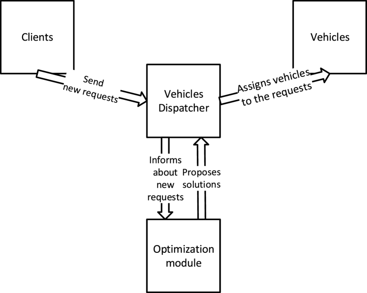
Figure 1: The general framework for solving DVRP

There are two general approaches to solving dynamic optimization problems. In the first one the optimization algorithm is notified every time there is a change in the problem instance. In the second approach time is divided into a discrete slices and the algorithm is run once for each time slice. Furthermore, the problem instance is considered ”frozen” during the whole time slice, i.e. any potential changes introduced during the current time slot are handled in the next algorithm’s run (in the subsequent time slice period).

Another important property of a given dynamic problem is a degree of dynamism (i.e. the ratio of the amount of information unknown at the beginning of the optimization process to the total amount of information provided during the optimization). In the case of the DVRP this property may be measured by the number of requests unknown at the beginning of the working day divided by the total number of requests in the given problem instance. In the DVRP the degree of dynamism is a function of a parameter called cut–off time discussed further in this section.

3.1 General DVRP Framework

Regardless of the approach and the degree of dynamism, the whole system for solving the DVRP may be depicted as in Fig. 1, where the Optimization module (topic of this paper) acts as a service for the Vehicles Dispatcher (VD) (a person or a system). Optimization module presents VD with the best found solution on the basis of the provided data.

3.2 Cut–off Time

As mentioned before, an important DVRP parameter which has a direct impact on the degree of dynamism of a given problem instance, is the cut–off time factor. It defines the part of the requests set that is known at the beginning of the working day. In the real (practical) situations the requests received after this time threshold are moved to be served at the subsequent working day. In the one-day-horizon simulations presented in this paper (as well as in practically all other papers referring to Kilby et al.’s benchmarks [2]) the requests located after the cut–off time limit are simply treated as being known at the beginning of the current day - they compose an initial instance of the DVRP being solved.

3.3 Benchmark Configuration and Optimization Settings

In this article we follow the approach with dividing working day into discrete time slices and running optimization algorithm in each time slice for a ”frozen” static VRP instances. This approach in the context of the DVRP, was proposed by Kilby et al. [1] and has been followed in our previous work with the Particle Swarm Optimization algorithm [14, 3].

In order to assure a possibility of direct comparison of the obtained results with our previous work and with other literature results [15, 16, 13, 17, 18, 19, 20], the cut–off time is set in the middle of a depot’s working hours.

4 Requests generation

In order to approach the dynamic nature of the problem, in each time slice occurring prior to the cut-off time a set of randomly generated requests is added to the currently known ones. Thus, the (D)VRP is solved from scratch in the subsequent time slices with decreasing amount of unknown requests and increasing amount of fixed assignments of vehicles to the requests (due to advancing time). In each time slice it is assumed that we know the maximum spatial range in which the requests may be located (see Eq. (11)) and that the frequency of the requests arrival during the remaining part of the working day will be the same as up till the current point in time (see Eq. (9)). Therefore, new requests are generated uniformly in time and space and their size is uniformly sampled from the already known requests (see Eq. (10)).

$C^{\prime}_{t}$ is a quadruple of sizes, locations, availability times (all set to the current time) and unload times (all set to the average known unload time).

$$C^{\prime}_{t}:=(S^{\prime}_{t},L^{\prime}_{t},\{{t,\ldots,t}\},\{\mathbf{{{\bar{u}}_{m_{t}}}},\ldots\mathbf{{{\bar{u}}_{m_{t}}}}\})$$ (8)

The number $m^{\prime}_{t}$ of the generated $C^{\prime}_{t}$ requests at time $t$, is computed as follows:

$$m^{\prime}_{t}=m_{t}\dfrac{T_{CO}(t_{end}-t_{start})+t_{start}-t}{T_{CO}(t_{end}-t_{start})-t_{start}+t}$$ (9)

The size of the requests is sampled uniformly from the known requests’ sizes:

$$S^{\prime}_{t}\sim U(\{s_{1},s_{2},\ldots,s_{m_{t}}\})$$ (10)

The location of the requests is generated uniformly over the bounding rectangle of all of the requests:

$$L^{\prime}_{t}\sim U([\min\limits_{i_{1}\in\{1,2,\ldots,m\}}(l_{i_{1}}.x),\max\limits_{i_{2}\in\{1,2,\ldots,m\}}(l_{i_{2}}.x)]\times[\min\limits_{i_{3}\in\{1,2,\ldots,m\}}(l_{i_{3}}.y),\max\limits_{i_{4}\in\{1,2,\ldots,m\}}(l_{i_{4}}.y)])$$ (11)

Uniform distribution models the assumption of knowing only the spatial boundaries in which new requests can appear.

1:   {$E$ a set of weighted edges, weights represent the distances between nodes}

2:   {$V$ a set of weighted nodes, weights represent the size of the requests}

3:   {$CAPACITY$ a constant representing the capacity of a single vehicle}

4:  $T_{clusters}\Leftarrow CreateSeparateTrees(V)$

5:  $E_{sort}\Leftarrow SortByWeightInAscendingOrder(E)$

6:  for all $(v_{1},v_{2})\in E_{sort}$ do

7:     if $Tree(v_{1})\neq Tree(v_{2})$  then

8:        if $Weight(Tree(v_{1}))+Weight(Tree(v_{2}))\leq CAPACITY$  then

9:           if $Distance(v_{1},v_{2})\leq Distance(v_{1},Depot)$ and $Distance(v_{1},v_{2})\leq Distance(v_{2},Depot)$  then

10:              $T_{clusters}\Leftarrow T_{clusters}\setminus\{Tree(v_{1}),Tree(v_{2})\}$

11:              $T_{clusters}\Leftarrow T_{clusters}\cup\{Tree(v_{1})\cup Tree(v_{2})\}$

12:           end if

13:        end if

14:     end if

15:  end for

Figure 2: Pseudocode of the modified Kruskal algorithm for solving a capacitated clustering task.

1:  while true do

2:     for all $j_{1}\in\{2,3,\ldots,m_{i}-1\}$ do

3:        if $c_{r_{i,j_{1}}}$ is fixed  then

4:           continue

5:        end if

6:        for all $j_{2}\in\{j_{1}+1,j_{1}+2,\ldots,m_{i}\}$ do

7:           if $\rho(r_{i,j_{1}-1},r_{i,j_{1}})+\rho(r_{i,j_{2}-1},r_{i,j_{2}})<\rho(r_{i,j_{1}-1},r_{i,j_{2}-1})+\rho(r_{i,j_{1}},r_{i,j_{2}})$  then

8:              for all $j_{3}\in\{j_{1},j_{1}+1,\ldots,j_{2}-1\}$, $j_{4}\in\{j_{2}-1,j_{2}-2,\ldots,j_{1}\}$ do

9:                 $r_{i,j_{3}}\leftrightarrow r_{i,j_{4}}$

10:                 if $j_{4}\leq j_{3}$ then

11:                    break

12:                 end if

13:              end for

14:           end if

15:        end for

16:     end for

17:     if nothing to optimize then

18:        break

19:     end if

20:  end while

Figure 3: Pseudocode of the 2-OPT algorithm for optimizing the route $\mathbf{r_{i}}$ of the $i$th vehicle.

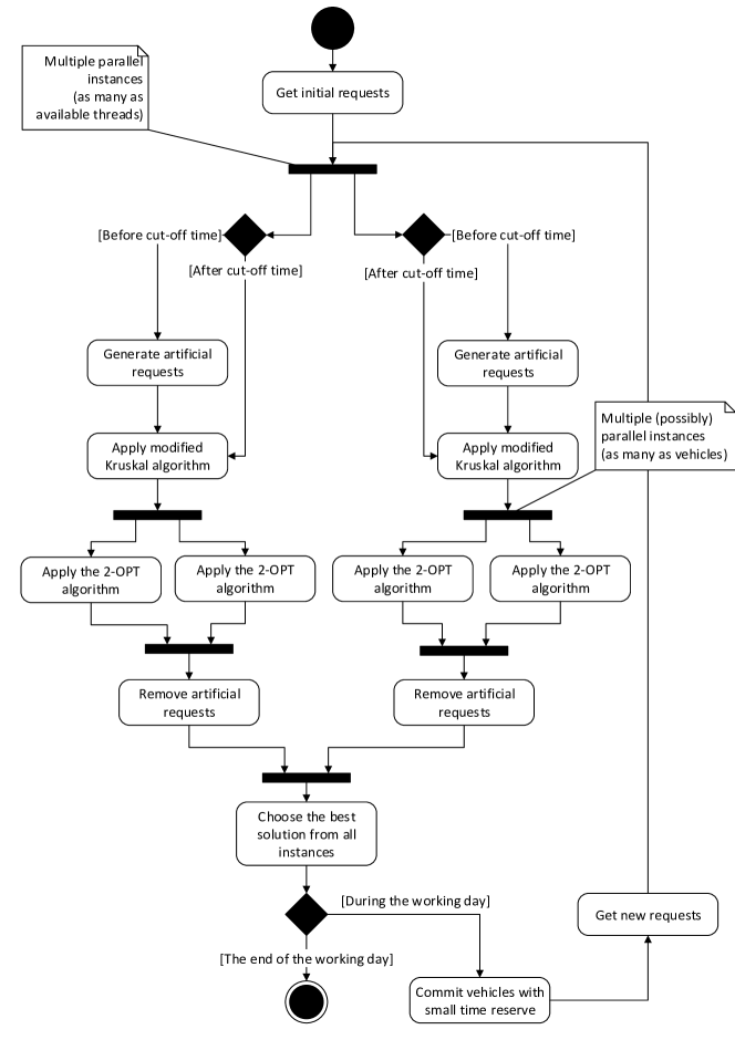
Figure 4: Activity diagram of the MCTree algorithm.

5 MCTree algorithm

The MCTree algorithm for solving the (D)VRP is a sequence of two heuristic algorithms. In the first step, a capacitated clustering problem is solved by the usage of a modified version of the Kruskal algorithm [21], thus creating a requests-to-vehicles assignment. In the second step, the partially random routes of the vehicles are optimized with the 2–OPT algorithm [22]. In that step routes are optimized independently within each single cluster of the requests.

5.1 Requests Assignment Optimization (Clustering)

The goal of the modified Kruskal algorithm is to create a forest with each tree representing the clients assigned to one vehicle. Please note, that because of the limited sum of nodes’ weights in each tree the final forest graph might not be a sub-graph of the minimum spanning tree created by a standard Kruskal algorithm.

The pseudo-code for the modified Kruskal algorithm is presented in Fig. 2. There are two modifications made in the standard algorithm in order to achieve solutions for the (D)VRP. The first modification is in the line 8, stating that two trees cannot be joined if the sum of their nodes’ weights would exceed the capacity of the vehicle. The second modification (line 9) is an experimentally chosen heuristic rule, preventing the creation of the routes covering large areas and (possibly) overlapping with others.

Please note, that creating the initial clusters (line 4), takes into account clients with fixed assignment to a given vehicle and a set of edges (sorted in line 5) consists only of the edges between all non-fixed clients and the fixed and non-fixed clients, without the edges between the fixed clients (so the problem size decreases size after a certain point of the day).

5.2 Routes Optimization

The goal of the 2–OPT algorithm is creation of an acceptable quality routes for each of the vehicles. The 2–OPT algorithm checks all pairs of the non-fixed edges for the possibility of minimizing the route length by swapping their ends.

Pseudocode of the 2-OPT algorithm is presented in Fig. 3. The 2-OPT executes as long as the route is improved by exchanging two edges (line 7) and the part of the route between the exchanged edges is reversed(line 9).

The algorithm had to be slightly changed in order to incorporate the dynamic nature of the optimized problem (i.e. the initial part of the route becomes fixed). Instead of iterating over the whole route, the optimization starts from the first non-fixed client $c_{r_{i,j_{1}}}$ of the solution for a given vehicle $\mathbf{r_{i}}$ (line 3).

5.3 Algorithm Architecture

The generation of the artificial requests, the clustering algorithm and the route optimization algorithm are the main building blocks of the MCTree method.

The activity diagram of the MCTree algorithm is depicted in Fig. 4. In each time slice the algorithm is run in separate multiple parallel instances (by default as many as available real or virtual CPUs: 8 in the case of Intel Core i7 used in this study). In each of the parallel processes the artificial requests are generated independently. After the generation of the requests, first the Kruskal algorithm and then the 2-OPT algorithm are applied. Finally, the artificial requests are removed from the solution and the best found set of routes among the separate parallel instances is chosen. Subsequently the algorithm advances to the next time slice.

Please note, that the generation of requests is an optional step and can be omitted (such approach is denoted as the Tree algorithm). Also, both the Kruskal and 2-OPT algorithm can be replaced (or enhanced) with another clustering and route optimization algorithms (as will be the case in the approach using Particle Swarm Optimization algorithm (2MPSO)), which is discussed in the next section.

6 2MPSO algorithm

The Two–Phase Multi-swarm Particle Swarm Optimization (2MPSO) algorithm for the DVRP has been introduced by the authors in 2014 [3]. In the 2MPSO algorithm a continuous optimization Particle Swarm Optimization (PSO) algorithm is used for the requests clustering and the vehicles’ routes optimization. Therefore, the authors have proposed a continuous encoding for both the requests-to-vehicle assignment and requests ordering task.

6.1 Continuous DVRP Encoding

The assignment is encoded as a flattened (one dimensional) array of requests’ cluster centers. Each vehicle is associated with a set of such cluster centers, thus all requests belonging to the given clusters are assigned to that vehicle. In order to evaluate the assignment as a set of vehicles’ routes, each set of clients assigned to one vehicle is treated as a random route and optimized with 2–OPT before computing the value of the objective function.

The route ordering for a given vehicle is achieved by sorting the indexes of the vector of the length equal to the number of requests assigned to that vehicle. The rank of the index corresponding to the given requests is defined by the rank of its value in the vector.

Creation of that continuous encodings (together with assignment-to-route conversion) allowed for a direct application of the PSO algorithm to the DVRP.

6.2 Particle Swarm Optimization

PSO is an iterative global optimization meta-heuristic method proposed in 1995 by Kennedy and Eberhart [23] and further studied and developed by many other researchers, e.g., [24, 25, 26]. In short, PSO utilizes the idea of swarm intelligence to solve hard optimization tasks. The underlying idea of the PSO algorithm consists in maintaining the swarm of particles moving in the search space. For each particle the set of neighboring particles which communicate their positions and function values to this particle is defined. Furthermore, each particle maintains its current position and velocity, as well as remembers its historically best (in terms of solution quality) visited location. More precisely, in each iteration $t$, each particle $i$ updates its position $x^{i}_{t}$ and velocity $v^{i}_{t}$ according to the following formulas for the position and velocity update.

The position of a particle is updated according to the following equation:

$$x^{i}_{t+1}=x^{i}_{t}+v^{i}_{t}.$$ (12)

In our implementation of the PSO (based on [27] and [24]) the velocity $v^{i}_{t}$ of a particle $i$ is updated according to the following rule:

$$v^{i}_{t+1}=u^{(1)}_{U[0;g]}(x^{n[i]}_{best}-x^{i}_{t})+u^{(2)}_{U[0;l]}(x^{i}_{best}-x^{i}_{t})+a\cdot v^{i}_{t}\\$$ (13)

where

• $g$ is a neighborhood attraction factor,

• $x^{n[i]}_{best}$ represents the best position (in terms of optimization) found hitherto by the particles belonging to the neighborhood of the $i$th particle,

• $l$ is a local attraction factor,

• $x^{i}_{best}$ represents the best position (in terms of optimization) found hitherto by particle $i$,

• $a$ is an inertia coefficient,

• $u^{(1)}_{U[0;g]}$, $u^{(2)}_{U[0;l]}$ are random vectors with uniform distribution from the intervals $[0,g]$ and $[0,l]$, respectively.

6.3 Similarities to MCTree

The general structure of the 2MPSO algorithm is similar to that of the MCTree:

• in each time step a static instance is optimized in independent parallel instances of the algorithm,

• First, the requests assignment problem is solved (in the case of 2MPSO by solving continuous clustering problem with the PSO algorithm),

• Subsequently, the routes are optimized for each of the vehicles independently (also by applying PSO to continuous route order encoding),

• Finally, the best solution is chosen among the parallel instances of the algorithm.

6.4 Differences with MCTree

The main difference between the 2MPSO and MCTree (apart from the continuous vs. discrete optimization) is the method of approaching the dynamic nature of the DVRP problem. In the MCTree the problem is solved from scratch in each time slice, with a sort of safety buffer for vehicles’ capacities created by generation of artificial requests. In the 2MPSO the solution from the previous time slice is used to generate a few of the solutions in the initial population of PSO and the search space is centered around such a solution. Therefore, 2MPSO relies on the knowledge transfer between the time slices.

6.5 Heuristic Algorithms

In the 2MPSO both Kruskal based clustering and 2–OPT algorithm are heavily used. Kruskal algorithm is used for finding one of the initial solutions in the PSO swarm. 2–OPT algorithm is used for creating the routes from the proposed assignments, allowing for evaluating requests-to-vehicles assignment as the solutions of the VRP.

Please refer to the [3] and [14] for more detailed description and parameter setting of the 2MPSO. Also, please note that in the experiments in this paper the PSO will be used only to improve the requests-to-vehicles assignment (such approach has a better computations time to quality pay off).

7 MCTree+PSO algorithm

The MCTree+PSO algorithm switches from optimizing with the MCTree to 2MPSO, when there are no more unknown requests (i.e. after the cut–off time). The idea of switching after the cut–off time comes from the fact, that that time MCTree changes into a plain heuristic Tree algorithm as there are no more artificial requests to generate. Additionally, the problem to optimize at that time of the working day usually becomes smaller, as at least part of the requests-to-vehicles assignment is already fixed, because the vehicles had to start to deliver the cargo. Therefore, instead of a plain heuristic Tree algorithm the 2MPSO is used as an optimizer in the second part of a working day.

8 Results

Table 2: Comparison of the minimum and the average total routes length achieved by the Tree, MCTree and MCTree with 2MPSO after cut-off time and 2MPSO with the average computation time of about 20 seconds per benchmark. The numbers denote the number of time slices (TS), parallel instances (P) and fitness function evaluations (FFE). In the case of the PSO, the FFE is presented as the number of particles multiplied by the number of iterations.

	Tree		MCTree		MCTree+PSO		2MPSO
	$200TS\times 8P\times 1FFE$		$200TS\times 8P\times 1FFE$		$20TS\times 8P\times 1FFE$+		$40TS\times 8P\times(4\times 28)FFE$
					$20TS\times 8P\times(7\times 49)FFE$
	Min	Avg	Min	Avg	Min	Avg	Min	Avg
c50	673.34	721.51	654.69	700.49	621.27	677.03	566.98	610.47
c75	1049.07	1117.71	1038.80	1123.43	998.72	1066.00	927.22	988.06
c100	1095.82	1193.98	1004.15	1119.42	979.95	1066.44	930.33	1038.53
c100b	828.94	843.07	828.94	836.75	823.23	831.72	828.63	858.75
c120	1072.86	1106.33	1078.23	1109.12	1068.46	1100.28	1071.20	1112.88
c150	1318.78	1463.85	1269.23	1399.93	1223.15	1323.35	1205.80	1306.79
c199	1644.67	1824.89	1571.05	1702.24	1533.68	1601.22	1471.16	1597.98
f71	290.37	348.80	303.49	333.99	288.72	323.85	278.56	310.31
f134	12730.29	13501.66	12719.73	13474.06	12134.30	12473.32	12377.63	12746.26
tai75a	1864.10	2016.29	1929.44	2016.40	1899.17	1980.37	1832.11	1957.01
tai75b	1578.05	1631.85	1523.07	1655.02	1515.71	1582.37	1499.58	1611.63
tai75c	1614.94	1800.66	1570.30	1704.14	1526.75	1657.88	1555.36	1642.58
tai75d	1431.89	1612.26	1430.75	1467.25	1426.39	1456.08	1444.70	1520.84
tai100a	2359.58	2651.78	2441.47	2640.06	2344.78	2532.85	2311.19	2467.77
tai100b	2324.19	2475.94	2297.78	2446.81	2221.67	2344.13	2204.54	2323.27
tai100c	1621.59	1752.83	1619.81	1742.85	1580.00	1676.72	1566.75	1675.89
tai100d	2019.34	2195.64	1909.52	2050.51	1888.07	2000.07	1789.90	1960.36
tai150a	3599.62	3839.13	3555.79	3711.96	3607.78	3763.44	3664.12	3904.32
tai150b	3052.73	3377.34	3145.64	3268.63	3070.44	3226.49	3104.98	3238.59
tai150c	2718.31	2867.25	2707.18	2844.86	2614.59	2725.45	2734.77	2874.79
tai150d	3194.07	3419.10	3100.97	3352.11	3081.26	3200.29	3134.93	3247.68
tai385	29088.27	31144.04	31331.32	33037.53	31876.05	33786.47	30122.29	32433.18
sum	77170.82	82905.91	79031.35	83737.56	78324.14	82395.82	76622.73	81427.94

In order to assess the performance of the algorithms, we use a well established set of benchmarks created by Kilby et al. [1] by converting static instances of VRP used by Christofides [6], Fisher [5] and Taillard [7].

While our previously introduced [3] Two–Phase Multi-swarm Particle Swarm Optimization (2MPSO) outperformed other algorithms using limit on number of fitness function evaluations as a criterion, in this article we shall focus on comparison of the MCTree with the algorithms which use time as the limit for the optimization process: Genetic Algorithm (GA2007) (by Hanshar et al. [17]), Ant Colony Optimization with Large Neighborhood Search (ACOLNS) (by Elhassania et al. [20]) and Genetic Algorithm (GA2014) (by Elhassania et al. [19]).

The tests consisted of running each version of the optimization method 30 times for each of the 22 benchmark instances with four different approaches:

• Tree - in each parallel instance one solution was computed with clustering and route optimization heuristic algorithms without previous generation of the artificial requests,

• MCTree - in each parallel instance one solution was computed with clustering and route optimization heuristic algorithms on the set consisting of real and artificial requests (till the cut-off time),

• MCTree+PSO - till the cut-off time in each parallel instance one solution was computed on the partially artificial set of requests, after the  cut-off time the 2MPSO algorithm was used,

• 2MPSO - 2MPSO algorithm was used for the whole experiment, no artificial requests were generated.

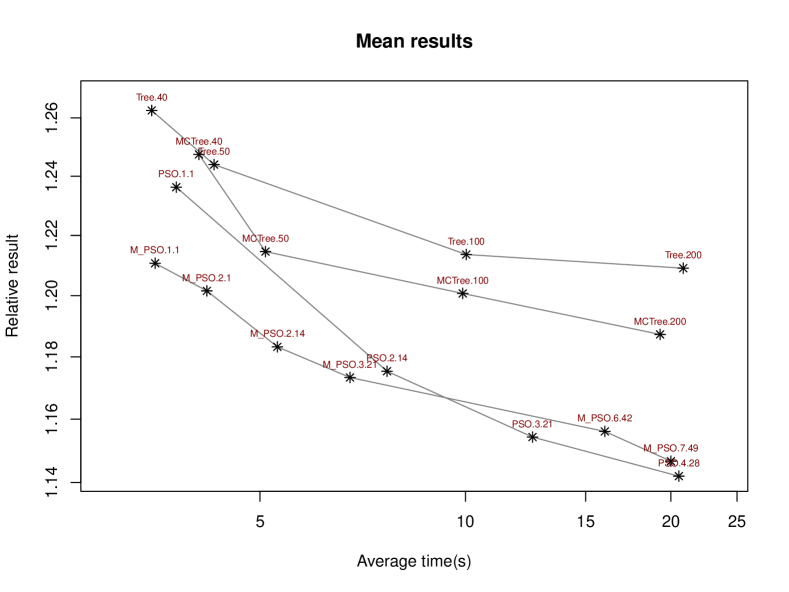
Figure 5: Presentation of the result vs. computation time trade-off for a different sets of parameters for the MCTree and 2MPSO algorithm.

(a) Comparison of the results achieved by a Tree algorithm, with different number of time slices.

(b) Comparison of the results achieved by an MCTree algorithm, with different number of time slices.

(c) Comparison of the results achieved by a 2MPSO algorithm, with different swarm size and number of iterations.

(d) Comparison of the results achieved by an MCTree with PSO at the end algorithms, with different swarm size and number of iterations.

Figure 6: Comparison of the performance of different algorithms. The comparison is done on the basis of relative results (i.e. results divided by the best known result for the given benchmark). The horizontal line represents the mean value achieved by the GA [17] algorithm. Numbers above the boxplots denote the 3rd quartile of the relative results. In each of the subplots leftmost and rightmost results were achived by the algorithm computing on average around 4 seconds per experiment and around 20 seconds per experiment respectively.

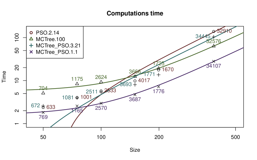
Figure 7: Comparison of the computational effort needed for benchmarks of different number of requests. Labels denote the mean value obtained by the given algorithm for a chosen benchmark size. The regression curves were fitted for the time as a linear function of $m^{2}log(m)$.

Table 3: Comparison of the minimum and the average total routes length achieved by the MCTree with PSO after cut-off time approach and the GA2007, GA2014 and ACOLNS algorithms. The time limit and the processor on which the results were computed is given for each of the algorithms.

	$GA2014$ [19]		$ACOLNS$ [20]		$GA2007$ [17]		$MCTree+PSO$
	1500 seconds		1500 seconds		750 seconds		75 seconds (500 for tai385)
	Intel Core i5@2.4GHz		Intel Core i5@2.4GHz		Intel PentiumIV@2.8GHz		Intel Core i7(2nd)@3.4GHz
	Min	Avg	Min	Avg	Min	Avg	Min	Avg
c50	602.75	618.86	601.78	623.09	570.89	593.42	621.27	677.03
c75	962.79	1027.08	1003.20	1013.47	981.57	1013.45	998.72	1066.00
c100	1000.98	1013.03	987.65	1012.30	961.10	987.59	979.95	1066.44
c100b	899.05	931.35	932.35	943.05	881.92	900.94	823.23	831.72
c120	1328.54	1418.13	1272.65	1451.60	1303.59	1390.58	1068.46	1100.28
c150	1412.03	1461.55	1370.33	1394.77	1348.88	1386.93	1223.15	1323.35
c199	1778.56	1843.06	1717.31	1757.02	1654.51	1758.51	1533.68	1601.22
f71	304.51	323.91	311.33	320.00	301.79	309.94	288.72	323.85
f134	16063.65	16671.17	15557.82	16030.53	15528.81	15986.84	12134.30	12473.32
tai75a	1822.38	1871.46	1832.84	1880.87	1782.91	1856.66	1899.17	1980.37
tai75b	1433.98	1533.63	1456.97	1477.15	1464.56	1527.77	1515.71	1582.37
tai75c	1505.06	1558.70	1612.10	1692.00	1440.54	1501.91	1526.75	1657.88
tai75d	1434.18	1458.93	1470.52	1491.84	1399.83	1422.27	1426.39	1456.08
tai100a	2223.04	2290.05	2257.05	2331.28	2232.71	2295.61	2344.78	2532.85
tai100b	2221.58	2263.46	2203.63	2317.30	2147.70	2215.39	2221.67	2344.13
tai100c	1518.08	1541.25	1660.48	1717.61	1541.28	1622.66	1580.00	1676.72
tai100d	1870.50	2004.78	1952.15	2087.96	1834.60	1912.43	1888.07	2000.07
tai150a	3508.09	3570.51	3436.40	3595.40	3328.85	3501.83	3607.78	3763.44
tai150b	3019.90	3120.57	3060.02	3095.61	2933.40	3115.39	3070.44	3226.49
tai150c	2959.58	3065.73	2735.39	2840.69	2612.68	2743.55	2614.59	2725.45
tai150d	3008.30	3175.37	3138.70	3233.39	2950.61	3045.16	3081.26	3200.29
tai385	40238.00	41319.39	33062.06	35188.99	-	-	31876.05	33786.47
sum	91115.53	94081.97	83632.73	87495.92	49202.73	51088.83	78324.14	82395.82

The comparison of the best performing version of each approach is presented in Table 2, while performance of each of the methods for various parameters setting is presented in Fig. 6. Tree and MCTree algorithms have been run with the working day divided into: $40$, $50$, $100$ and $200$ time slices (see Fig. 6a and Fig. 6b). Dividing working day into $200$ time slices results in running optimization nearly every time when the new request arrive even in the largest benchmarks. Additionally, the total processing time for the largest benchmarks is close to the limit defined by the literature approaches. MCTree+PSO and 2MPSO algorithm have been both run with the working day divided into $40$ time slices (the number tuned for the 2MPSO algorithm). PSO in the MCTree+PSO has been run with the following pairs of swarm size and iterations limit: $1\times 1$, $2\times 1$, $2\times 14$, $3\times 21$, $6\times 42$ and $7\times 49$ (see Fig. 6d). PSO in the 2MPSO has been run with the following pairs of swarm size and iterations limit: $1\times 1$, $2\times 14$, $3\times 21$ and $4\times 28$ (see Fig. 6c). The largest swarm sizes and number of iterations have been chosen in order to stay within the average total processing time of the Tree with $200$ time slices (see Fig. 5). The smaller swarm sizes and number of iterations were tested in order to find algorithms and configurations for the problems were the time limit for processing becomes a crucial constraint (possibly due to the large number of requests).

The average results and the average computational effort for each of the tested parameters set is depicted on the log–log plot of time to result trade-off in Fig. 5. A few chosen cases were additionally depicted in Fig. 7 presenting computational effort for the benchmarks with different number of requests. The regression curves fitted for the time of computations as a linear function of $m^{2}log(m)$, explained at least 95% of the variance for each of the algorithms, thus confirming the theoretical time complexity of all the approaches being $o(m^{2}log(m)$) due to  the computations needed for the clustering (sorting the edges in discrete (MC)Tree case).

From both Fig. 5 and Tab. 2 we could observe, that the MCTree+PSO performed much better than plain MCTree (which performed better than plain Tree algorithm). Therefore, MCTree+PSO is compared with literature results in Table 3. The size of the swarm (7) and the number of iterations (49) for the PSO part of the method were chosen in such way, that the algorithm would not exceed 75 seconds for c199 benchmark and 500 seconds for tai385. The reason being our Intel Core i7@3.4GHz machine is about 10 times faster than the Pentium IV@2.8GHz used for the GA2007 computations (with 750 seconds limit) and about 3 times faster then the Intel Core i5@2.4GHz used for GA2014 and ACOLNS (which were computed with 1500 seconds limit). While Table 3 presents the literature results achieved only by the methods using time as the optimization process limit, the best known values for the benchmarks can be found at the research project [28] website.

9 Discussion and Conclusions

Proposed MCTree algorithm improved the solution which could be achieved by the same heuristic algorithm Tree without the generation of the artificial requests. Further improvement of the average results was possible with the MCTree+PSO hybrid. MCTree+PSO approach for solving DVRP proved to be beneficial over 2MPSO algorithm for small time budget (less then 10 seconds on average for this particular benchmark set on the Intel Core i7 machine). Additionally, it was competitive against both the 2MPSO and GA2007 algorithms, within the larger processing time limit defined by the GA2007. It achieved to get better average results against 2MPSO for the $10$ (out of $22$) benchmark instances and against GA2007 for the $6$ (out of $21$). The average routes computed by MCTree were 1.0144 times longer than GA2007, and 1.0126 times shorter than GA2014 and 1.0178 shorter than ACOLNS while maintaining strict time limit on the largest benchmarks. Probably, this results could be improved for smaller benchmarks (and thus on the average) if the MCTree+PSO algorithm used the time as the limit for the processing for the 2MPSO.

It is important to note that the MCTree+PSO with just single evaluation by the continuous approach has the best average processing time and should be able to process DVRPs with around $10000$ requests in $8$ hours on a single PC (conclusion drawn from the regression curves depicted in Fig. 7). The largest (3 particles and 21 iterations) MCTree+PSO performing better then plain 2MPSO should be able to process problems with around $5400$ requests in that time and 2MPSO with $2$ particles and $14$ iterations (having similar quality of results) problems with around $4700$ requests.

It could be also observed that even such simple generation of the artificial requests improved the performance of the clustering based on the Kruskal algorithm and route construction based on the 2–OPT algorithm.

The proposed approach (generating of artificial requests) might be improved by using another clustering algorithm to solve the assignment of the requests. Another area for further development is more sophisticated generation of artificial requests for a closer resemblance of their spatial distribution.

References

- [1] Kilby, P., Prosser, P., Shaw, P.: Dynamic vrps: A study of scenarios. http://www.academia.edu/2754875/Dynamic_VRPs_A_study_of_scenarios (1998)
- [2] Pankratz, G., Krypczyk, V.: Benchmark data sets for dynamic vehicle routing problems. http://ftp.fernuni-hagen.de/ftp-dir/pub/fachb/wiwi/winf/forschng/resources/montemanni(zip)/montemanni.zip (2009)
- [3] Okulewicz, M., Mańdziuk, J.: Two-Phase Multi-Swarm PSO and the Dynamic Vehicle Routing Problem. In: 2nd IEEE Symposium on Computational Intelligence for Human-like Intelligence. (2014) 86–93
- [4] Dantzig, G.B., Ramser, R.: The Truck Dispatching Problem. Management Science 6 (1959) 80–91
- [5] Fisher, M.L., Jaikumar, R.: A generalized assignment heuristic for vehicle routing. Networks 11(2) (1981) 109–124
- [6] Christofides, N., Beasley, J.E.: The period routing problem. Networks 14(2) (1984) 237–256
- [7] Taillard, É.D.: Parallel iterative search methods for vehicle routing problems. Networks 23(8) (1993) 661–673
- [8] Toth, P., Vigo, D.: The vehicle routing problem. Society for Industrial and Applied Mathematics (2001)
- [9] Solomon, M.M.: Algorithms for the vehicle routing and scheduling problems with time window constraints. Operations research 35(2) (1987) 254–265
- [10] Righini, G.: Approximation algorithms for the vehicle routing problem with pick-up and delivery. Note del Polo-Ricerca 33 (2000)
- [11] Laporte, G., Louveaux, F.V.: Solving stochastic routing problems with the integer L-shaped method. Springer (1998)
- [12] Prins, C.: Efficient heuristics for the heterogeneous fleet multitrip vrp with application to a large-scale real case. Journal of Mathematical Modelling and Algorithms 1(2) (2002) 135–150
- [13] Khouadjia, M.R., Talbi, E.G., Jourdan, L., Sarasola, B., Alba, E.: Multi-environmental cooperative parallel metaheuristics for solving dynamic optimization problems. Journal of Supercomputing 63(3) (2013) 836–853
- [14] Okulewicz, M., Mańdziuk, J.: Application of Particle Swarm Optimization Algorithm to Dynamic Vehicle Routing Problem. In: LNCS. Volume 7895. (2013) 547–558
- [15] Khouadjia, M.R., Sarasola, B., Alba, E., Jourdan, L., Talbi, E.G.: A comparative study between dynamic adapted PSO and VNS for the vehicle routing problem with dynamic requests. Applied Soft Computing 12(4) (2012) 1426–1439
- [16] Khouadjia, M.R., Alba, E., Jourdan, L., Talbi, E.G.: Multi-Swarm Optimization for Dynamic Combinatorial Problems: A Case Study on Dynamic Vehicle Routing Problem. In: Swarm Intelligence. Volume 6234 of Lecture Notes in Computer Science., Berlin / Heidelberg, Springer (2010) 227–238
- [17] Hanshar, F.T., Ombuki-Berman, B.M.: Dynamic vehicle routing using genetic algorithms. Applied Intelligence 27(1) (August 2007) 89–99
- [18] Montemanni, R., Gambardella, L., Rizzoli, A., Donati, A.: A new algorithm for a dynamic vehicle routing problem based on ant colony system. Journal of Combinatorial Optimization 10 (2005) 327–343
- [19] Elhassania, M., Jaouad, B., Ahmed, E.A.: Solving the dynamic vehicle routing problem using genetic algorithms. In: Logistics and Operations Management (GOL), 2014 International Conference on, IEEE (2014) 62–69
- [20] Elhassania, M., Jaouad, B., Ahmed, E.A.: A new hybrid algorithm to solve the vehicle routing problem in the dynamic environment. International Journal of Soft Computing 8(5) (2013) 327–334
- [21] Kruskal, J.B.: On the Shortest Spanning Subtree of a Graph and the Traveling Salesman Problem. Proceedings of the American Mathematical Society (1959) 48–50
- [22] Croes, G.: A method for solving traveling salesman problems. Operations Res. 6 (1958) 791–812
- [23] Kennedy, J., Eberhart, R.: Particle Swarm Optimization. Proceedings of IEEE International Conference on Neural Networks. IV (1995) 1942–1948
- [24] Shi, Y., Eberhart, R.: Parameter selection in particle swarm optimization. Proceedings of Evolutionary Programming VII (EP98) (1998) 591–600
- [25] Shi, Y., Eberhart, R.: A modified particle swarm optimizer. Proceedings of IEEE International Conference on Evolutionary Computation (1998) 69–73
- [26] Cristian, I., Trelea: The particle swarm optimization algorithm: convergence analysis and parameter selection. Information Processing Letters 85(6) (2003) 317–325
- [27] Clerc, M.: Standard PSO 2007 and 2011 (2012)
- [28] Mańdziuk, J., Zadrożny, S., Walȩdzik, K., Okulewicz, M., Świechowski, M.: Adaptive metaheuristic methods in dynamically changing environments. http://www.mini.pw.edu.pl/~mandziuk/dynamic/ (2015)