Guaranteed phase synchronization of hybrid oscillators using symbolic Euler’s method: The Brusselator and biped examples

Abstract

The phenomenon of phase synchronization was evidenced in the 17th century by Huygens while observing two pendulums of clocks leaning against the same wall. This phenomenon has more recently appeared as a widespread phenomenon in nature, and turns out to have multiple industrial applications. The exact parameter values of the system for which the phenomenon manifests itself are however delicate to obtain in general, and it is interesting to find formal sufficient conditions to guarantee phase synchronization. Using the notion of reachability, we give here such a formal method. More precisely, our method selects a portion $S$ of the state space, and shows that any solution starting at $S$ returns to $S$ within a fixed number of periods $k$. Besides, our method shows that the components of the solution are then (almost) in phase. We explain how the method applies on the Brusselator reaction-diffusion and the biped walker examples.

0.1 Introduction

The phenomenon of phase synchronization was evidenced in the 17th century by Huygens while observing two pendulums of clocks leaning against the same wall. This phenomenon has more recently appeared as a widespread phenomenon in nature, and turns out to have multiple industrial applications [Win80, MS90, KZH02, Ace+05].

Basically, we consider a system consisting of two periodic coupled oscillators. After a certain time, the same period $T$ for both oscillators is found, and, whatever the initial condition of each oscillator, the two components evolve in phase on their respective orbits.

The exact parameter values of the system for which the phenomenon manifests itself are however delicate to obtain in general, and it is interesting to find formal sufficient conditions to guarantee phase synchronization. There is a classical method, called “direct”, which is used to characterize such conditions [Win80]. Basically, this method starts from a pair of synchronized components evolving on their respective orbits, then moves “slightly” apart each component (with the help of a small perturbation), and observes, after a fixed number of periods, say $k$, that the phases of the two components have become very close to each other again (see e. g., [SKN17, Appendix H] for a formal description). Such a method shows besides that the synchronization is robust (or “stable”) since, after a small disturbance, the system resynchronizes quickly (see, e. g., [Mag79]).

We will reproduce the spirit of this method using the notion of reachability. More precisely, our method selects a portion $S$ of the state space, and shows that any solution starting at $S$ returns to $S$ within a fixed number of periods $k$. Besides, our method shows that the components of the solution are then (almost) in phase.

After a formal description of the method, we explain how the method applies on the Brusselator reaction-diffusion and the biped walker examples.

Plan

In Section 0.2, we explain the underling principle of our method, which is based on the notion of reachability. We describe in Section 0.3 how this principle is implemented using symbolic Euler’s method. We illustrate the method on the Brusselator reaction-diffusion example (Section 0.4) and the biped walker example (Section 0.5). We conclude in Section 0.6.

0.2 Showing synchronization using a reachability method

We consider a system composed of $n$ subsystems governed by a system of differential equations (ODEs) of the form $\dot{x}(t)=f(x(t))$. For the sake of simplicity, we suppose here $n=2$. The system of ODEs is thus of the form:

$$\dot{x_{1}}(t) =f_{1}(x_{1}(t),x_{2}(t))$$

$$\dot{x_{2}}(t) =f_{2}(x_{1}(t),x_{2}(t))$$

with $x(t)=(x_{1}(t),x_{2}(t))\in\mathbb{R}^{m}\times\mathbb{R}^{m}$, where $m$ is the dimension of the state space of each subsystem. The initial condition is of the form $(x_{1}^{0},x_{2}^{0})\in\mathbb{R}^{m}\times\mathbb{R}^{m}$.

The set $S=S_{1}\times S_{2}$ (with $S_{i}\subset\mathbb{R}^{m}$, $i=1,2$) on which we focus our analysis, is selected roughly speaking as follows. We first consider, for each subsystem $i$ ($i=1,2$), a “ring” of reduced width $e_{i}$ around the cyclic trajectory (orbit). We then select a fragment of each ring, which gives two sets of states $S_{1}$ and $S_{2}$. Typically, for $i=1,2$, $S_{i}$ is a parallelogramlinecolor=blue,backgroundcolor=blue!25,bordercolor=blue]ÉA: répétition par rapport à la précédente footnote ? linecolor=purple,backgroundcolor=purple!25,bordercolor=purple]Jawher: footnote 2 à supprimer with a horizontal “base” of width $e_{i}$ (or symmetrically a vertical side). The set $S_{i}$ is thus characterized by a triple $(a_{i},b_{i},e_{i})$ where $a_{i}$ and $b_{i}$ are the end points of its main diagonal, and $e_{i}$ the size of its horizontal base. We assume that the parallelogram $S_{i}$ is “long”, i.e.:

(H) The width $e_{i}$ of $S_{i}$ is “small” w.r.t. $f_{i}=|ord(b_{i})-ord(a_{i})|$.

Typically, we have: $e_{i}/f_{i}<1/20=0.05$. We now consider a point $x^{0}=(x_{1}^{0},x_{2}^{0})\in S$ (i. e., $x_{1}^{0}\in S_{1}$ and $x_{2}^{0}\in S_{2}$), and consider the following procedure $PROC0(x^{0})$:

1. Show that, if $x(0)=x^{0}$, then there exists $t\in[kT,(k+1)T)$: $x(t)\in S$ (i. e., $(x_{1}(t),x_{2}(t))\in S_{1}\times S_{2}$) (recurrence of $S$), and

2. At $t$, the two components $x_{1}(t)$ and $x_{2}(t)$ of $x(t)$ are practically in phase, i.e.: $|\phi(x_{1}(t))-\phi(x_{2}(t))|<\epsilon$ (synchronization)

Remark 1.

IN $PROC0$, we assume that $T,k,\epsilon$ are given constantslinecolor=blue,backgroundcolor=blue!25,bordercolor=blue]ÉA: c’est un peu flou pour moi à ce stade ce que sont $k$ et $T$ ($\epsilon$, c’est plus clair) , where $T$ is the period and $k$ is the number of periods.

Remark 2.

The procedure guarantees only a recurrent form of synchronization at times $t,t^{\prime},\dots,t^{(n)},\dots$ with $nkT\leq t^{(n)}<n(k+1)T$. This is weaker than standard synchronization which states that, after the end of the perturbation, the state $x(t)$ converges to a solution whose components are in phase.

The notion of phase $\phi(x_{i}(s))$, for $i=1,2$ of component $x_{i}(s)$ at time $s$, remains to be defined in this framework. From a general point of view, one can suppose that, during its traversal of $S_{i}$, the phase of the point $x_{i}(s)$ varies, after normalization, between 0 and 1. As $S_{i}$ is of small dimension with respect to the orbit of the subsystem $i$, we can assimilate the trajectory described by $x_{i}(s)$ in $S_{i}$ to a straight line segment whose ordinate varies from $ord(a_{i})$ to $ord(b_{i})$. Moreover, we can assume that on this small fragment of orbit, the phase velocity is constant. Given a point of $x_{i}(s)$ of $S_{i}\equiv(a_{i},b_{i},e_{i})$ at time $s$ ($i=1,2$), we can thus define its phase (in a “linearized” and “normalized” manner w.r.t. $S_{i}$) by:

$$\phi[x_{i}(s)]=(ord(x_{i}(s))-ord(a_{i}))/(ord(b_{i})-ord(a_{i})),$$

where $ord(x_{i}(s))$ denotes the ordinate of $x_{i}(s)$. See Fig. 1.

Figure 1: Scheme of $S_{1}$ (left) and $S_{2}$ (right) at $t=0$ (top) and for some $t\in[kT,(k+1)T)$ (bottom).

0.3 Symbolic reachability using Euler’s method

The above procedure $PROC0$ takes a point of $S$ as input. So it is not possible to prove the synchronization of all the points starting at $S$, since they are in infinite number. We thus need to consider a symbolic (or “set-based”) version of $PROC0$ which takes a dense subset of points as input. Such subsets are considered here under the form of “(double) ball” of the form $B=B_{1}\times B_{2}$, where $B_{i}\subset\mathbb{R}^{m}$ ($i=1,2$) is a ball of the form ${\cal B}(c_{i},r)$ with $c_{i}\in\mathbb{R}^{m}$ (centre) and $r$ a positive real (radius).

Let $B^{0}={\cal B}(c_{1}^{0},r^{0})\times{\cal B}(c_{2}^{0},r^{0})\subset\mathbb{R}^{m}\times\mathbb{R}^{m}$, with $c_{i}^{0}\in\mathbb{R}^{m}$ ($i=1,2$) and $r^{0}$ positive real. As a symbolic method, we use here the symbolic Euler’s method [Le ̵+17, Fri17] in order to compute (an overapproximation of) the set of solutions starting at $B^{0}$. We define for $t\geq 0$:

$$B^{euler}(t)={\cal B}(c_{1}(t),r(t))\times{\cal B}(c_{2}(t),r(t)),$$

where $(c_{1}(t),c_{2}(t))\in\mathbb{R}^{m}\times\mathbb{R}^{m}$ is the approximated value of solution $x(t)$ of $\dot{x}=f(x)$ with initial condition $x(0)=(c_{1}^{0},c_{2}^{0})$ given by Euler’s explicit method, and $r(t)\approx r^{0}e^{\lambda t}$ is the expanded radius using the one-sided Lipschitz constant $\lambda$ (also called “logarithmic norm” or “matrix norm”) [Söd06, AS12]) associated to $f$ (see [Fri17] for details). It is shown in [Le ̵+17] that $B^{euler}(t)$ contains all the solutions $x(t)$ that start at $B^{0}$:

$$B^{euler}(t)\supseteq\{x(t)\ |\ x(0)\in B^{0}\}\equiv\{(x_{1}(t),x_{2}(t))\ |\ (x_{1}(0),x_{2}(0))\in{\cal B}(c^{0}_{1},r^{0})\times{\cal B}(c^{0}_{2},r^{0})\}.\ (*)$$

Given a ball $B=B_{1}\times B_{2}\subset\mathbb{R}^{m}\times\mathbb{R}^{m}$, the symbolic version of $PROC0$ is defined as follows:

$PROC1(B)$

Let $B^{0}:=B$. Show that there exists $t\in[kT,(k+1)T)$:

1’. $B^{euler}(t)\subset S$, i.e.: ${\cal B}(c_{i}(t),r(t))\subset S_{i}$ for $i=1,2$.  (recurrence)

2’. $|phase(c_{1}(t))-phase(c_{2}(t))|\leq\epsilon$ (synchronization)

Note that, since ${\cal B}(c_{i}(t),r(t))\subset S_{i}$ ($i=1,2$) by (1’), we have:

$$r(t)\leq\frac{1}{2}\min(e_{1},e_{2})\hskip 11.38109pt(**)$$

where $e_{i}$ denotes the width of $S_{i}$.

Remark 3.

Works by Aminzare, Sontag, Arcak and others make use of logarithmic norms to prove phase synchronization but only in a contractive context ($\lambda<0$) [Arc11, AS14, Sha+13]. On the other hand, logarithmic norms (with possibly $\lambda>0$) have been used to the symbolic control of hybrid systems [RR19, RR17, Fan+17], but not to phase synchronization.

Given $S_{i}$ ($i=1,2$) defined as a parallelogram $(a_{i},b_{i},e_{i})$, in order to show the phenomenon of phase synchronization, we first cover $S_{i}$ with a finite set $\{B_{j,i}\}_{j\in J_{i}}$ of balls $B_{j,i}\subset\mathbb{R}^{m}$ (i. e., for $i=1,2$, $S_{i}\subset\bigcup_{j\in J_{i}}B_{j,i}$). From 1’, 2’, (*) and (**), it follows:

Proposition 1.

Given a covering $\{B_{j}\}_{j\in J_{i}}$ of $S_{i}$ ($i=1,2$), if, for all $(j_{1},j_{2})\in J_{1}\times J_{2}$, $PROC1(B_{j_{1}}\times B_{j_{2}})$ succeeds, then, for all initial condition $(x_{1}^{0},x_{2}^{0})\in S$, there exists $t\in[kT,(k+1)T)$ such that $(x_{1}(t),x_{2}(t))\in S$. Besides:

$|phase(x_{1}(t))-phase(x_{2}(t))|\leq\epsilon+\min(e_{1}/f_{1},e_{2}/f_{2})$,
where $e_{i}$ is the width of $S_{i}$, and $f_{i}=|ord(b_{i})-ord(a_{i})|$ its height ($i=1,2$).

When $\epsilon\ll\min(e_{1}/f_{1},e_{2}/f_{2})$, the final difference of phase between $x_{1}(t)$ and $x_{2}(t)$ is practically upper bounded by $\min(e_{1}/f_{1},e_{2}/f_{2})$. Since, by (H), $e_{i}$ is “small” w.r.t. $f_{i}$, we know by Proposition 1 that, if $PROC1$ succeeds for a set of balls covering $S$, then:

For any initial point $(x_{1}^{0},x_{2}^{0})\in S$, there exists $t\in[kT,(k+1)T)$ such that $x_{1}(t)$ and $x_{2}(t)$ are almost in phase. In particular, even if $|phase(x_{1}^{0})-phase(x_{2}^{0})|\approx 1$ (when $x_{1}^{0}$ is located near $a_{1}$ and $x_{2}^{0}$ near $b_{2}$, or symmetrically), we have: $|phase(x_{1}(t))-phase(x_{2}(t))|\approx 0$.

0.4 Example: Brusselator Reaction-Diffusion

We consider the 1D Brusselator partial differential equation (PDE), as given in [CP93]. Here we consider a state of the form $x(y,t)=(u(y,t),v(y,t))$ where $y\in\Omega=[0,\ell]$ is the spatial location. The PDE is of the form

$$\begin{cases}\frac{\partial u}{\partial t}=A+u^{2}v-(B+1)u+\sigma\nabla^{2}u\\ \frac{\partial v}{\partial t}=Bu-u^{2}v+\sigma\nabla^{2}v\end{cases}$$ (1)

with boundary condition: $u(0,t)=u(\ell,t)=1$, $v(0,t)=v(\ell,t)=3$,
and initial condition: $x_{0}(y)=(u(y,0),v(y,0))$ with $u(y,0)=1+sin(2\pi y)$, $v(y,0)=3$.
Let: $A=1,B=3,\sigma=1/40$, $\ell=1$. We transform the PDE into a system of ODEs by spatial discretization using a grid of $N+1$ points with $N=4$ (i.e.: $y_{i}=\frac{i\ell}{N+1}=0.2i$ for $i=1,2,3,4$). We thus consider that we have $4$ oscillators of state $x(y_{i},t)=(u(y_{i},t),v(y_{i},t))$ with initial conditions $x(y_{i},0)=(u(y_{i},0),v(y_{i},0))$ ($i=1,2,3,4$). These oscillators are coupled by a Laplacian matrix accounting for the continuous diffusion process;the size of the resulting global ODE is $N\times n=4\times 2=8$. The system of ordinary differential equations for this example is described by

$$\begin{cases}\overset{.}{u_{1}}=A+u_{1}^{2}v_{1}-(B+1)u_{1}+\sigma(u_{0}-2u_{1}+u_{2})\\ \overset{.}{v_{1}}=Bu_{1}-u_{1}^{2}v_{1}+\sigma(v_{0}-2v_{1}+v_{2})\\ \overset{.}{u_{2}}=A+u_{2}^{2}v_{2}-(B+1)u_{2}+\sigma(u_{1}-2u_{2}+u_{3})\\ \overset{.}{v_{2}}=Bu_{2}-u_{2}^{2}v_{2}+\sigma(v_{1}-2v_{2}+v_{3})\\ \overset{.}{u_{3}}=A+u_{3}^{2}v_{3}-(B+1)u_{3}+\sigma(u_{2}-2u_{3}+u_{4})\\ \overset{.}{v_{3}}=Bu_{3}-u_{3}^{2}v_{3}+\sigma(v_{2}-2v_{3}+v_{4})\\ \overset{.}{u_{4}}=A+u_{4}^{2}v_{4}-(B+1)u_{4}+\sigma(u_{3}-2u_{4}+u_{5})\\ \overset{.}{v_{4}}=Bu_{4}-u_{4}^{2}v_{4}+\sigma(v_{3}-2v_{4}+v_{5})\end{cases}$$ (2)

with $u_{0}=u_{5}=1$ and $v_{0}=v_{5}=3$. By using symmetry, we can reduce the problem to plans $x=0.2$ and $x=0.4$ ($x=0.6$ coincides with $x=0.4$, and $x=0.8$ with $x=0.2$). We give in Fig. 2 a typical cyclic trajectory in plans $x=0.2$ and $x=0.4$, during one period $T$. The coordinates of the parallelepiped vertices are for plan $x=0.2$:

$((0.621884,3.778615),$ $(0.621888,3.778615),$ $(0.621906,3.778650),$ $(0.621903,3.778650))$,
and for plan $x=0.4$:

$((0.485926,4.077926),$ $(0.485929,4.077926),$ $(0.485946,4.077997),$ $(0.485943,4.077997))$.
These parallepipeds are depicted in Fig. 3 (and also at magnified scale in Fig. 2).

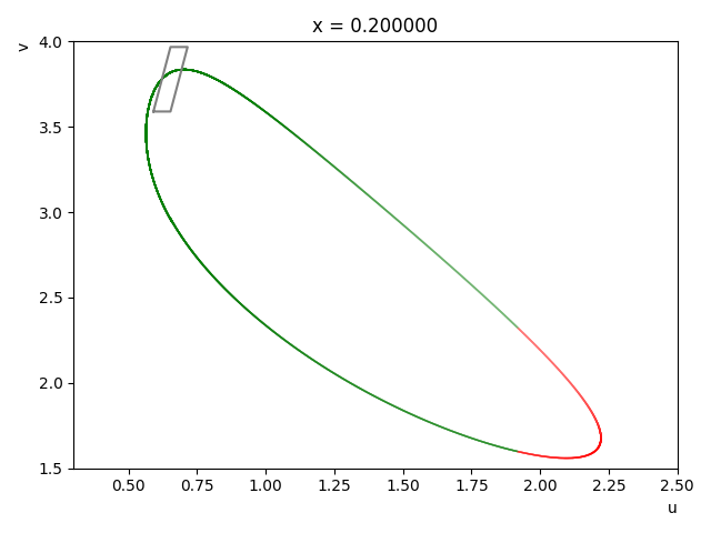
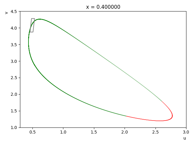
Figure 2: Brusselator: A cyclic trajectory for plan $x=0.2$ (left) and $x=0.4$ (right); the green zone indicates the contractive area ($\lambda<0$) and the red zone the expansive one ($\lambda>0$)

The time-step used in Euler’s method is $\tau=2\cdot 10^{-4}$, and the period of the system is $T=34564\tau$. The expansion factor of the ball radius after one period is $E=2.12$. The number of periods considered for synchronization is $k=5$ (so the expansion factor after $k$ periods $=2.12^{5}\approx 43$). The radius of the balls covering $S$ is $=3.5\cdot 10^{-8}$.

In Fig. 3, we have depicted an initial ball (yellow) with a center of coordinate $(0.622,3.779)$ in plan $x=0.2$, and $(0.486,4.078)$ in plan $x=0.4$; its radius is $3.5\cdot 10^{-8}$. After $k=5$ periods, the image of the yellow ball is the green ball of center $(0.62190185,3.77864437)$ in plan $x=0.2$, and $(0.48594267,4.07798666)$ in plan $x=0.4$; the radius is now $1.5\cdot 10^{-6}$. The phase of the initial ball center is $0.82$ in plan $x=0.2$, and $0.09$ in plan $x=0.4$, so the difference of phase $\Delta(phase(centers))$, at $t=0$, is $0.73$. The phase of the image ball center is $0.87461$ in plan $x=0.2$, and $0.87463$ in plan $x=0.4$, so the difference of phase $\Delta(phase(centers))$, after $k=5$ periods, is now $2\cdot 10^{-5}\approx 0$.

Fig. 4 depicts 10 (pairs of) initial balls with centers located on the parallelepiped perimeters, both in plan $x=0.2$ and $x=0.4$. The coordinates of the 10 (pairs of) centers, given under the form $(u_{1},v_{1},u_{2},v_{2})$, are:

$((0.621890,3.778619,0.485930,4.077929),$ $(0.621895,3.778628,0.485928,4.077933),$

$(0.621889,3.778623,0.485933,4.077953),$ $(0.621902,3.778640,0.485934,4.077946),$

$(0.621892,3.778629,0.485939,4.077966),$ $(0.621886,3.778620,0.485936,4.077966),$

$(0.621895,3.778630,0.485942,4.077978),$ $(0.621900,3.778640,0.485945,4.077991),$

$(0.621905,3.778650,0.485939,4.077978),$ $(0.621902,3.778640,0.485942,4.077990))$

After $k=5$ periods, the coordinates of $(u_{1},v_{1},u_{2},v_{2})$ become $(u^{\prime}_{1},v^{\prime}_{1},u^{\prime}_{2},v^{\prime}_{2})$ as follows:

$((0.621897,3.778636,0.485938,4.077970),$ $(0.621899,3.778639,0.485940,4.077976),$

$(0.621901,3.778643,0.485942,4.077984),$ $(0.621886,3.778617,0.485928,4.077930),$

$(0.621886,3.778617,0.485928,4.077929),$ $(0.621902,3.778645,0.485943,4.077988),$

$(0.621889,3.778623,0.485931,4.077941),$ $(0.621893,3.778629,0.485934,4.077954),$

$(0.621892,3.778627,0.485933,4.077950),$ $(0.621893,3.778629,0.485934,4.077953))$

The two components $(u_{1},v_{1})$ and $(u_{2},v_{2})$ of an initial point, as well as the two components $(u^{\prime}_{1},v^{\prime}_{1})$ and $(u^{\prime}_{2},v^{\prime}_{2})$ of its image, are all the 4 represented with the same color in Fig. 4. The CPU time taken for computing these 10 images is 4,600 seconds (for a program of $PROC1$ in Python running on a 2.80 GHz Intel Core i7-4810MQ CPU with 8 GB of memory.).linecolor=blue,backgroundcolor=blue!25,bordercolor=blue]ÉA: je donnerais un peu plus de détails sur l’implémentation ; et une URL où la trouver ? linecolor=purple,backgroundcolor=purple!25,bordercolor=purple]Jawher: url ajoutée pour les deux applications Table 1 gives the phases of the 10 ball centers shown in Fig. 4. After $k=5$ periods, we have $\Delta(phase(centers))\ll\min(e_{1}/f_{1},e_{2}/f_{2})$, so the difference of phase between the components of a point starting from anywhere in a ball (not necessarily from its center) becomes always $\leq\min(e_{1}/f_{1},e_{2}/f_{2})\approx 0.05$. The proof has been done here for 10 balls, but should be done for the whole set of balls covering $S$. It is easy to see that the number of balls covering $S$ is approximatively $\ell_{1}\ell_{2}E^{4k}/e_{1}e_{2}$, where $\ell_{i}$ is the length of each parallepiped ($i=1,2$). For example, if $\ell_{1}/e_{1}=\ell_{2}/e_{2}=20$, $E^{k}=40$, roughly as in Brusselator, the number of balls is $400\times 40^{4}=2^{10}\cdot 10^{6}\approx 10^{9}$, which is huge. However the analysis can be decomposed into $k$ periods, and accessibility per period proven separately from one intermediate area to the next, thus exponentially decreasing the number of balls. In this case, the procedure has to be performed successively $k$ times, but the number of balls at each time is now just $\ell_{1}\ell_{2}E^{4}/e_{1}e_{2}$, which is $400\times 2^{4}=6400$.

Table 1: The list of phases of 10 ball centers for the Brusselator example.

Phases
Point	phase initial	phase initial	phase image	phase image	$\Delta(phase(centers))$	$\Delta(phase(centers))$
	point in $u_{1}$	point in $u_{2}$	point in $u_{1}$	point in $u_{2}$	for initial point	for image point
1	$0.13$	$0.05$	$0.63224$	$0.63221$	$0.08$	$2\cdot 10^{-}5$
2	$0.40$	$0.10$	$0.72512$	$0.72511$	$0.30$	$8\cdot 10^{-}6$
3	$0.26$	$0.39$	$0.83112$	$0.83113$	$0.13$	$6\cdot 10^{-}6$
4	$0.95$	$0.28$	$0.0383$	$0.0382$	$0.67$	$9\cdot 10^{-}5$
5	$0.42$	$0.57$	$0.0366$	$0.0365$	$0.15$	$9\cdot 10^{-}5$
6	$0.10$	$0.56$	$0.88834$	$0.88836$	$0.46$	$1\cdot 10^{-}5$
7	$0.58$	$0.74$	$0.2103$	$0.2102$	$0.16$	$7\cdot 10^{-}5$
8	$0.66$	$0.92$	$0.3929$	$0.3928$	$0.25$	$5\cdot 10^{-}5$
9	$0.93$	$0.74$	$0.3318$	$0.3317$	$0.19$	$6\cdot 10^{-}5$
10	$0.77$	$0.91$	$0.3890$	$0.3889$	$0.14$	$5\cdot 10^{-}5$

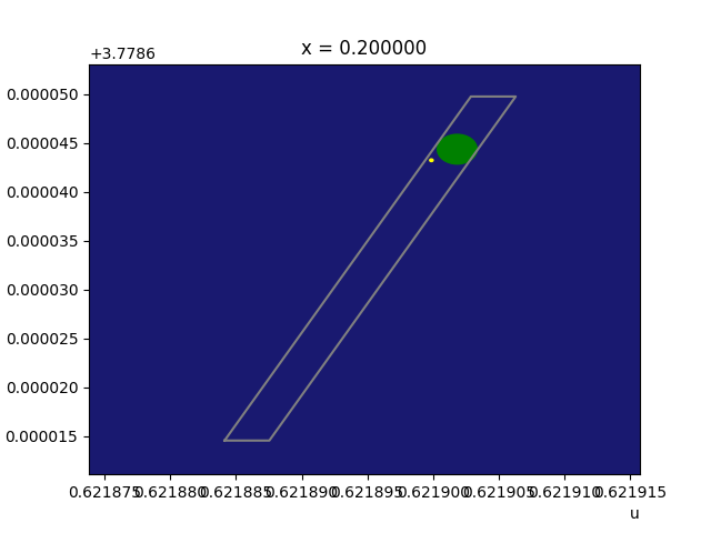
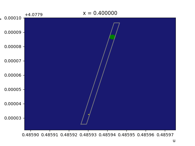
Figure 3: Brusselator: Synchronization of the two components of a ball, located initially near opposite vertices of the parallelograms (yellow), after $k=5$ periods (green).

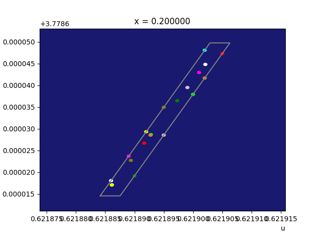
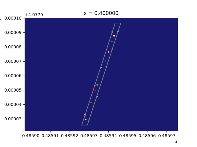
Figure 4: Brusselator: Synchronization of 10 (pairs of) balls, located initially on the parallelogram perimeters, after $k=5$ periods (without radius expansion for clarity).

0.5 Example: Passive biped model

So far, we he have considered only continuous systems governed by ODEs. It is possible to extend the method of verification of phase synchronization to hybrid systems, i. e., continuous systems which, upon the satisfaction of a certain state condition (“guard”), may reset instantaneously the state before resuming the application of ODEs. Many works in the domain of symbolic control have explained how to compute an overapproximation of the intersection of the current set of reachability with the guard condition, and perform the reset operation (see, e. g., [GG08, AK12, KA20]). Our symbolic Euler’s method can be extended along these lines without major problems. We describe here the results of such an extension to the passive biped model [McG90], seen as a hybrid oscillator. The passive biped model exhibits indeed a stable limit-cycle oscillation for appropriate parameter values that corresponds to periodic movements of the legs [SKN17]. The model has a continuous state variable $\textbf{{x}}(t)=(\phi_{1}(t),\overset{.}{\phi_{1}}(t),\phi_{2}(t),\overset{.}{\phi_{2}}(t))^{\top}$. The dynamics is described by $\dot{\textbf{{x}}}=\textbf{{\em f}}(\textbf{{x}})$ with:

$$\textit{{f}}(\textbf{{x}})=\begin{pmatrix}\overset{.}{\phi_{1}}\\ \sin(\phi_{1}-\gamma)\\ \overset{.}{\phi_{2}}\\ \sin(\phi_{1}-\gamma)+\overset{.}{\phi_{1}^{2}}\sin\phi_{2}-\cos(\phi_{1}-\gamma)\sin\phi_{2}\end{pmatrix}$$ (3)

$$Reset(\textbf{{x}})=\begin{pmatrix}-\phi_{1}\\ \overset{.}{\phi_{1}}\sin(2\phi_{1})\\ -2\phi_{1}\\ \overset{.}{\phi_{1}}\cos 2\phi_{1}(1-\cos 2\phi_{1})\end{pmatrix}$$ (4)

$$Guard(\textbf{{x}})\equiv(2\phi_{1}-\phi_{2}=0\ \wedge\phi_{2}<-\delta).$$ (5)

We set $\delta=0.1$ and $\gamma=0.009$. See [McG90] for details. We give in Fig. 5 a typical cyclic trajectory in plans $\phi_{1}$ and $\phi_{2}$, during one period $T$. The coordinates of the parallelepiped vertices are for plan $\phi_{1}$:

$((0.067939,-0.083172),$ $(0.067943,-0.083172),$ $(0.067943,-0.083169),$ $(0.067939,-0.083169))$,

and for plan $\phi_{2}$:

$((0.271972,-0.242725),$ $(0.271983,-0.242734),$ $(0.271983,-0.242731),$ $(0.271972,-0.242722))$.

These parallepipeds are depicted in Fig. 6 (and also at magnified scale in Fig. 5).

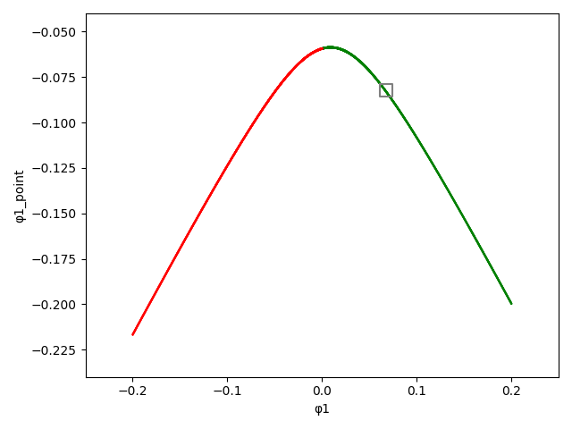
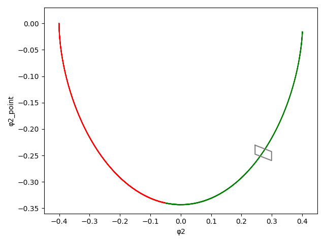
Figure 5: Biped: A cyclic trajectory for plan $\phi_{1}$ (left) and $\phi_{2}$ (right); the green zone indicates the contractive area ($\lambda<0$) and the red zone the expansive one ($\lambda>0$)

The time-step used in Euler’s method is $\tau=2\cdot 10^{-5}$. The period of the system is $T=776440\tau$. The radius expansion factor after one period is $E=2.63$. The number of periods considered for synchronization is $k=30$.

Fig. 6 depicts 10 (pairs of) initial balls with centers located on the parallelepiped perimeters, both in plan $\phi_{1}$ and $\phi_{2}$. The coordinates of these 10 (pairs of) centers, given under the form $(\phi_{1},\overset{.}{\phi_{1}},\phi_{2},\overset{.}{\phi_{2}})$, are:

$((0.067940,-0.083172,0.27198,-0.242729),$ $(0.067942,-0.083168,0.271975,-0.242727),$

$(0.067941,-0.083168,0.271973,-0.242723),$ $(0.067943,-0.0831719,0.271978,-0.242727),$

$(0.067940,-0.0831682,0.271973,-0.242726),$ $(0.067941,-0.0831719,0.271981,-0.242732),$

$(0.067940,-0.0831682,0.271979,-0.242731),$ $(0.067942,-0.0831719,0.271976,-0.242725),$

$(0.067943,-0.0831682,0.271977,-0.242729),$ $(0.067941,-0.0831719,0.271981,-0.242730))$

The coordinates $(\phi^{\prime}_{1},\overset{.}{\phi^{\prime}_{1}},\phi^{\prime}_{2},\overset{.}{\phi^{\prime}_{2}})$ of their images after 30 periods are:

$((0.0679418,-0.0831697,0.271978,-0.242729),$ $(0.0679434,-0.0831707,0.271983,-0.242732),$

$(0.0679425,-0.0831712,0.271982,-0.242732),$ $(0.0679416,-0.0831713,0.271979,-0.242729),$

$(0.0679412,-0.0831698,0.271976,-0.242726),$ $(0.0679408,-0.0831702,0.271976,-0.242726),$

$(0.0679431,-0.0831701,0.271981,-0.242730),$ $(0.0679407,-0.0831703,0.271976,-0.242726),$

$(0.0679426,-0.0831700,0.271980,-0.242729),$ $(0.0679405,-0.0831707,0.271977,-0.242729))$

The two components $(\phi_{1},\dot{\phi}_{1})$ and $(\phi_{2},\dot{\phi}_{2})$ of an initial point, as well as the two components $(\phi^{\prime}_{1},\dot{\phi}^{\prime}_{1})$ and $(\phi^{\prime}_{2},\dot{\phi}^{\prime}_{2})$ of its image, are all the 4 represented with the same color in Fig. 6. The CPU time taken for computing the 10 images is 6,800 secondslinecolor=blue,backgroundcolor=blue!25,bordercolor=blue]ÉA: redire que c’est avec le même programme ? (for a program written in Python running on the same machine used for the Brusselator example). Table 2 gives the phases of the 10 (pairs of) points shown in Fig. 6. After $k=30$ periods, we have $\Delta(phase(centers))\leq 0.25$. Since $\min(e_{1}/f_{1},e_{2}/f_{2})\approx 0.15$, the difference of phase between the components of a point starting anywhere from a ball (not necessarily fom its center), becomes always $\leq 0.4$. Here again, the proof has been done for 10 balls, but should be done for the whole set of balls covering $S$.

Table 2: The list of phases of 10 ball centers in the biped example.

Phases
Point	Phase initial	Phase initial	Phase image	phase image	$\Delta(phase(centers))$	$\Delta(phase(centers))$
	point in $\phi_{1}$	point in $\phi_{2}$	point in $\phi_{1}$	point in $\phi_{2}$	for initial point	for image point
1	0.88	0.29	0.45	0.48	0.59	0.03
2	0.38	0.75	0.05	0.02	0.37	0.03
3	0.55	0.94	0.27	0.07	0.39	0.21
4	0.14	0.48	0.52	0.35	0.34	0.17
5	0.88	0.94	0.62	0.64	0.05	0.03
6	0.55	0.20	0.71	0.65	0.35	0.06
7	0.72	0.39	0.14	0.23	0.33	0.09
8	0.30	0.71	0.74	0.67	0.40	0.07
9	0.22	0.61	0.25	0.32	0.40	0.08
10	0.72	0.16	0.78	0.53	0.56	0.25

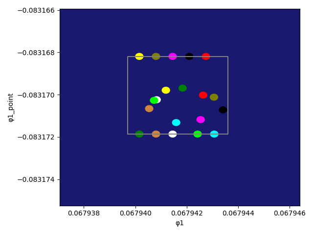
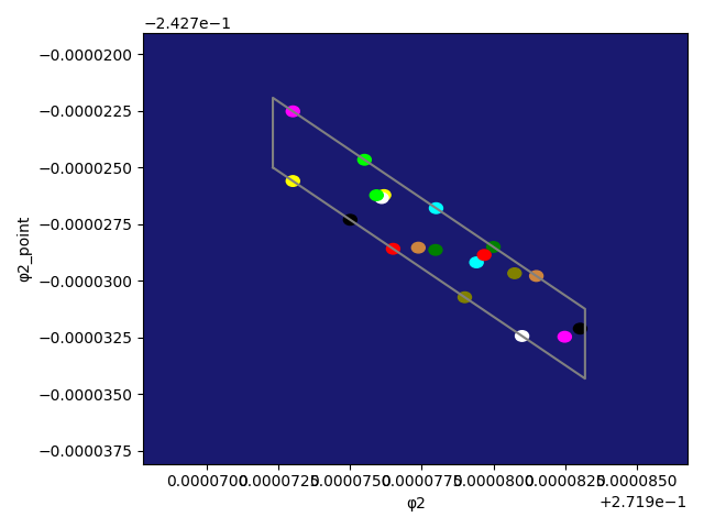
Figure 6: Biped: Synchronization of 10 (pairs of) balls, located initially on the parallelogram perimeters, after $k=30$ periods (without radius expansion for clarity).

0.6 Final Remarks

We have described a symbolic reachability method to prove phase synchronization of oscillators, and illustrated it on the Brusselator and biped examples. The method is inspired by the classical “direct method” which shows that a finite number of points, displaced from their original position on a synchronization orbit, return after some time into a close neighborhood of the orbit. In contrast to the classical method, our symbolic method shows an analogous property for the infinite set $S$ of points located around a portion of the orbit. Such a set $S$ can be determined using simulation methods, but we assume here that it is given. Note that our method guarantees that the solution components are almost synchronized when they pass into $S$, whereas standard synchronization states the stronger property of convergence to the synchronization orbit.

Because of the magnification of the balls on a non-contractive space ($\lambda>0$), one is forced to start with small initial balls, and the coverage of $S$ requires a priori a huge number of balls. However, as explained on the Brusselator example, the analysis can be decomposed into periods, and accessibility per period proven separately from one intermediate area to the next, thus exponentially decreasing the number of balls. Note that the ball magnification problem does not occur on a contractive system ($\lambda<0$), e. g., for Brusselator with a large diffusion coefficient $\sigma$, so the reachability analysis is easier in this case.

We focused here on $n=2$ components with state space dimension $m=2$. The extension to $n,m\geq 3$ is easy in principle, but causes combinatorial explosion of the number of balls covering $S$. In order to solve this “curse of dimensionality”, it would be interesting in future work to adapt the classical “adjoint” method (or phase reduction [SKN17]) rather than the “direct” method used here. Note also that our guaranteed method of phase synchronization can be used with any symbolic reachability procedure other than Euler’s method.

References

- [Ace+05] Juan A. Acebrón et al. “The Kuramoto model: A simple paradigm for synchronization phenomena” In Reviews of Modern Physics 77 American Physical Society, 2005, pp. 137–185 DOI: 10.1103/RevModPhys.77.137
- [AK12] Matthias Althoff and Bruce H. Krogh “Avoiding geometric intersection operations in reachability analysis of hybrid systems” In HSCC Beijing, China: ACM, 2012, pp. 45–54 DOI: 10.1145/2185632.2185643
- [Arc11] Murat Arcak “Certifying spatially uniform behavior in reaction-diffusion PDE and compartmental ODE systems” In Automatica 47.6, 2011, pp. 1219–1229 DOI: 10.1016/j.automatica.2011.01.010
- [AS12] Zahra Aminzare and Eduardo D. Sontag “Logarithmic Lipschitz norms and diffusion-induced instability” In CoRR abs/1208.0326, 2012 arXiv: http://arxiv.org/abs/1208.0326
- [AS14] Zahra Aminzare and Eduardo D. Sontag “Contraction methods for nonlinear systems: A brief introduction and some open problems” In CDC, 2014, pp. 3835–3847 DOI: 10.1109/CDC.2014.7039986
- [CP93] Philippe Chartier and Bernard Philippe “A parallel shooting technique for solving dissipative ODE’s” In Computing 51.3, 1993, pp. 209–236 DOI: 10.1007/BF02238534
- [Fan+17] Chuchu Fan, James Kapinski, Xiaoqing Jin and Sayan Mitra “Simulation-Driven Reachability Using Matrix Measures” In ACM Transactions on Embedded Computing Systems 17.1, 2017, pp. 21:1–21:28 DOI: 10.1145/3126685
- [Fri17] Laurent Fribourg “Euler’s Method Applied to the Control of Switched Systems” In FORMATS 10419, LNCS Berlin, Germany: Springer, 2017, pp. 3–21 DOI: 10.1007/978-3-319-65765-3˙1
- [GG08] Antoine Girard and Colas Le Guernic “Zonotope/Hyperplane Intersection for Hybrid Systems Reachability Analysis” In HSCC 4981, LNCS St. Louis, MO, USA: Springer, 2008, pp. 215–228 DOI: 10.1007/978-3-540-78929-1˙16
- [KA20] Niklas Kochdumper and Matthias Althoff “Reachability Analysis for Hybrid Systems with Nonlinear Guard Sets” In HSCC, 2020, pp. 1:1–1:10 DOI: 10.1145/3365365.3382192
- [KZH02] István Z. Kiss, Yumei Zhai and John L. Hudson “Emerging Coherence in a Population of Chemical Oscillators” In Science 296.5573 American Association for the Advancement of Science, 2002, pp. 1676–1678 DOI: 10.1126/science.1070757
- [Le ̵+17] Adrien Le Coënt, Florian De Vuyst, Ludovic Chamoin and Laurent Fribourg “Control Synthesis of Nonlinear Sampled Switched Systems using Euler’s Method” In SNR 247, EPTCS, 2017, pp. 18–33 DOI: 10.4204/EPTCS.247.2
- [Mag79] Kenjiro Maginu “Stability of spatially homogeneous periodic solutions of reaction-diffusion equations” In Journal of Differential Equations 31 Academic Press, Inc., 1979, pp. 130–138 DOI: 10.1016/0022-0396(79)90156-6
- [McG90] Tad McGeer “Passive Dynamic Walking” In The International Journal of Robotics Research 9.2, 1990, pp. 62–82 DOI: 10.1177/027836499000900206
- [MS90] Renato E. Mirollo and Steven H. Strogatz “Synchronization of Pulse-Coupled Biological Oscillators” In SIAM Journal on Applied Mathematics 50.6 SIAM, 1990, pp. 1645–1662 DOI: 10.1137/0150098
- [RR17] Matthias Rungger and Gunther Reissig “Arbitrarily precise abstractions for optimal controller synthesis” In CDC, 2017, pp. 1761–1768 DOI: 10.1109/CDC.2017.8263904
- [RR19] Gunther Reissig and Matthias Rungger “Symbolic Optimal Control” In IEEE Transactions on Automatic Control 64.6, 2019, pp. 2224–2239 DOI: 10.1109/TAC.2018.2863178
- [Sha+13] S. Shafi, Zahra Aminzare, Murat Arcak and Eduardo D. Sontag “Spatial uniformity in diffusively-coupled systems using weighted L2 norm contractions” In ACC, 2013, pp. 5619–5624 DOI: 10.1109/ACC.2013.6580717
- [SKN17] Sho Shirasaka, Wataru Kurebayashi and Hiroya Nakao “Phase reduction theory for hybrid nonlinear oscillators” In Physical Review E 95 American Physical Society, 2017 DOI: 10.1103/PhysRevE.95.012212
- [Söd06] Gustaf Söderlind “The logarithmic norm. History and modern theory” In BIT Numerical Mathematics 46.3, 2006, pp. 631–652 DOI: 10.1007/s10543-006-0069-9
- [Win80] Arthur T. Winfree “The Geometry of Biological Time” 8, Biomathematics, 1980