Running Head: Spatial occupancy models

Using machine learning to identify nontraditional spatial dependence in occupancy data

Narmadha M. Mohankumar

Department of Statistics, Kansas State University

Trevor J. Hefley

Department of Statistics, Kansas State University

Open Research statement: The Thomson’s gazelle data and sugar glider data used in our data example both are available from the Dryad Digital Repository (Hepler et al. (2019); Stojanovic (2019)): https://doi.org/10.5061/dryad.34kb373 and https://doi.org/10.5061/dryad.xgxd254bt, respectively. A tutorial showing how to implement our statistical model is provided in Appendix S1. Annotated computer code that can be used to reproduce all results and figures associated with the simulation experiment and data examples are provided in Appendix S2, S3, and S4.

Abstract

Spatial models for occupancy data are used to estimate and map the true presence of a species, which may depend on biotic and abiotic factors as well as spatial autocorrelation. Traditionally researchers have accounted for spatial autocorrelation in occupancy data by using a correlated normally distributed site-level random effect, which might be incapable of identifying nontraditional spatial dependence such as discontinuities and abrupt transitions. Machine learning approaches have the potential to identify and model nontraditional spatial dependence, but these approaches do not account for observer errors such as false absences. By combining the flexibility of Bayesian hierarchal modeling and machine learning approaches, we present a general framework to model occupancy data that accounts for both traditional and nontraditional spatial dependence as well as false absences. We demonstrate our framework using six synthetic occupancy data sets and two real data sets. Our results demonstrate how to identify and model both traditional and nontraditional spatial dependence in occupancy data which enables a broader class of spatial occupancy models that can be used to improve predictive accuracy and model adequacy.

Key-words: hierarchical Bayesian model; machine learning; occupancy model; presence–absence data; site occupancy; spatial dependence; zero-inflated binomial model

Introduction

Many ecological studies collect occupancy data to understand the dynamics of species occurrence over space and time (e.g., Hepler et al. 2018; Joseph 2020). Occupancy data are collected by making replicated visits to sites and recording the presence or absence of at least one individual. During a site visit, individuals may go undetected even when present, resulting in the detection of no individuals (i.e., a false absence). Failure to account for false absences can have a significant impact on parameter estimates and predictions (Hoeting et al. 2000; MacKenzie et al. 2002; Tyre et al. 2003).

To facilitate the analysis of occupancy data that contain false absences, Hoeting et al. (2000), MacKenzie et al. (2002), and Tyre et al. (2003) introduced a zero-inflated Bernoulli model that specifies a distribution of the observed data given the true presence at a site. Using familiar notation for Bayesian hierarchical models, the conditional distribution of the data is

$$y_{ij}|z_{i},p_{ij}\sim\left\{\begin{matrix}\text{Bernoulli}(p_{ij})&,z_{i}=1\\ 0&,z_{i}=0\end{matrix}\right.,$$ (1)

where $y_{ij}=1$ denotes the presence and detection of one or more individuals at the $i^{\text{th}}$ site ($i=1,2,...,n$) during the $j^{\text{th}}$ sampling period $(j=1,2,...,J_{i})$ and $y_{ij}=0$ denotes that no individuals were detected. Detection of at least one individual depends on the probability $p_{ij}$. The $z_{i}$ is the true presence ($z_{i}=1$) or absence ($z_{i}=0$) at the $i^{\text{th}}$ site, which is assumed to be constant during all $J_{i}$ sampling periods and modeled as

$$z_{i}|\psi_{i}\sim\text{Bernoulli}(\psi_{i})\;.$$ (2)

In Eq. 2, the probability of true presence, $\psi_{i}$, is modeled using an intercept term and $q$ site-level covariates with the equation

$$g^{-1}(\psi_{i})=\mathbf{x}_{i}^{{}^{\prime}}\boldsymbol{\beta}\;,$$ (3)

where $g^{-1}(\cdot)$ is an appropriate link function (e.g., logit or probit), $\mathbf{x}_{i}\equiv(1,x_{1},x_{2},...,x_{q})^{{}^{\prime}}$, and $\boldsymbol{\beta}\equiv(\beta_{0},\beta_{1},\beta_{2},...,\beta_{q})^{{}^{\prime}}$. Within the vector $\boldsymbol{\beta}$, $\beta_{0}$ is the intercept parameter and $\beta_{1},\beta_{2},...,\beta_{q}$ are regression coefficients.

Since the introduction of the occupancy model in Eqs. 1–3, many extensions were developed to address model inadequacies. For example, to account for spatial dependence Johnson et al. (2013) added a correlated normally distributed site-level effect, $\eta_{i}$ (i.e., $(\eta_{1},\eta_{2},...,\eta_{n})^{{}^{\prime}}\sim\text{N}(\mathbf{0},\boldsymbol{\Sigma})$; see ch. 26 in Hooten and Hefley 2019) to Eq. 3 that resulting in

$$g^{-1}(\psi_{i})=\mathbf{x}_{i}^{{}^{\prime}}\boldsymbol{\beta}+\eta_{i}\;.$$ (4)

The approach by Johnson et al. (2013) has been effective in accounting for occupancy model inadequacies caused by traditional spatial dependence (e.g., Wright et al. 2019), which is assumed to have been generated from a correlated normally distributed random effect that imparts varying levels of smoothness on the spatial process. Discontinuities, abrupt transitions, and other “non-normal” spatial processes are common in ecological data, and the traditional spatial random effect may fail to capture such dynamics (e.g., Hefley et al. 2017). Unfortunately, ecologists lack alternative occupancy model specifications that would allow them to check for and, if needed, model nontraditional spatial dependence.

We demonstrate a framework for occupancy data to identify and model both traditional and nontraditional spatial dependence. Our framework takes a machine learning approach to model the site-level effect in Eq. 4 and can identify both traditional and nontraditional spatial dependence. We illustrate this framework using six synthetic data sets containing traditional and nontraditional spatial dependence and then apply our approach to understand the spatial dynamics of Thomson’s gazelle (Eudorcas thomsonii) in Tanzania and sugar gliders (Petaurus breviceps) in Tasmania.

Materials and Methods

Occupancy data requirements

Our proposed modeling framework builds upon the occupancy model of MacKenzie et al. (2002) and Tyre et al. (2003) and therefore is intended for use with occupancy data that was collected with repeated site visits during which the true presence or absence of individuals at a site does not change. In addition, we require that false negative detections are the only observational error. However, our framework is adaptable to accommodate other types of occupancy data (see “Model extensions” in Appendix S1 for additional detail). For example, our framework can be adapted to account for false presence, which occurs when individuals are not present at a site but are recorded as occurring at a site.

Spatial occupancy model framework

Our proposed framework involves lifting the normal distributional assumption in the spatial component that accounts for the spatial dependence. To accomplish this, we replace the site-level effect in Eq. 4 with

$$g^{-1}(\psi_{i})=\mathbf{x}_{i}^{{}^{\prime}}\boldsymbol{\beta}+f(\mathbf{s}_{i})\;.$$ (5)

Conceptually, this is an important change; the $f(\mathbf{s}_{i})$ is an unknown spatially varying process that is a function, $f(\cdot)$, that depends on the coordinate vector, $\mathbf{s}_{i}$, of the $i^{\text{th}}$ site. The function $f(\cdot)$ is always unknown and is approximated.

This change in perspective is common in the field of machine learning, where the goal is to “learn” or approximate an underlying function using data (see ch. 5 in Hastie et al. 2009). This simple change in Eq. 5 expands the types of model specifications for the spatially varying process, $f(\mathbf{s}_{i})$. For example, regression trees are used to learn about underlying functions that have discontinuities and abrupt transitions, and using regression trees to approximate $f(\mathbf{s}_{i})$ could model nontraditional spatial dependence.

Many approaches from machine learning, such as support vector regression, neural networks, boosted regression trees, and Gaussian processes, could approximate $f(\cdot)$. These approaches have been widely used by ecologists to make predictions and inferences about species distributions from abundance and presence-absence data (e.g., De’ath and Fabricius 2000; Cutler et al. 2007; Elith et al. 2008; Golding and Purse 2016). However, machine learning approaches are not widely used to model occupancy data because of the issues associated with false absences. Furthermore, approximating the spatial dependence within the occupancy model using machine learning approaches requires custom programming and a level of technical knowledge that hinders widespread use. The existing approaches that blend machine learning approaches with occupancy models are approach specific (e.g., Hutchinson et al., 2011; Joseph, 2020), and therefore switching among the different types of approaches to approximate $f(\cdot)$ is a challenge. For example, switching from a neural network to a regression tree to approximate $f(\cdot)$ in Eq. 5 would require extensive retooling of computer code, thus hindering model checking, comparisons, and selection.

Fortunately, Shaby and Fink (2012) developed a model-fitting algorithm based on Markov chain Monte Carlo (MCMC) that enables off-the-shelf software for machine learning approaches, such as those available in R (e.g., rpart(...), svm(...), gam(...)), to be embedded within hierarchical Bayesian models. Once the initial computer code is written for the occupancy model, switching among machine learning approaches to approximate $f(\cdot)$ requires modifying only a few lines of code. Details associated with model fitting are provided in Appendix S1 of the Supplementary Material.

Identifying spatial dependence

To identify the type of spatial dependence and check model adequacy, we use a model selection and model checking approach. First, we use a wide variety of approaches to model spatial dependence and then use a measure of predictive accuracy to determine which approach most accurately models the spatial process. We supplement this predictive approach with a measure of model adequacy (e.g., Wright et al. 2019).

Following Hobbs and Hooten (2015), we measure the predictive accuracy using $-2\times\text{LPPD}$, where LPPD is the log posterior predictive density. The $-2\times\text{LPPD}$ is similar to the information criterion used for model selection but uses out-of-sample data rather than in-sample data (Hooten and Hobbs 2015). As such, $-2\times\text{LPPD}$ and the difference in $-2\times\text{LPPD}$ among models can be interpreted similarly to the information criterion that attempts to approximate $-2\times\text{LPPD}$ using in-sample data (e.g., Watanabe-Akaike information criteria). For example, if model A produced a $-2\times\text{LPPD}$ score less than the $-2\times\text{LPPD}$ score produced by model B, then model A has higher predictive accuracy. As a standard of comparison, we fit an occupancy model that does not account for spatial dependence (i.e., Eq. 3; hereafter nonspatial occupancy model).

In addition, we use Moran’s I correlogram to check model adequacy. Moran’s I has been used to detect traditional spatial dependence in the residuals of fitted occupancy models (Wright et al. 2019). However, if traditional approaches fail to capture spatial dependence, then Moran’s I may identify such inadequacies.

Synthetic data examples

For our synthetic data examples, we show the probability of occupancy in Fig. 1, which includes the three scenarios of nontraditional spatial dependence and the three scenarios of traditional spatial dependence listed below.

1. Spatial dependence that has discontinuities and abrupt transitions generated by a step-wise function (nontraditional; Fig. 1a).

2. Spatial dependence forming a circle with the probability of occupancy being low in the center and smoothly increases towards the edges (nontraditional; Fig. 1b).

3. Spatial dependence defined by a cosine function (nontraditional; Fig. 1c).

4. Normally distributed random effect with a correlation matrix specified by a conditional autoregressive process (traditional; Fig. 1d).

5. Normally distributed random effect with a correlation matrix specified by an exponential covariance function (traditional; Fig. 1e).

6. Normally distributed random effect with a correlation matrix specified by a squared exponential covariance function (traditional; Fig. 1f).

For each scenario, we generate synthetic data using Eqs. 1, 2, and 5 on a unit square study area (i.e., $\mathcal{S=}[0,1]\times[0,1]$). We divided the study area, $\mathcal{S}$, into 900 grid cells (sites). We set the true values for the parameters to $p_{ij}=0.5$ and $\beta_{0}=0$ . We exclude covariates and regression coefficients in our synthetic data so that the spatial process is unobstructed when $\psi_{i}$ is mapped onto $\mathcal{S}$, which aids when visual and numerical comparisons are made among the machine learning approaches. From the 900 grid cells, we consider a random sample of $n=200$ sites as the study area with $J_{i}=3$ visits.

We apply our spatial occupancy modeling framework to the six synthetic data sets and compare the performance of four embedded machine learning approaches, which include regression trees, support vector regression, a low-rank Gaussian process, and a Gaussian Markov random field. The low-rank Gaussian process and Gaussian Markov random field are approaches that model traditional spatial dependence for data sets with a large number of sites and have been used in models for occupancy data (Johnson et al. 2013; Heaton et al. 2019). The regression tree and support vector regression are nontraditional approaches and may be capable of identifying nontraditional types of spatial dependence.

We assess the performance of each approach to identify spatial dependence using $-2\times\text{LPPD}$ calculated at 200 sites that were not used for model fitting (hereafter out-of-sample sites) and by using Moran’s I correlogram. In addition, we visually compare the true probability of occupancy ($\psi_{i}$) to the posterior mean of the probability of occupancy ($\text{E}($$\psi_{i}|\mathbf{y})$; Fig. 2). Details associated with the synthetic data are provided in Appendix S2 of the Supplementary Material.

Thomson’s gazelle data

We illustrate our spatial occupancy modeling framework using a data set from Hepler et al. (2018), who reported the presence and absence of Thomson’s gazelle at 195 sites within Serengeti National Park, Tanzania (Fig. 3a). The sites were sampled using a network of motion-sensitive and thermally activated cameras. Images were classified by participants on the citizen science website Snapshot Serengeti. A site visit consisted of an 8-day period during the year 2012 (e.g., January 1–8, 2012). Each site was visited between 1 and 46 times (the mean number of visits was 29). Following Hepler et al. (2018), $y_{ij}=1$ (from Eq. 1) was recorded if an image of at least one Thomson’s gazelle was captured at the $i^{\text{th}}$ site within the $j^{\text{th}}$ 8-d window. A value of $y_{ij}=0$ was recorded if the site was sampled, but no individuals were observed. Of the 195 sites, 141 had at least one detection. We use 100 randomly selected sites for model fitting and reserve the remaining 95 sites to calculate $-2\times\text{LPPD}$.

Similar to our synthetic data example, we apply our spatial occupancy modeling framework by embedding four machine learning approaches, which include regression trees, support vector regression, a low-rank Gaussian process, and a Gaussian Markov random field. We exclude site-level covariates in our data example to illustrate our approaches ability to model multiple processes that generate spatial dependence (e.g., missing site-level covariates and spatial autocorrelation) and to illustrate the ability of our method to serve as a “spatial interpolator” for occupancy data (i.e., similar to indicator or binomial kriging, but accounting for false absences). However, as with traditional occupancy models, we can easily include site-level covariates into our spatial occupancy models. Details associated with the data example are provided in Appendix S3 of the Supplementary Material.

Sugar glider data

We illustrate our modeling framework using a second data set from Allen et al. (2018), who reported the presence and absence of sugar gliders. The data were collected during four or five site visits made to 100 sites in the Southern Forest region of Tasmania (Fig. 4a). Of the 100 sites, 79 had at least one sugar glider detected. Because this data set has a relatively small number of sites, we used 75 randomly selected sites for model fitting and reserve the remaining 25 sites to calculate $-2\times\text{LPPD}$. We use the same modeling approaches for this example as we did in the Thomson’s gazelle example. Details associated with the data example are provided in Appendix S4 of the Supplementary Material.

Results

Synthetic data examples

In scenario 1, the occupancy model with an embedded regression tree performed best because the other embedded machine learning approaches didn’t capture the abrupt transition created by the step-wise spatial process (Fig. 2). The $-2\times\text{LPPD}$ was $348.5$, $377.2$, $377.5$, and $384.0$ for the embedded regression tree, support vector regression, low-rank Gaussian process, and Gaussian Markov random field, respectively. For comparison, the $-2\times\text{LPPD}$ obtained from the nonspatial occupancy model was 433.1. Similarly, for scenario 1, the comparison of the Moran’s I between the occupancy models suggested that spatial dependence must be accounted for using a regression tree; all other approaches resulted in lingering spatial dependence (see Fig. S6 in Appendix S5).

Detailed results for scenarios 2–6 are presented in Appendix S5 of the Supplementary Material. For example, in scenario 2, the spatial dependence forms a circle with the probability of occupancy being low in the center and smoothly increases towards the edge of the circle (Fig. 1b). For scenario 2, we expected and found that the embedded support vector regression performed best (see Appendix S5). This was expected because this machine learning approach is best suited to learn about smoothly varying deterministic functions. In total, the results from the scenarios clearly demonstrated that if the spatial process is a discontinuous step function, then the approaches used to model traditional spatial dependence are not adequate, and the approaches such as regression trees should be used. If the spatial dependence is traditional, the differences among the approaches are less distinct; nevertheless, in general, support vector regression performs superior for smoothly varying processes (see Appendix S5).

Spatial occupancy dynamics of Thomson’s gazelle

Across the four embedded machine learning approaches, the probability of occupancy at a site ranged from 0.45 to 0.95 (Fig. 3b–3e). Generally, the probability of occupancy was high across the entire study area. However, there was a distinct band running from the southwest to the northeast of the study area where the probability of occupancy was much lower (Fig. 3b–3e).

The measure of predictive accuracy, $-2\times\text{LPPD}$, was $669.4$, $668.8$, $671.0$, and $668.7$ for embedded regression trees, support vector regression, a low-rank Gaussian process, and a Gaussian Markov random field, respectively. For comparison, the $-2\times\text{LPPD}$ obtained from the non-spatial occupancy model was 676.7. Comparison of the Moran’s I between the non-spatial and spatial occupancy models suggested that accounting for spatial dependence improves model adequacy; although, the utility of Moran’s I is questionable because the differences among approaches are trivial, which may be due to the small number of sites (see Fig. S1 in Appendix S3; Carrijo and da Silva 2017). In total, the $-2\times\text{LPPD}$ and Moran’s I suggest that spatial dependence should be accounted for in the model. However, Moran’s I and $-2\times\text{LPPD}$ suggested that the differences among machine learning approaches are less distinct; therefore, it is unclear if the spatial dependence is traditional or nontraditional.

Spatial occupancy dynamics of sugar gliders

For the sugar glider data example, the probability of occupancy at a site ranged from 0.48 to 0.97 (Fig. 4b–4e) across the four embedded machine learning approaches. The probability of occupancy was generally high across the entire study area; however, there was an area in the eastern and southeastern portion of the study area where the probability of occupancy was relatively low (i.e., $\psi_{i}<0.60)$, and there were clear visual differences in the probability of occupancy among the four machine learning approaches (Fig. 4b–4e). The measure of predictive accuracy, $-2\times\text{LPPD}$, was $78.2$, $80.4$, $79.6$, and $78.9$ for embedded regression trees, support vector regression, a low-rank Gaussian process, and a Gaussian Markov random field, respectively. For comparison, the $-2\times\text{LPPD}$ obtained from the non-spatial occupancy model was 80.3. Similar to Thomson’s gazelle example, the comparison of the Moran’s I between the occupancy models suggested that accounting for spatial dependence improves model adequacy (see Fig. S1 in Appendix S4). In total, the $-2\times\text{LPPD}$ and Moran’s I suggest that the spatial process (i.e., $f(\cdot)$ in Eq. 5) is best modeled using a regression tree. Using Moran’s I and $-2\times\text{LPPD}$ as evidence, the results suggested that the spatial dependence is nontraditional.

Discussion

The use of occupancy models has increased rapidly since the early 2000s. Occupancy data are inherently spatial, but unfortunately, only a limited number of approaches existed to model the spatial process (i.e., Hoeting et al. 2000; Johnson et al. 2013). This lack of spatial modeling options for occupancy data is in contrast to species distribution models (SDM) that predict the spatial distribution of a species using statistical and machine learning approaches applied to presence-only, count, and presence-absence data. There is a bewildering number of approaches within the SDM literature that are used to model the spatial process. Unfortunately, many of the SDM approaches do not account for contamination in the response variable (e.g., false absences). Understandably ecologists may feel forced to choose between SDM approaches that do not account for contamination in the response variable (e.g., regression trees) and approaches that do, but with a lack of spatial modeling (e.g., occupancy models).

The crux for ecologists planning to use our framework is to determine which machine learning approaches are likely to capture the spatial process, which will require a level of familiarity with the properties of a wide range of machine learning approaches. We recommend James et al. (2013) for a gentle introduction and Hastie et al. (2009) and Murphy (2012) for more advanced and broad presentations. Within the ecological literature, there are also several excellent guides to machine learning approaches (e.g., De’ath and Fabricius 2000; Cutler et al. 2007; Elith et al. 2008).

Recently, the hierarchical modeling framework commonly used in ecology has been expanded to include some types of machine learning approaches such as neural networks (Wikle 2019; Joseph 2020). Our study builds upon this previous work and expands the types of spatial models ecologists can use for data that fit within the occupancy model framework. Although our work is focused on spatial dependence among the true presence at a site, the approach is easily generalizable. For example, Eq. 5 implies a linear effect of the site-level covariates (i.e., $\mathbf{x}_{i}^{{}^{\prime}}\boldsymbol{\beta}$). Shaby and Fink (2012) show how machine learning approaches can be used to capture nonlinear and unknown relationships between covariates and the probability of occupancy, thus alleviating the linear assumption in Eq. 5. Furthermore, many studies that use occupancy models perform covariate selection using model selection techniques (e.g., Hooten and Hobbs (2015)). While model selection techniques work for a small number of covariates, machine learning approaches may be superior when there are a large number of covariates. Another important generalization is that the machine learning approaches can be embedded to model the probability of detection as a function of predictor variables such as Julian date and observer effort (i.e., similar to the use of cubic splines used by Johnston et al. (2018)). To facilitate these extensions, we explain in Appendix S1 how to generalize our framework for other popular ecological models, which is a direct application of the work by Shaby and Fink (2012).

Acknowledgements

We thank Drs. Staci Hepler, Michael Anderson, and Robert Erhardt for assistance with the Thomson’s gazelle data. We thank Dr. Daniel Fink, an anonymous reviewer, and Dr. Julia Jones for comments that improved our manuscript. Funding for this project was provided by the National Science Foundation via grant DEB 1754491.

Figure legends

Figure 1. Synthetic data examples showing the probability of occupancy ($\psi_{i}$ in Eq. 5) at 900 potential sites (pixels) for six scenarios of traditional and nontraditional spatial dependence. The nontraditional scenarios include spatial dependence having discontinuities and abrupt transitions (panel a), forming a circle (panel b), and defined by a cosine function (panel c). The traditional scenarios include spatial dependence generated from a normally distributed random effect with a correlation matrix specified using a conditional autoregressive process (panel d), an exponential covariance function (panel e), and a squared exponential covariance function (panel f).

Figure 2. The probability of occupancy from scenario 1 of the synthetic data example (panel a) and the posterior mean of the probability of occupancy ($\text{E}(\psi_{i}|\mathbf{y})$)) obtained by fitting spatial occupancy models that included an embedded regression tree (panel b), a support vector regression (panel c), a low-rank Gaussian process (panel d), and a Gaussian Markov random field (panel e). The gray squares in the panel are the locations of the 200 sampled sites used for model fitting.

Figure 3. Thomson’s gazelle data from Hepler et al. (2018) collected at 195 sites within Serengeti National Park, Tanzania (panel a) and the posterior mean of the probability of occupancy ($\text{E}(\psi_{i}|\mathbf{y})$; panels b–e). Panels b–e show $\text{E}(\psi_{i}|\mathbf{y})$ obtained by fitting spatial occupancy models that included an embedded regression tree (panel b), a support vector regression (panel c), a low-rank Gaussian process (panel d), and a Gaussian Markov random field (panel e).

Figure 4. Sugar glider data from Allen et al. (2018) collected at 100 sites in the Southern Forest region of Tasmania and the posterior mean of the probability of occupancy ($\text{E}(\psi_{i}|\mathbf{y})$; panels b–e). Panels b–e show $\text{E}(\psi_{i}|\mathbf{y})$ obtained by fitting spatial occupancy models that included an embedded regression tree (panel b), a support vector regression (panel c), a low-rank Gaussian process (panel d), and a Gaussian Markov random field (panel e).

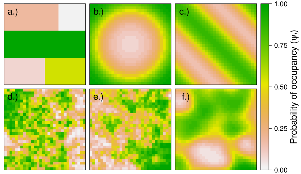
Figure 1:

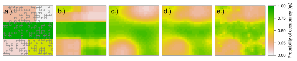
Figure 2:

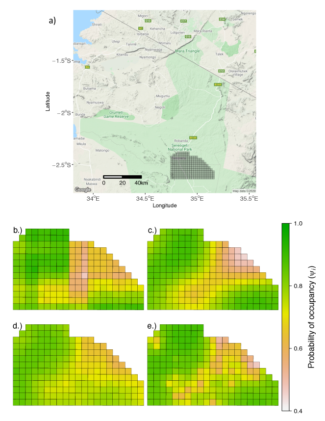
Figure 3:

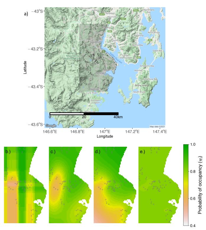
Figure 4:

Literature Cited

- Allen et al. (2018) Allen, M., Webb, M. H., Alves, F., Heinsohn, R., and Stojanovic, D. (2018). Occupancy patterns of the introduced, predatory sugar glider in Tasmanian forests. Austral Ecology, 43(4):470–475.
- Carrijo and da Silva (2017) Carrijo, T. B. and da Silva, A. R. (2017). Modified Moran’s I for small samples. Geographical Analysis, 49(4):451–467.
- Cutler et al. (2007) Cutler, D. R., Edwards Jr, T. C., Beard, K. H., Cutler, A., Hess, K. T., Gibson, J., and Lawler, J. J. (2007). Random forests for classification in ecology. Ecology, 88(11):2783–2792.
- De’ath and Fabricius (2000) De’ath, G. and Fabricius, K. E. (2000). Classification and regression trees: a powerful yet simple technique for ecological data analysis. Ecology, 81(11):3178–3192.
- Elith et al. (2008) Elith, J., Leathwick, J. R., and Hastie, T. (2008). A working guide to boosted regression trees. Journal of Animal Ecology, 77(4):802–813.
- Golding and Purse (2016) Golding, N. and Purse, B. V. (2016). Fast and flexible bayesian species distribution modelling using gaussian processes. Methods in Ecology and Evolution, 7(5):598–608.
- Hastie et al. (2009) Hastie, T., Tibshirani, R., and Friedman, J. (2009). The elements of statistical learning: data mining, inference, and prediction. Springer Science & Business Media.
- Heaton et al. (2019) Heaton, M. J., Datta, A., Finley, A. O., Furrer, R., Guinness, J., Guhaniyogi, R., Gerber, F., Gramacy, R. B., Hammerling, D., Katzfuss, M., et al. (2019). A case study competition among methods for analyzing large spatial data. Journal of Agricultural, Biological and Environmental Statistics, 24(3):398–425.
- Hefley et al. (2017) Hefley, T. J., Hooten, M. B., Hanks, E. M., Russell, R. E., and Walsh, D. P. (2017). Dynamic spatio-temporal models for spatial data. Spatial Statistics, 20:206–220.
- Hepler et al. (2018) Hepler, S. A., Erhardt, R., and Anderson, T. M. (2018). Identifying drivers of spatial variation in occupancy with limited replication camera trap data. Ecology, 99(10):2152–2158.
- Hepler et al. (2019) Hepler, S. A., Erhardt, R., and Anderson, T. M. (2019). Data from: Identifying drivers of spatial variation in occupancy with limited replication camera trap data, dryad, dataset. https://doi.org/10.5061/dryad.34kb373.
- Hobbs and Hooten (2015) Hobbs, N. T. and Hooten, M. B. (2015). Bayesian models: a statistical primer for ecologists. Princeton University Press.
- Hoeting et al. (2000) Hoeting, J. A., Leecaster, M., and Bowden, D. (2000). An improved model for spatially correlated binary responses. Journal of Agricultural, Biological, and Environmental Statistics, 5(1):102–114.
- Hooten and Hefley (2019) Hooten, M. B. and Hefley, T. J. (2019). Bringing Bayesian models to life. CRC Press.
- Hooten and Hobbs (2015) Hooten, M. B. and Hobbs, N. T. (2015). A guide to Bayesian model selection for ecologists. Ecological Monographs, 85(1):3–28.
- Hutchinson et al. (2011) Hutchinson, R. A., Liu, L.-P., and Dietterich, T. G. (2011). Incorporating boosted regression trees into ecological latent variable models. In AAAI, volume 11, pages 1343–1348.
- James et al. (2013) James, G., Witten, D., Hastie, T., and Tibshirani, R. (2013). An introduction to statistical learning. Springer.
- Johnson et al. (2013) Johnson, D. S., Conn, P. B., Hooten, M. B., Ray, J. C., and Pond, B. A. (2013). Spatial occupancy models for large data sets. Ecology, 94(4):801–808.
- Johnston et al. (2018) Johnston, A., Fink, D., Hochachka, W. M., and Kelling, S. (2018). Estimates of observer expertise improve species distributions from citizen science data. Methods in Ecology and Evolution, 9(1):88–97.
- Joseph (2020) Joseph, M. B. (2020). Neural hierarchical models of ecological populations. Ecology Letters, 23(4):734–747.
- MacKenzie et al. (2002) MacKenzie, D. I., Nichols, J. D., Lachman, G. B., Droege, S., Andrew Royle, J., and Langtimm, C. A. (2002). Estimating site occupancy rates when detection probabilities are less than one. Ecology, 83(8):2248–2255.
- Murphy (2012) Murphy, K. P. (2012). Machine learning: a probabilistic perspective. MIT press.
- Shaby and Fink (2012) Shaby, B. A. and Fink, D. (2012). Embedding black-box regression techniques into hierarchical Bayesian models. Journal of Statistical Computation and Simulation, 82(12):1753–1766.
- Stojanovic (2019) Stojanovic, D. (2019). Occupancy patterns of the introduced, predatory sugar glider in tasmanian forests, dryad, dataset. https://doi.org/10.5061/dryad.xgxd254bt.
- Tyre et al. (2003) Tyre, A. J., Tenhumberg, B., Field, S. A., Niejalke, D., Parris, K., and Possingham, H. P. (2003). Improving precision and reducing bias in biological surveys: estimating false-negative error rates. Ecological Applications, 13(6):1790–1801.
- Wikle (2019) Wikle, C. K. (2019). Comparison of deep neural networks and deep hierarchical models for spatio-temporal data. Journal of Agricultural, Biological and Environmental Statistics, 24(2):175–203.
- Wright et al. (2019) Wright, W. J., Irvine, K. M., and Higgs, M. D. (2019). Identifying occupancy model inadequacies: can residuals separately assess detection and presence? Ecology, 100(6):e02703.