Using Wavelets and Spectral Methods to Study Patterns in Image-Classification Datasets

Abstract

Deep learning models extract, before a final classification layer, features or patterns which are key for their unprecedented advantageous performance. However, the process of complex nonlinear feature extraction is not well understood, a major reason why interpretation, adversarial robustness, and generalization of deep neural nets are all open research problems. In this paper, we use wavelet transformation and spectral methods to analyze the contents of image classification datasets, extract specific patterns from the datasets and find the associations between patterns and classes. We show that each image can be written as the summation of a finite number of rank-1 patterns in the wavelet space, providing a low rank approximation that captures the structures and patterns essential for learning. Regarding the studies on memorization vs learning, our results clearly reveal disassociation of patterns from classes, when images are randomly labeled. Our method can be used as a pattern recognition approach to understand and interpret learnability of these datasets. It may also be used for gaining insights about the features and patterns that deep classifiers learn from the datasets.

1 Introduction

Deep learning image classifiers are complex and nonlinear mathematical functions that extract features from images and learn to classify them based on those features. Yet, this mathematical process is not well understood, a major reason why interpretation, adversarial robustness, and generalization of them are all open research problems. By bringing computational methods from the image processing literature, in tandem with spectral methods from the numerical analysis literature, here, we develop computational methods to study the contents of image-classification datasets with the aim to understand the fine level patterns and features of images with respect to classification.

Deep learning functions are formed during training, by the contents of their training sets. Understanding the learning process and generalization, for some data types, may start with direct analysis of the data itself (Bahri et al., 2020). However, studying the contents of image-classification datasets is not straightforward (Strang, 2019), because of the typical difficulties in working with visual signals.

In practice and in research, learning of images is left to the models. From the adversarial point of view, image-classification models are vulnerable and this vulnerability seems inevitable (Shafahi et al., 2019) and even at odds with achieving good accuracy (Tsipras et al., 2019; Ilyas et al., 2019). From the generalization point of view, models are highly over-parameterized and they can fit the contents of their training sets, even when training images are labeled randomly and even if the contents of images get replaced with random noise (Zhang et al., 2017). Recent studies have pursued this dilemma by making the distinction between the concepts of learning vs memorization (Belkin et al., 2018, 2019).

This lack of understanding about the models can partly be explained by our lack of knowledge about fine-grained details of image-classification datasets. Recently, a new line of research has focused on the contents of these datasets, studied the procedures used to gather and label the images, and raised questions about the learning, statistical bias and possible over-fitting of deep classifiers (Recht et al., 2019; Yadav and Bottou, 2019; Recht et al., 2018; Engstrom et al., 2020). Still, there is a need for specialized computational procedures to analyze these datasets and explain what can make one image associated with one class and not with other classes. What is the essence of each image when it comes to classification?

From the optimization perspective, there are infinite number of global minimizers for training loss of image classification models, many of which would perform very badly on testing data (Arora et al., 2019; Neyshabur et al., 2019). Studies that focus on training, aim to find the minimizer that performs well on the testing set. But, the way to confirm that one has chosen a good minimizer of training loss is to measure its accuracy on a testing or validation set, and there is not an independent procedure to investigate whether there are specific associations between patterns and classes. Clearly, we would not expect a randomly labeled training set to have such association and that is why when one achieves zero training loss on such data, we consider it memorization and not learning.

Of course, a human can look at randomly labeled images and confirm the randomness of labels. But, can we devise computational procedures to evaluate that, without using a testing set? We would like such computational procedure to provide us with information such as:

.4cm1 1. There are no specific patterns in a dataset, if content of images are random noise.

2. There are patterns in a dataset but not associated with classes, if images are randomly labeled.

3. There are patterns in a dataset and each class is associated with certain patterns, if images are legitimately labeled and there are patterns in the dataset exclusive to individual classes.

We develop a method to analyze image-classification datasets and provide the information above. Our approach can be considered a pattern recognition method which can analyze the datasets and provide insights about their learnability. We show that each image can be written as the summation of a finite number of rank-1 patterns in the wavelet space; and the main distinguishable patterns in each image can be reconstructed using a relatively small number of those patterns, providing a low-rank approximation to each image. We extract the patterns by tensor decomposition of datasets in the wavelet space and then transform the patterns back to the pixel space. We see that when datasets are randomly labeled, some patterns may emerge but they cannot be associated with specific classes.

2 Using wavelets to extract features from images

Background.

Wavelets are a class of functions and one of the most capable tools to systematically process images and extract features and patterns from them. The difficulty of working with images and many signals arises from the spatial complexity of patterns and structures in them. What makes an image to represent a dog, and not an automobile, cannot be explained by one or even a few pixels, rather, it may be explained by the specific patterns that appear in various regions of an image, and how these different regions are arranged.

Connection of wavelets with deep learning.

In recent years, we have seen the outstanding performance of deep learning models as an image processing tool that can analyze images and learn to classify them. The features learned by these models are sometimes referred to as deep features (Noh et al., 2017; Romero et al., 2015; Chen et al., 2016; Effland et al., 2019). Some studies use deep nets to learn specific features in images, e.g., facial attributes (Hand, 2018; Thom and Hand, 2020). However, the process of complex nonlinear feature extraction by the models is not well understood. This is the gap we want to bridge: to bring tools from the image processing literature and use them in tandem with spectral methods to analyze the contents of image classification datasets.

We note that wavelets have a similar computational nature as the deep learning models. Wavelets decompose an image by convolving a wavelet basis with the image. Deep learning models also rely on convolutional layers that convolve images with stencils/filters. So, our approach of transforming images with wavelets, and then studying their patterns coincides with the approach used by the classification models. Recently, Yousefzadeh (2020) proposed a method that clusters images based on their wavelet coefficients in order to analyze the similarities in image classification datasets, and showed that wavelets identify similar images, the same way that a pre-trained ResNet model does (Birodkar et al., 2019). Also, Bruna et al. (2016) have used wavelets to initialize the filters of convolutional neural nets.

Properties and notation.

There are older forms of data transformation, for example, the Fourier transform which has a long history and widespread applications. In fact, wavelets were developed building on the scientific knowledge of Fourier transform in the context of image and signal processing. For example, Daubechies (1990) showed that wavelets perform better than windowed Fourier transform on visual signals, because wavelets handle the frequencies in a nonlinear way. The family of Daubechies wavelets (Daubechies, 1992) are one of the most successful types of wavelet transformation, and we use them in this paper.

The orthogonality of Daubechies wavelets is particularly useful for feature extraction, because orthogonality in this setting implies the filters are independent and each filter is measuring a specific feature in the image signals. To process images with wavelets, we use the function

$$[\omega,\beta]=wavedec(x,\Omega,N),$$ (1)

which takes as input an image $x$, a wavelet basis $\Omega$, and level number $N$. It returns a vector of real numbers $\omega$, representing the wavelet coefficients obtained from convolving $x$ with $\Omega$, and a book keeping matrix $\beta$ containing the dimensions of wavelet coefficients by level. This operation is reversible, therefore, given $\omega$, $\beta$, and $\Omega$, we can return to pixel space and reconstruct the image $x$, which we denote its operation by

$$x=waverec(\omega,\beta,\Omega).$$ (2)

For a given $N$, $\beta$ will be constant for all images of the same size.

3 Using spectral decomposition to understand the patterns in image datasets

Background.

In general spectral methods are widely used in supervised and unsupervised learning, for example, for manifold learning (Belkin et al., 2006), dictionary learning (Huang and Anandkumar, 2015), and biomedical data (Alter et al., 2000, 2003; Perros et al., 2019). In deep learning, spectral methods are used for compressing the models (Arora et al., 2018; Li et al., 2020), and also for their training (Sedghi et al., 2019). These studies, however, concern the trainable parameters, not the data.

In fact, spectral methods are rarely used on the contents of image classification datasets. An early use of spectral decomposition for image classification is by Savas and Eldén (2007). Their method performs higher order singular value decomposition (De Lathauwer et al., 2000) on pixels of MNIST and uses the decomposition of training set to classify images in the testing set. They apply their method directly to pixels, achieving about 94% testing accuracy. Other examples of using tensor decomposition directly work on image pixels, too. For example, Fang et al. (2017) proposed a tensor based compression method for on-ground spectral imaging. Ali and Foroosh (2016) used tensor decomposition for character recognition. Applying tensor decomposition directly on image pixels might be able to extract some usable patterns, if images contain simple patterns like word characters. However, as we explained earlier, extracting sophisticated patterns from images requires more advanced tools, such as wavelets.

Higher Order GSVD.

Higher Order Generalized Singular Value Decomposition (HO-GSVD) is viewed under the broad category of Tucker tensor decomposition methods (Kolda and Bader, 2009). Originally developed by Van Loan (1976), it was advanced to the higher order case (Omberg et al., 2007; Ponnapalli et al., 2011), where $n$ number of (full column rank) matrices, $\mathcal{D}_{i},i\in\{1,2,\dots,n\}$, can be decomposed as

$$\mathcal{D}_{i}=U_{i}\Sigma_{i}V,\;\forall i\in\{1,2,\dots,n\},$$ (3)

where, $U_{i}$’s, are composed of normalized left basis vectors, the singular values are positive scalars organized in diagonal elements of $\Sigma_{i}$, and the normalized orthogonal right basis $V$ is common among all the $n$ decompositions. It is proved that the resulting decomposition extends all of the mathematical properties of the GSVD, except for orthogonality of the columns of left basis vectors (Ponnapalli et al., 2011; Alter, 2018).

The vectors in $V$ can generally be viewed as the patterns present in all $\mathcal{D}_{i}$’s. The singular values are the key to understand which pattern is specific to each class and which patterns are shared among classes. For example, if the $j$th singular value of $\Sigma_{i}$ is significantly larger (dominant) than the $j$th singular values for all other classes, it means that the $j$th vector in $V$ is specific to the class $i$. We expand further on this kind of interpretation in our numerical results. Additionally, we can use this decomposition to write each $\mathcal{D}_{i}$ as the summation of $m$ rank-1 matrices.

$$\mathcal{D}_{i}=\sum_{j=1}^{m}\sigma_{j}U_{i}(:,j)V_{i}(j,:)$$ (4)

Other methods.

Using other forms of tensor decomposition may be useful, too. In particular Canonical Polyadic Decomposition can be useful for certain aspects of our analysis, because it breaks the data into rank-1 components (patterns), and the number of components corresponds to the rank of tensor. Recently, Hong et al. (2020) presented an algorithm for generalized canonical polyadic (GCP) low-rank tensor decomposition, which we plan to explore in future research.

Choosing a subset of influential wavelet coefficients.

The HO-GSVD has stable and efficient numerical algorithms for its computation and there are well-studied theoretical properties about it. But in order to benefit from such algorithms and mathematical properties, the individual matrices for each class should have full column rank. Some datasets may naturally satisfy such property, as we see for CIFAR-10 dataset. But, this is not satisfied for some other datasets, for example MNIST and Omniglot. In order to choose a subset of most influential wavelet coefficients, satisfying the full column rank requirement, we use rank-revealing QR factorization (RR-QR) (Chan, 1987). This method orders the columns of a matrix based on their rank influence. Hence, we can easily choose a subset of most influential coefficients satisfying the full column rank. This approach of using rank-revealing QR factorization to choose a subset of wavelet coefficients is previously suggested by Yousefzadeh and O’Leary (2020).

4 Formal procedure

Our approach.

The main goal, here, is to extract features and patterns from image-classification dataset, $\mathcal{P}$, and find the association of patterns to classes. Our algorithm first transforms the images into a wavelet space, organizes them into a tensor $\mathcal{D}$, analyzes the tensor and removes its redundancies and rank deficiencies, performs spectral decomposition on $\mathcal{D}$, analyzes the decomposition, and finally, reconstructs the patterns back in the pixel space, and provides low-rank approximation for images.

Our algorithm.

We now formalize our procedure in Algorithm 1. Line 1 counts the number of classes, $n_{c}$. Line 2 through 7 decomposes all images using wavelet basis $\Omega$ and organize them in a rank-3 tensor, where each $\mathcal{D}_{i}$ represents each class, rows of each $\mathcal{D}_{i}$ represent the $n_{i}$ images in that class and its columns represent the $m$ wavelet coefficients of images. We discuss the choice of wavelet basis for our numerical experiments in Appendix A. Note that the slices of $\mathcal{D}$ have different number of images and HO-GSVD can decompose such tensor.

Algorithm 1 Wavelets Spectral Decomposition for Pattern Association (WSDPA): Algorithm for analyzing the patterns in image-classification datasets using wavelets and spectral decomposition

Inputs: Dataset $\mathcal{P}$ (in pixel space), wavelet basis $\Omega$, $\tau$, tensor decomposition method $\mathcal{M}$
Outputs: Reconstructed patterns in pixel space $\nu_{k}$ and their association to each class, Decomposition of $\mathcal{D}$

1:  Count total number of classes in $\mathcal{P}$ as $c$

2:  for $i=1$ to $c$ do

3:     $n_{i}=$ total number of images in class $i$

4:     for $j=1$ to $n_{i}$ do

5:        $\mathcal{D}(j,:,i)=wavedec(P\{i\}\{j\},\Omega)$

6:     end for

7:  end for

8:  $\alpha=mean(\mathcal{D},``all")$, $m=$ number of wavelet coefficients per image

9:  $S_{n,c}=\mathcal{D}_{n,m,c}\times_{m}\mathbbm{1}_{m,1}$

10:  $\forall{(i\in\{1,\dots,c\},j\in\{1,\dots,n_{i}\})}\rightarrow\mathcal{D}(j,:,i)=\mathcal{D}(j,:,i)\odot(\alpha/S(j,i))$

11:  if $m\leq$ total number of images in $\mathcal{P}$ then

12:     Stack all $\mathcal{D}(:,:,i),\forall{i\in\{1,\dots,c\}}$ into a single matrix $A$ and perform rank-revealing QR factorization to obtain $PA=QR$

13:     for $i=1$ to $n_{c}$ do

14:        $\hat{\gamma}_{i}=\min\big{(}n_{i},\arg\max\limits_{\gamma}\kappa\big{(}P(1:\gamma,:)\mathcal{D}_{i}\big{)}\leq\tau\big{)}$

15:     end for

16:     $m=\min(\hat{\gamma}_{i},i\in\{1,\dots,c\})$

17:     $\forall(i\in\{1,\dots,c\})\rightarrow\mathcal{D}_{i}=P(1:m,:)\;\mathcal{D}_{i}$

18:  else

19:     Warning: “Samples are fewer than features."

20:  end if

21:  Perform spectral decomposition on rank-3 tensor $\mathcal{D}$ using method $\mathcal{M}$$\rightarrow$ e.g., using HO-GSVD: $\mathcal{D}=U_{i}\Sigma_{i}V,\forall{i\in\{1,\dots,c\}}$

22:  Analyze the patterns in decomposition, reconstruct them, and find their association to classes $\rightarrow$ $\nu_{k}=waverec(V(:,k),\Omega)$ to reconstruct the patterns in pixel space$\rightarrow$ Find association of $\nu_{k}$’s to each class based on singular values

23:  return the decomposition and patterns

Line 8 computes the total average of all the wavelet coefficients in $\mathcal{D}$ and defines $m$ as the number of wavelet coefficients per image. Line 9 sums the values of $\mathcal{D}$ over the dimension of wavelet coefficients, to obtain $S$, and line 10 scales the wavelet coefficients for each image, so that the sum of wavelet coefficients becomes equal for all images. Lines 11 through 20 are about choosing the most influential wavelet coefficients. Such feature selection requires the total number of images in the dataset to be more than the number of wavelet coefficients per image. This is naturally satisfied in some image classification datasets, but in cases where it is not satisfied, one can reduce the resolution of images, before feeding them to Algorithm 1. Further discussion is provided in Appendix C.

Line 12 performs RR-QR algorithm on all the data to sort the wavelet coefficients based on their importance (linear independency). Lines 13 through 15 loop over slices of the tensor and find the maximum number of wavelet coefficients that can be used while satisfying the conditions discussed in Section 3. $\kappa(.)$ computes the 2-norm condition number. Line 16, chooses $m$ as the number of coefficients that satisfy the requirements for all slices of $\mathcal{D}$. Line 17 keeps the $m$ most influential wavelet coefficients and discards the rest of coefficients for all images. In choosing the $m$, Algorithm 1 uses a parameter $\tau$ which is an upper limit on the condition number of slices of the tensor corresponding to each class. Finally, Lines 21 and 22 perform the spectral decomposition on $\mathcal{D}$ and analyzes the patterns in the decomposition. This process involves reconstructing the patterns in the pixel space. Based on the spectral method used, we can find the association of patterns to classes, by identifying which patterns are almost exclusively contributing to specific classes.

5 Numerical Experiments

Here, we study the patterns in CIFAR-10 (Krizhevsky, 2009). Our results on MNIST (LeCun et al., 1998) are presented in Appendix D. We first consider two classes of Cat and Dog in the CIFAR-10, because they are two of the most similar classes and make up most of the mistakes by the state of art model (Kolesnikov et al., 2019). To decompose images, we use the Daubechies-2 wavelet basis. In Appendix A, we explain the reason for this choice. The number of wavelet coefficients we use is $m=3,000$ in this example, which corresponds to using $\tau=7\times 10^{4}$ in Algorithm 1.

Singular values reveal patterns specific to each class. Each $D_{i}$ has its own set of singular values, $\Sigma_{i}$. Comparison of singular values in $\Sigma_{1}$ and $\Sigma_{2}$ reveals which patterns (i.e., vectors in $V$) are influential for cats and which patterns are influential for dogs. Figure 1 shows the first 400 singular values for cats and dogs. The ratio of singular values and also the angular distance between them can be insightful in this analysis, as suggested by Bradley et al. (2019). When two singular values are equal for a particular basis, it means that the basis is equally common for them and not discriminative. But, when a singular value for one class is much larger compared to other classes, it means that the corresponding basis in $V$ is specific to that class. In Figure 1, we can see many such cases.

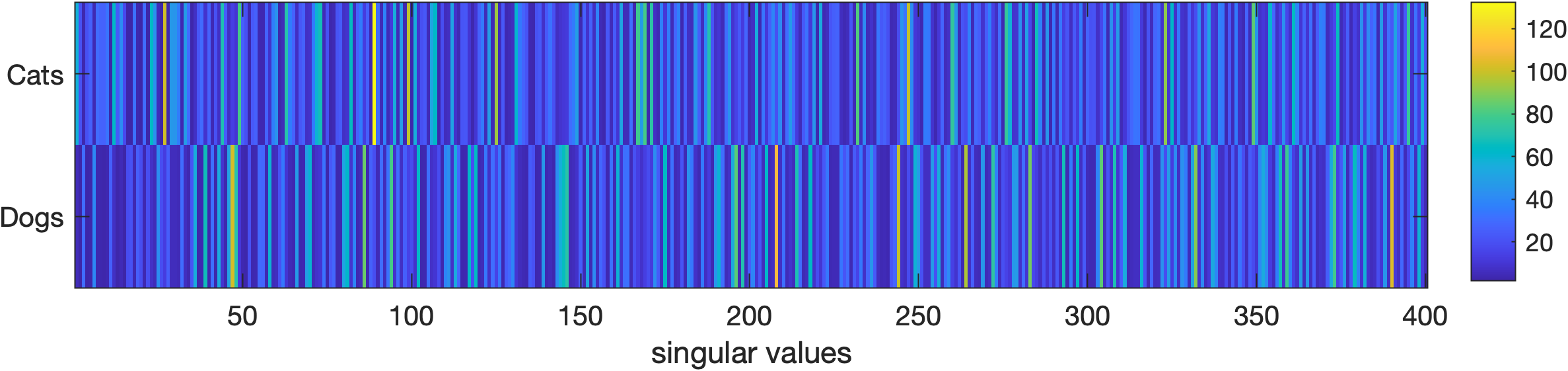
Figure 1: The first 400 singular values of $\Sigma_{1}$ and $\Sigma_{2}$. Larger singular value for one class signifies the importance of corresponding right basis for that class. Clearly, there are distinct separations between some of the singular values.

Reconstructing the patterns back in the pixel space. Each column in $V$ corresponds to a pattern and we can reconstruct the patterns back in the pixel space, using the same wavelet basis. Figure 2(a) shows the four most dominant bases for Dogs, in the pixel space. By dominant, we mean these bases have large singular values for the Dog class, but small singular values for Cats. Similarly, Figure 2(b) shows the patterns dominant for cats, back in the pixel space.

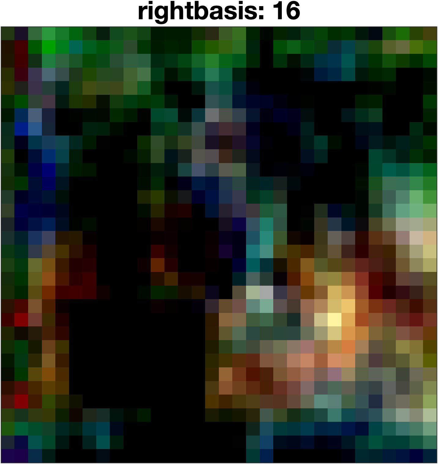
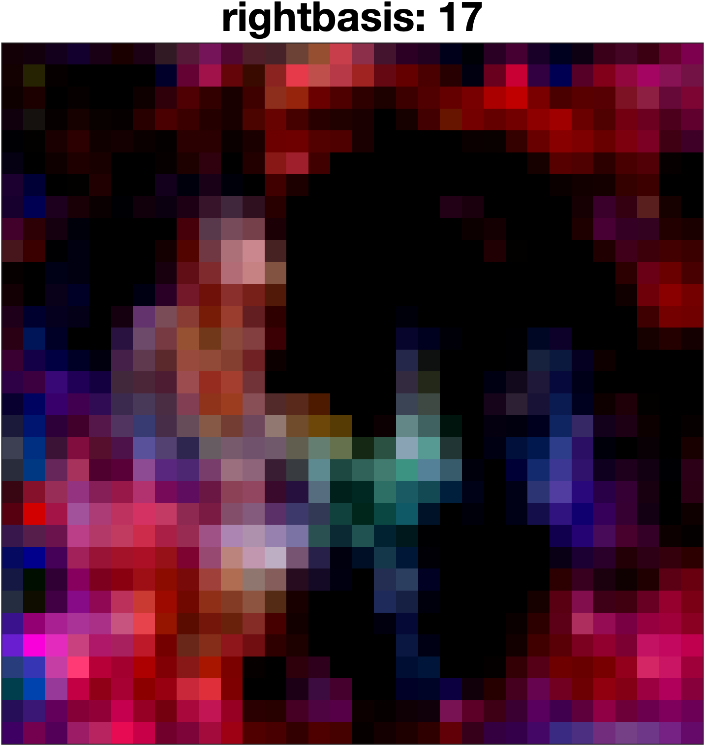
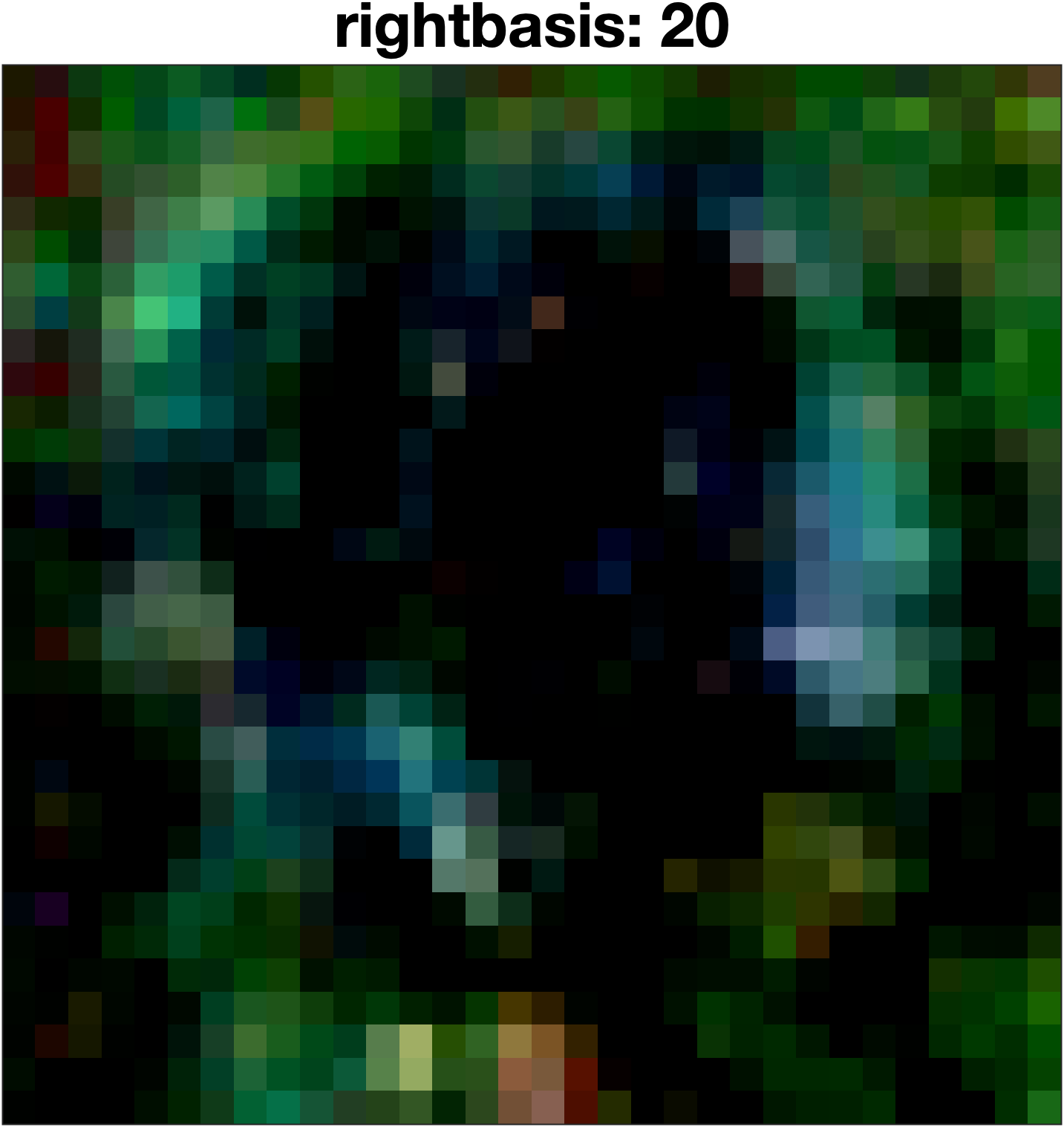
(a) Dogs.

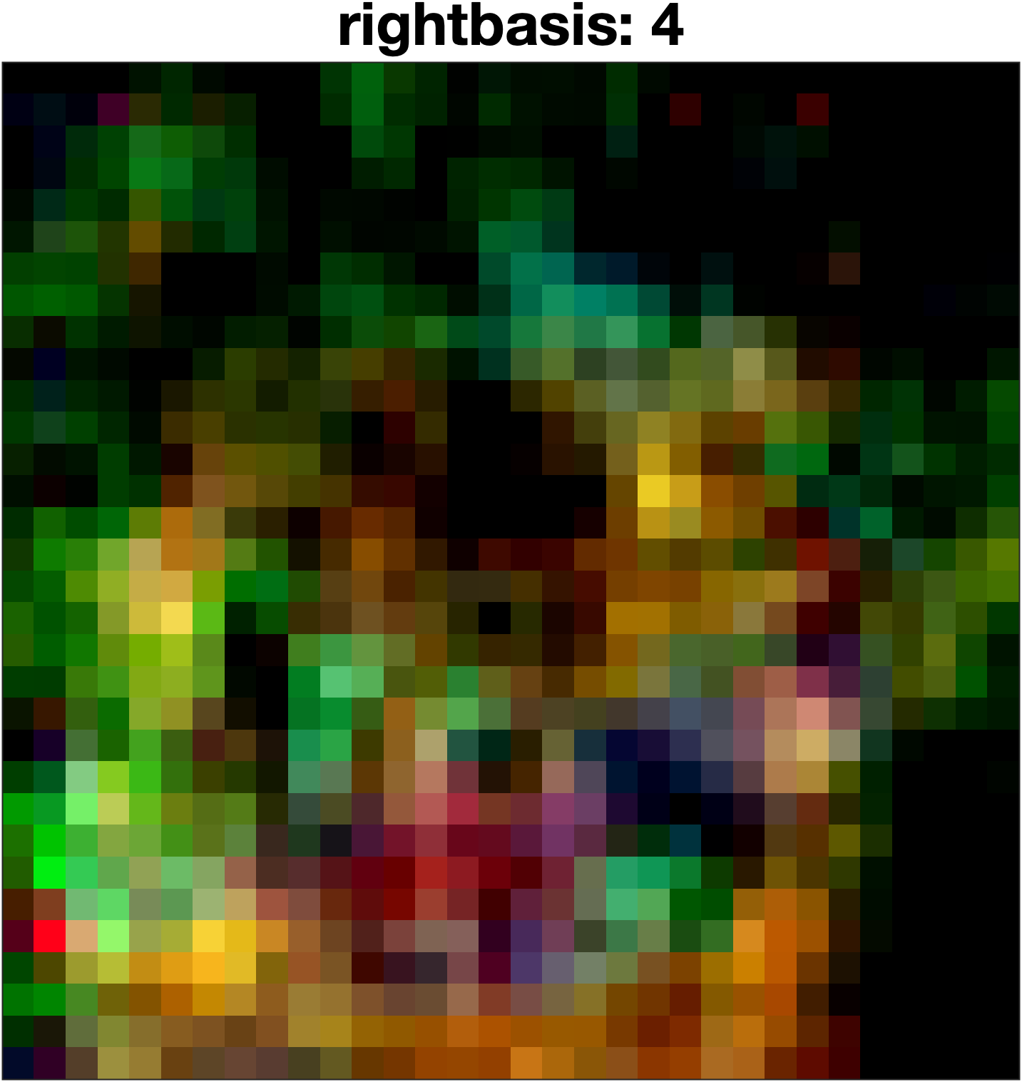
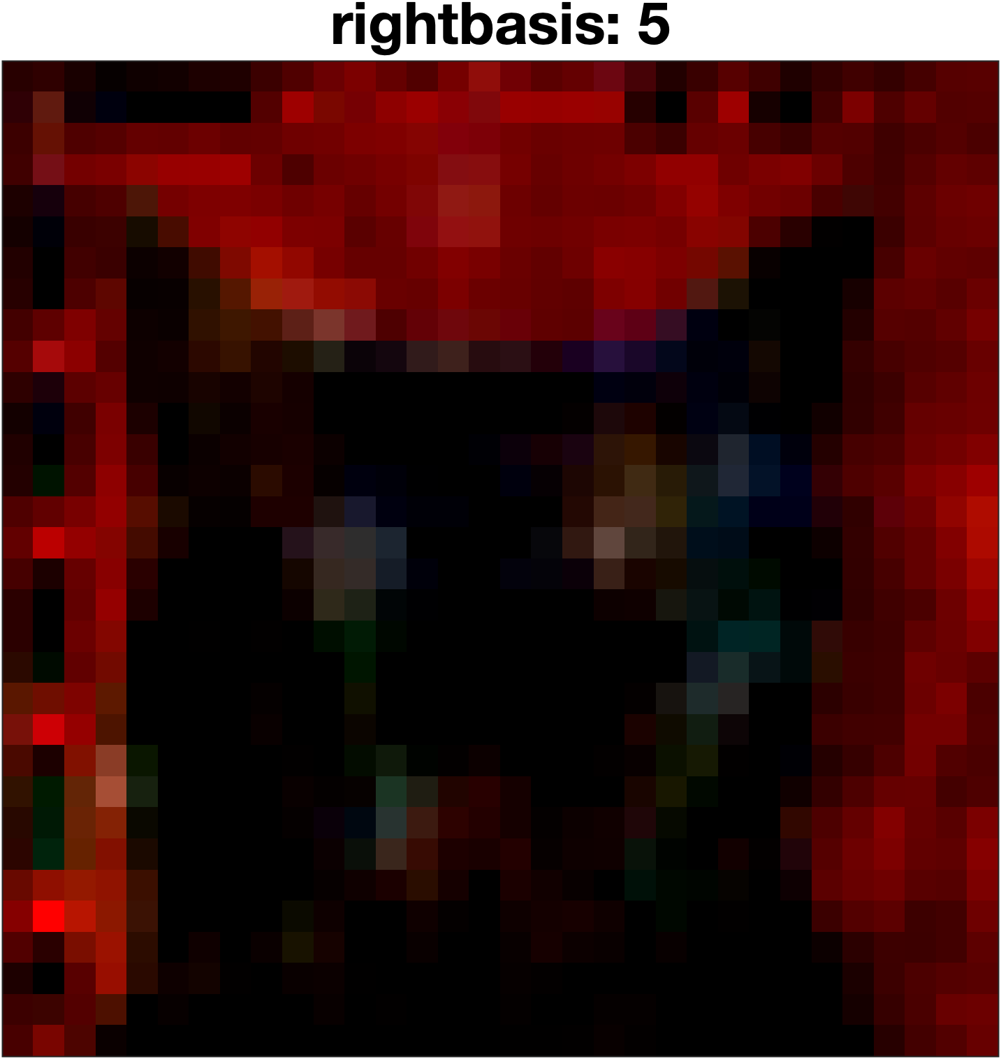
(b) Cats.

Figure 2: Images reconstructed in the pixel space from the most dominant right basis columns.

Understanding the contribution of each pattern to each image. Each of the patterns present in $V$ contribute to each image in the dataset with some coefficient, determined in the left basis. In fact, we can write each image as the summation of the patterns in the pixel space, using Equation 4. Figure 3 shows the coefficients of contribution for all images in this data, for the most dominant dog pattern vs the most dominant cat pattern. While a clear separation between the two classes is visible, we can also see a considerable overlap of points near the origin. This overlap corresponds to images that are not getting a noticeable contribution from these two specific patterns, and such images belong to both classes. To summarize, the most dominant dog pattern never contributes significantly to any of the cat images, it contributes significantly to some of the dog images, and it also does not contribute to many of the images in the dog class. Those dog images get their contributions from other dog patterns in $V$.

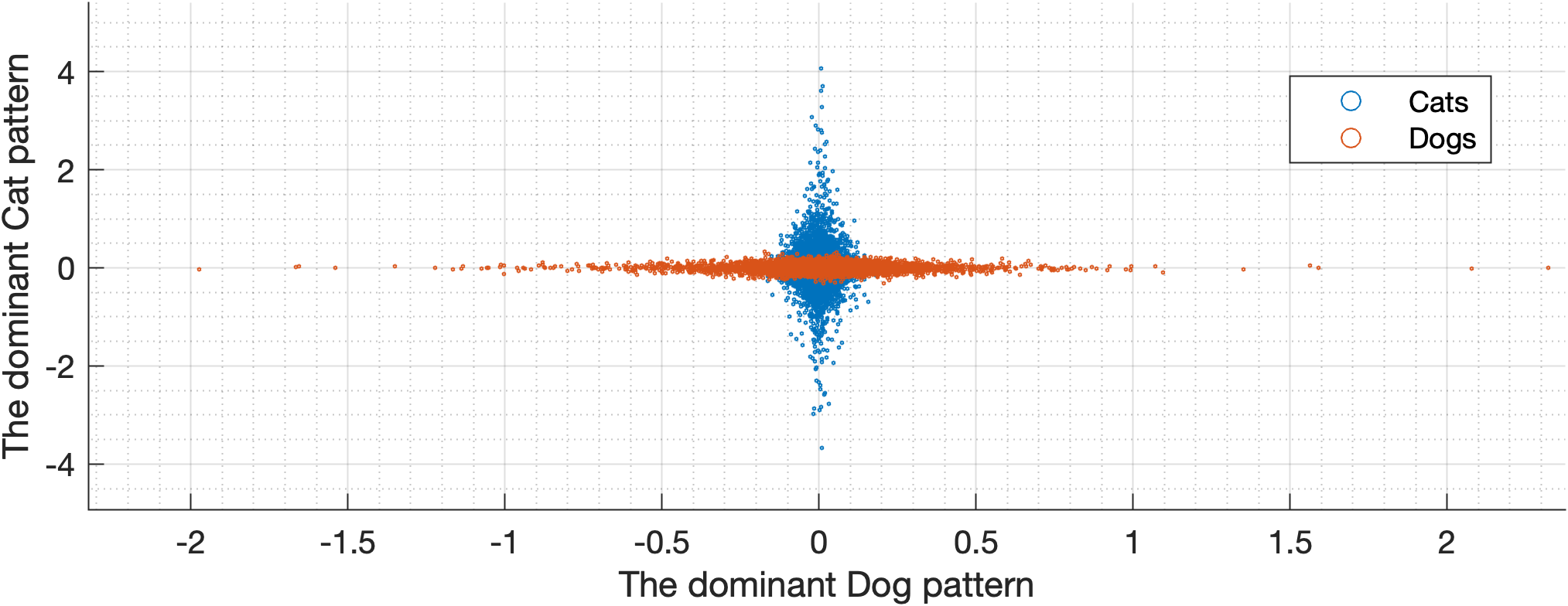
Figure 3: Contribution of most dominant dog pattern vs the most dominant cat pattern to all images in the dataset. There is a clear separation between classes, but there is also a considerable overlap near the origin (i.e., some images do not get considerable contributions from these two patterns.

Low rank approximation constructs image major structure, recognizable by deep neural nets. Each image is the summation of $m$ patterns, and each of those patterns has rank-1 in the wavelet space. Therefore, we can reconstruct low rank approximation of each image, using a relatively small number of those patterns. Figure 4 shows the evolution of one cat image as $j$ moves from 1 to $m$. For example, the image at the far left of this Figure, is the result of $\sum_{j=1}^{100}\sigma_{j}U_{i}(:,j)V_{i}(j,:)$ and the image at the far right is the result of $\sum_{j=1}^{3000}\sigma_{j}U_{i}(:,j)V_{i}(j,:)$.

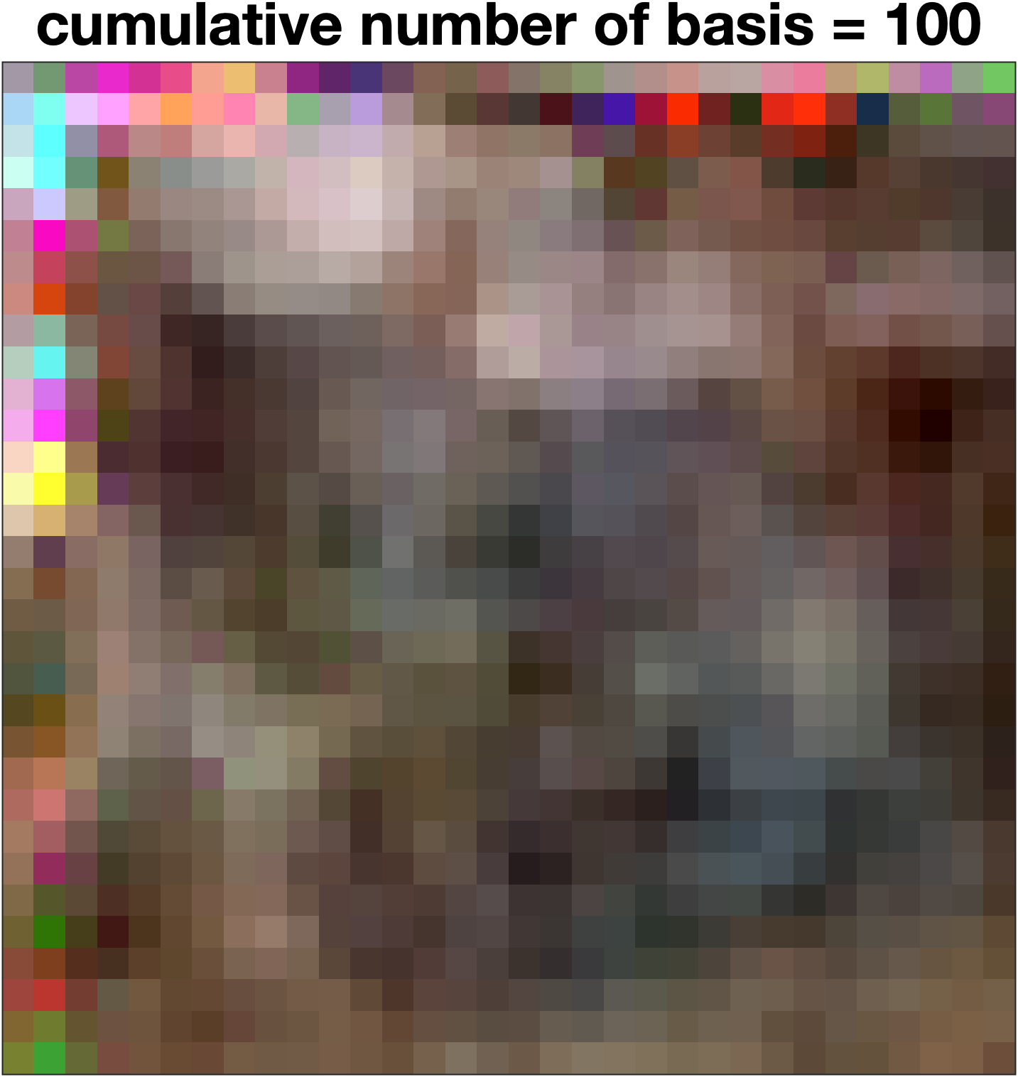
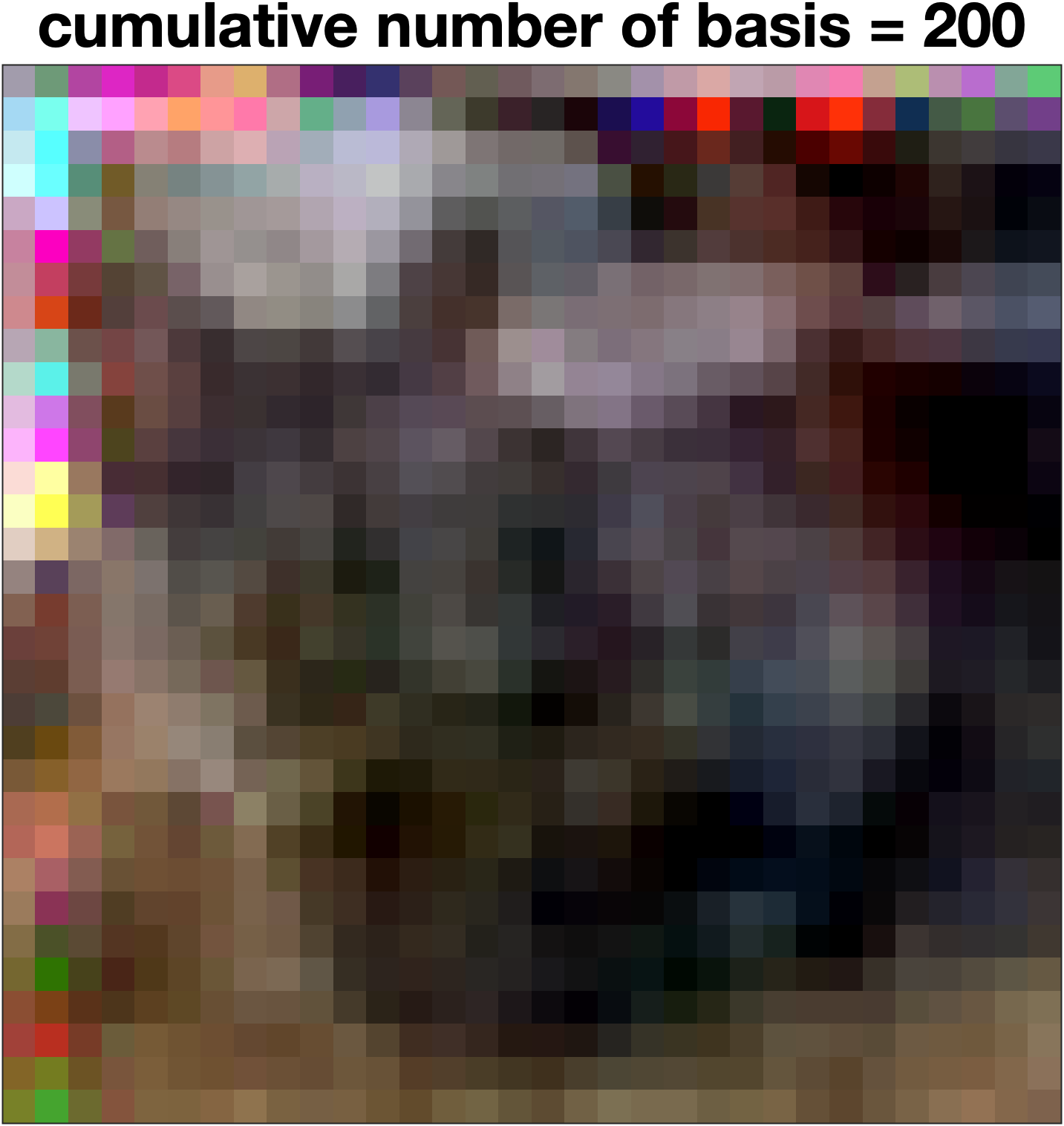
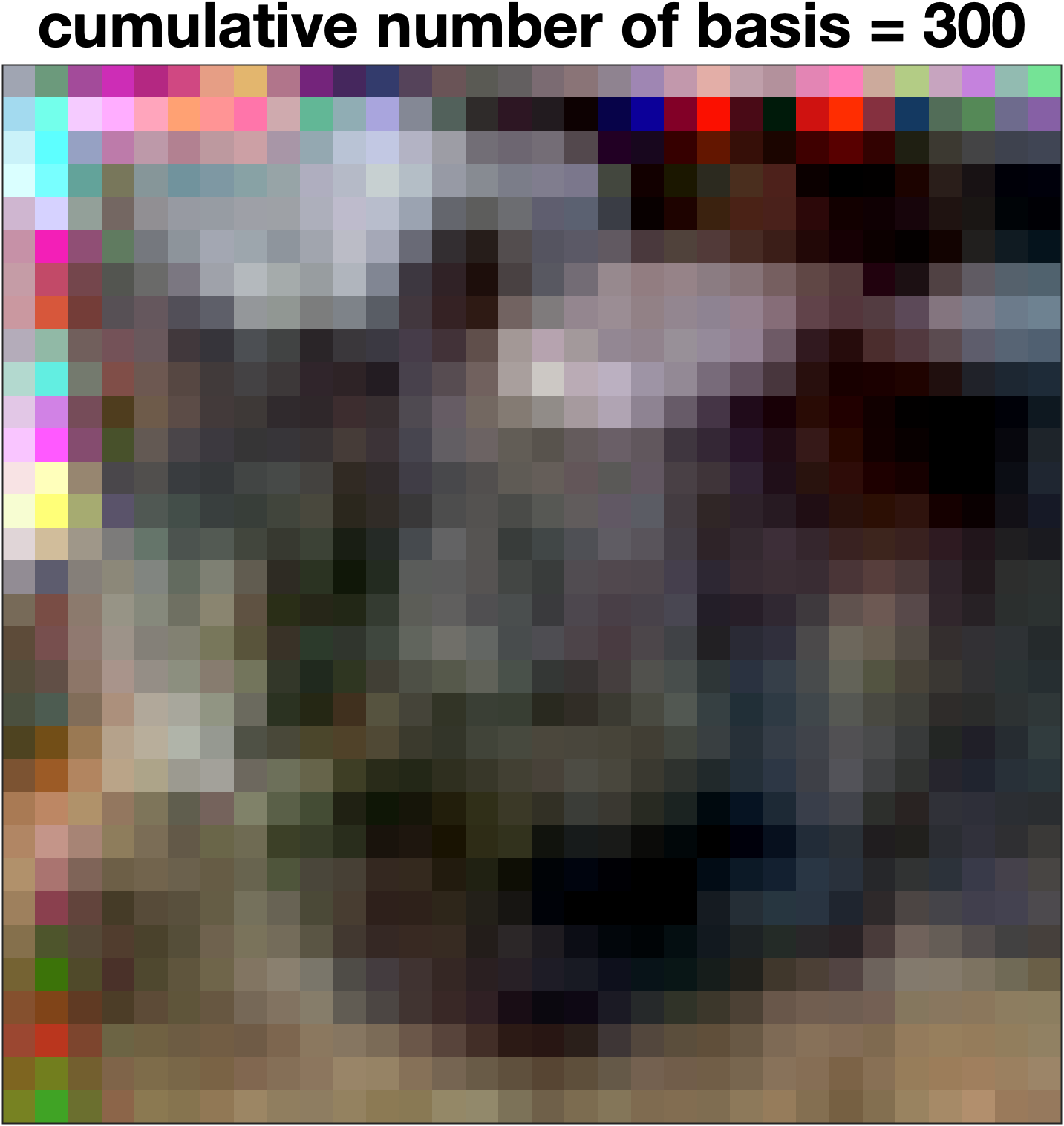
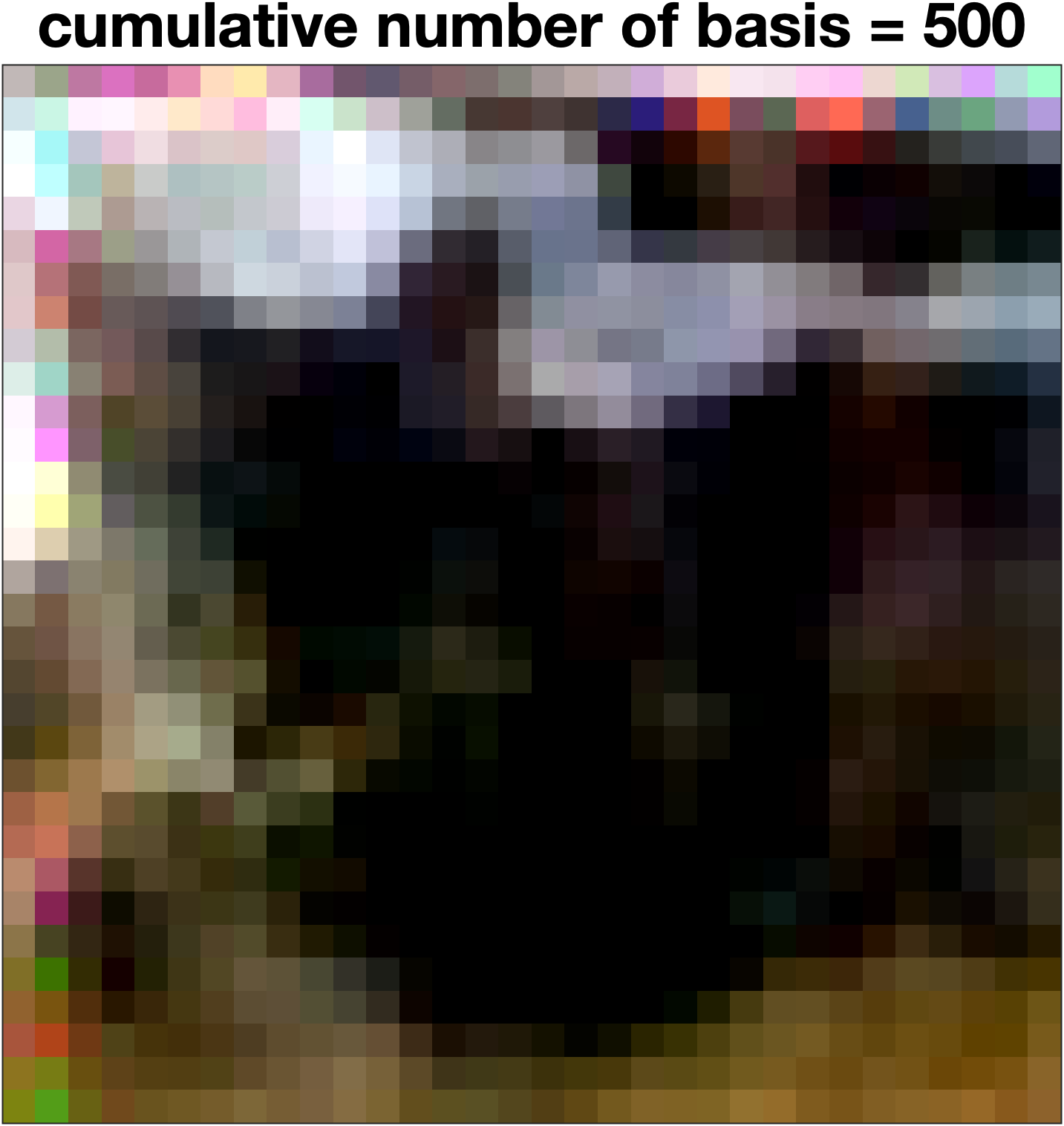
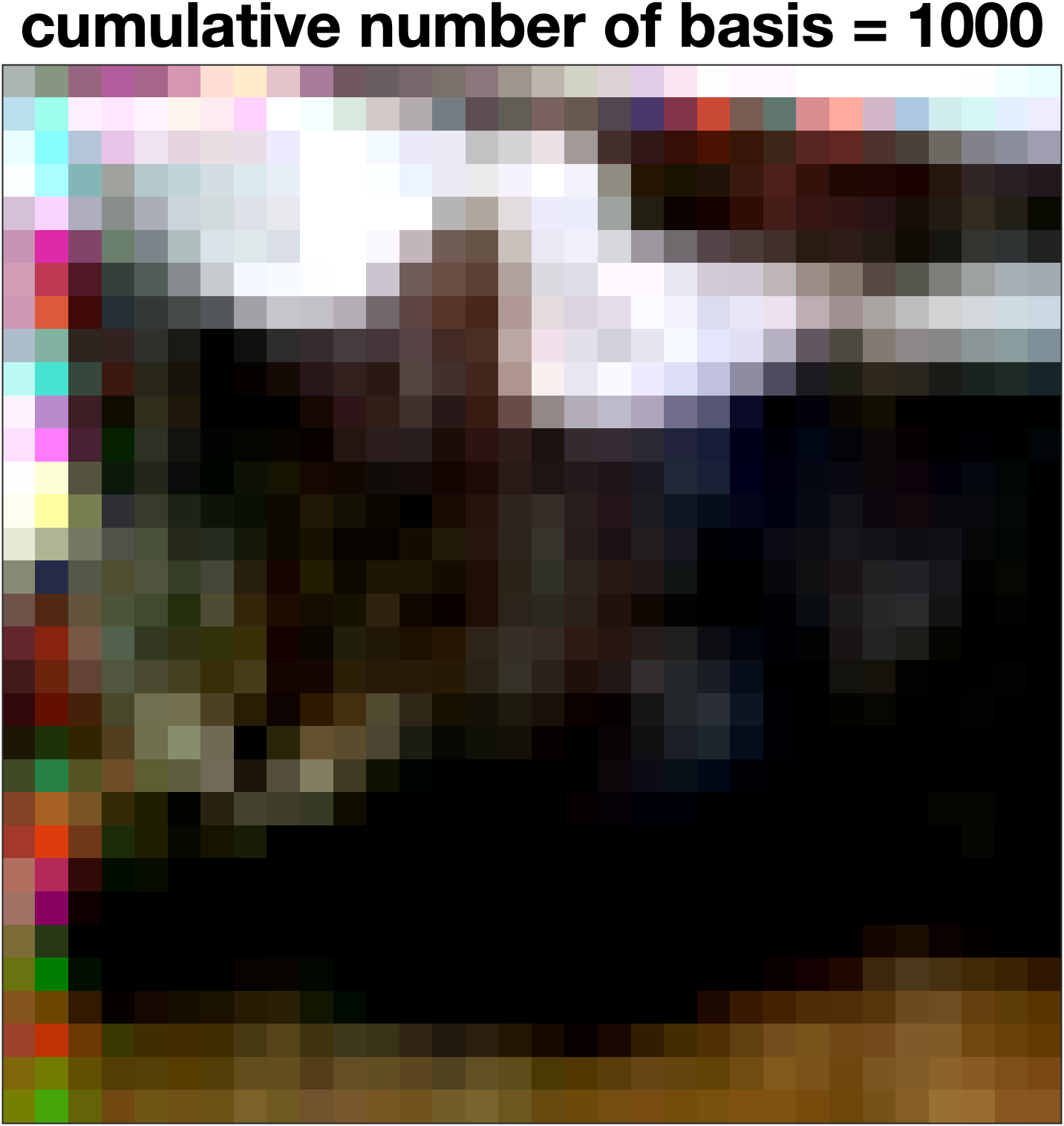
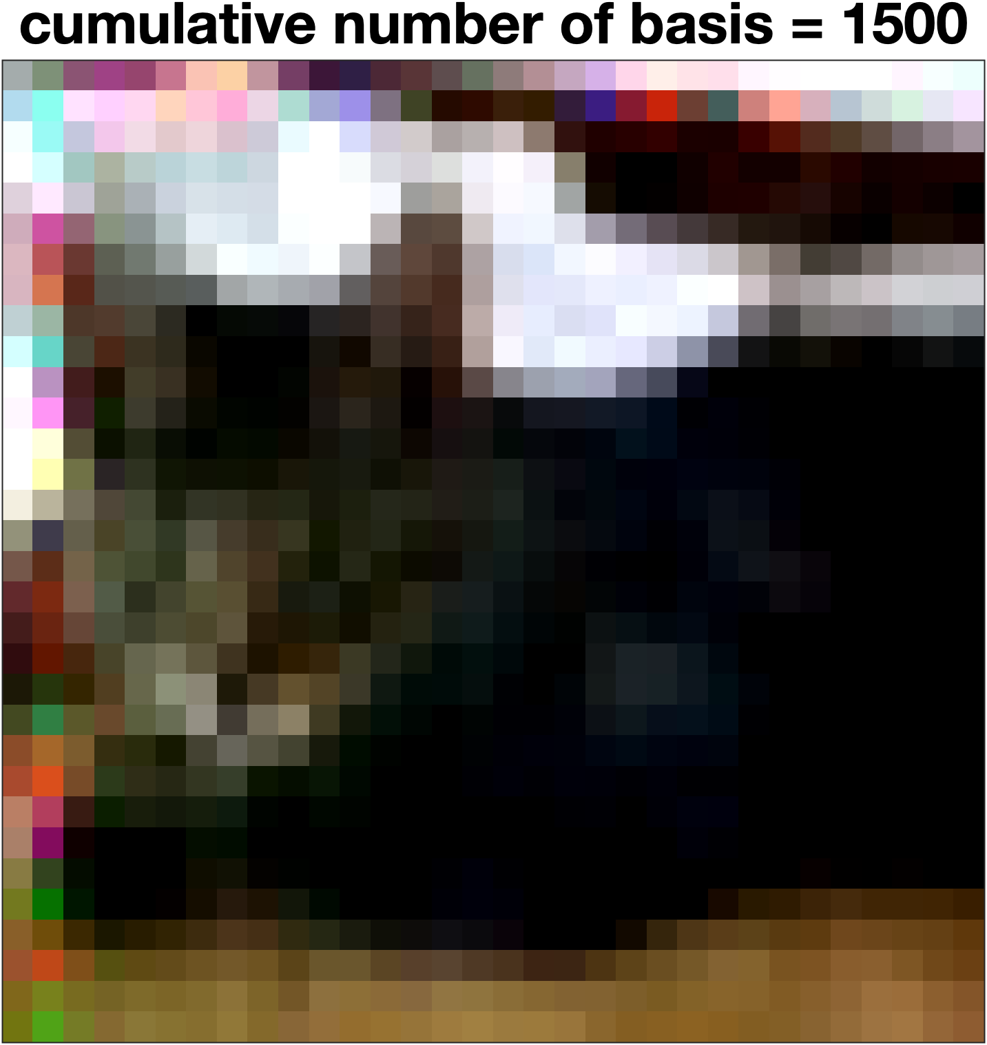
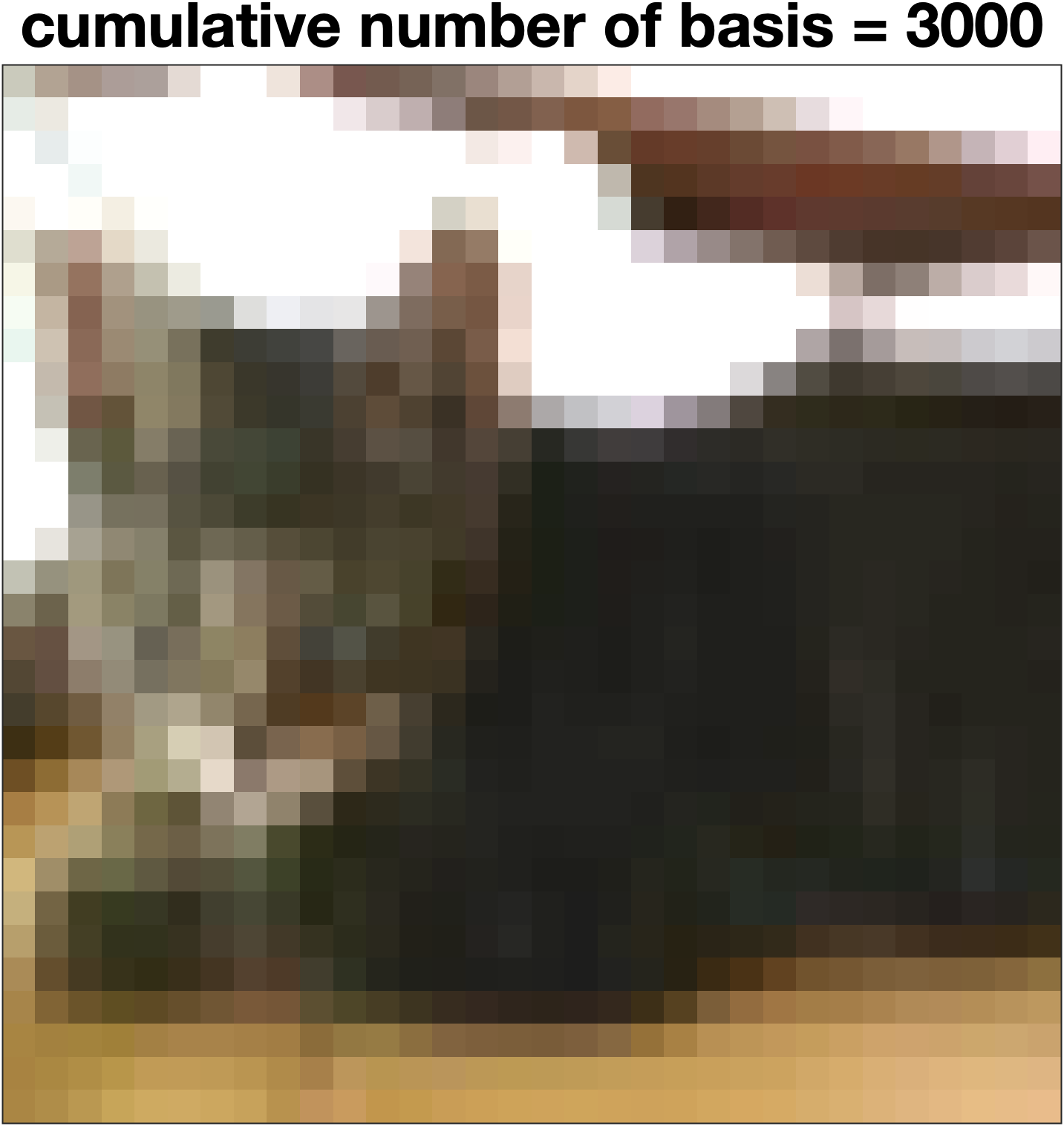
Figure 4: Images reconstructed by cumulatively adding rank-1 patterns in $V$. We see that for many images, the main structure and its distinctive features are obtained by adding a relatively small portion of patterns in the wavelet space. This is the first training image of Cat class.

Figure 5 shows the change in the residual, where the residual is the Frobenius norm between the original image and the reconstructed image from the wavelet space, during the process of adding rank-1 images. We present similar results for more images in Appendix B.

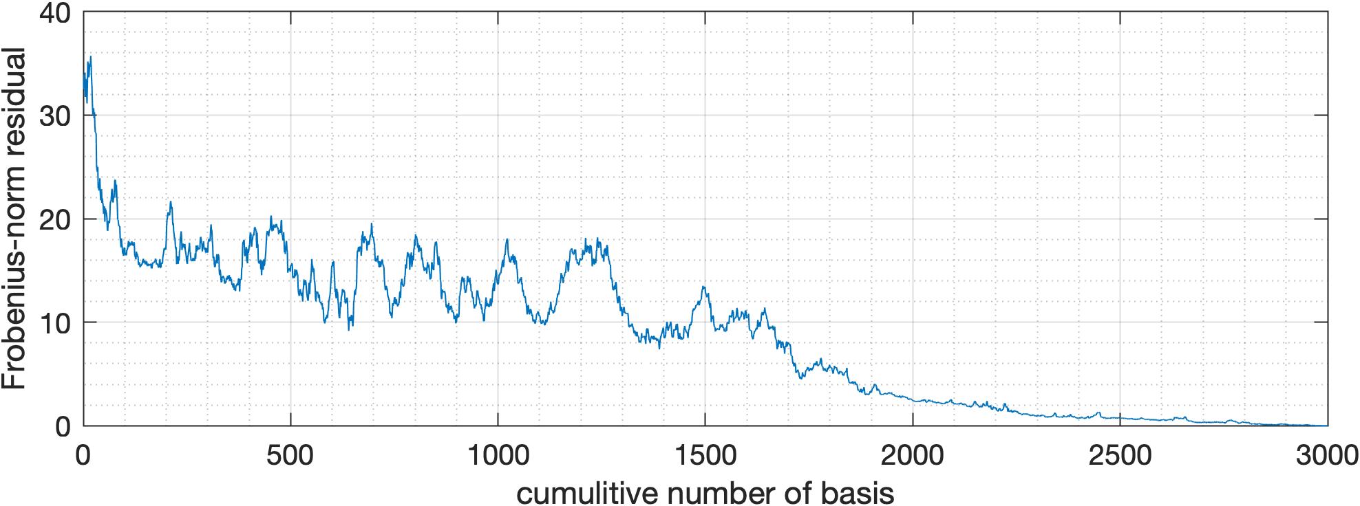
Figure 5: Residual of reconstructed image from the wavelet coefficients as we add more rank-1 patterns to it. The residual usually decreases during the process, implying that most rank-1 patterns are individually a useful contribution to the original image.

Complexity of images interpreted via the left basis. The left basis $U_{i}$ determines how the right basis vectors of $V$ should be put together in order to obtain the image. Each row of $U_{i}$ corresponds to one image in $D_{i}$. The rows of $U$ that have smaller norms correspond to images that are simpler, i.e., made of fewer components, e.g., Figure 6(a). The rows of $U$ with larger norm correspond to images with more components, e.g., Figure 6(b). Additionally, one can investigate the sparsity of rows of the left basis, which we leave in favor of brevity.

(a) Images with smaller norm in left basis

(b) Images with higher norm in left basis

Figure 6: Complexity of images reflected through the left basis. (a) Images with smaller norm in left basis look simpler and have fewer distinctive features; (b) images with higher norm in left basis do not look simple and have several distinctive features.

Distinctive Patterns Discovered for All classes of CIFAR-10. As we saw previously, one of the important aspects of our interpretation is to associate the patterns to specific classes, which is done by comparing the singular values. When we repeat this analysis for all 10 classes of this dataset, we see that patterns emerge that are associated with more than 1 class.

Figure 7 shows the log of 1,000 singular values obtained for this dataset. Clearly, classes of Truck and Automobile have the highest singular values for many of the patterns, which makes them distinguishable from the others, but not so helpful to distinguish each class from all other classes. This suggests that our approach could be useful in a hierarchical setting where classes are grouped and then analyzed further. Alternatively, one could consider using our method for pairwise comparison of classes as in Siamese networks (Bertinetto et al., 2016). We next make the labels random to see how it affects the learnability of dataset.

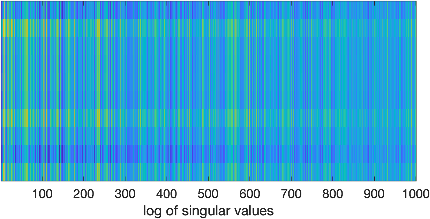
(a) Correct labels

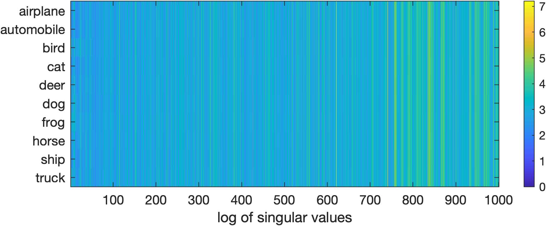
(b) Random labels

Figure 7: The first 1,000 singular values of $\Sigma_{i}$’s for all 10 classes of CIFAR-10 dataset. Note that we have used logarithmic transformation in this figure. Any association between patterns and classes fades away, when we make the labels random.

Labeling the images randomly to diminish learn-ability. We repeat the spectral analysis to see if patterns will be associated with classes or not, when labels are random. We know that deep learning models can achieve perfect accuracy on this training set, even when all the images are labeled randomly, and one would not be able to detect the randomness of labels just by training a model. We show that our method reveals whether there is learnable classification information present in the training set, useful in practice, and also useful for studying the concept of memorization vs learning. When we make the labels random for all images, the decomposition we obtain is very different and ambiguous. Specifically, the singular values become uniform across classes, as shown in Figure 7(b).

To demonstrate this effect more clearly, we measure the angular distance between the singular values of two classes of Ship and Truck, with the correct labels (Figure 7(a)) and with random labels (Figure 7(b)). As shown in Figure 8, in the correct label case, singular values are discriminitive between the two classes, i.e., for many patterns, the angular distance is noticeable (blue line). However, in the random label case, the angular distance between singular values are close to zero for almost all the patterns (red line).

If we limit the portion of randomly labeled data, for example, to 20% and keep the correct labels for the rest of images, we see that the obtained results are not very different from the results we obtained for the correctly labeled data. Repeating this with different portions of random labels shows that the disassociation between patterns and labels is directly related to the portion of random labels.

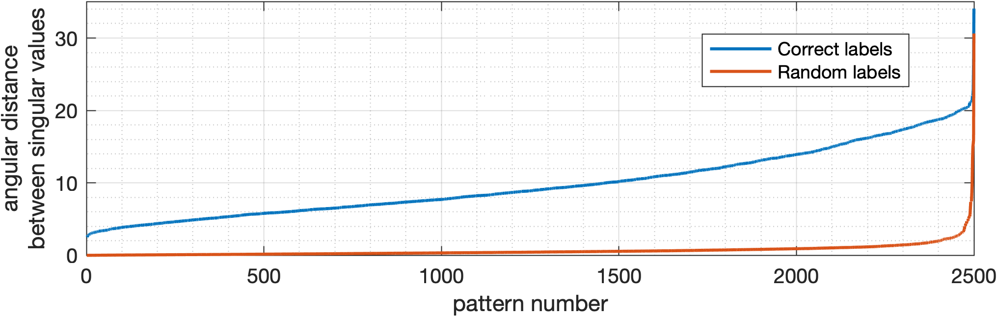
Figure 8: Angular distance (absolute value) between singular values of classes Ship and Truck, when labels are correct (blue) and when labels are random (red). Randomizing the labels leads to collapse of angular distances and makes the patterns disassociated from the classes.

6 Conclusions and future work

Here, we showed that spectral decomposition of image classification datasets in the wavelet space can extract the patterns that distinguish each class from the others. We decomposed each image as the summation of finite number of rank-1 images in the wavelet space and showed that low rank approximation to images can capture the classification information to classify them. Our method can also be used to verify existence of learnable classification information in datasets, useful for studies on memorization vs learning of deep models, and also useful in practice for analyzing unfamiliar datasets.

Future directions of research can be to study the adversarial robustness, generalization, and functional behavior of deep classifiers with respect to rank-1 patterns extracted from datasets, and also to study the patterns in relation to deep features.

Appendix A The choice of wavelet basis and the data extracted

A.1 CIFAR-10 dataset in the wavelet space

About the choice for wavelet basis, it seems natural to choose a 2D basis for the images typically used for classification. A 1D wavelet basis will not be as capable to extract all the information we need from images. A 3D wavelets did not show an advantage over 2D wavelets in our numerical experiments, but it might be advantageous in certain datasets.

For the CIFAR-10 dataset, we experimented with Haar and also the first 5 Daubechies wavelets in 2D. We observed that the data extracted with Daubechies-2 was slightly more informative (higher rank), compared to Haar and Daubechies-1. But, we did not find the information extracted with Daubechies-3 to 5 to be more informative. So, our experiments on this dataset are with Daubechies-2 wavelets. This wavelet basis extracts 3,468 features from each image in this dataset, but not all of these features are influential in our pattern analysis for classification. Hence, we chose 3,000 of those coefficients using RR-QR algorithm.

We note that the end result of our analysis, e.g., the patterns extracted in the tensor decomposition were not noticeably sensitive to the choice of wavelet basis.

Figure A1 shows only the first 1,500 columns for each $\mathcal{D}_{i}$, to show how the data generally looks like. But, note that we actually used 3,000 wavelet coefficients in our experiments.

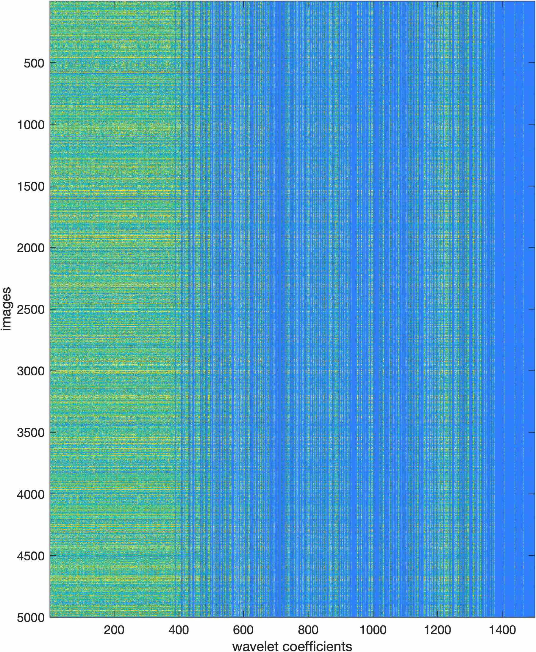
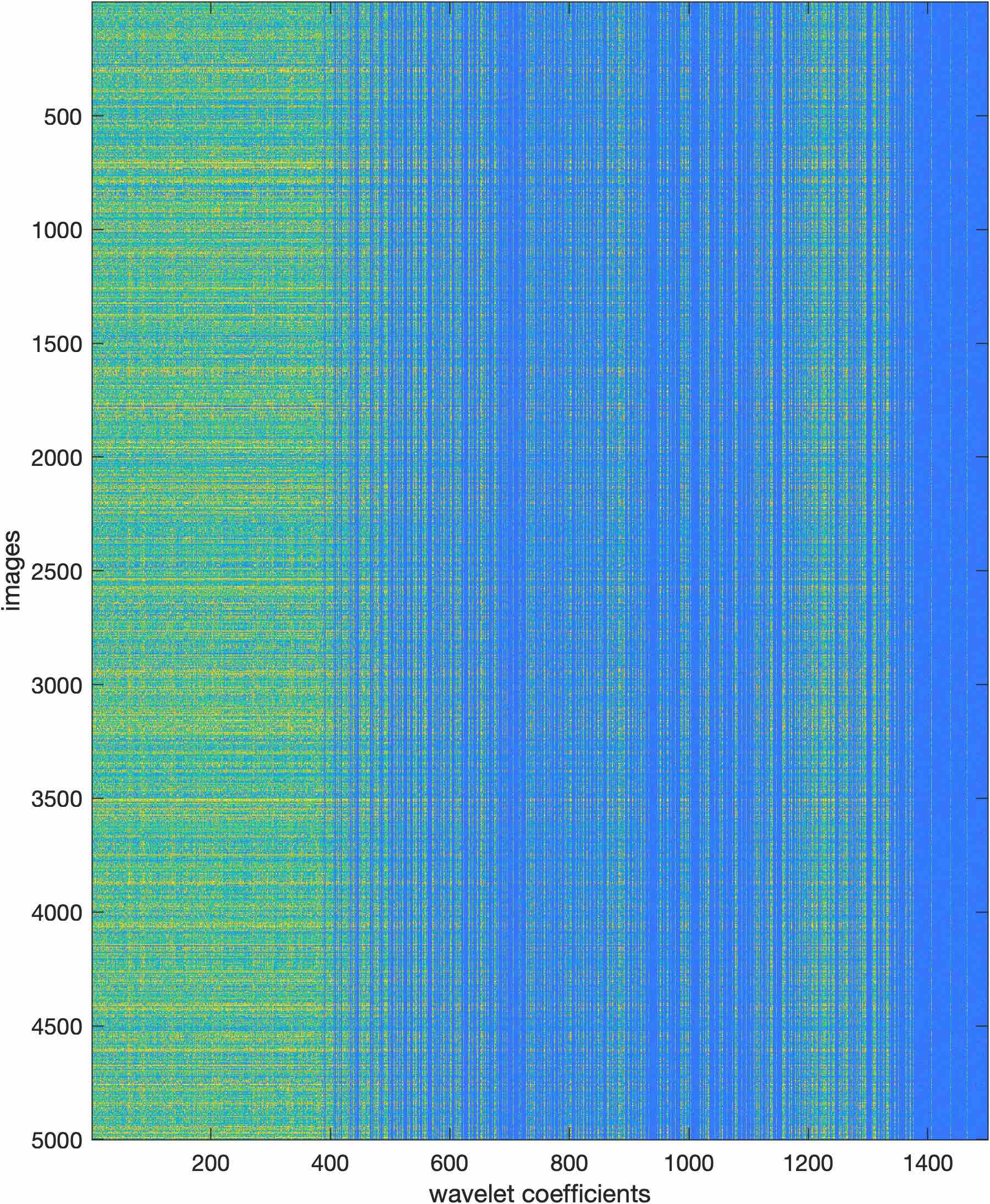
Figure A1: Matrix of wavelet coefficients for training images for classes of Cats (left) and Dogs (right) in CIFAR-10 dataset. This figure shows the first 1,500 most influential wavelet coefficients of images, chosen by the RR-QR algorithm.

A.2 MNIST dataset in the wavelet space

For MNIST, again we did not find the choice of wavelet basis to be noticeable in the patterns extracted. We found the Daubechies-1 to transform the images similar to higher order Daubechies wavelets. We note that the data extracted from this dataset has significant redundancies and linear dependencies compared to the data extracted from CIFAR-10. This is to be expected because the images of MNIST are very simple compared to images of CIFAR-10.

Figure A2 shows each of the $\mathcal{D}_{i}$’s for the 10 classes of MNIST.

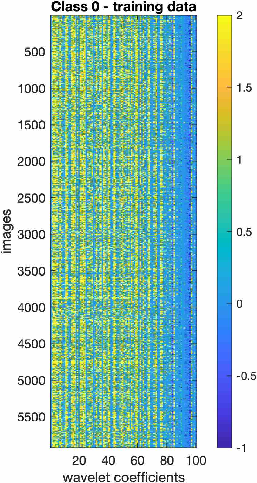
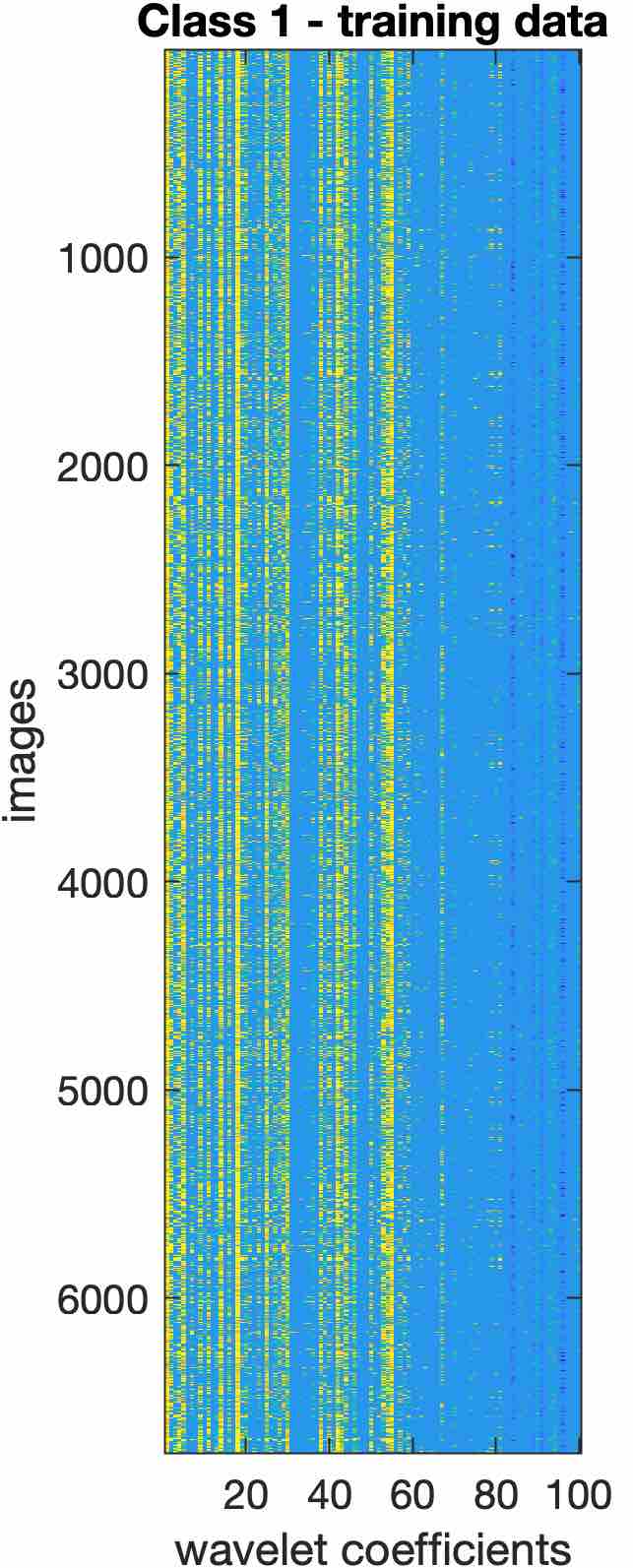
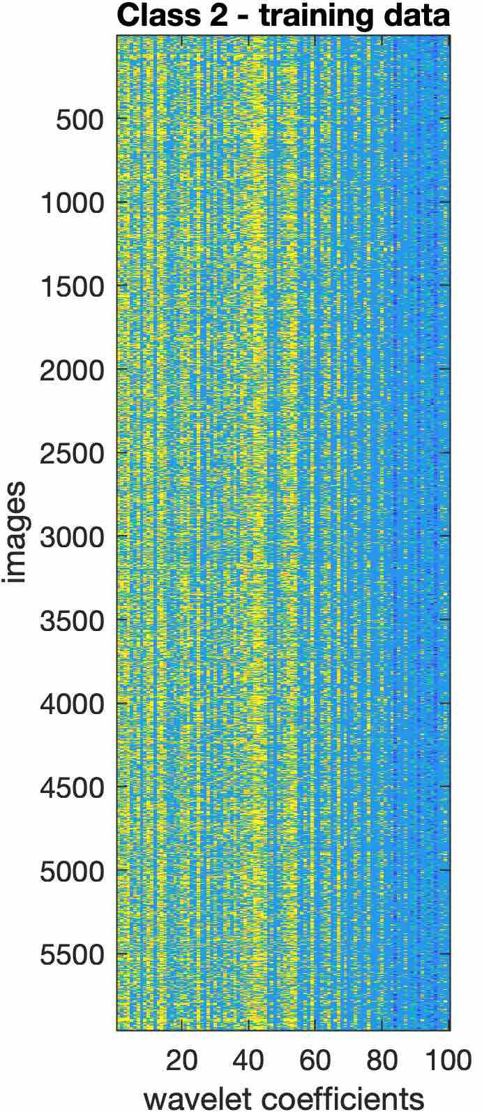
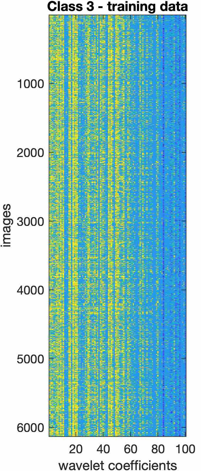
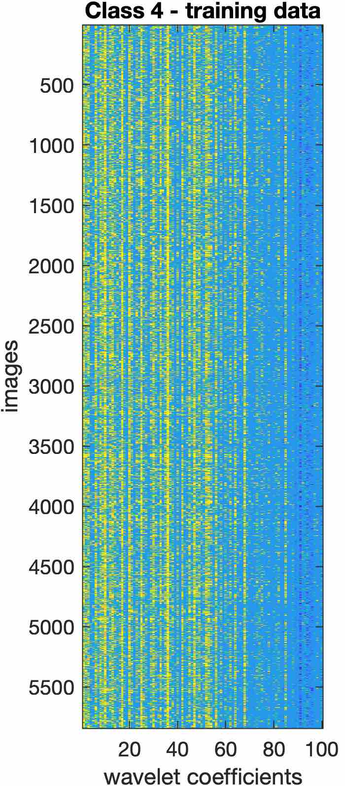
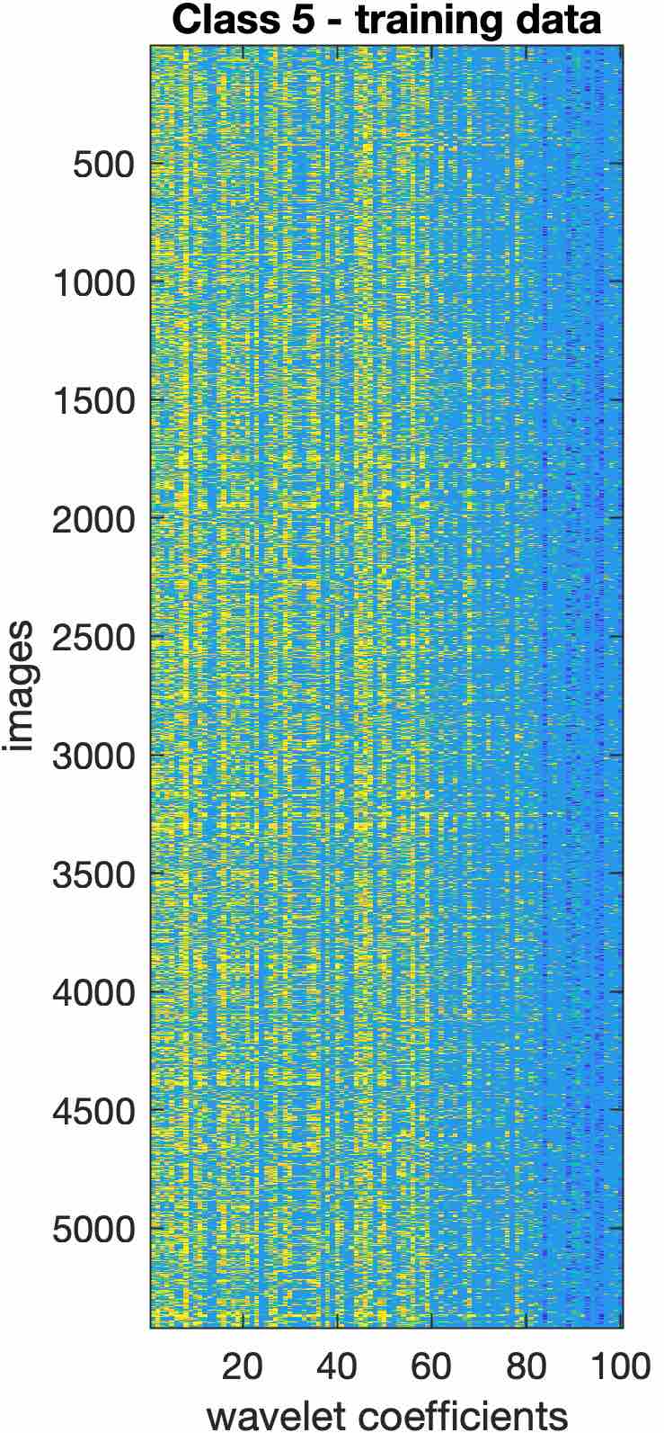
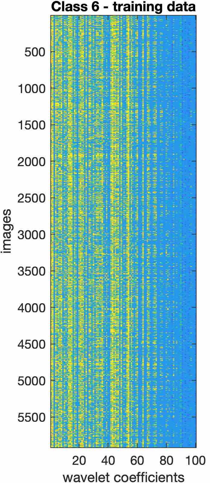
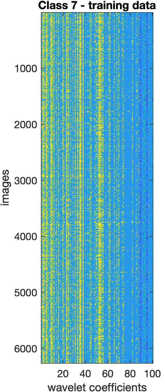
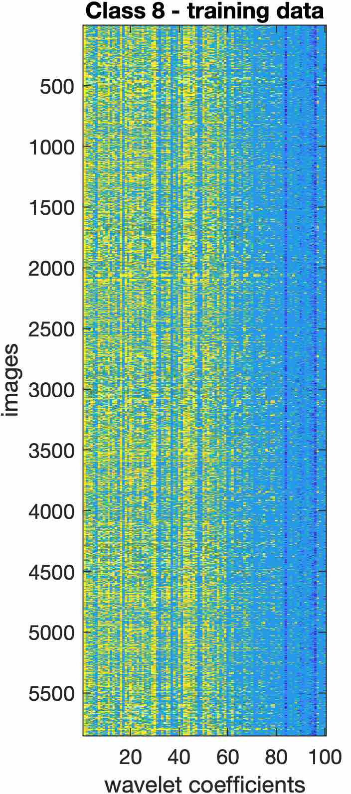
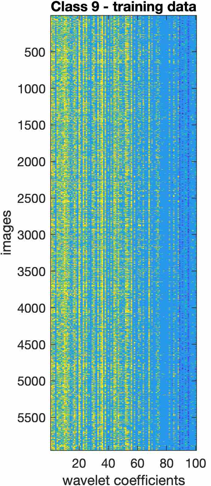
Figure A2: Matrix of wavelet coefficients for training images of 10 classes of MNIST dataset. Columns represent 100 of the most influential wavelet coefficients of images, chosen by the RR-QR algorithm. The same color scale is used for all figures.

Figure A3 shows the right basis $V$ which is common among all classes.

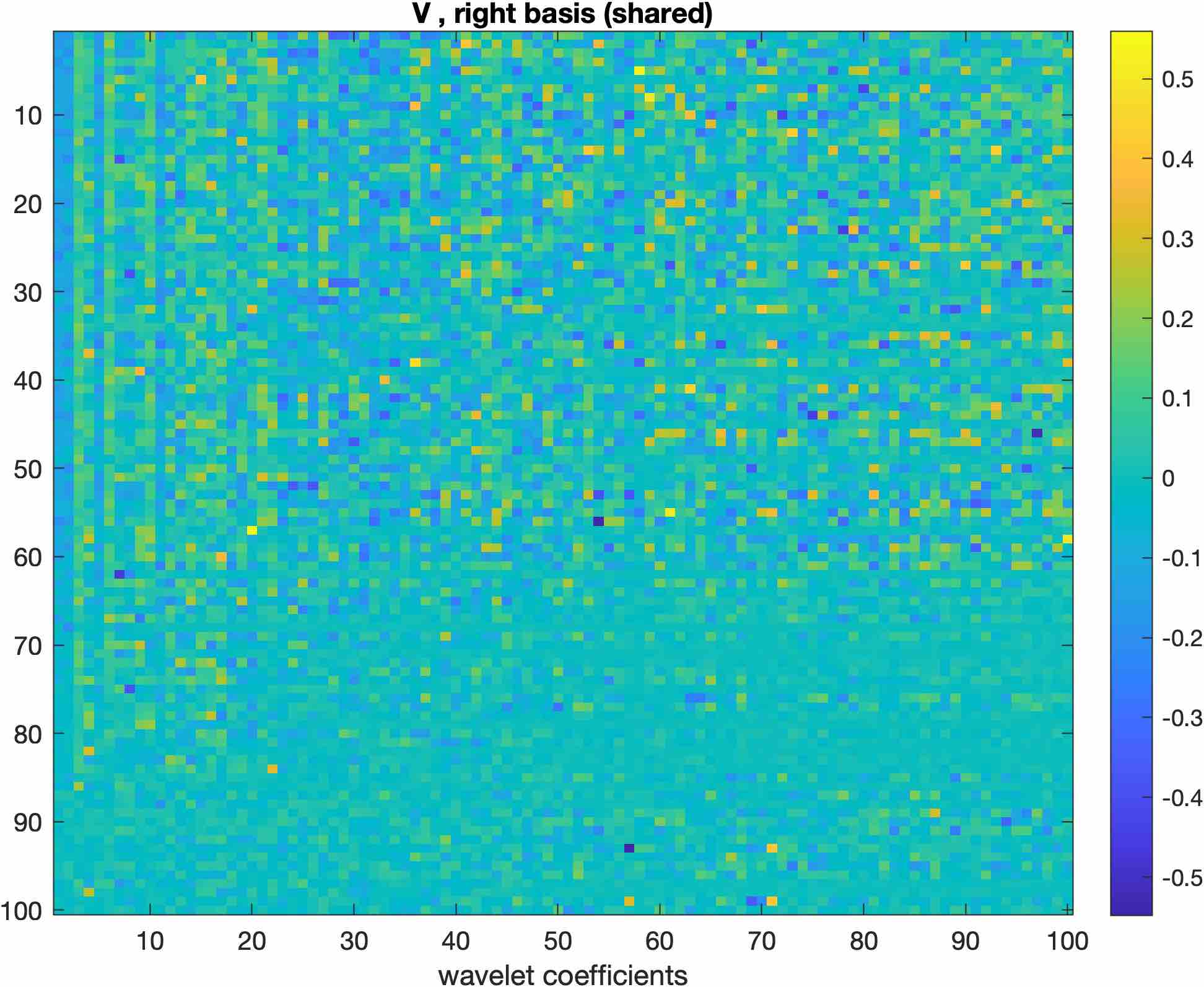
Figure A3: The right basis $V$ obtained from Higher Order GSVD, which is common among all classes of MNIST. Images in Figure D1 are reconstruction of specific columns of this matrix, back into the pixel space.

Appendix B Additional examples for reconstructing images as summation of rank-1 images

Here, we provide an example of writing a testing image as summation of rank-1 images obtained from the training set (in the wavelet space). Hence the same common basis obtained from all classes of training set, works for efficient decomposition of testing images, as well.

Figure B1 shows the reconstruction of the 3rd testing image of the Cat class in CIFAR-10.

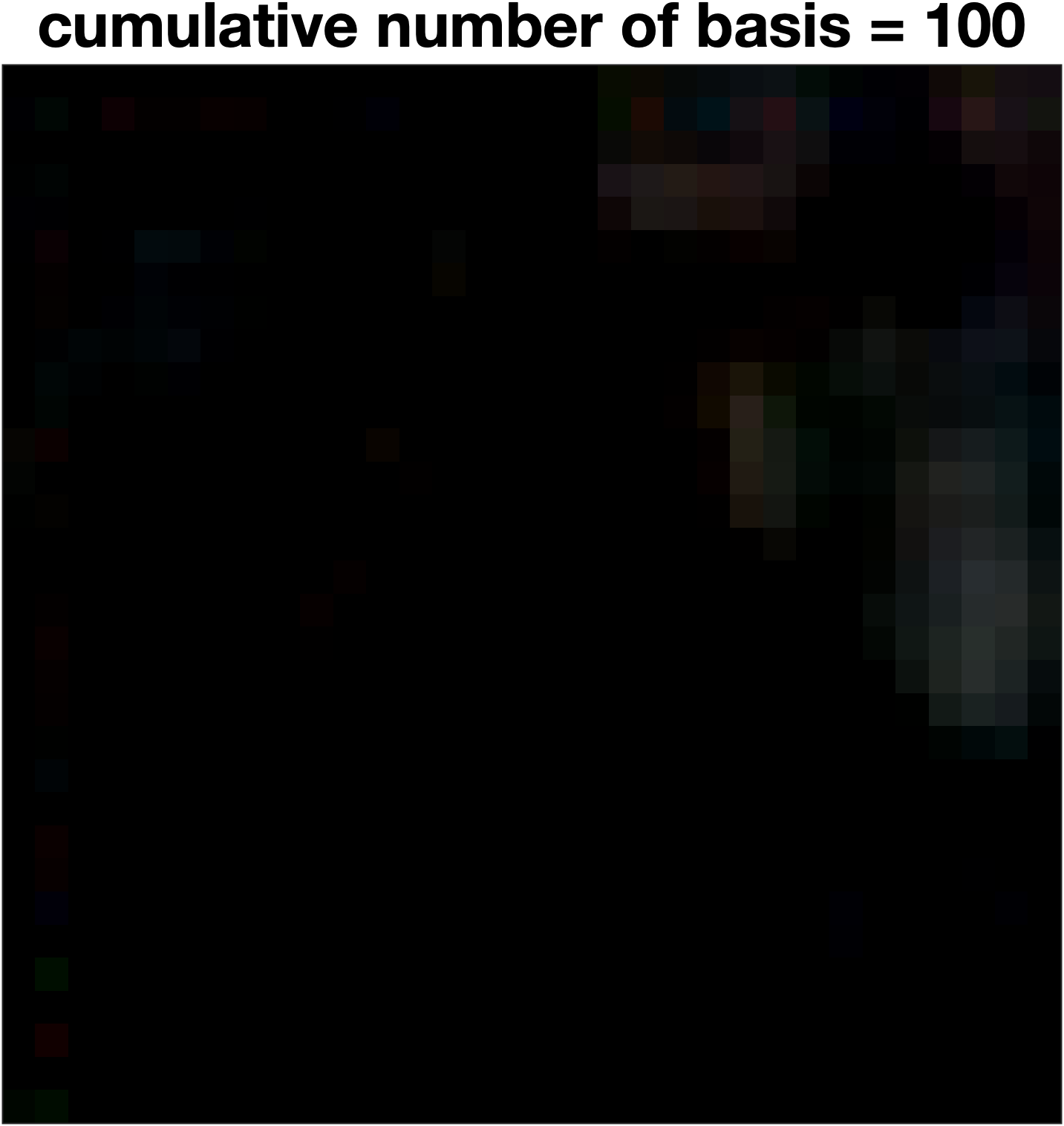
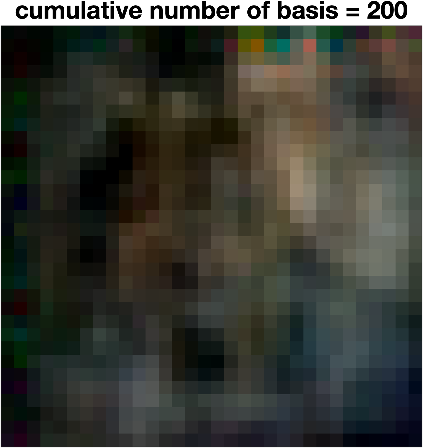
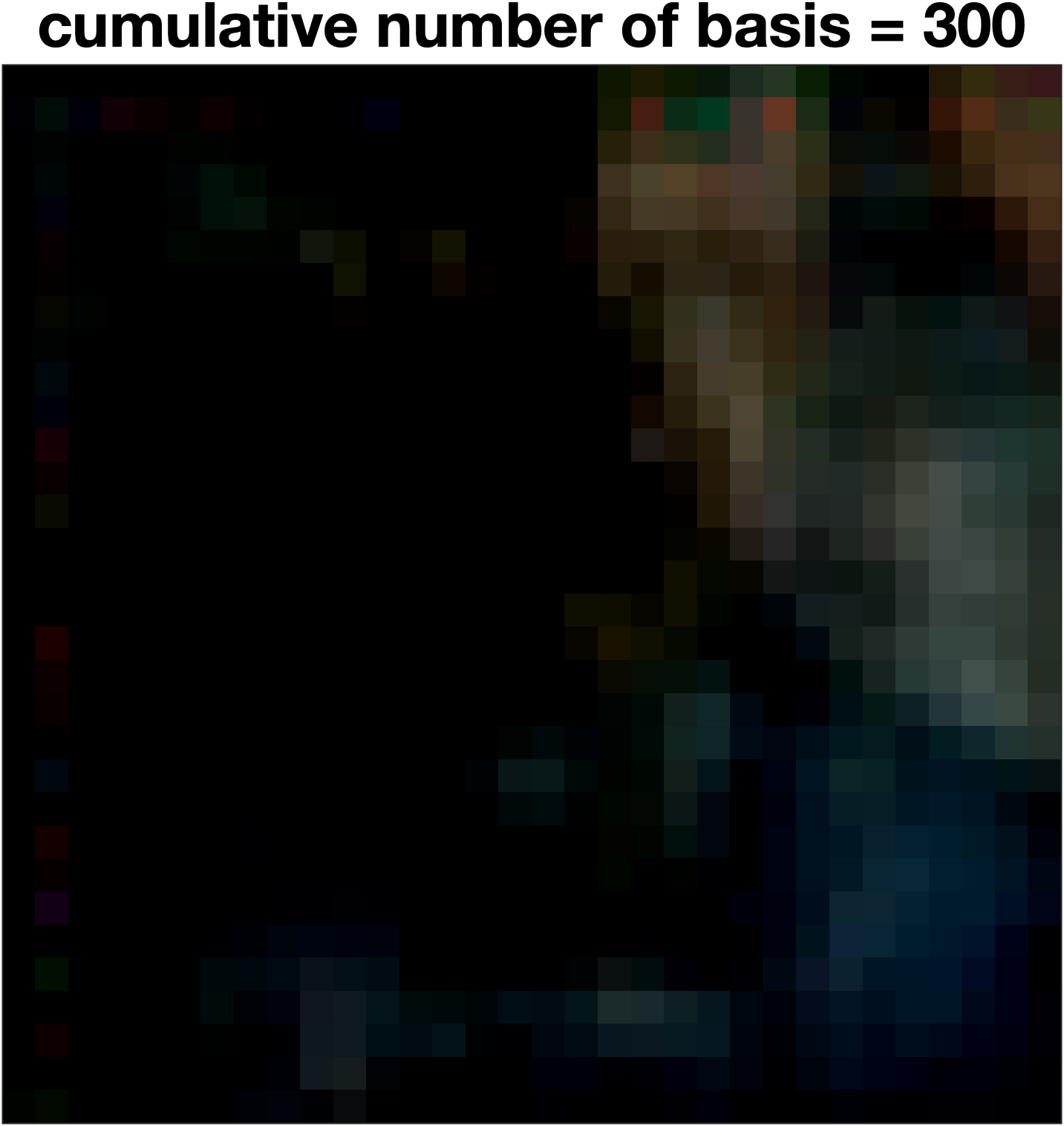
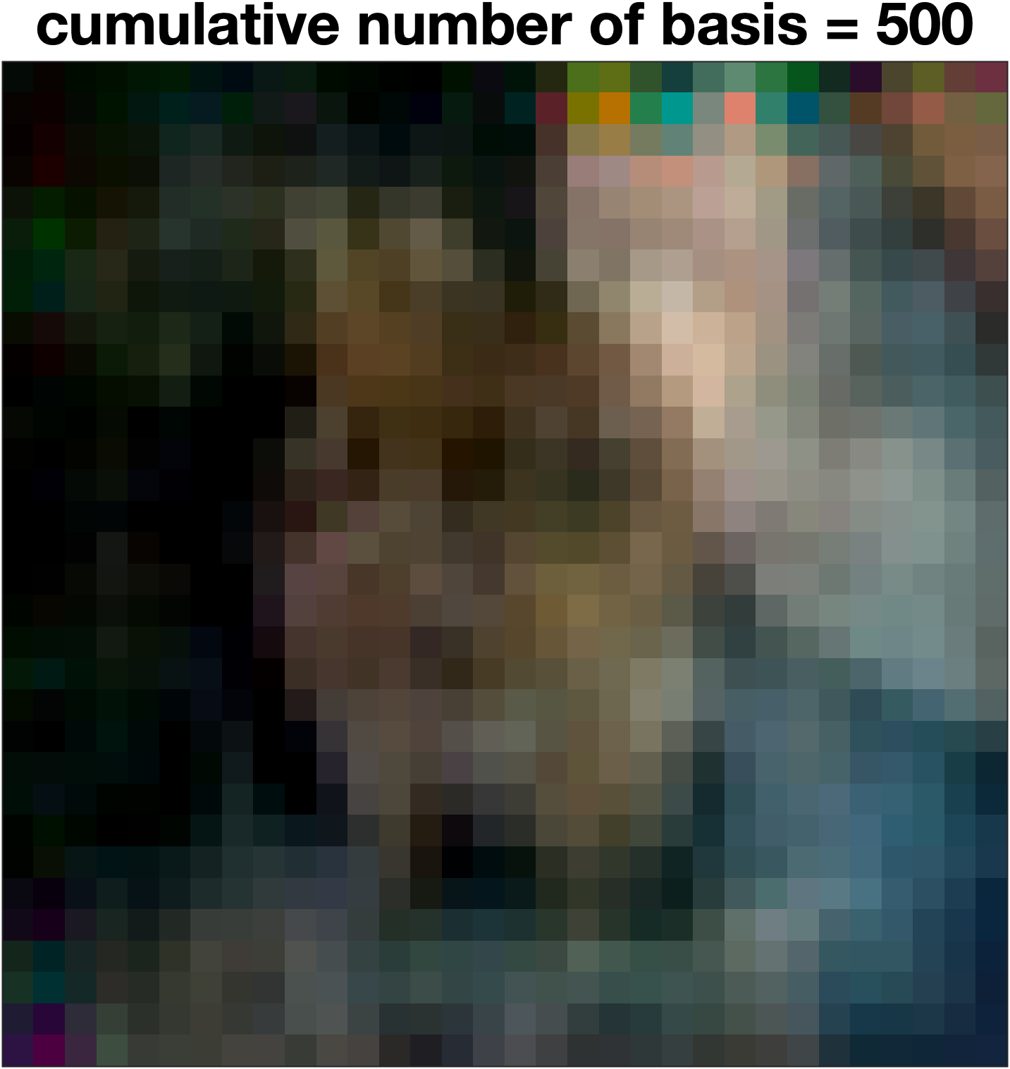
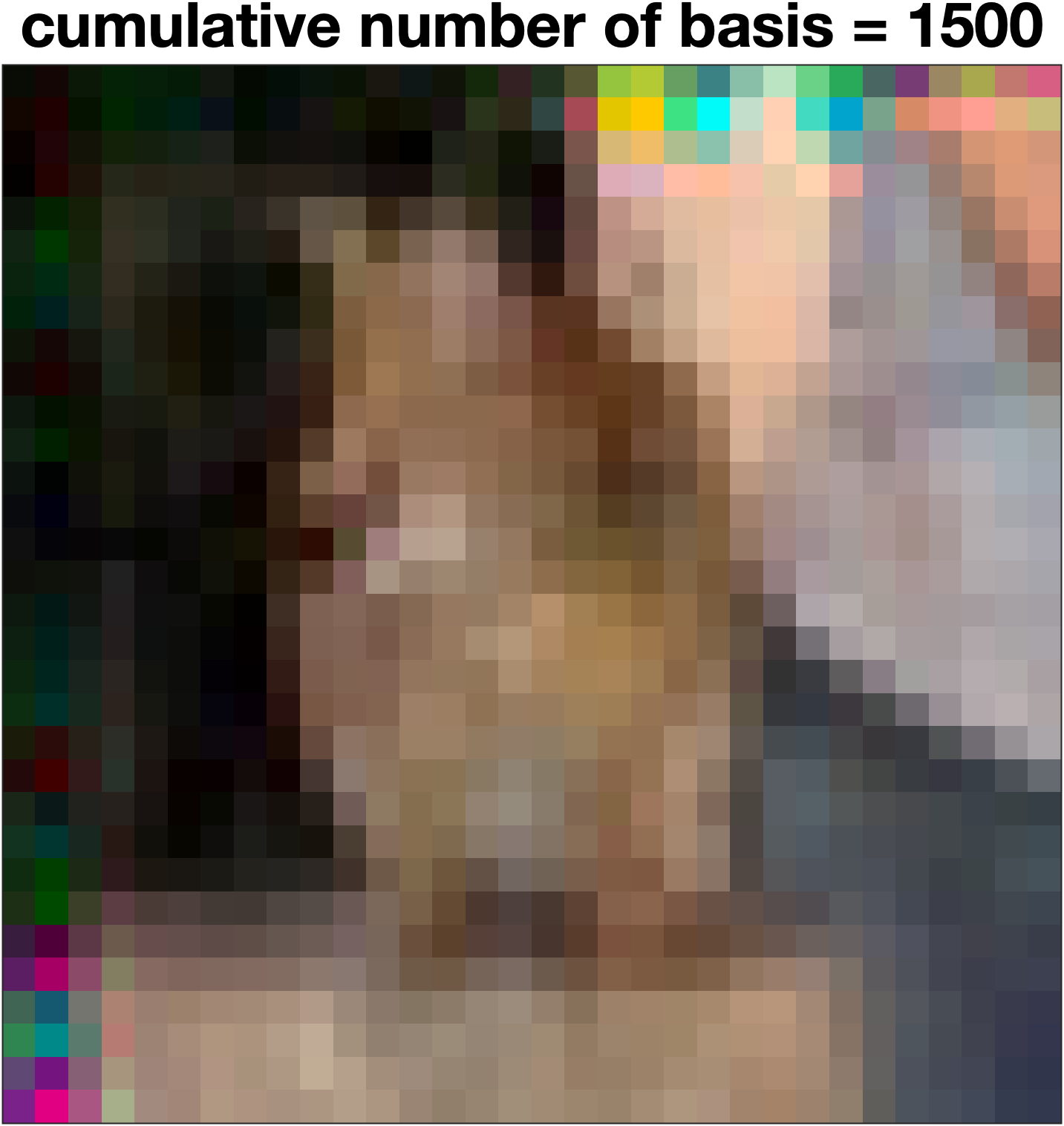
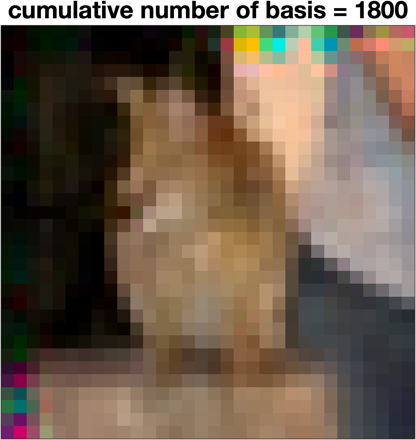
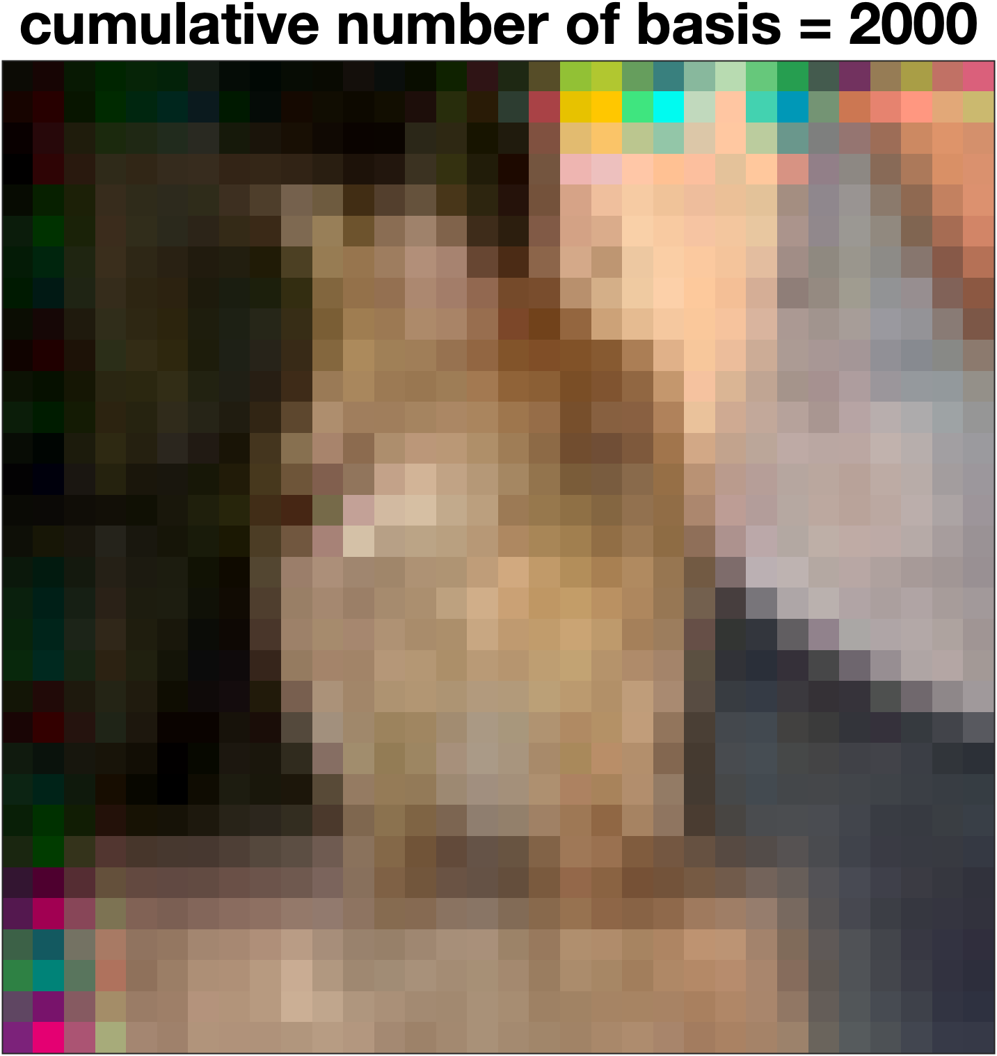
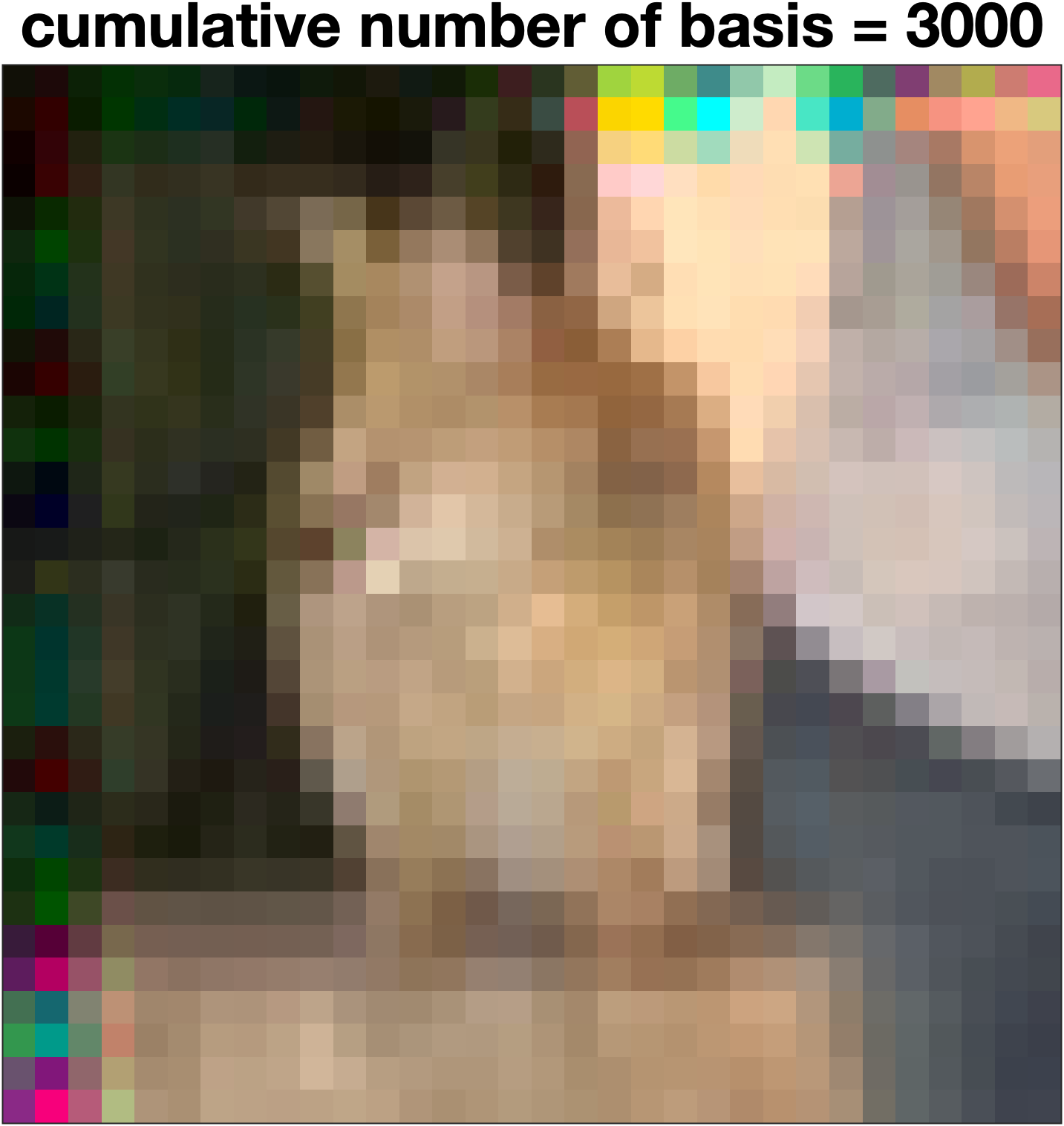
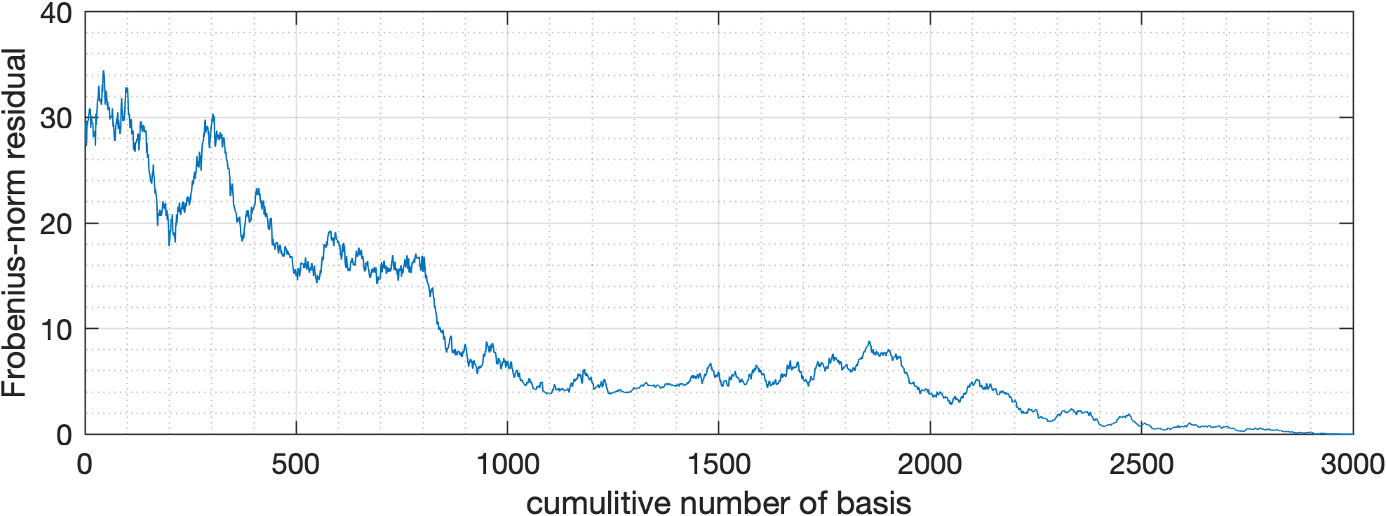
Figure B1: 3rd testing image of the Cat class in CIFAR-10. We have used the common right basis obtained from training set to decompose this image into rank-1 images.

Figure B2 shows the reconstruction of a testing image of Cat class that is misclassified by state of art model on CIFAR-10.

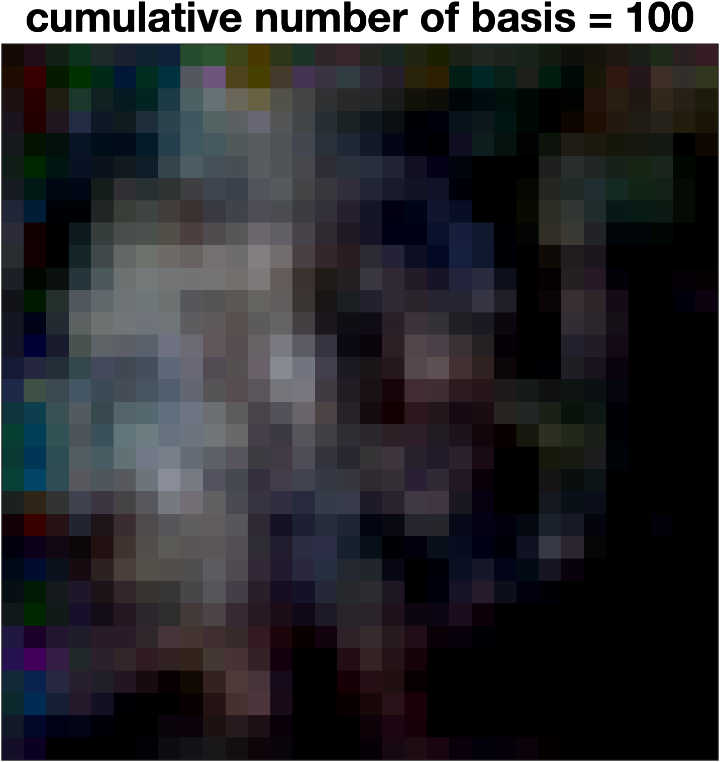
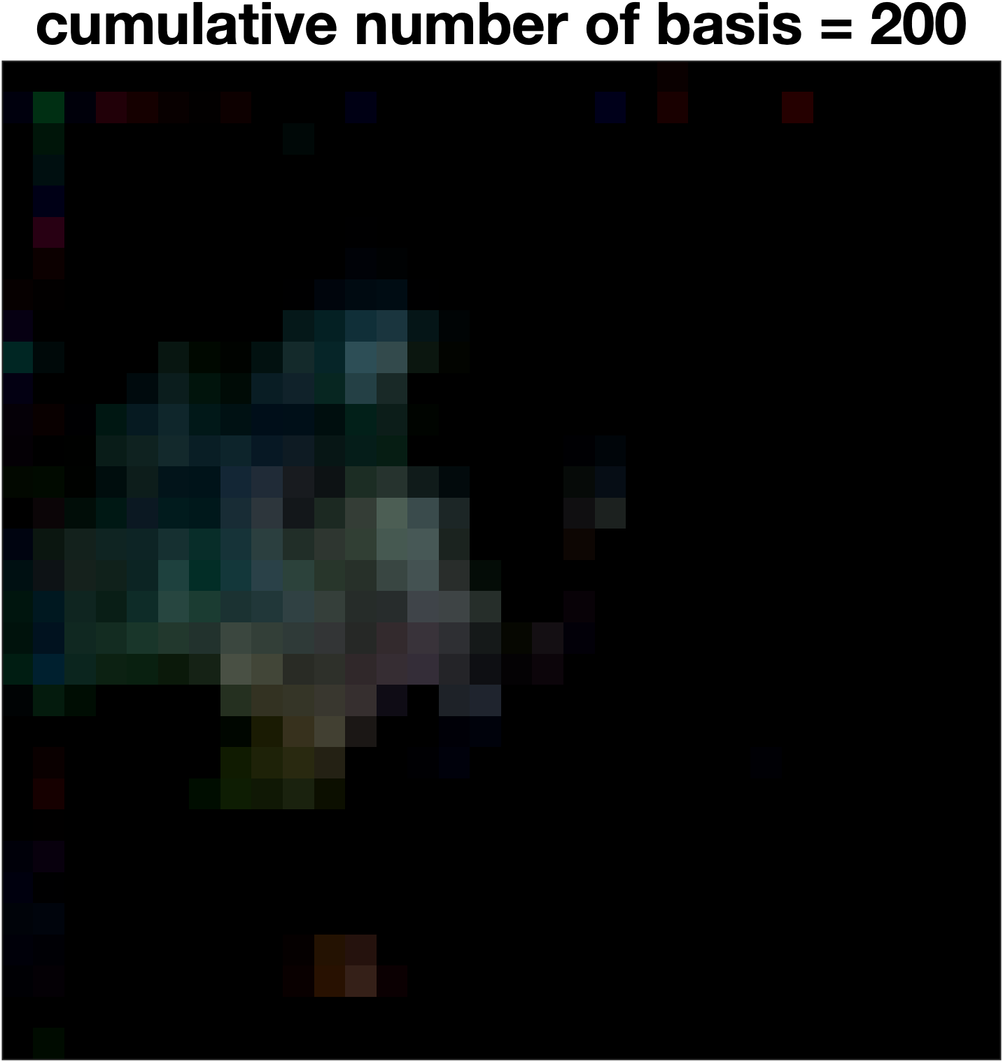
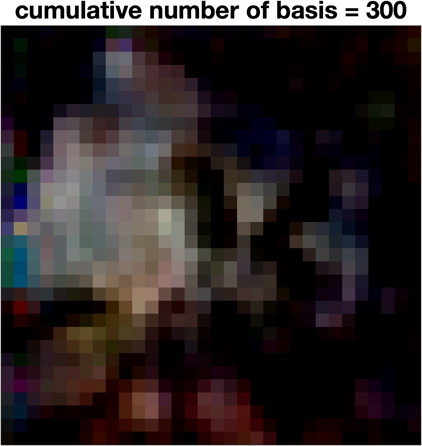
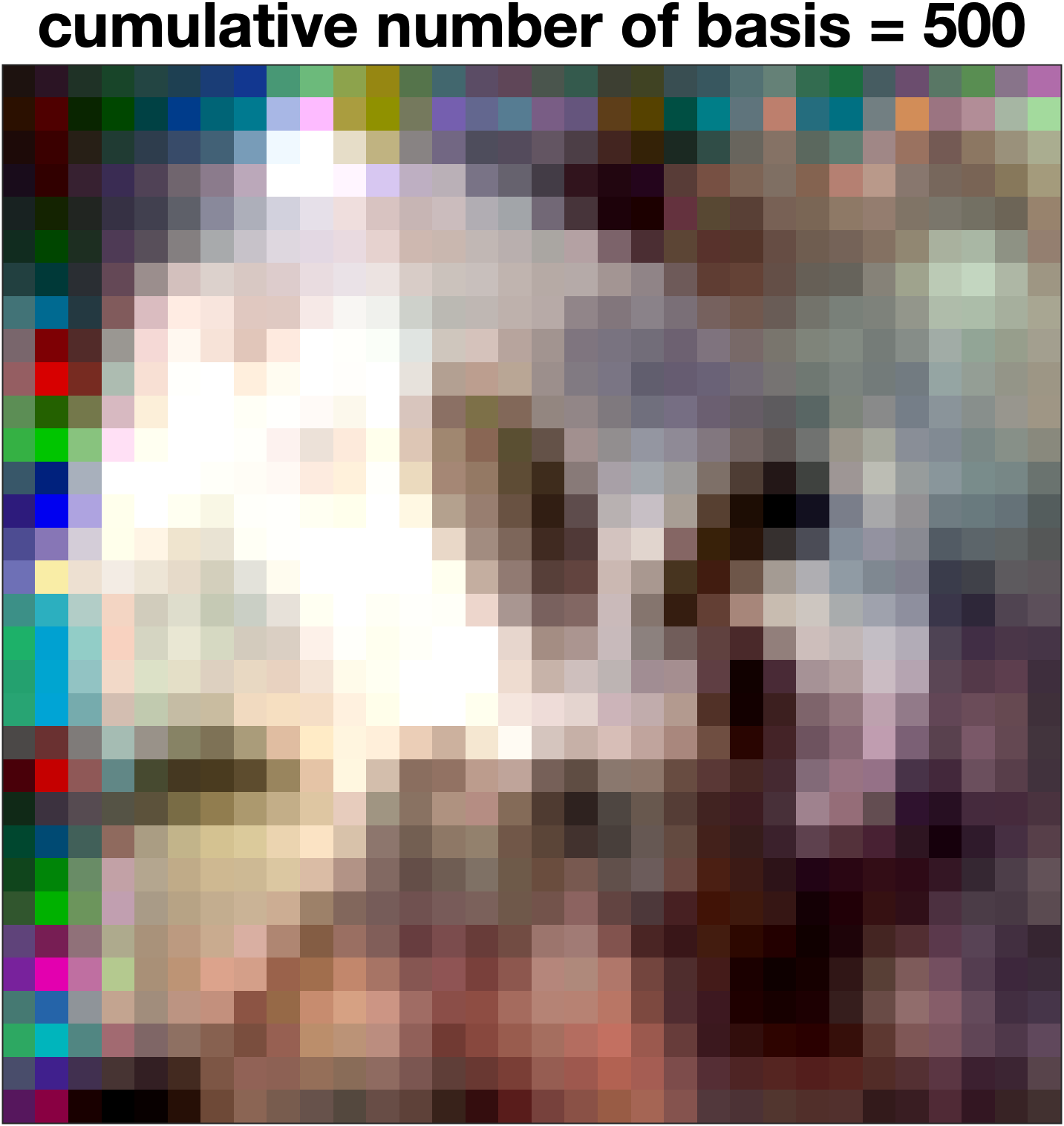
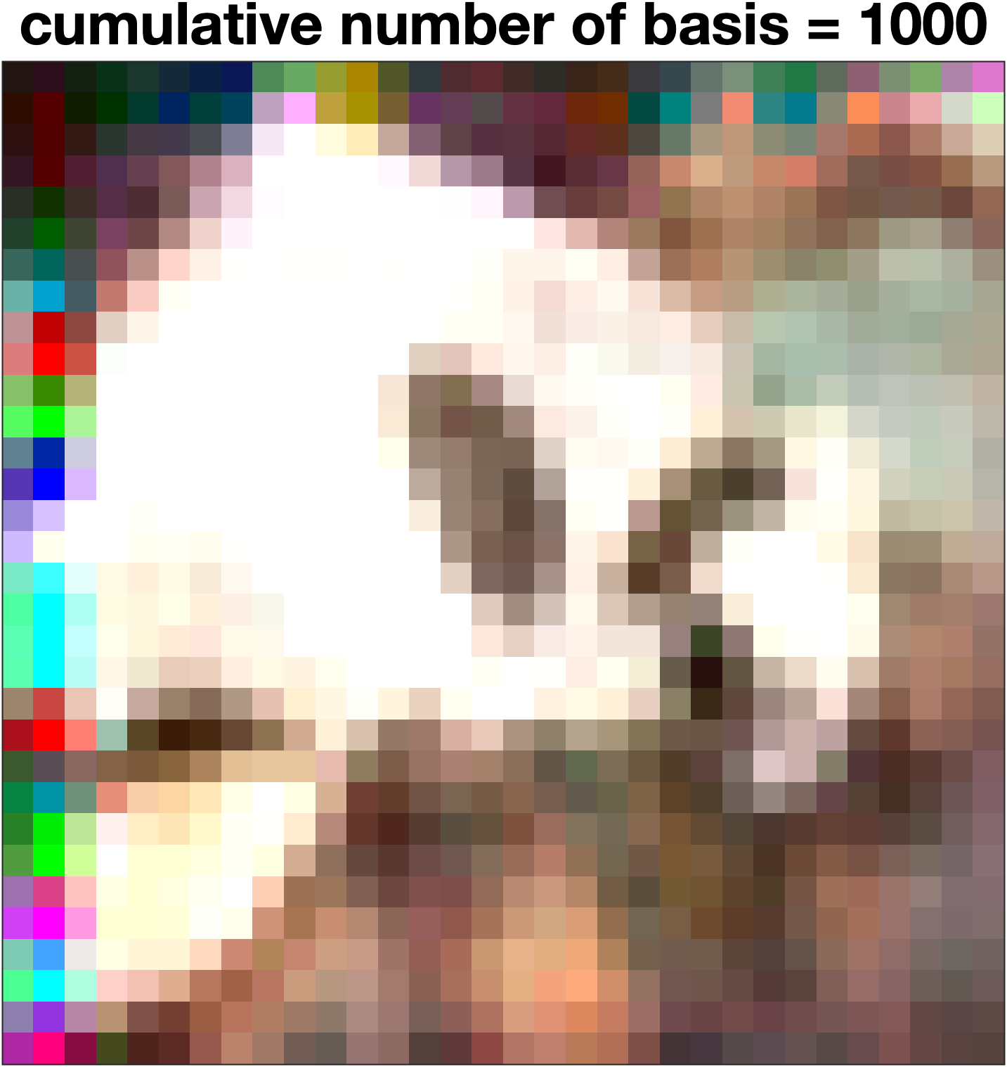
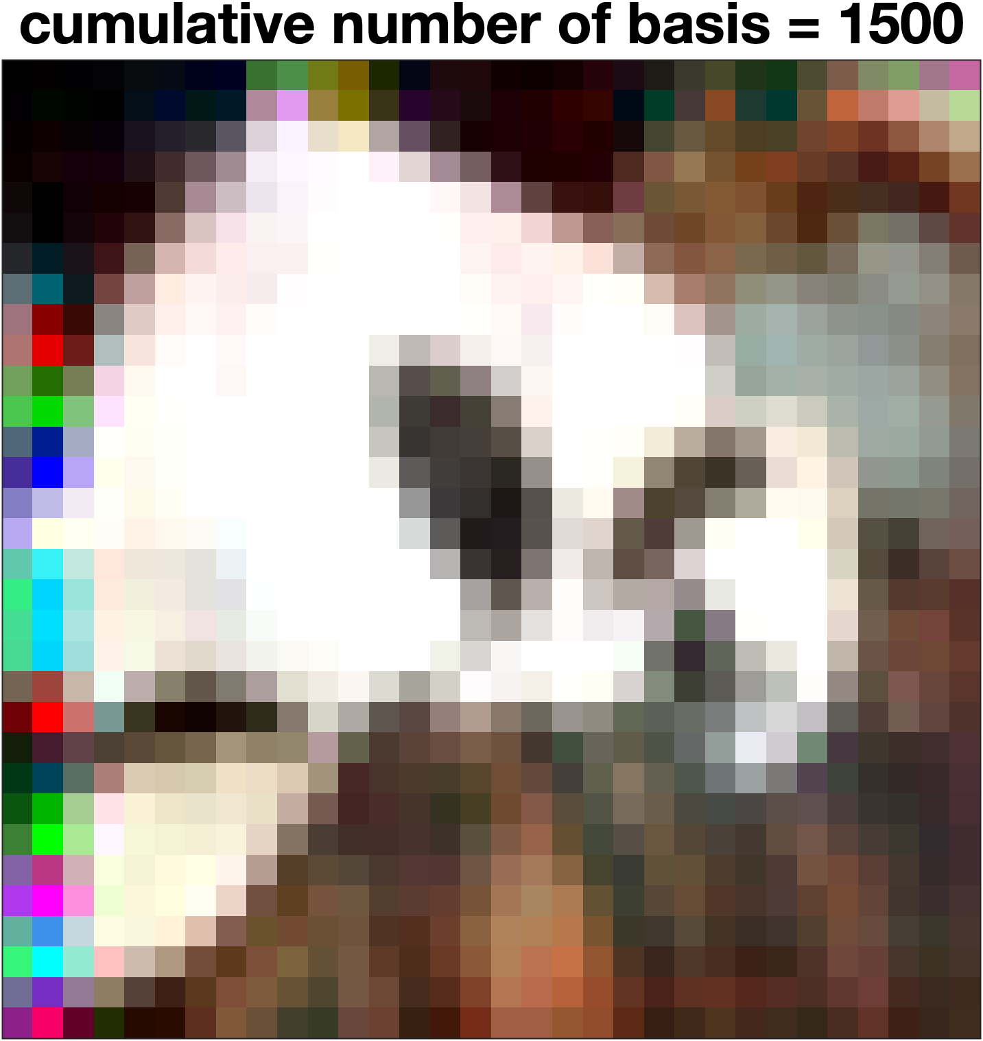
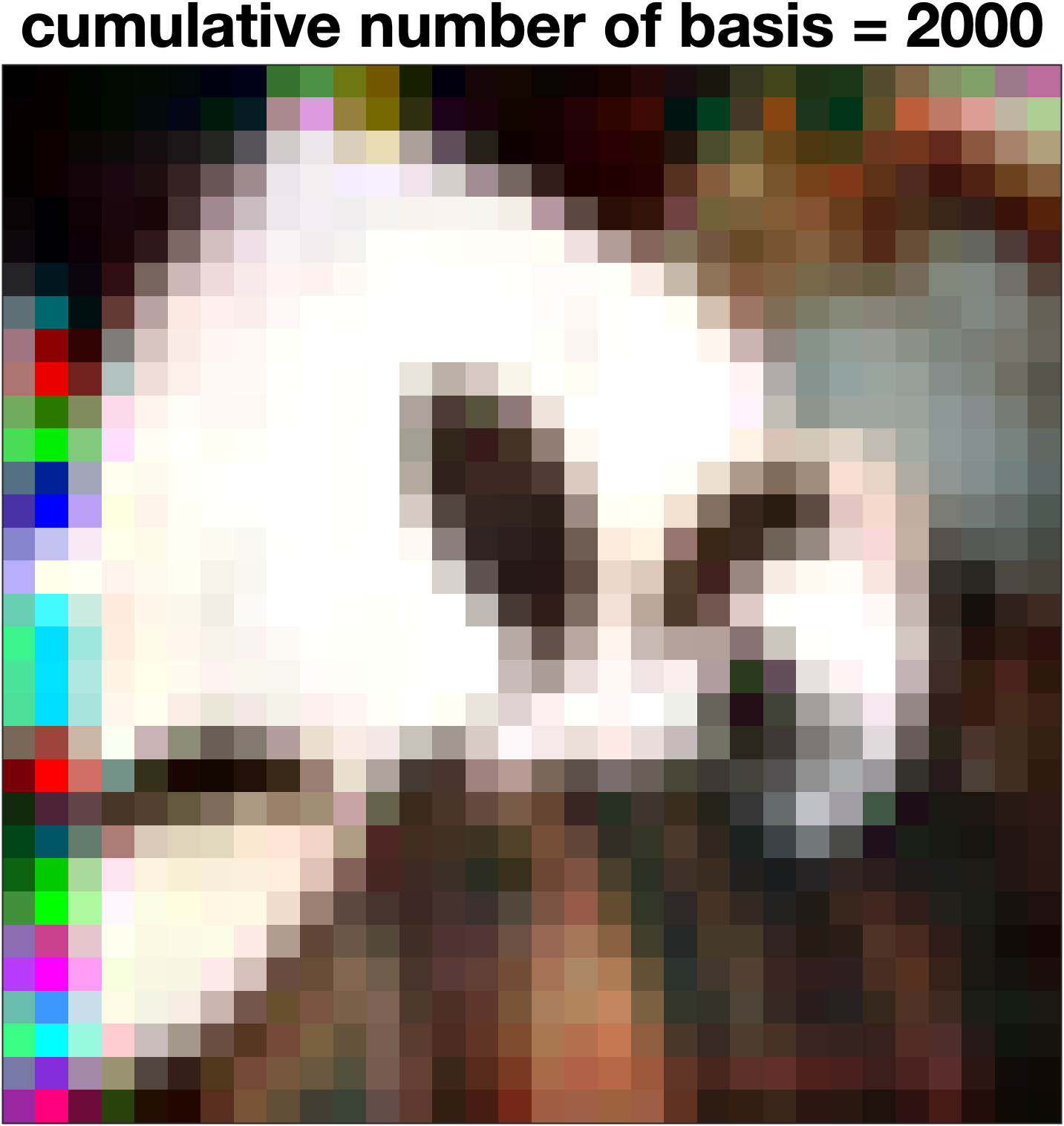
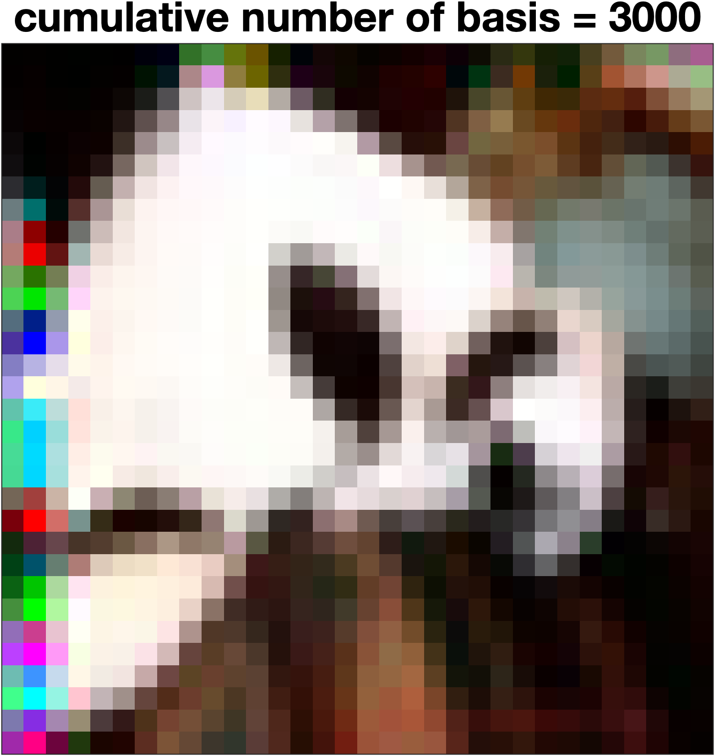
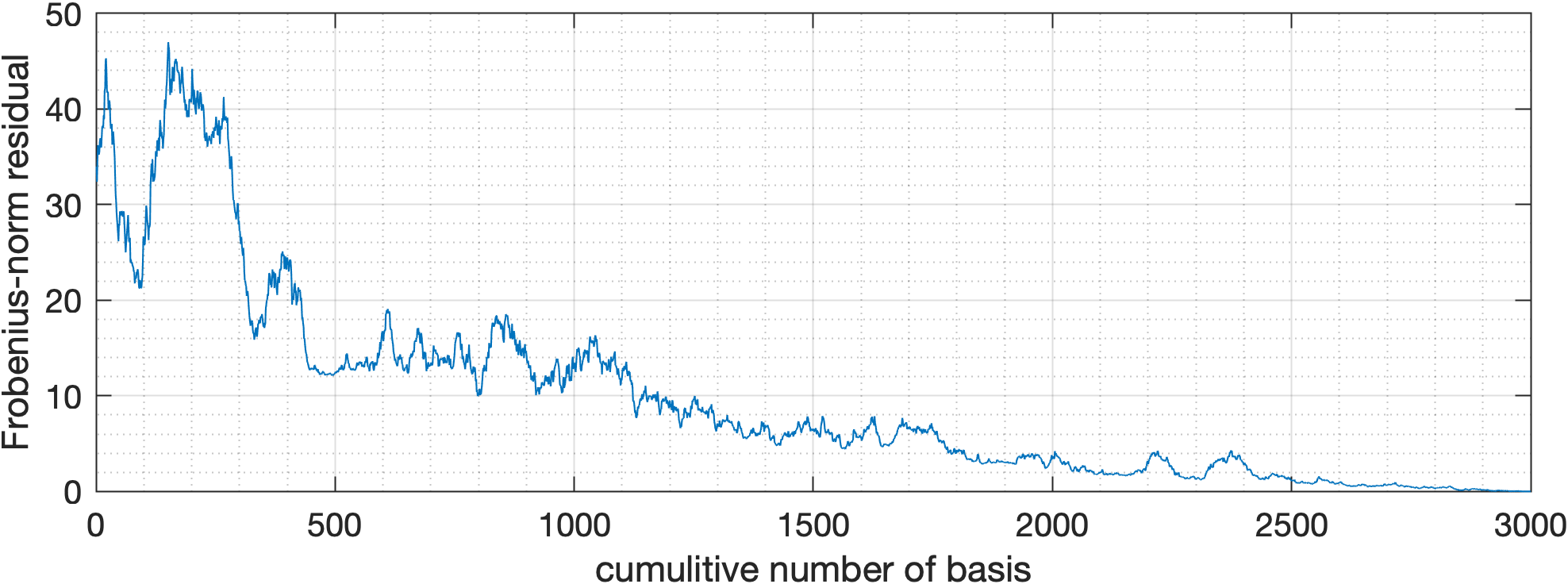
Figure B2: 331st testing image of the Cat class which is misclassified by state of art model on CIFAR-10. For this decomposition,we have used the same $V$ obtained from training set.

Appendix C Practical notes and other extensions

C.1 Practical notes about our algorithm

Our Algorithm 1, uses the parameter $\tau$ to impose an upper bound on the condition numbers of the slices of data. Since we choose the wavelet coefficients using the RR-QR algorithm, imposing the upper bound on condition numbers of the slices of the data leads to discarding the possible redundancies and rank deficiencies in the data and ensures that the remaining data is not rank deficient. As a practical value based on our numerical experiments, we recommend $\tau$ to be chosen between $10^{5}$ to $10^{7}$. Choosing much larger values might lead to rank deficiency.

Generally, choosing a smaller value for $\tau$ would lead to a smaller $m$, which means fewer wavelet coefficients are involved in our analysis, which might lead to extracting vague patterns at the end. It is important to note that when we decompose an image with a wavelet basis, we can reconstruct it perfectly (to some computational precision), if we use all the wavelet coefficients of the decomposition. If we choose only a subset of those coefficients, the reconstructed image may have a lower quality, some patterns might become blurry and vague, and some pixel values might become completely lost. Therefore, we would not want to discard too many of the wavelet coefficients by choosing the $m$ very small.

Finally, for datasets with high resolution images, it would be most efficient to first reduce the resolution of images and then perform the analysis. Some images might have pixels in the order of millions. Seeing a high-resolution image with millions of pixels is visually nice for humans, but we would not need the fine level resolution to identify patterns that distinguish one class from the others. Additionally, decomposing extremely large tensors might be computationally intractable.

C.2 Shearlets

We note that shearlets are also a multi-scale framework, similar to wavelets, which can have certain advantages in capturing edges and other an-isotropic features in images [Labate et al., 2005, Kutyniok and Labate, 2012]. For example, shearlets are used to extract features from images for edge detection [Andrade-Loarca et al., 2019, Schug et al., 2015] and image interpolation [Lakshman et al., 2015]. Investigating whether shearlets can extract more useful information and patterns from the image-classification datasets can be a future direction of research.

Appendix D Our results on MNIST

We consider all 10 classes of MNIST. To decompose the images, we choose Daubechies-1 wavelet basis. More information about the data is presented in Appendix A. We also use $m=100$ which satisfies the full rank requirement for all classes.

Patterns in the dataset. Again, we use the Higher Order GSVD as our spectral decomposition method. Figure D1 shows the images reconstructed from the first 9 columns of the right basis, $V$.

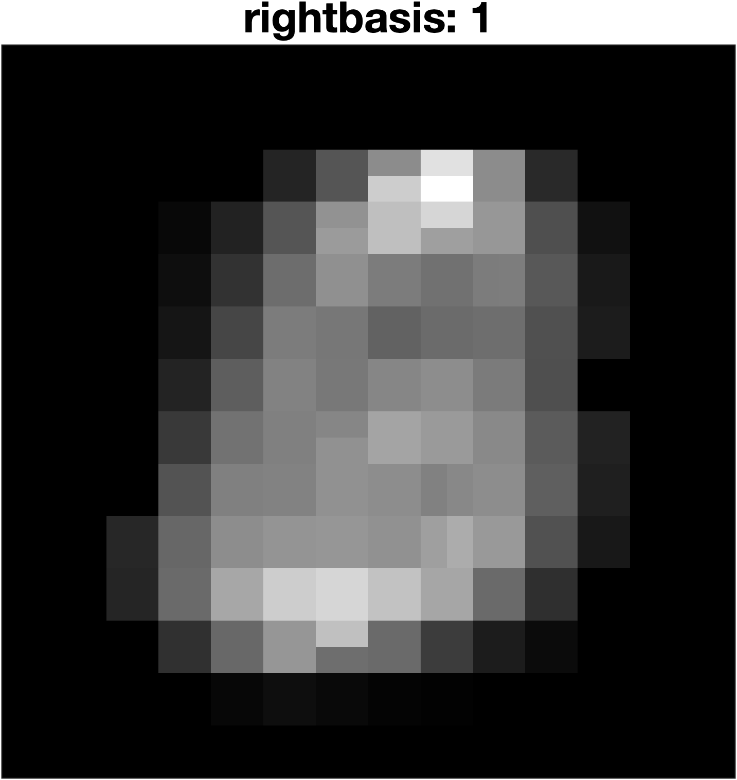
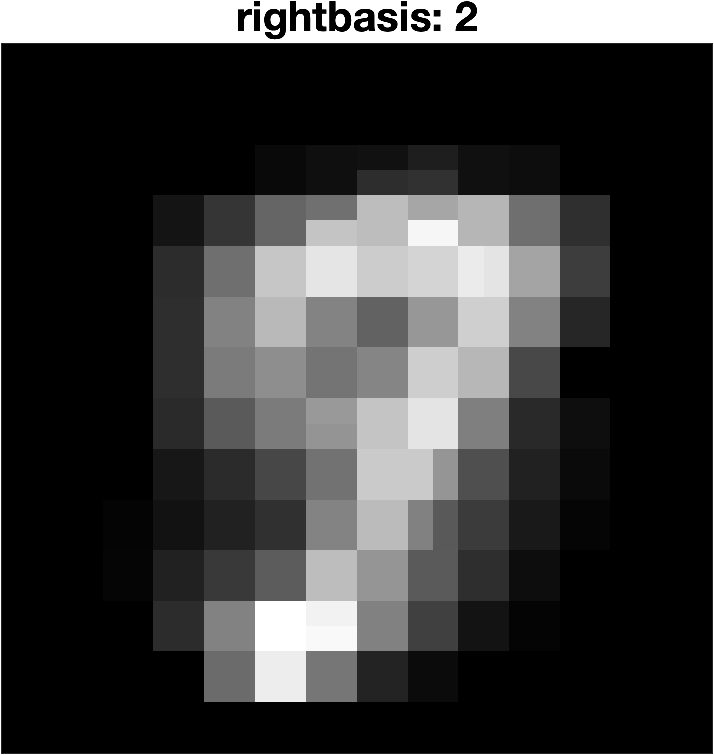
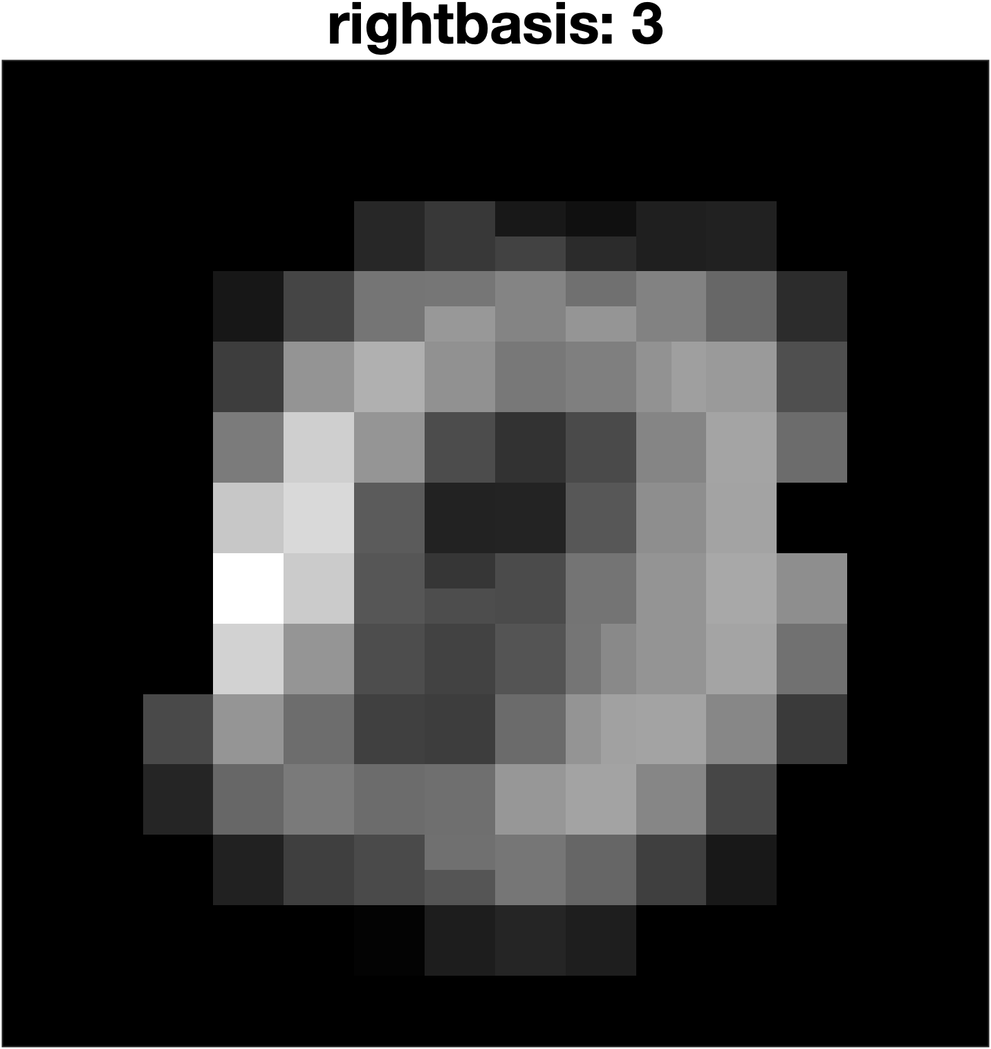
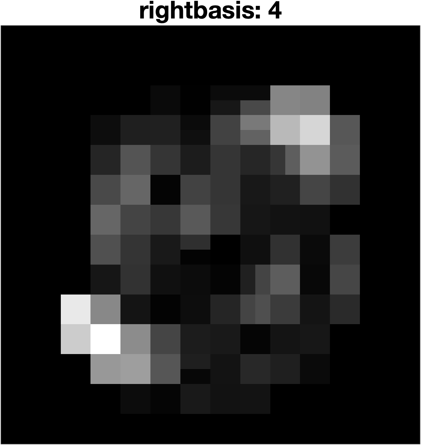
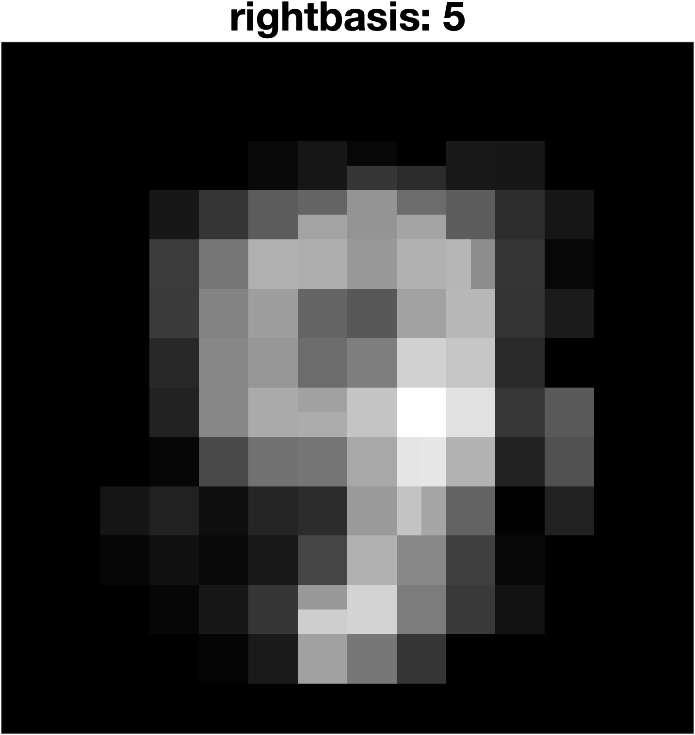
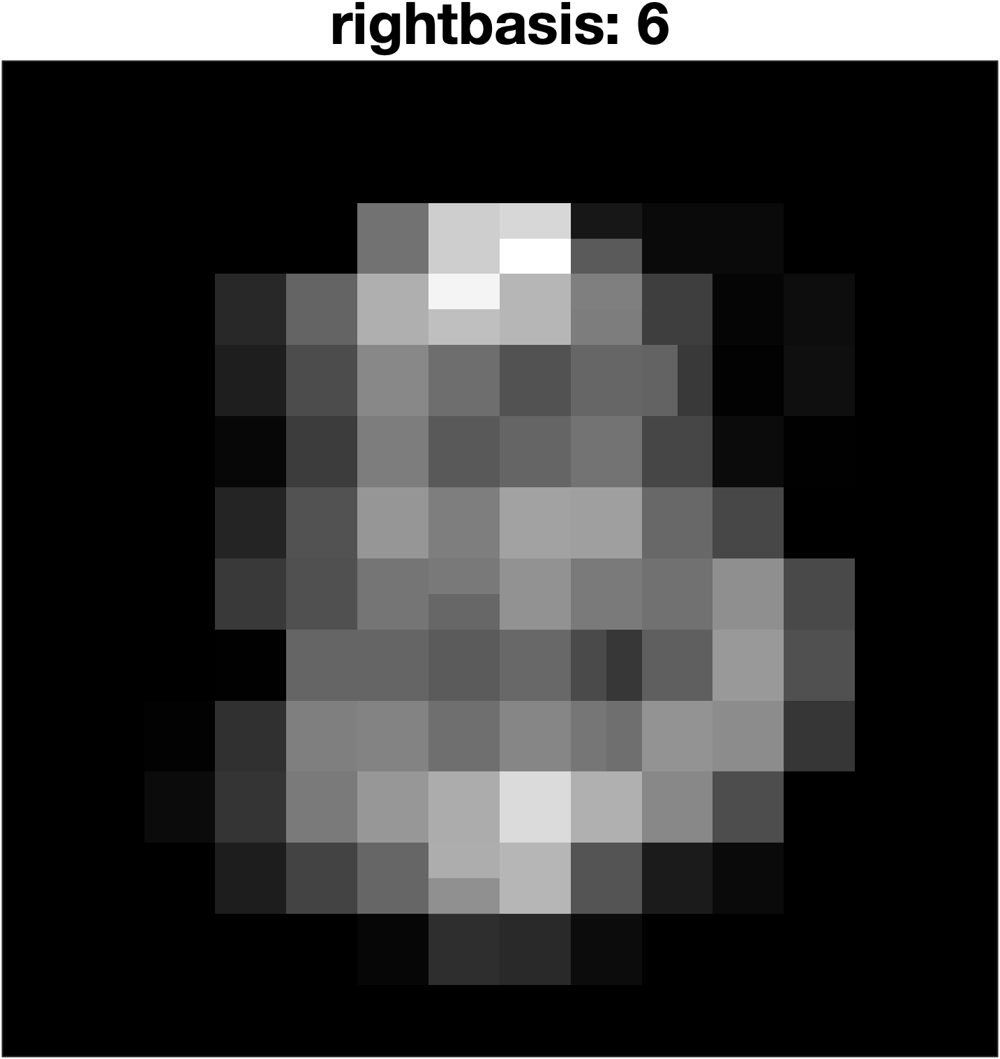
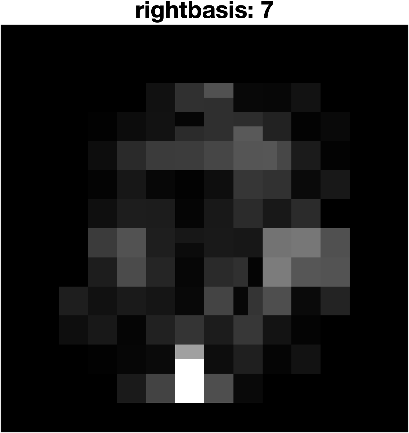
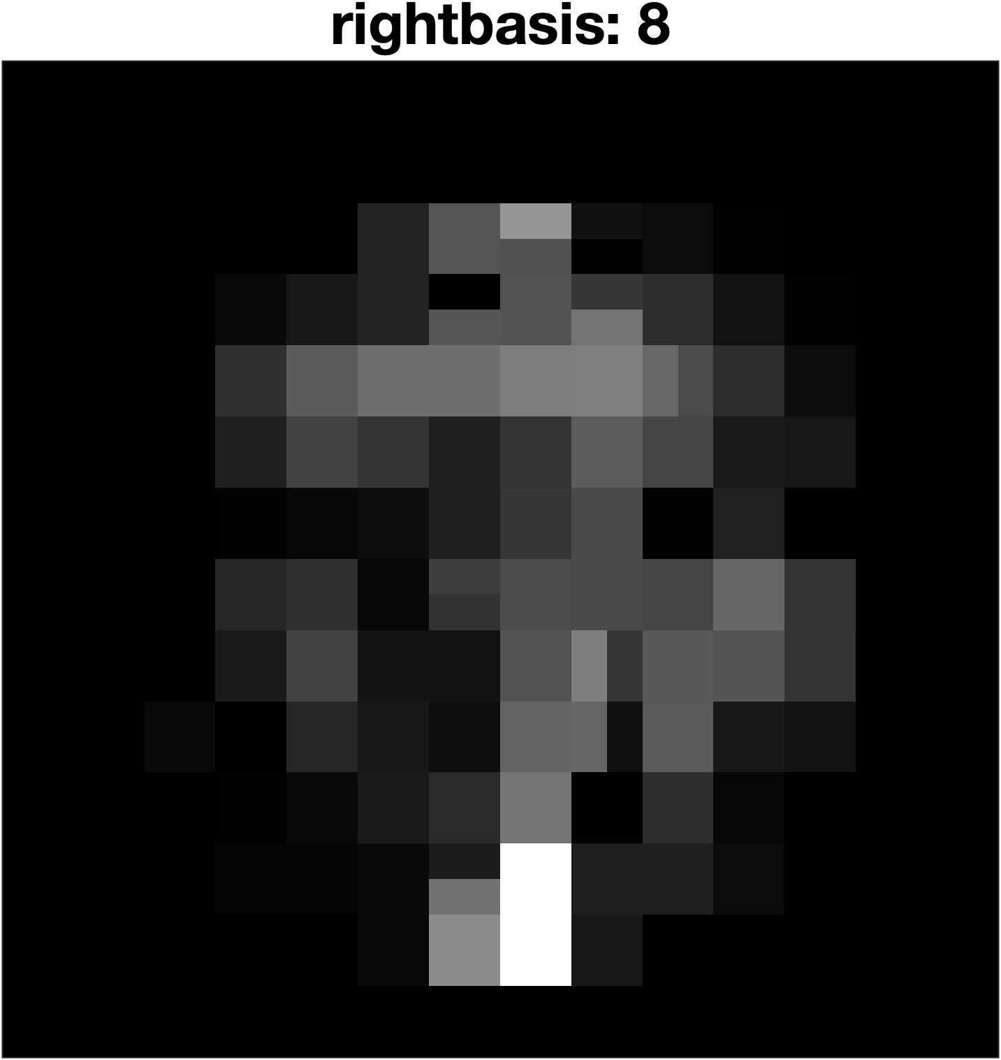
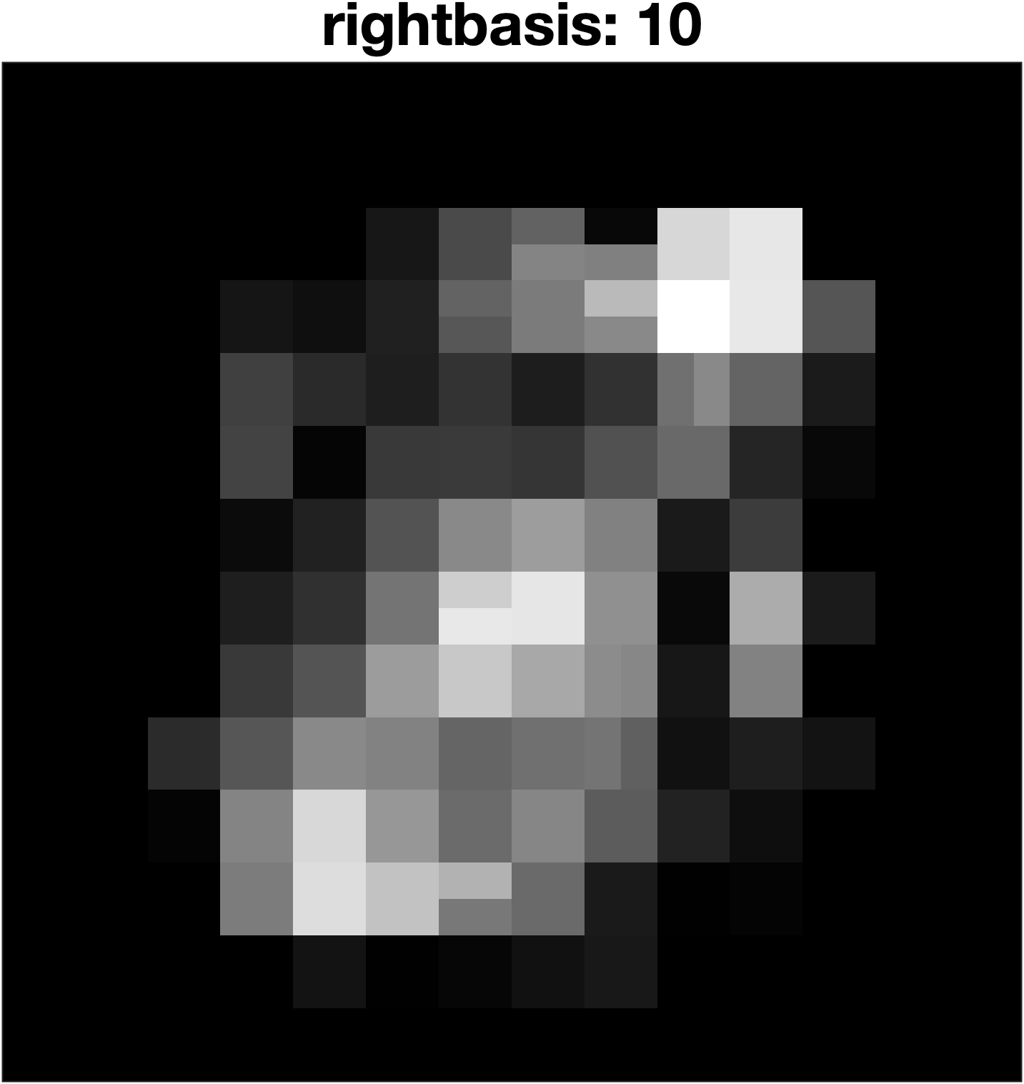
Figure D1: Images reconstructed from individual columns of the right basis $V$.

Singular values and association of patterns to classes. Figure 2(a) shows the first 20 singular values for all classes, and Figure 2(b) shows the second 20 singular values, i.e., singular values 21 through 40.

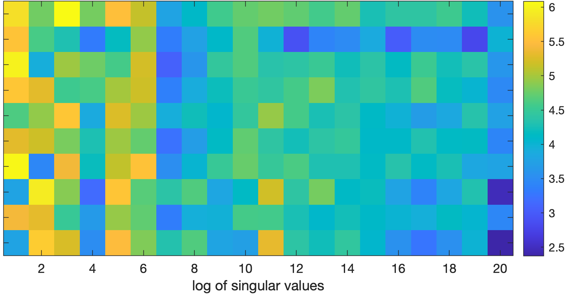
(a) Singular values 1 through 20

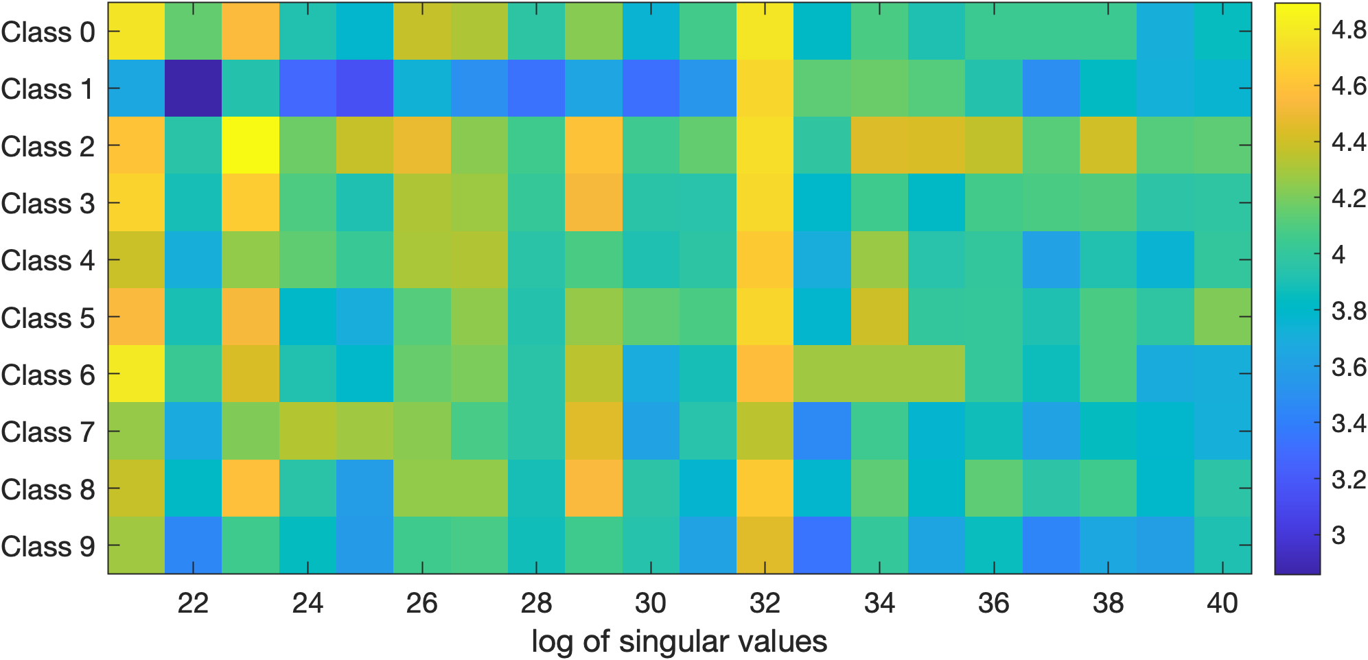
(b) Singular values 21 through 40

Figure D2: Log of singular values for all classes of MNIST. Some singular values are dominant for a particular class and some of them are dominant for more than one class.

Interpreting the patterns. Consider the images for columns 7 and 8 of right basis, reconstructed in Figure D1. One could rationalize that they represent distinctive features for classes of 4,7, and 9, because those patterns have a vertical stroke at the bottom of image and they all have some vague content at the center. Looking at the singular values (columns 7 and 8 in Figure 2(b)), reveals that the dominant singular values are exactly those digits (4, 7, and 9).

Let’s consider the 32nd singular value which seems to be relatively similar for all classes, i.e., the column 32 in Figure 2(b). The image reconstructed from the 32nd column of right basis, $V$, is shown in Figure D3 (left), which seems to be a general basis, not distinctive for any particular digit. Now, lets’ consider the 50th column in $V$ where its reconstruction is shown in Figure D3 (right). The dominant singular values for this class are classes 5 and 8, which seems to correspond to the distinctive patterns one would expect for digits 5 and 8.

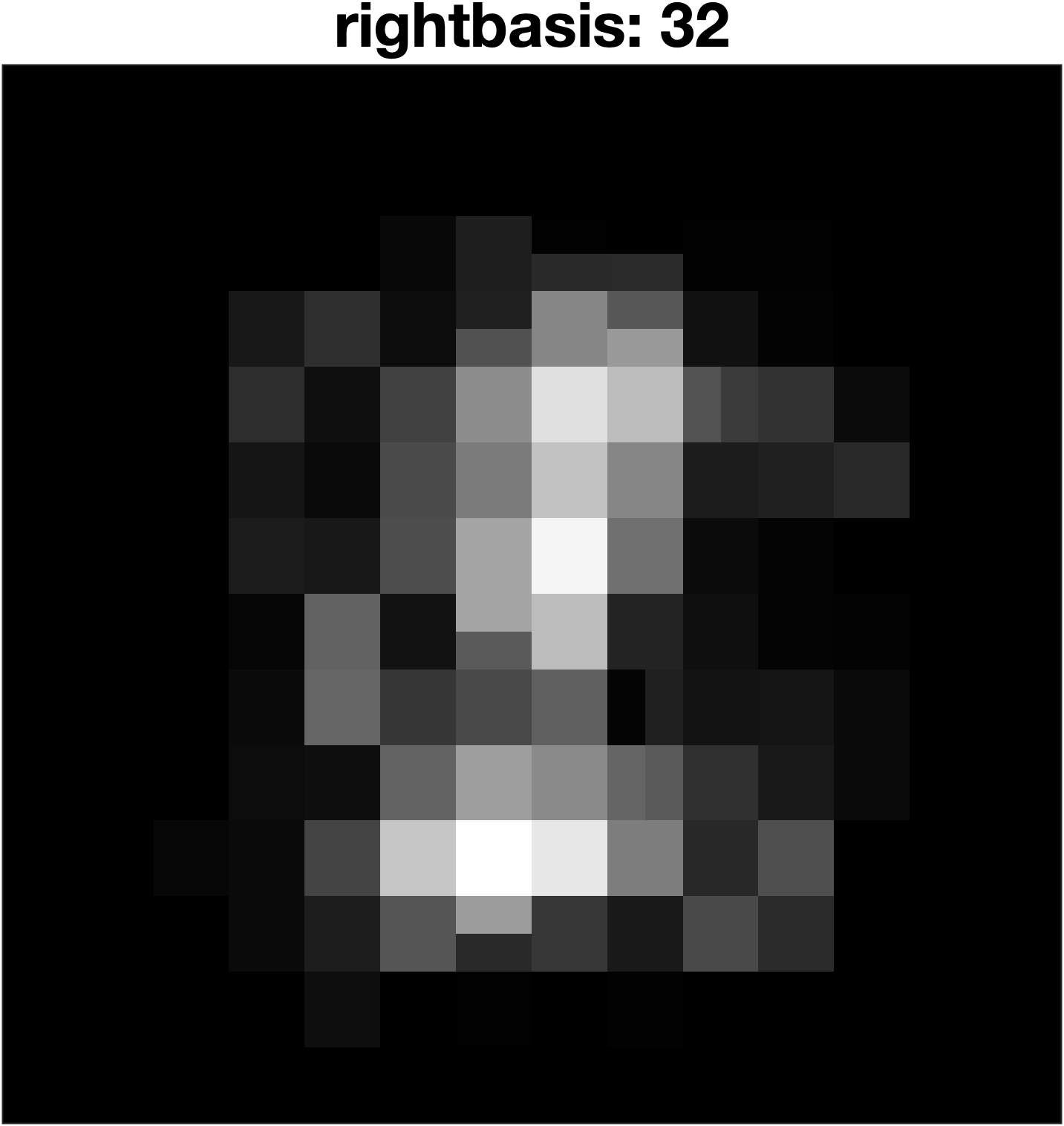
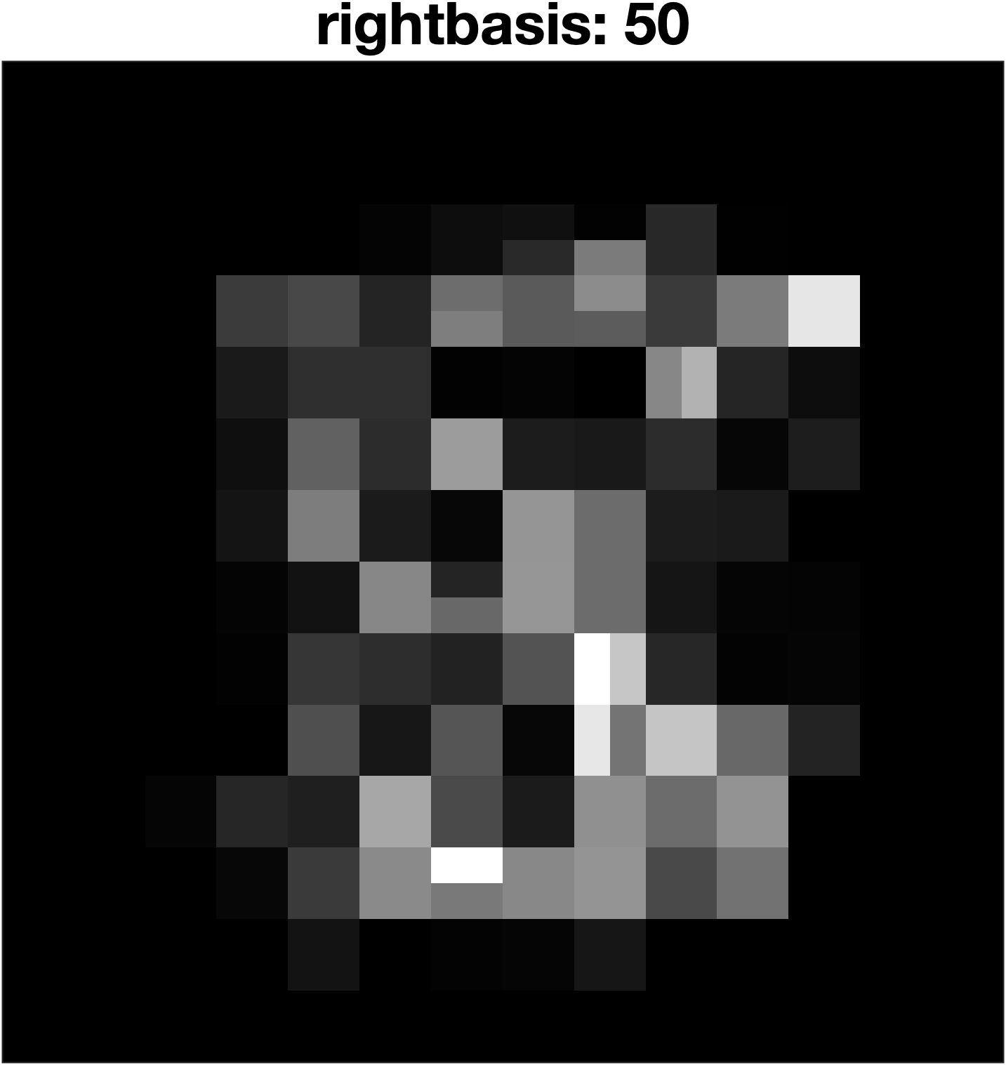
Figure D3: Images reconstructed from individual columns of the right basis $V$.

Left basis interpretation. Now, let’s consider the left basis for digit 1. The three images with the largest norm in the left basis are shown in Figure 4(a). On the other hand, the images with the smallest norm in the left basis are shown in Figure 4(b). Clearly, the simple images that one would consider straightforward to reconstruct or classify are the ones with small norm in left basis, and vice versa.

(a)

(b)

Figure D4: (a) Images that have the largest norm in left basis are made from many patterns and seem atypical. (b) Images that have a small norm in left basis are simple to reconstruct from the patterns.

Appendix E Analyzing the similarities using the left basis

Here, we take a more unsupervised approach to analyze the similarities of images and to identify isolated images present in a dataset.

Using HO-GSVD, we explained how the vectors in $V$ represent the orthogonal patterns extracted from the entire dataset. We also know that each image in the dataset can be reconstructed by a specific combination of patterns in $V$, defined by the singular values and the left basis vectors. In fact, $V$ is common among all the classes in the dataset $V$ and what distinguishes each image from other images, is its corresponding vector in $U_{i}\Sigma_{i}$. The number of rows in $U\Sigma$ correspond to the number of images in the class $i$. Let’s consider the $j^{th}$ image in class $i$. We can reconstruct this image using the coefficients in the $j^{th}$ row of $U_{i}\Sigma_{i}$ to combine the vectors of $V$. Mathematically, if we have two identical images in the dataset, we will get identical coefficients for them.

Overall, we can say that the HO-GSVD extracts a set of common patterns in the entire dataset, and gives us a set of coefficients in $U_{i}\Sigma_{i}$, determining how these patterns should be combined in order to obtain the images. To analyze the similarity of images, we can analyze the similarity of their coefficients, because patterns are common for all of them. In fact, patterns can be considered images in the pixel space, but coefficients are just a vector of real numbers. This way, analyzing the similarity of two images is reduced to basically comparing two vectors.

Figure E1 shows the similarity matrix of all images in the Cat class. To derive this similarity matrix, we followed these steps:

1. Compute the matrix $U_{i}\Sigma_{i}$ which has 5,000 rows and 3,000 columns for the Cat class.

2. Compute the 2-norm distance between each row in this matrix to obtain a distance matrix of 5,000 rows and columns.

3. Convolve the distance matrix with a Gaussian kernel to obtain the similarity matrix.

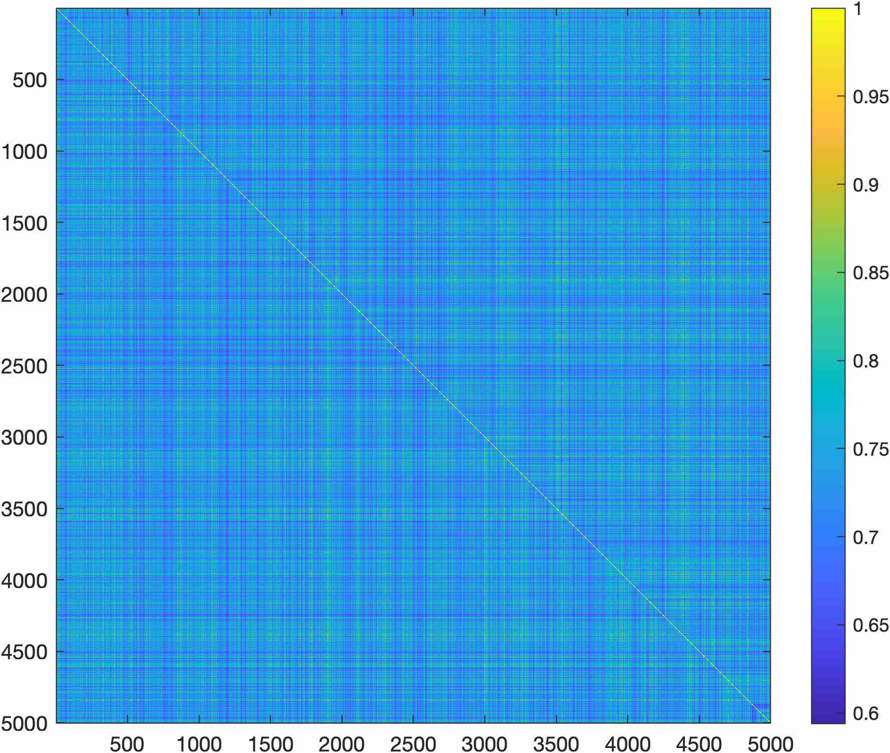
Figure E1: Similarity matrix of images in the Cat class based on the coefficients in $U\Sigma$.

Once we obtain a similarity matrix, a wide array of analysis can be performed. For example, one can perform clustering to identify communities of similar images. By analyzing the eigenvalues of a graph Laplacian built from the similarity matrix, we identified that there are not any large communities inside this dataset, as previously reported by Yousefzadeh [2020]. However, coarse graining (i.e., organizing the data in large number of clusters) can easily identify small groups of images (usually 2 to 5) that are very similar, and sometimes nearly identical.

Figure E2 shows dog images that are most isolated within the dog class. Clearly, we may consider them anomalies or out-of distribution images in the context of this dataset, because picture of a dog with a red bucket on its head, or picture of a dog with red flowers around the perimeter of image are not common. This relates to the broad literature on detecting out-of-distribution images and anomalies in image classification datasets, e.g., Liang et al. [2018], Huang et al. [2019], Ren et al. [2019]. This is another possible extension of our method.

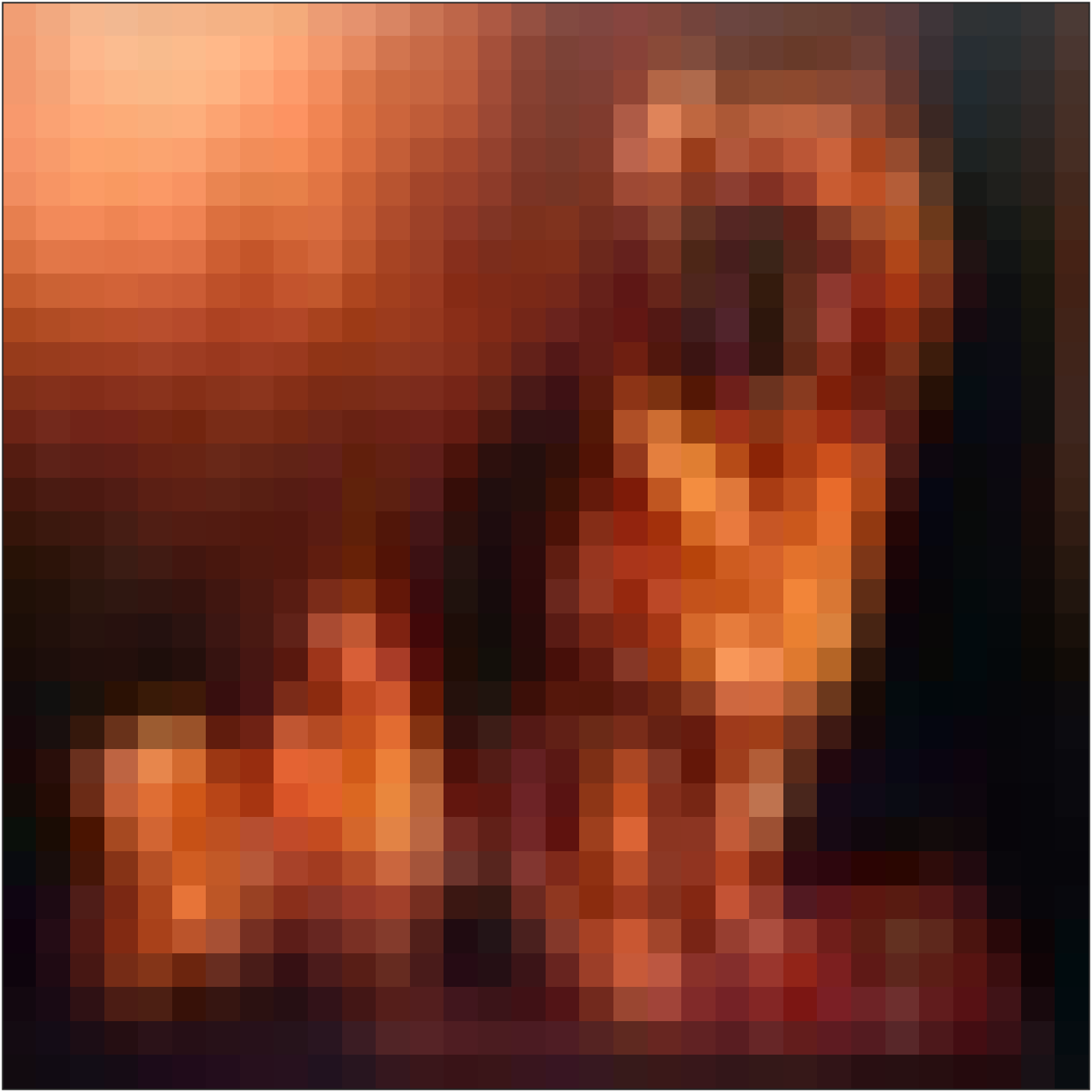
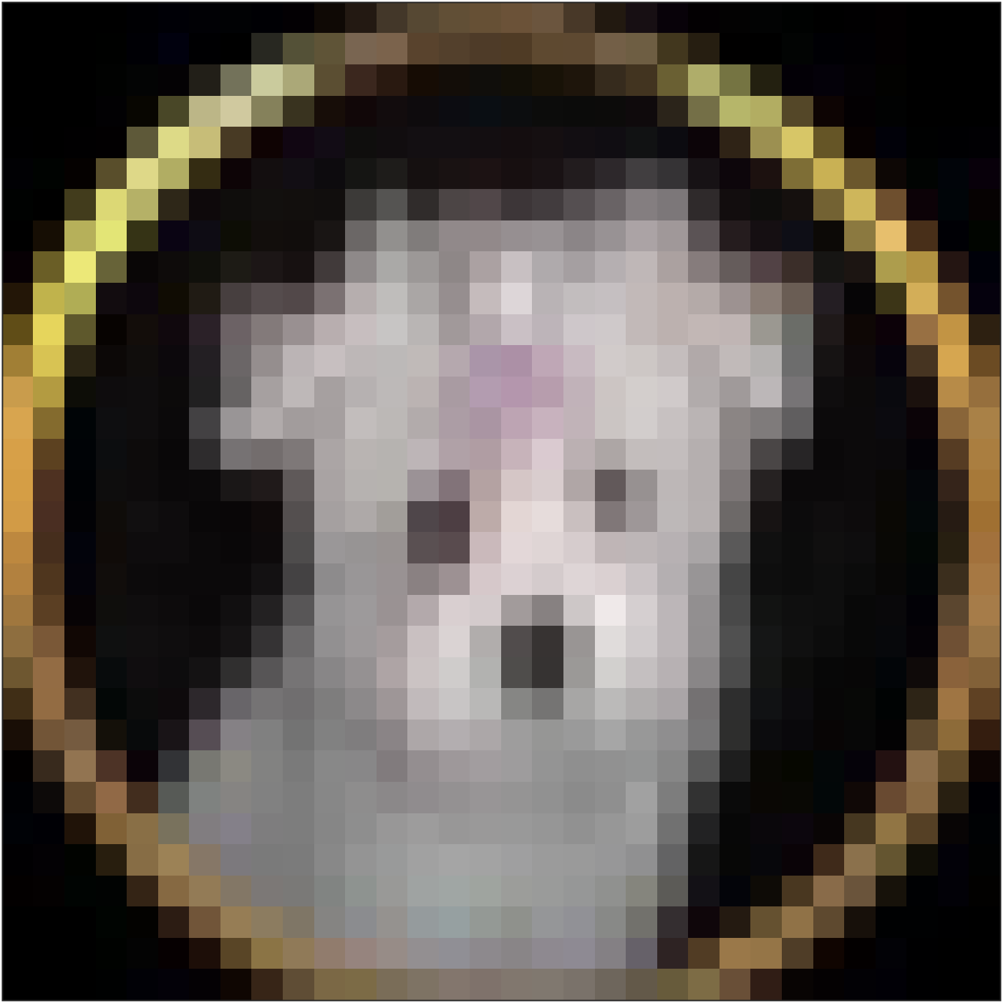
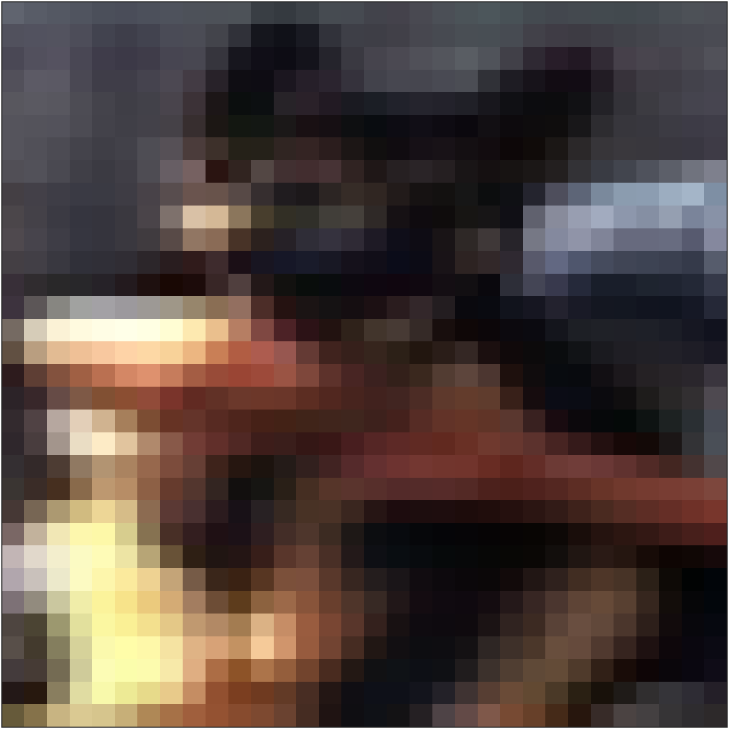
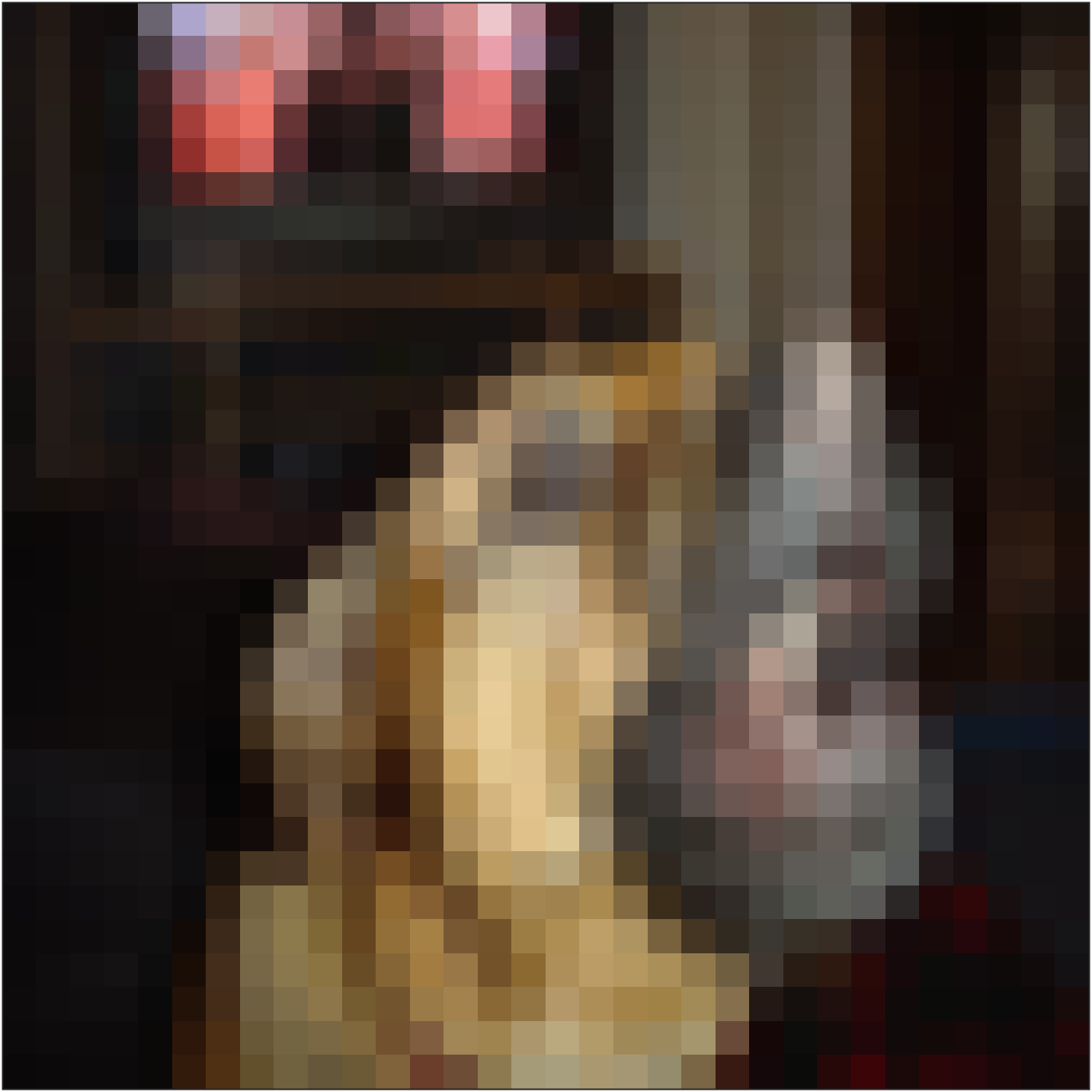
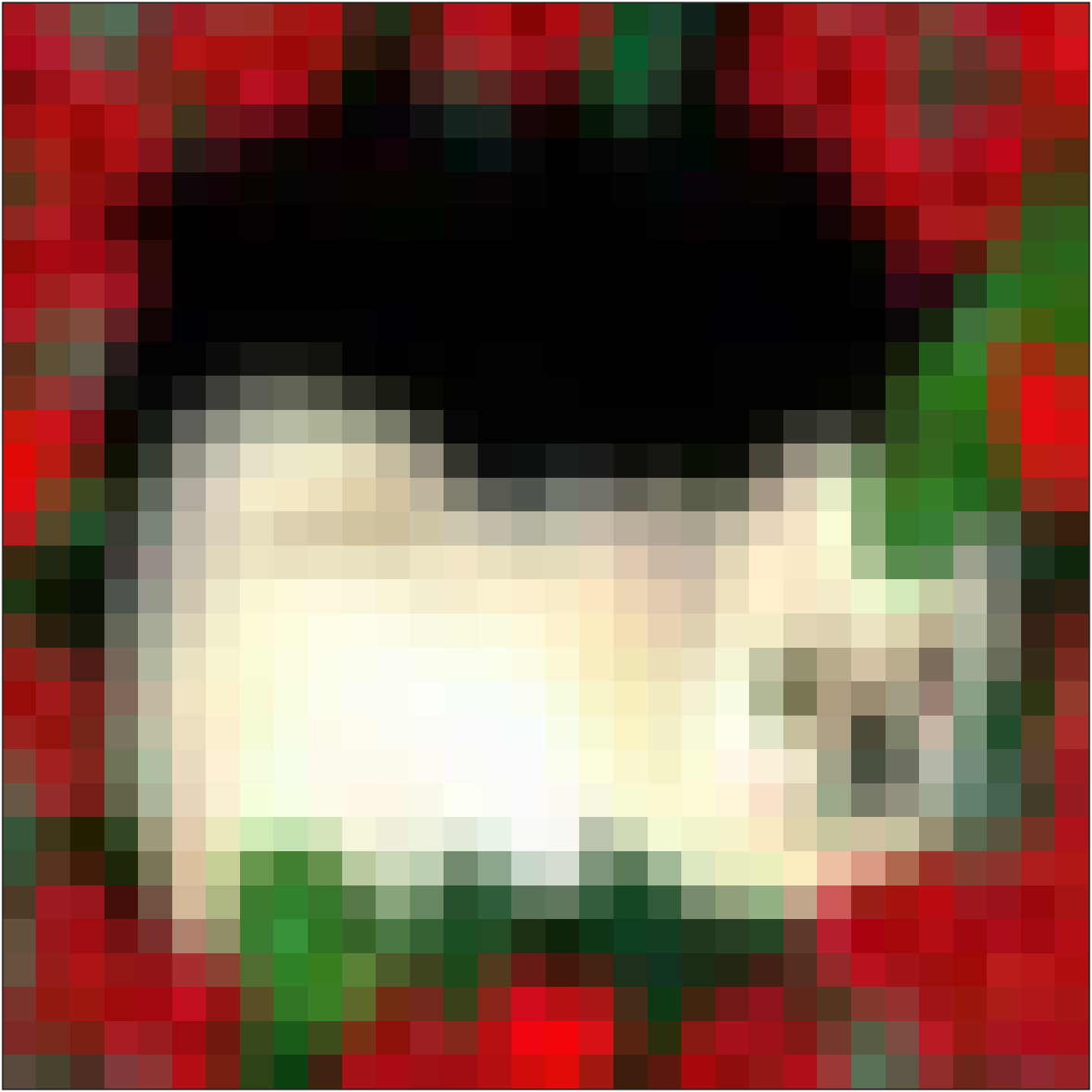
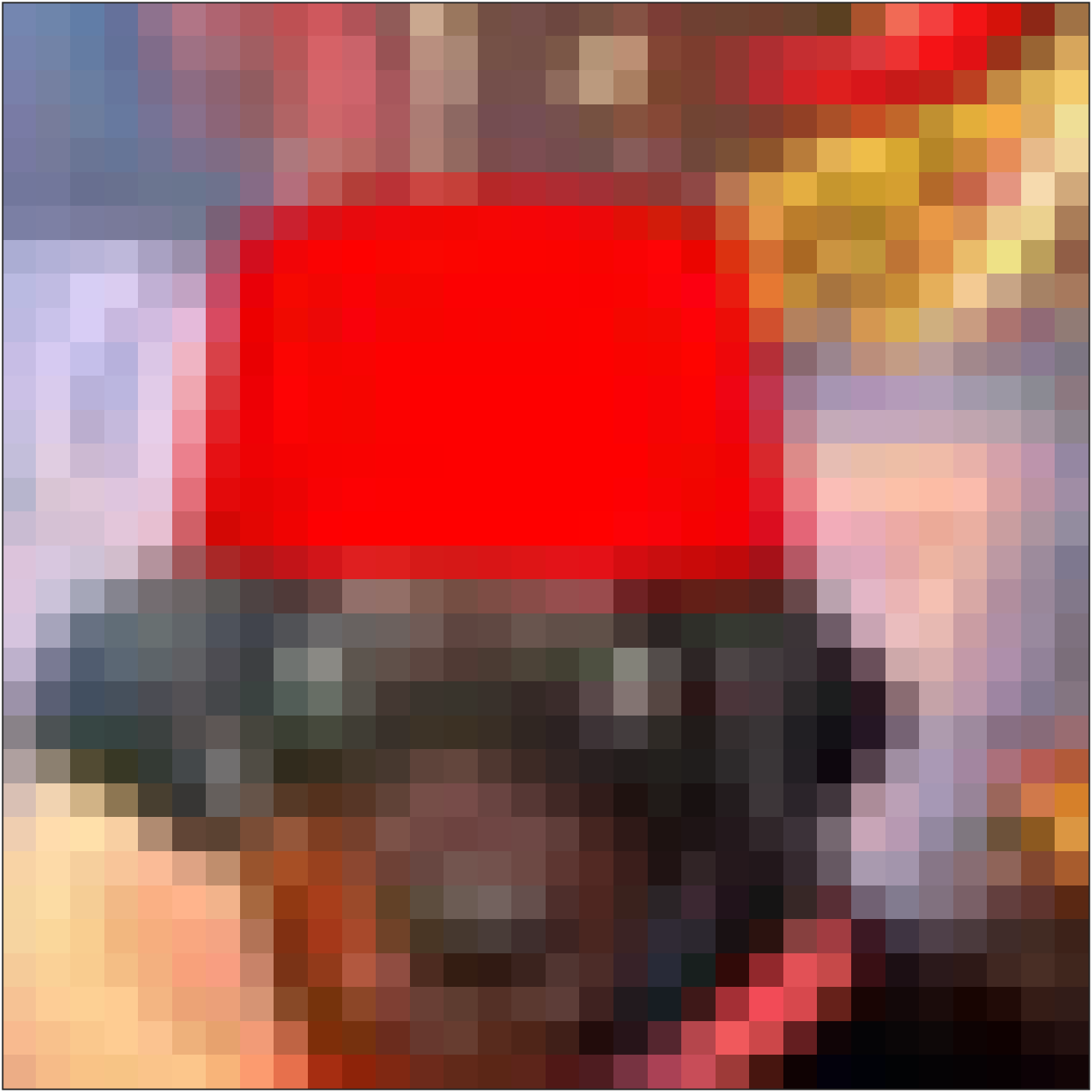
Figure E2: Dog images that are most isolated within the dog class, identified by the similarity matrix. We can consider these out-of-distribution images in the context of CIFAR-10 training set.

We can also use the coefficients in $U_{i}\Sigma_{i}$ to visualize the dataset in form of an embedding. Figure E3 shows the embedding obtained by the t-SNE (t-Distributed Stochastic Neighbor Embedding) algorithm [Maaten and Hinton, 2008]. t-SNE is a dimensionality reduction algorithm, specifically designed for visualizing high dimensional data.

This approach of visualizing a set of images in form of an embedding relates to a separate line of research in the literature. Those methods usually suffer from very high computational costs, because they rely on pairwise comparison of images in the pixel space, e.g., Vo et al. [2019]. We also note that t-SNE is used before for visualizing image datasets, for example by Parde et al. [2017], but such approaches use a pre-trained VGG model for comparison of images. Our approach does not require a pre-trained model, however, we note that its usefulness requires further experiments and comparison with other methods.

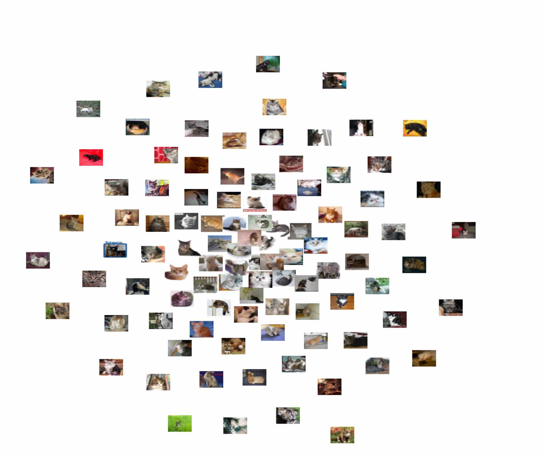
Figure E3: t-SNE plot obtained from the $U_{i}\Sigma_{i}$ matrix of cat images.

Appendix F COVID-19 CT-Scan Images

Here, we analyze the contents of the SARS-COV-2 CT-Scan Dataset [Angelov and Almeida Soares, 2020]. This dataset contains 2,482 images of CT-Scan, 1,230 of which belong to infected patients and 1,252 belong to non-infected patients. Figure F1 shows some samples from this dataset.

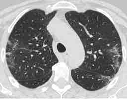
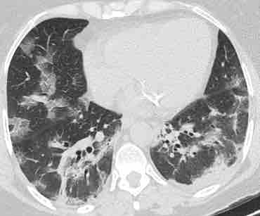
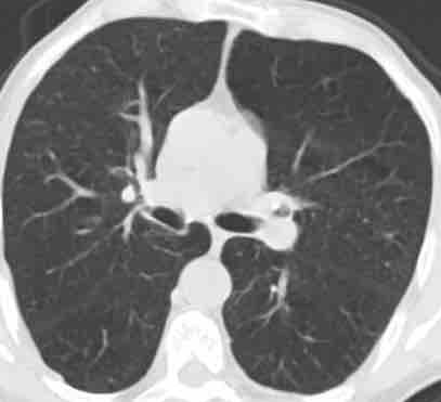
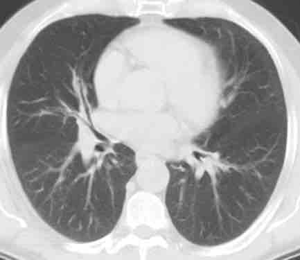
Figure F1: Sample of images in the SARS-COV-2 CT-Scan dataset. Two images in the left box are from infected patients and the ones in the right box are from non-infected patients.

We form the data into two matrices, $\mathcal{D}_{1}$ for COVID samples and $\mathcal{D}_{2}$ for non-COVID samples. For wavelet transformation, we use Daubechies-3 wavelets. We use the RR-QR algorithm to choose a subset of $m=1200$ most influential wavelet coefficients. Figure F2 highlights the pixels corresponding to those wavelet coefficients.

Figure F2: Pixels corresponding to the most influential coefficients chosen by the RR-QR algorithm. A radiologist could verify whether the patterns corresponding to infections are expected to be in those regions. RR-QR detects that most of the variations among images are in the white regions, and changes in the black regions are either small or linearly dependent.

Using Higher Order GSVD, we decompose the tensor of wavelet coefficients $\mathcal{D}$. The resulting singular values, shown in Figure F3 show a clear separation between the Covid and non-Covid patients.

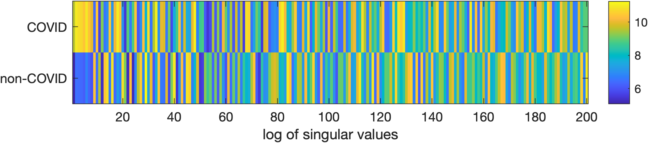
Figure F3: First 200 singular values (in logarithmic scale) show a clear separation between many of the patterns in COVID and non-COVID patients. Nitoce that when singular values are large for the COVID class, singular values are usually small for the non-COVID class, and vice versa.

Figure F4 shows the most dominant patterns obtained for the COVID patients and Figure F5 shows the most dominant patterns obtained for non-COVID patients. Clearly patterns seem very different for non-COVID and COVID patients.

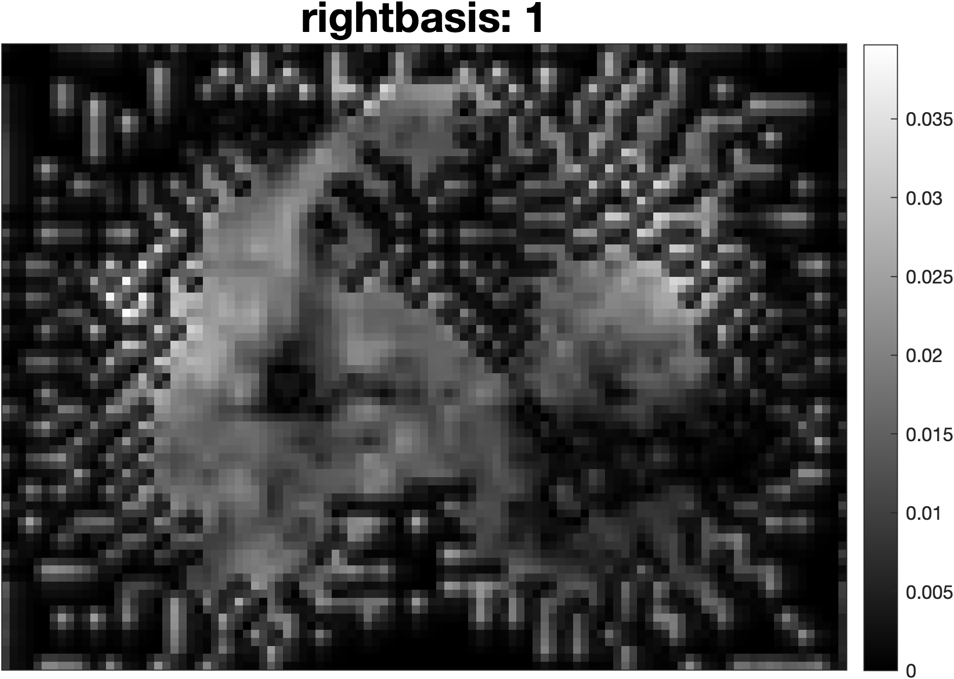
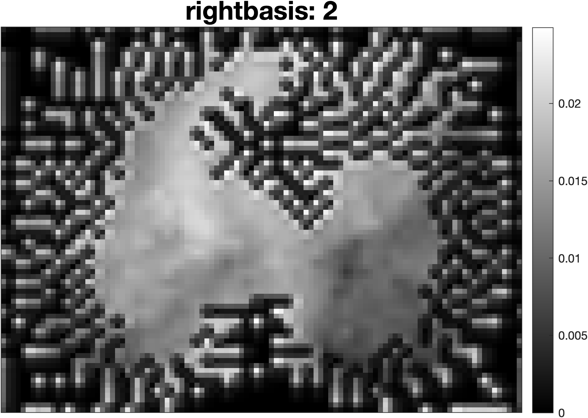
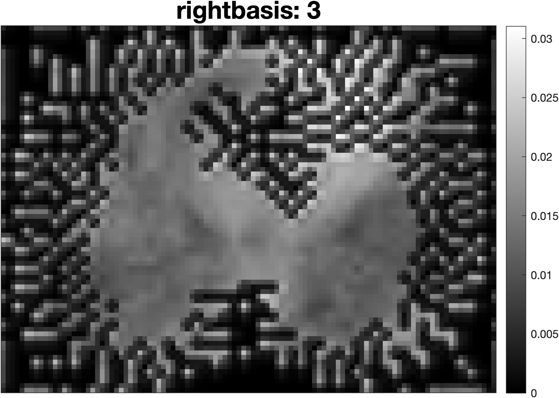
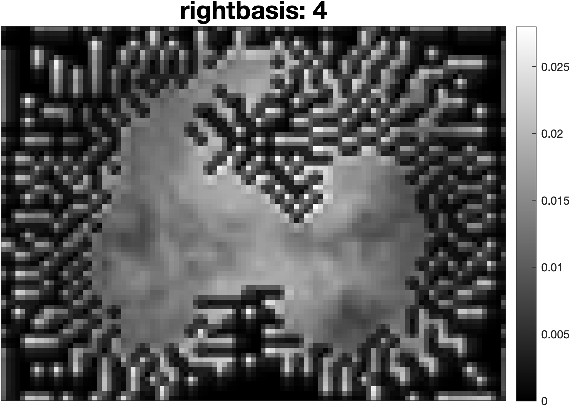
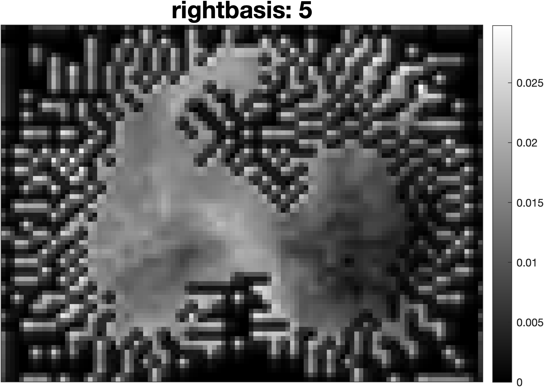
Figure F4: The most dominant patterns for COVID infected patients. Notice the color variations within the boundaries defined in Figure F2.

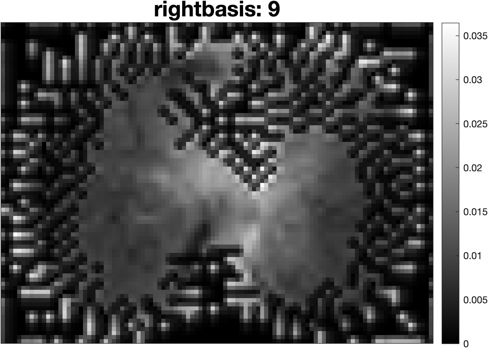
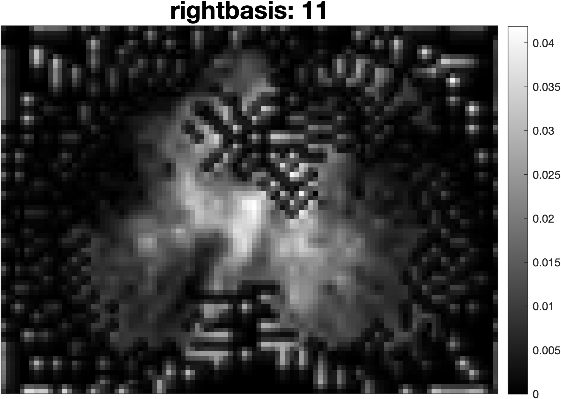
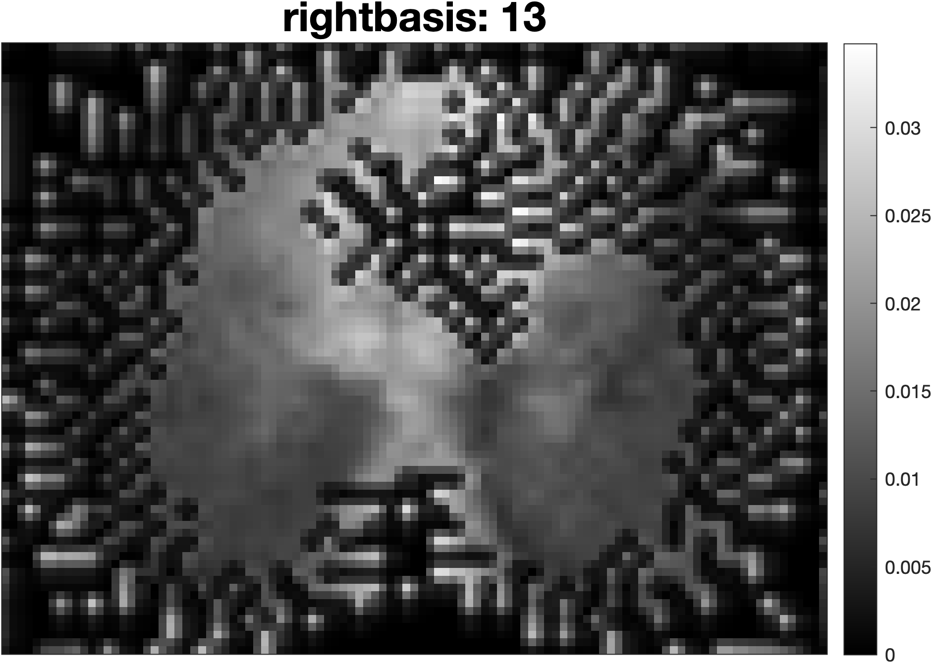
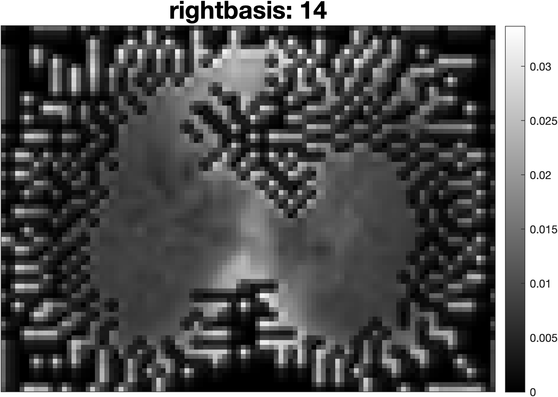
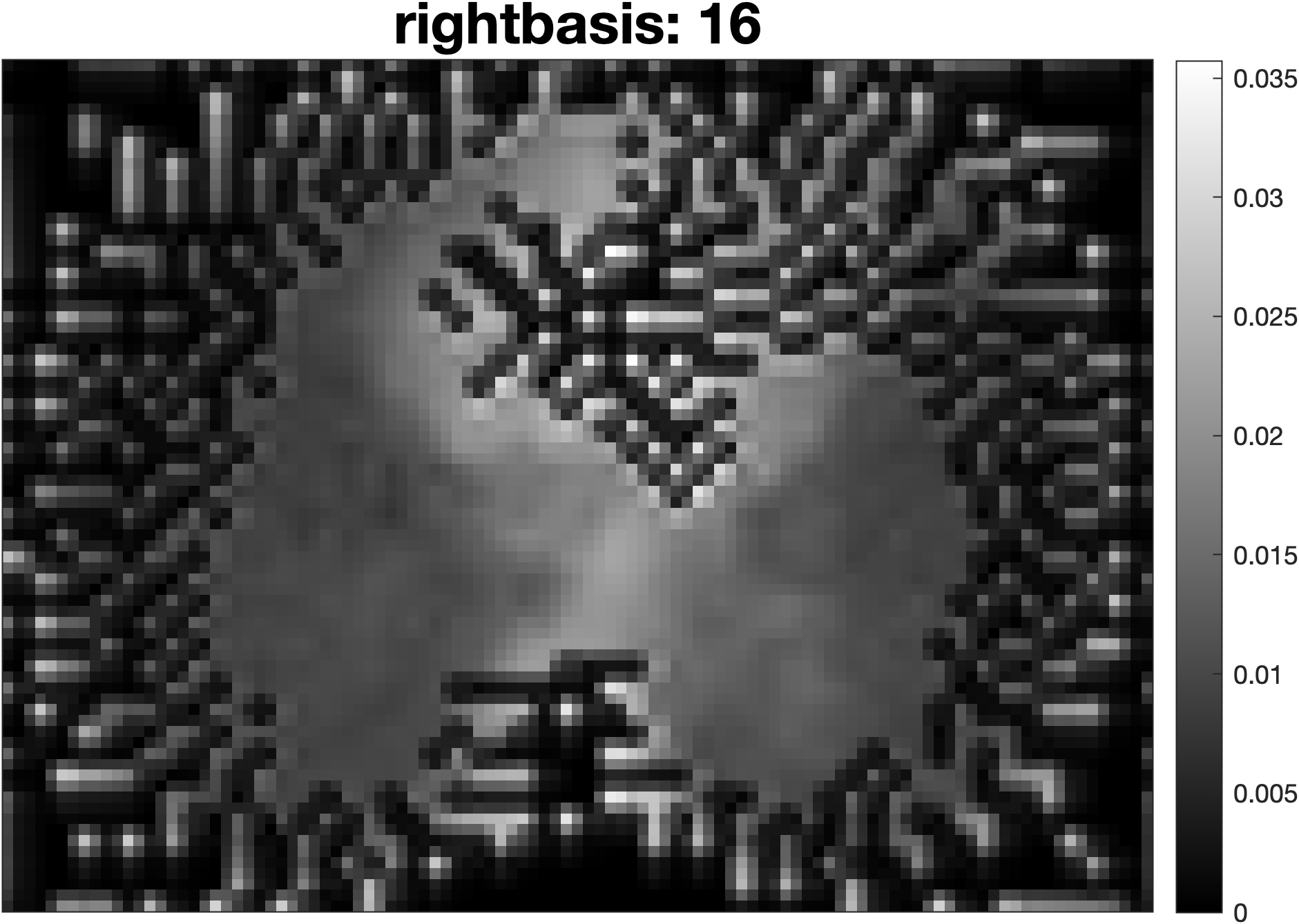
Figure F5: The most dominant patterns for non-COVID patients. Notice the color variations within the boundaries defined in Figure F2. Also, notice how the color variations are different from the COVID-19 infected patients in Figure F2.

We can use these patterns to reconstruct an image. Figure F6 shows reconstruction of an image using low-rank approximation defined by Equation 4.

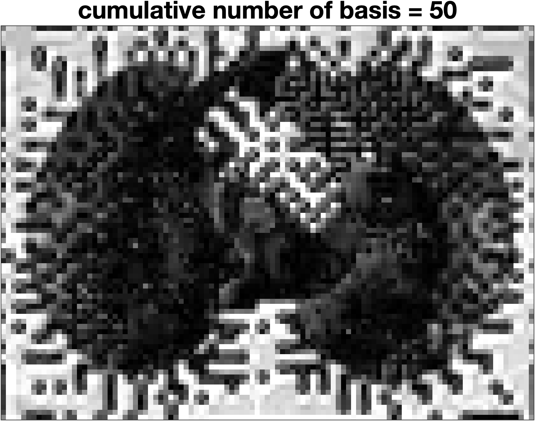
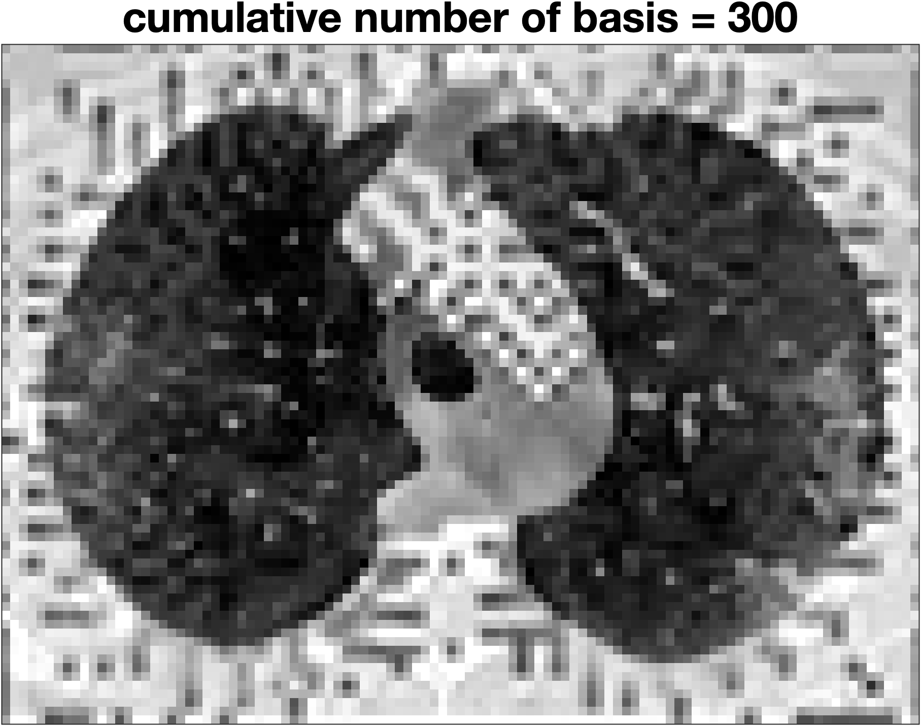
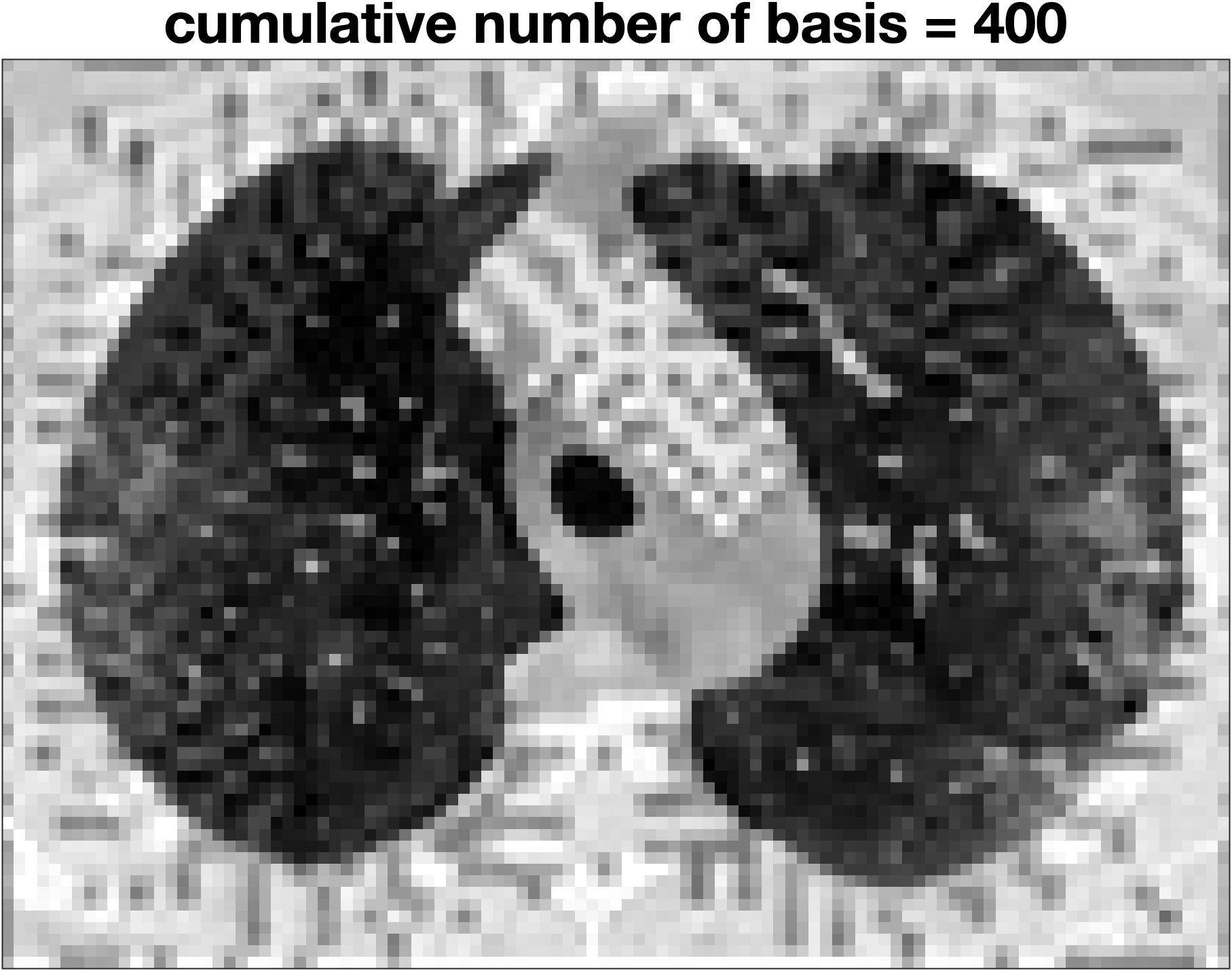
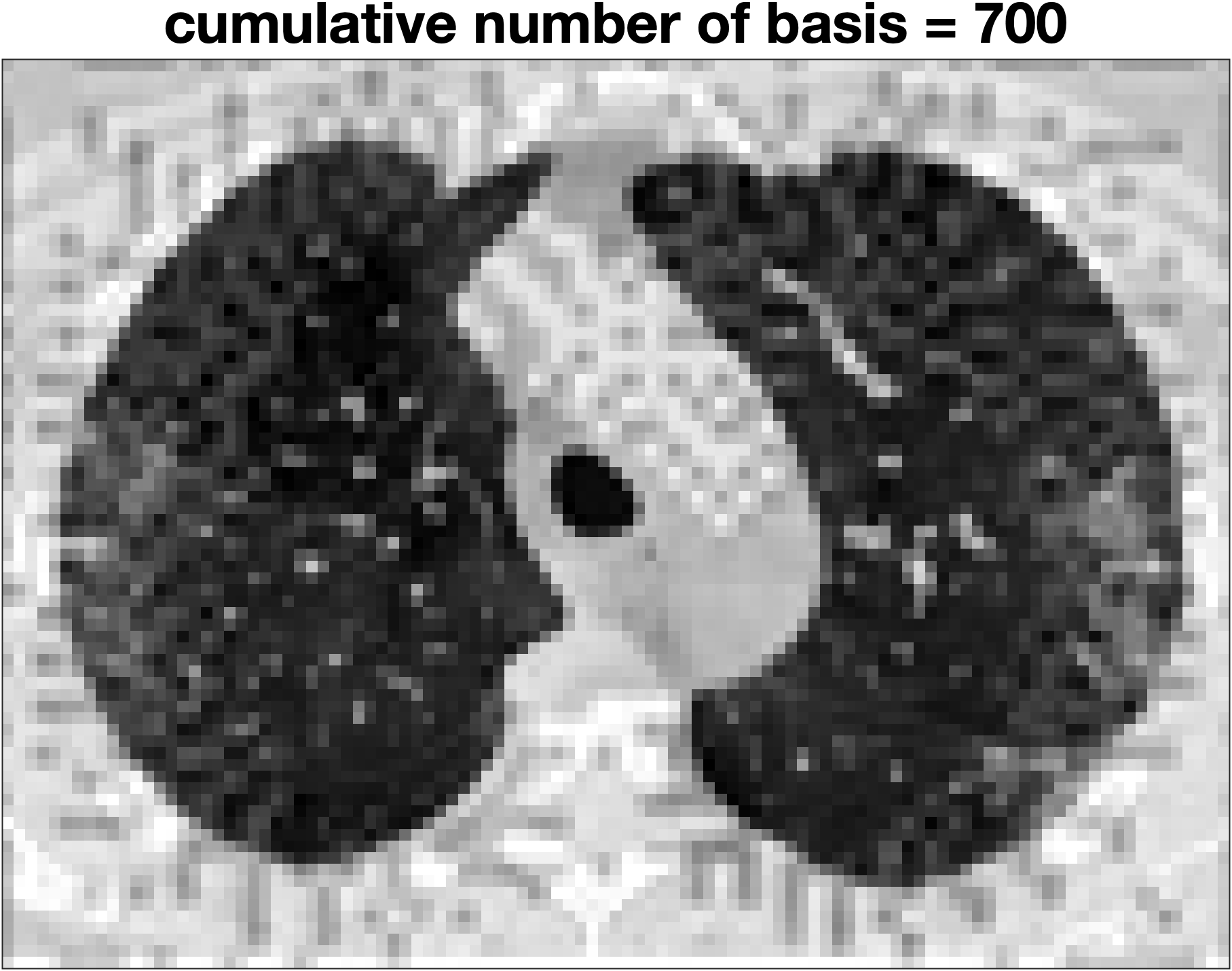
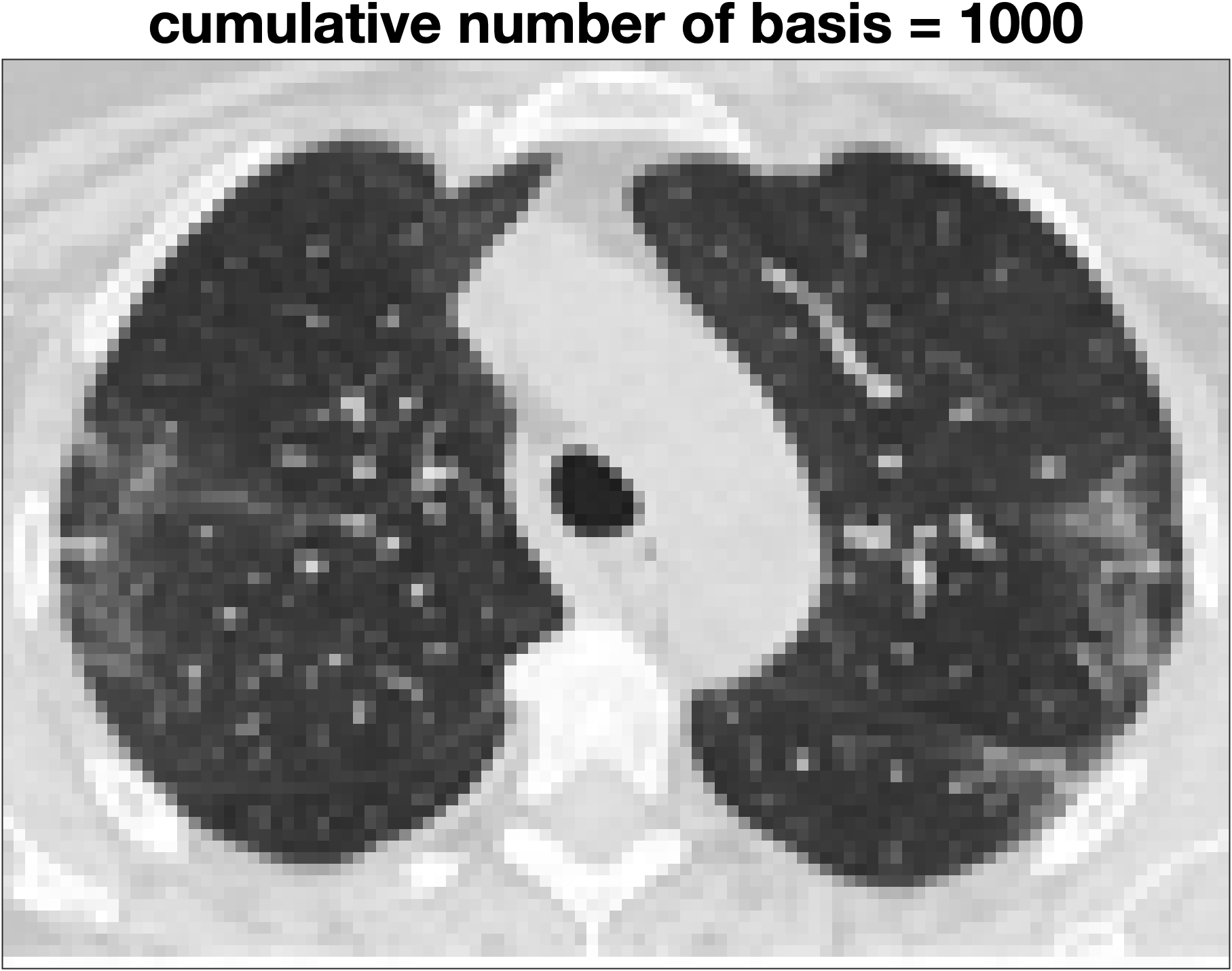
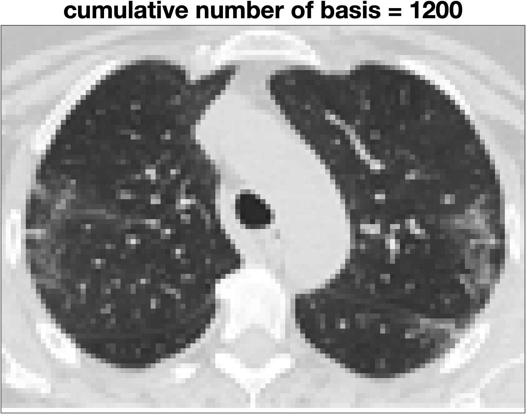
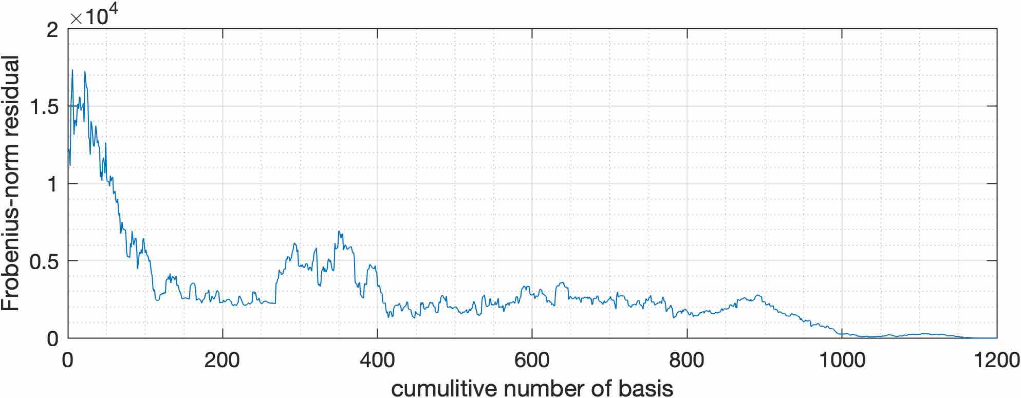
Figure F6: Reconstruction of an image using the patterns extracted in $V$. We can see the evolution of image as more patterns are added to it. The residual also drops relatively quickly. We have captured most distinctive features of the image by using about 400 patterns. Using 1,000 patterns captures the image almost perfectly.

The left basis defines how the patterns should be merged together. Images with lower norm in the left basis appear to have fewer distinctive features in them, as some of them are shown in Figure F7. In other word, they are made from fewer patterns in $V$. On the other hand, images with larger norm in the left basis have more distinctive features and many patterns contribute to them, as some of them are shown in Figure F8.

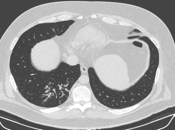
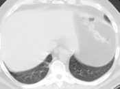
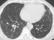
Figure F7: Images with small norm in the left basis appear are made from fewer patterns and appear to have less distinctive features.

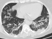
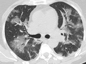
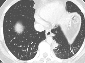
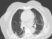
Figure F8: Images with large norm in the left basis appear relatively complex, have many distinctive features and many patterns contribute to them.

We note that evaluating the usefulness of our patterns, from the practical point of view, requires domain expertise. A radiology scientist, for example, could verify whether the patterns in Figure F4 are sensible and useful in practice.

Appendix G Demonstrating the effectiveness of wavelet transformation in our analysis

In all the results we have presented so far, we have relied on wavelet transformation of images. In this last appendix, we repeat some of our experiments without using the wavelet transformation, i.e., directly applying the Higher Order GSVD on the pixel information of images. In this experiment we use the COVID data in Appendix E.

For example, Figures G1 and G2 show the dominant patterns we obtain in $V$ for COVID and non-COVID patients. Compare these to the patterns we obtained in Figures F5 and F5, when we applied the HO-GSVD on the wavelet coefficients, instead of the pixels. Although the results obtained from the pixels seem to provide some information, they are relatively vague and scattered.

Figure G1: The most dominant patterns for COVID infected patients. This corresponds to Figure F4 which was obtained using wavelet transformation. The patterns obtained without the wavelets are relatively vague and scattered.

Figure G2: The most dominant patterns for non-COVID patients.

Moreover, Figure G3 shows the reconstruction of the same image as in Figure F6, this time with rank-1 patterns obtained without wavelet transformation.

Figure G3: Reconstruction of an image using the patterns extracted in $V$, by applying HO-GSVD directly on the pixel information of dataset. This is the same image as in Figure F6. This time, many of the patterns are adding noise to the image, leading to significant increase in the residual at the early stages of reconstruction.

Notice that in this reconstruction only 1,200 pixels (out of 8,190) are involved, as shown in Figure G4, and the rest of pixels are the same as the original image. Hence, the reconstruction without using the wavelets needs to start from an image mostly similar to the original image and cannot consider many of the pixels. This seems to hollow the point of performing low rank approximation.

Figure G4: 1,200 of the pixels with linearly independent variations among images. Some of these pixels are at the perimeter of image which clearly do not relate to COVID infection. Compare these pixels to the pixels in Figure F2, and how the 1,200 wavelet coefficients have engaged large and relevant regions of the image.

However, when using the 1,200 wavelet coefficients, the majority of pixels are involved in our analysis, as the stencil in Figure F2 demonstrates. Also, wavelets make the low rank approximations of images informative.

References

- Ali and Foroosh [2016] Muhammad Ali and Hassan Foroosh. Character recognition in natural scene images using rank-1 tensor decomposition. In IEEE International Conference on Image Processing, pages 2891–2895, 2016.
- Alter [2018] Orly Alter. Advanced tensor decompositions for computational assessment and prediction from data, October 18 2018. US Patent App. 15/566,298.
- Alter et al. [2000] Orly Alter, Patrick O Brown, and David Botstein. Singular value decomposition for genome-wide expression data processing and modeling. Proceedings of the National Academy of Sciences, 97(18):10101–10106, 2000.
- Alter et al. [2003] Orly Alter, Patrick O Brown, and David Botstein. Generalized singular value decomposition for comparative analysis of genome-scale expression data sets of two different organisms. Proceedings of the National Academy of Sciences, 100(6):3351–3356, 2003.
- Andrade-Loarca et al. [2019] Héctor Andrade-Loarca, Gitta Kutyniok, and Ozan Öktem. Shearlets as feature extractor for semantic edge detection: The model-based and data-driven realm. arXiv preprint arXiv:1911.12159, 2019.
- Angelov and Almeida Soares [2020] Plamen Angelov and Eduardo Almeida Soares. Explainable-by-design approach for COVID-19 classification via CT-scan. medRxiv, 2020.
- Arora et al. [2018] Sanjeev Arora, Rong Ge, Behnam Neyshabur, and Yi Zhang. Stronger generalization bounds for deep nets via a compression approach. In International Conference on Machine Learning, pages 254–263, 2018.
- Arora et al. [2019] Sanjeev Arora, Simon Du, Wei Hu, Zhiyuan Li, and Ruosong Wang. Fine-grained analysis of optimization and generalization for overparameterized two-layer neural networks. In International Conference on Machine Learning, pages 322–332, 2019.
- Bahri et al. [2020] Yasaman Bahri, Jonathan Kadmon, Jeffrey Pennington, Sam S Schoenholz, Jascha Sohl-Dickstein, and Surya Ganguli. Statistical mechanics of deep learning. Annual Review of Condensed Matter Physics, 2020.
- Belkin et al. [2006] Mikhail Belkin, Partha Niyogi, and Vikas Sindhwani. Manifold regularization: A geometric framework for learning from labeled and unlabeled examples. Journal of machine learning research, 7(Nov):2399–2434, 2006.
- Belkin et al. [2018] Mikhail Belkin, Siyuan Ma, and Soumik Mandal. To understand deep learning we need to understand kernel learning. In International Conference on Machine Learning, pages 541–549, 2018.
- Belkin et al. [2019] Mikhail Belkin, Alexander Rakhlin, and Alexandre B Tsybakov. Does data interpolation contradict statistical optimality? In The 22nd International Conference on Artificial Intelligence and Statistics, pages 1611–1619, 2019.
- Bertinetto et al. [2016] Luca Bertinetto, Jack Valmadre, Joao F Henriques, Andrea Vedaldi, and Philip HS Torr. Fully-convolutional siamese networks for object tracking. In European conference on computer vision, pages 850–865. Springer, 2016.
- Birodkar et al. [2019] Vighnesh Birodkar, Hossein Mobahi, and Samy Bengio. Semantic redundancies in image-classification datasets: The 10% you don’t need. arXiv preprint arXiv:1901.11409, 2019.
- Bradley et al. [2019] Matthew W Bradley, Katherine A Aiello, Sri Priya Ponnapalli, Heidi A Hanson, and Orly Alter. GSVD and tensor GSVD-uncovered patterns of DNA copy-number alterations predict adenocarcinomas survival in general and in response to platinum. APL Bioengineering, 3(3):036104, 2019.
- Bruna et al. [2016] Joan Bruna, Pablo Sprechmann, and Yann LeCun. Super-resolution with deep convolutional sufficient statistics. In International Conference on Learning Representations, 2016.
- Chan [1987] Tony F Chan. Rank revealing QR factorizations. Linear Algebra and its Applications, 88:67–82, 1987.
- Chen et al. [2016] Yushi Chen, Hanlu Jiang, Chunyang Li, Xiuping Jia, and Pedram Ghamisi. Deep feature extraction and classification of hyperspectral images based on convolutional neural networks. IEEE Transactions on Geoscience and Remote Sensing, 54(10):6232–6251, 2016.
- Daubechies [1990] Ingrid Daubechies. The wavelet transform, time-frequency localization and signal analysis. IEEE Transactions on Information Theory, 36(5):961–1005, 1990.
- Daubechies [1992] Ingrid Daubechies. Ten Lectures on Wavelets. Society for Industrial and Applied Mathematics, Philadelphia, 1992.
- De Lathauwer et al. [2000] Lieven De Lathauwer, Bart De Moor, and Joos Vandewalle. A multilinear singular value decomposition. SIAM journal on Matrix Analysis and Applications, 21(4):1253–1278, 2000.
- Effland et al. [2019] Alexander Effland, Erich Kobler, Thomas Pock, Marko Rajković, and Martin Rumpf. Image morphing in deep feature spaces: Theory and applications. arXiv preprint arXiv:1910.12672, 2019.
- Engstrom et al. [2020] Logan Engstrom, Andrew Ilyas, Shibani Santurkar, Dimitris Tsipras, Jacob Steinhardt, and Aleksander Madry. Identifying statistical bias in dataset replication. arXiv preprint arXiv:2005.09619, 2020.
- Fang et al. [2017] Leyuan Fang, Nanjun He, and Hui Lin. CP tensor-based compression of hyperspectral images. Journal of the Optical Society of America A, 34:252–258, 2017.
- Hand [2018] Emily M. Hand. Learning Explainable Facial Features from Noisy Unconstrained Visual Data. PhD thesis, University of Maryland, College Park, 2018.
- Hong et al. [2020] David Hong, Tamara G Kolda, and Jed A Duersch. Generalized canonical polyadic tensor decomposition. SIAM Review, 62(1):133–163, 2020.
- Huang and Anandkumar [2015] Furong Huang and Animashree Anandkumar. Convolutional dictionary learning through tensor factorization. In Feature Extraction: Modern Questions and Challenges, pages 116–129, 2015.
- Huang et al. [2019] Yujia Huang, Sihui Dai, Tan Nguyen, Richard G Baraniuk, and Anima Anandkumar. Out-of-distribution detection using neural rendering generative models. arXiv preprint arXiv:1907.04572, 2019.
- Ilyas et al. [2019] Andrew Ilyas, Shibani Santurkar, Dimitris Tsipras, Logan Engstrom, Brandon Tran, and Aleksander Madry. Adversarial examples are not bugs, they are features. In Advances in Neural Information Processing Systems, pages 125–136, 2019.
- Kolda and Bader [2009] Tamara G Kolda and Brett W Bader. Tensor decompositions and applications. SIAM Review, 51(3):455–500, 2009.
- Kolesnikov et al. [2019] Alexander Kolesnikov, Lucas Beyer, Xiaohua Zhai, Joan Puigcerver, Jessica Yung, Sylvain Gelly, and Neil Houlsby. Large scale learning of general visual representations for transfer. arXiv preprint arXiv:1912.11370, 2019.
- Krizhevsky [2009] Alex Krizhevsky. Learning multiple layers of features from tiny images. 2009.
- Kutyniok and Labate [2012] Gitta Kutyniok and Demetrio Labate. Shearlets: Multiscale analysis for multivariate data. Springer Science & Business Media, 2012.
- Labate et al. [2005] Demetrio Labate, Wang-Q Lim, Gitta Kutyniok, and Guido Weiss. Sparse multidimensional representation using shearlets. In Wavelets XI, volume 5914, page 59140U. International Society for Optics and Photonics, 2005.
- Lakshman et al. [2015] Haricharan Lakshman, W-Q Lim, Heiko Schwarz, Detlev Marpe, Gitta Kutyniok, and Thomas Wiegand. Image interpolation using shearlet based iterative refinement. Signal Processing: Image Communication, 36:83–94, 2015.
- LeCun et al. [1998] Yann LeCun, Léon Bottou, Yoshua Bengio, and Patrick Haffner. Gradient-based learning applied to document recognition. Proceedings of the IEEE, 86(11):2278–2324, 1998.
- Li et al. [2020] Jingling Li, Yanchao Sun, Jiahao Su, Taiji Suzuki, and Furong Huang. Understanding generalization in deep learning via tensor methods. arXiv preprint arXiv:2001.05070, 2020.
- Liang et al. [2018] Shiyu Liang, Yixuan Li, and Rayadurgam Srikant. Enhancing the reliability of out-of-distribution image detection in neural networks. In International Conference on Learning Representations, 2018.
- Maaten and Hinton [2008] Laurens van der Maaten and Geoffrey Hinton. Visualizing data using t-SNE. Journal of Machine Learning Research, 9:2579–2605, 2008.
- Neyshabur et al. [2019] Behnam Neyshabur, Zhiyuan Li, Srinadh Bhojanapalli, Yann LeCun, and Nathan Srebro. Towards understanding the role of over-parametrization in generalization of neural networks. In International Conference on Learning Representations, 2019.
- Noh et al. [2017] Hyeonwoo Noh, Andre Araujo, Jack Sim, Tobias Weyand, and Bohyung Han. Large-scale image retrieval with attentive deep local features. In Proceedings of the IEEE International Conference on Computer Vision, pages 3456–3465, 2017.
- Omberg et al. [2007] Larsson Omberg, Gene H Golub, and Orly Alter. A tensor higher-order singular value decomposition for integrative analysis of DNA microarray data from different studies. Proceedings of the National Academy of Sciences, 104(47):18371–18376, 2007.
- Parde et al. [2017] Connor J Parde, Carlos Castillo, Matthew Q Hill, Y Ivette Colon, Swami Sankaranarayanan, Jun-Cheng Chen, and Alice J O’Toole. Face and image representation in deep CNN features. In 12th IEEE International Conference on Automatic Face & Gesture Recognition, pages 673–680, 2017.
- Perros et al. [2019] Ioakeim Perros, Evangelos E Papalexakis, Richard Vuduc, Elizabeth Searles, and Jimeng Sun. Temporal phenotyping of medically complex children via PARAFAC2 tensor factorization. Journal of Biomedical Informatics, 93:103125, 2019.
- Ponnapalli et al. [2011] Sri Priya Ponnapalli, Michael A Saunders, Charles F Van Loan, and Orly Alter. A higher-order generalized singular value decomposition for comparison of global mRNA expression from multiple organisms. PloS One, 6(12), 2011.
- Recht et al. [2018] Benjamin Recht, Rebecca Roelofs, Ludwig Schmidt, and Vaishaal Shankar. Do CIFAR-10 classifiers generalize to CIFAR-10? arXiv preprint arXiv:1806.00451, 2018.
- Recht et al. [2019] Benjamin Recht, Rebecca Roelofs, Ludwig Schmidt, and Vaishaal Shankar. Do ImageNet classifiers generalize to ImageNet? In International Conference on Machine Learning, pages 5389–5400, 2019.
- Ren et al. [2019] Jie Ren, Peter J Liu, Emily Fertig, Jasper Snoek, Ryan Poplin, Mark Depristo, Joshua Dillon, and Balaji Lakshminarayanan. Likelihood ratios for out-of-distribution detection. In Advances in Neural Information Processing Systems, pages 14680–14691, 2019.
- Romero et al. [2015] Adriana Romero, Carlo Gatta, and Gustau Camps-Valls. Unsupervised deep feature extraction for remote sensing image classification. IEEE Transactions on Geoscience and Remote Sensing, 54(3):1349–1362, 2015.
- Savas and Eldén [2007] Berkant Savas and Lars Eldén. Handwritten digit classification using higher order singular value decomposition. Pattern Recognition, 40(3):993–1003, 2007.
- Schug et al. [2015] David A Schug, Glenn R Easley, and Dianne P O’Leary. Wavelet–shearlet edge detection and thresholding methods in 3d. In Excursions in Harmonic Analysis, Volume 3, pages 87–104. Springer, 2015.
- Sedghi et al. [2019] Hanie Sedghi, Vineet Gupta, and Philip M. Long. The singular values of convolutional layers. In International Conference on Learning Representations, 2019.
- Shafahi et al. [2019] Ali Shafahi, W Ronny Huang, Christoph Studer, Soheil Feizi, and Tom Goldstein. Are adversarial examples inevitable? In International Conference on Learning Representations, 2019.
- Strang [2019] Gilbert Strang. Linear Algebra and Learning from Data. Wellesley-Cambridge Press, 2019.
- Thom and Hand [2020] Nathan Thom and Emily M. Hand. Facial Attribute Recognition: A Survey, pages 1–13. Springer International Publishing, 2020.
- Tsipras et al. [2019] Dimitris Tsipras, Shibani Santurkar, Logan Engstrom, Alexander Turner, and Aleksander Madry. Robustness may be at odds with accuracy. In International Conference on Learning Representations, 2019.
- Van Loan [1976] Charles F Van Loan. Generalizing the singular value decomposition. SIAM Journal on Numerical Analysis, 13(1):76–83, 1976.
- Vo et al. [2019] Huy V Vo, Francis Bach, Minsu Cho, Kai Han, Yann LeCun, Patrick Pérez, and Jean Ponce. Unsupervised image matching and object discovery as optimization. In Proceedings of the IEEE Conference on Computer Vision and Pattern Recognition, pages 8287–8296, 2019.
- Yadav and Bottou [2019] Chhavi Yadav and Léon Bottou. Cold case: The lost MNIST digits. In Advances in Neural Information Processing Systems, pages 13443–13452, 2019.
- Yousefzadeh [2020] Roozbeh Yousefzadeh. Using wavelets to analyze similarities in image-classification datasets. arXiv preprint arXiv:2002.10257, 2020.
- Yousefzadeh and O’Leary [2020] Roozbeh Yousefzadeh and Dianne P O’Leary. Deep learning interpretation: Flip points and homotopy methods. In Mathematical and Scientific Machine Learning Conference, 2020.
- Zhang et al. [2017] Chiyuan Zhang, Samy Bengio, Moritz Hardt, Benjamin Recht, and Oriol Vinyals. Understanding deep learning requires rethinking generalization. In International Conference on Learning Representations, 2017.