Optical studies of two stripped envelope supernovae $-$ SN 2015ap (Type Ib) and SN 2016P (Type Ic)

Abstract

We present the photometric and spectroscopic studies of a Type Ib SN 2015ap and a Type Ic SN 2016P. SN 2015ap is one of the bright (M_V = $-$18.04 mag) Type Ib while SN 2016P lies at an average value among the Type Ic SNe (M_V = $-$17.53 mag). Bolometric light curve modelling of SNe 2015ap and 2016P indicates that both the SNe are powered by ⁵⁶Ni + magnetar model with ⁵⁶Ni masses of 0.01 M_⊙ and 0.002 M_⊙, ejecta masses of 3.75 M_⊙ and 4.66 M_⊙, spin period P₀ of 25.8 ms and 36.5 ms and magnetic field B_p of 28.39 $\times$ 10¹⁴ Gauss and 35.3 $\times$ 10¹⁴ Gauss respectively. The early spectra of SN 2015ap shows prominent lines of He with a “W" feature due to Fe complexes while other lines of Mg II, Na I and Si II are present in both SNe 2015ap and 2016P. Nebular phase [O I] profile indicates an asymmetric profile in SN 2015ap. The [O I]/[Ca II] ratio and nebular spectral modelling of SN 2015ap hints towards a progenitor mass between 12 $-$ 20 M_⊙.

1 Introduction

Massive stars undergoing catastrophic explosions at the end of their life are coined as core-collapse supernovae (CCSNe; Woosley & Weaver, 1986; Heger et al., 2003; Smartt, 2009). Among the group of CCSNe, lies the stripped envelope (SE-SNe) members called SNe of Type IIb, Ib and Ic which strip off their outer Hydrogen or Helium layer before the explosion (Clocchiatti & Wheeler, 1997). Stripping occurs either due to radiation driven stellar winds (Puls et al., 2008), heavy mass-loss (Smith & Owocki, 2006), or mass-transfer with a companion star (Wheeler & Levreault, 1985; Podsiadlowski et al., 1992; Yoon et al., 2010). Classically, Type Ib SNe show He features and Type Ic are devoid of He features (Filippenko, 1997). However, studies by Woosley et al. (1995); Dessart et al. (2012); Cano et al. (2014) suggest that in Type Ic, either Helium is hidden because of improper excitation due to poor mixing or is completely absent. A small fraction of Type Ic SNe ($\sim$ 4 $\%$; Shivvers et al., 2017) show broad absorption lines in their spectra around maximum light with expansion velocities between 15,000 km s^-1 to 30,000 km s^-1. These are known as broad-lined Type Ic SNe (BL-Ic). Some of the BL-Ic SNe are linked with gamma ray bursts (GRBs) and X-ray flashes (XRFs) (for example SN 1998bw/GRB 980425; Galama et al. (1999), SN 2006aj/XRF 060218; Modjaz et al. (2006)).

A number of studies have been made by several authors to investigate the photometric (Richardson et al., 2006; Drout et al., 2011; Cano, 2013; Bianco et al., 2014; Pritchard et al., 2014; Taddia et al., 2015; Lyman et al., 2016; Prentice et al., 2016) and spectroscopic properties of SE-SNe (Matheson, 2001; Modjaz et al., 2016; Prentice et al., 2019). These studies have shown a wide diversity in terms of both light curve shapes and spectral features in SE-SNe. The typical rise time of SE-SNe is found to be 10$-$20 days (Prentice et al., 2019) with weighted peak absolute magnitude of M_V = $-$18.03 $\pm$ 0.06 mag (Richardson et al., 2006). Lyman et al. (2016) found a considerable spread of $\sim$ 3 mag in the absolute magnitude light curves of SE-SNe. Taddia et al. (2018) found a correlation between late-time slopes and $\triangle m_{15}$, which is the decay rate from peak upto 15 days post maximum, suggesting that light curves with initial steeper slopes decline faster at later stages.

The ⁵⁶Ni mass, ejecta mass and kinetic energy can be measured by modelling the bolometric light curves. Cano (2013) estimated median ⁵⁶Ni mass between 0.15$-$0.18 M_⊙ and ejecta masses of 3.9 M_⊙ and 3.4 M_⊙ for Type Ib and Type Ic SNe respectively. While Taddia et al. (2018) found ejecta masses for SE-SNe to be between 1.1 – 6.2 M_⊙, Prentice et al. (2019) quote the median distribution to be 2.8 $\pm$ 1.5 M_⊙. Even though high ejecta masses for Type Ic SNe indicates higher progenitor masses, the distribution of ejecta masses for Type Ic SNe hints towards a wide distribution of progenitor masses. Also, the ejecta mass distribution for both Type Ib and Ic SNe are inconsistent with massive single stars and support moderate mass stars in binary associations (Lyman et al., 2016). The most common technique used for direct detection of progenitors involve analysing the pre-explosion images. So far direct detection has been possible for only one Type Ib SN iPTF13bvn (Cao et al., 2013; Groh et al., 2013; Bersten et al., 2014; Fremling et al., 2014; Kuncarayakti et al., 2015; Folatelli et al., 2016; Fremling et al., 2016; Eldridge & Maund, 2016; Hirai, 2017a, b) and one Type Ic SN 2017ein (Van Dyk et al., 2018; Kilpatrick et al., 2018). The progenitor masses of iPTF13bvn and SN 2017ein were found to be 10$-$20 M_⊙ (Cao et al., 2013; Groh et al., 2013) and 47$-$80 M_⊙ (Van Dyk et al., 2018; Kilpatrick et al., 2018) respectively although the progenitor detection of SN 2017ein is debated (Van Dyk et al., 2018; Kilpatrick et al., 2018).

Metallicity and rotation largely affects the predicted ratios of Type Ib/c SNe, mass-loss rates and the production of WR stars (Eldridge et al., 2008). Eldridge et al. (2008) have shown that stars with high ejecta mass come from massive progenitors. However, if fallback occurs, even less massive stars can eject more mass (for example SN 1999dn, Benetti et al., 2011). Kuncarayakti et al. (2015) favour low mass binary systems as progenitors of Type Ib/c SNe. On the other hand, Galbany et al. (2018) claimed that Type Ic SNe have the most massive progenitors. But, both Kuncarayakti et al. (2015) and Galbany et al. (2018) suggest the origin of Type Ib/c SNe from young stellar populations. Thus, the exact characterisation of ejecta mass, energy and consecutively the progenitor system remains largely uncertain.

In this paper, we present the photometric and spectroscopic study of a Type Ib SN 2015ap and a Type Ic SN 2016P. The SNe details are given in section 2. The data acquisition and reduction procedures are described in section 3. Temporal evolution of the multi-band light curves and colour curves are studied in section 4 along with the analytical modelling of the bolometric light curve. A detailed description of the spectral evolution and asymmetry in the nebular phase are presented in sections 5 and 6 respectively. Section 7 summarises the main results of this study.

2 Parameters of SNe

2.1 SN 2015ap

SN 2015ap was discovered by Lick Observatory Supernova Search (LOSS) on 2015, September 08 by Ross, Zheng, Filippenko at R.A.= 02^h05^m13.3^s, Decl.= +06^∘06${}^{{}^{\prime}}$08${}^{{}^{\prime\prime}}$ (J2000.0). The SN was located 28".7 west and 16".4 south of the center of the host galaxy IC 1776 at a redshift of 0.01138. The classification spectrum was obtained with Copernico 1.82 m telescope (+AFOSC; range 340-820 nm; resolution 1.4 nm) operated by INAF Astronomical observatory of Padova in Asiago, Mount Ekar, Italy, on 2015, September 11 (Tartaglia et al., 2015) and the spectrum was found to be similar to those of several broad-lined Type Ib/c SNe close to maximum light. It was re-classified as Type Ib SN using the spectrum obtained on 2015 September 21 by 201 . We used the GEneric cLAssification TOol (GELATO) (Harutyunyan et al., 2008) on the first three spectra of SN 2015ap. GELATO compares bins of the spectrum to those of template SNe at similar epochs which suggests that the explosion occurred on 2015 September 05 $\pm$ 1. However, GELATO results will be reasonable only if the light curves also match. We match the $V$-band light curve of SN 2015ap with the light curves of the SNe in our comparison sample (see section 4). Performing a template fitting method by applying a simultaneous shift in phase and magnitude, we find that the light curve of SN 2007gr best matches our observed light curve which constrains the explosion epoch as 2015 September 07 $\pm$ 1. To further constrain the explosion epoch, we performed a parabolic fit (described in Gangopadhyay et al. (2018)) to the $V$-band light curve and infer the explosion epoch to be 2015 September 07. Based on the above methods, we conclude that the explosion occurred between 2015 September 04 to 08. We adopt a distance modulus of $\mu$ = 33.27 $\pm$ 0.15 mag for the host galaxy IC 1776 and total A_V = 0.115 mag along the line of sight (negligible host extinction) from Prentice et al. (2019).

2.2 SN 2016P

SN 2016P was discovered on 2016 January 19, 21".7 east and 2".8 north of the center of the host galaxy NGC 5374 at R.A. = 13^h57^m31.13^s, Dec = +06^∘05${}^{{}^{\prime}}$51.6${}^{{}^{\prime\prime}}$ (J2000.0). An optical spectrum obtained with YFOSC at Yunnan Astronomical Observatories on 2015 January 19.9 was found to be consistent with a BL Ic SN a few days before maximum light (Zhang & Wang, 2016). Following the same approach as in SN 2015ap, GELATO runs on the first three spectra of SN 2016P estimates the explosion epoch to be 2016 January 15 $\pm$ 1. The light curve template fitting method gives a best match with SN 2007ru and constrains the explosion epoch to be 2016 January 18 $\pm$ 3. The parabolic fit to the $V$-band light curve upto 10 days estimates the explosion epoch to be around 2016 January 15 $\pm$ 1. The bolometric light curve modelling (see section 4.2) gives the explosion epoch to be 2016 January 15. The results of the above methods constrains the explosion epoch to be between 2016 January 14 $-$ 18 (since discovery was on 2016 January 19, we constrain it upto 2016 January 18). From Prentice et al. (2019), we adopt a distance modulus of $\mu$ = 34.19 $\pm$ 0.15 mag for the host galaxy NGC 5374. The galactic E(B-V) along the line of sight of SN 2016P is 0.024 mag (Schlafly & Finkbeiner, 2011). Using the equivalent width of the NaID line Prentice et al. (2019) estimate the host galaxy E(B-V) = 0.05 $\pm$ 0.02 mag. Due to the poor resolution in our observed spectra, we were unable to measure the equivalent width of the NaID line. We adopt a total extinction of A_V = 0.229 $\pm$ 0.092 mag along the line of sight of SN 2016P from Prentice et al. (2019).

3 Data Acquisition and Reduction

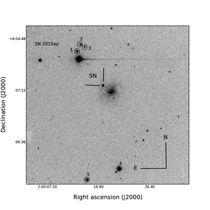
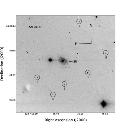
Figure 21: SNe 2015ap and 2016P and the local standard stars in the field of IC 1776 and NGC 5374, $R$-band, 300 sec image obtained on 2015 September 26 and 2016 January 23 with the 2.0m HCT for SNe 2015ap and 2016P respectively.

Photometric observing campaigns were carried out from 2015 September 18 to 2016 August 27 for SN 2015ap and from 2016 January 21 to 2016 June 03 for SN 2016P respectively using 1.04m Sampurnanand Telescope (ST); 1.30m Devasthal Fast Optical Telescope (DFOT) located in ARIES, Nainital, India; Copernico 1.82m Telescope operated by INAF Astronomical University of Padova (Mount Ekar), Italy; 2.00m Himalayan Chandra Telescope (HCT), IAO, Hanle, India and 2.54m Nordic Optical Telescope (NOT), La Palma, Canary Island. The imaging observations were done using Johnson-Cousin-Bessel UBVRI and SDSS ugriz filters. Image reduction and photometry were done using IRAF and DAOPHOT following the same steps as outlined in Gangopadhyay et al. (2018) and briefly described in Appendix A. The SN magnitudes were calibrated with respect to the local standards (Fig 21,Tables 5 and 6). The final magnitudes of SNe 2015ap and 2016P are given in Table 7 and Table 8 respectively.

Low and medium resolution optical spectra of SN 2015ap were obtained with 2.0m HCT and Copernico 1.82m telescope at 14 epochs. For SN 2016P, spectra were obtained at six epochs with HCT. The spectroscopic reduction was done using standard packages in IRAF. The spectra were wavelength and flux calibrated following the steps described in Gangopadhyay et al. (2018). The log of spectroscopic observations is presented in Table 9 and Table 10.

4 Temporal evolution of SNe 2015ap and 2016P

Table 1: Parameters of SNe 2015ap and 2016P

SN 2015ap	$B$ band	$V$ band	$R$ band	$I$ band
MJD (maximum)	57283.0 $\pm$ 0.5	57284.9 $\pm$ 0.5	57289.3 $\pm$ 0.5	57287.5 $\pm$ 0.5
Magnitude at maximum (mag)	15.54 $\pm$ 0.03	15.23 $\pm$ 0.02	15.16 $\pm$ 0.02	14.76 $\pm$ 0.04
Absolute magnitude at maximum (mag)	-17.71 $\pm$ 0.19	-18.04 $\pm$ 0.19	-18.15 $\pm$ 0.17	-18.54 $\pm$ 0.16
$\Delta$m15 (mag)	1.73 $\pm$ 0.10	1.03 $\pm$ 0.07	0.74 $\pm$ 0.05	0.58 $\pm$ 0.05
Rise time (rest-frame-day)	9.9	11.8	16.1	14.3
SN 2016P	$B$ band	$V$ band	$R$ band	$I$ band
MJD (maximum)	57413.03 $\pm$ 0.5	57416.75 $\pm$ 0.5	57417.20 $\pm$ 0.5	57418.36 $\pm$ 0.5
Magnitude at maximum (mag)	17.37 $\pm$ 0.05	16.64 $\pm$ 0.08	16.36 $\pm$ 0.08	16.15 $\pm$ 0.05
Absolute magnitude at maximum (mag)	-16.89 $\pm$ 0.12	-17.53 $\pm$ 0.14	-17.81 $\pm$ 0.13	-17.92 $\pm$ 0.11
$\Delta$m15 (mag)	1.47 $\pm$ 0.12	1.20 $\pm$ 0.06	0.93 $\pm$ 0.04	0.63 $\pm$ 0.05
Rise time (rest-frame-day)	6.9	10.6	11.0	12.4

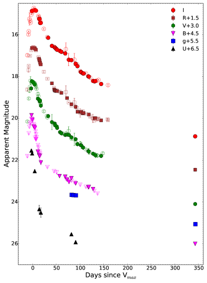
Figure 1: UgBVRI light curve evolution of SN 2015ap. The filled symbols represent our data and open symbols represent the data taken from Prentice et al. 2019.

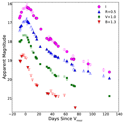
Figure 2: BVRI light curve evolution of SN 2016P. The filled symbols represent our data and open symbols represent the data taken from Prentice et al. 2019.

The complete multi-band optical light curve of SNe 2015ap and 2016P are shown in Fig 1 and Fig 2 respectively. The date of maximum and brightness at peak in different bands were determined by fitting a cubic spline to the BVRI light curve of both the SNe and are listed in Table 1. The maximum in $V$-band for SNe 2015ap and 2016P occurred on MJD 57284.86 $\pm$ 0.50 and 57416.75 $\pm$ 0.50 at an apparent magnitude of 15.23 $\pm$ 0.02 mag and 16.64 $\pm$ 0.08 mag respectively. The errors reported are obtained from the interpolated measurements around the peak. We notice that there is a gradual delay in reaching the maximum in the redder passbands. We use days since $V$-maximum as a reference epoch throughout the paper.

The light curve features of SNe 2015ap and 2016P are compared with those of other well-studied SNe Ib/c in Fig 3. We construct a sample of SNe Ib/c from literature and list their parameters in Table 2. The comparison sample chosen is vast and diverse. While SNe 2009jf and iPTF13bvn are fast evolving, SNe 1999dn is a prototypical Type Ib SN. Type Ic sample consists of both normal and BL-Ic’s to highlight the diversity in this sub-class. We have also included both fast and slow-evolving Type Ic which enables us to make a direct comparison with SN 2016P. In addition to these, we have also selected those Type Ib/c SNe from Prentice et al. (2019) which have observations in the B and the V-bands that are consistent with our observations. This comparison sample represents the properties of the Type Ib/c population.

Fig 3 shows the light curve evolution up to 150 days post $V$-maximum. The observed SN magnitudes of SNe 2015ap and 2016P along with the comparison sample are normalised with respect to their respective peak magnitudes, and a shift in the time is applied to match the time of maximum. To compare the light curve evolution of Type Ib/c SNe, we estimated decline of the light-curve in the first 15 days after peak ($\triangle m_{15}$) and late phase decline rate between 50$-$100 days. The decline rates are listed in Table 3.

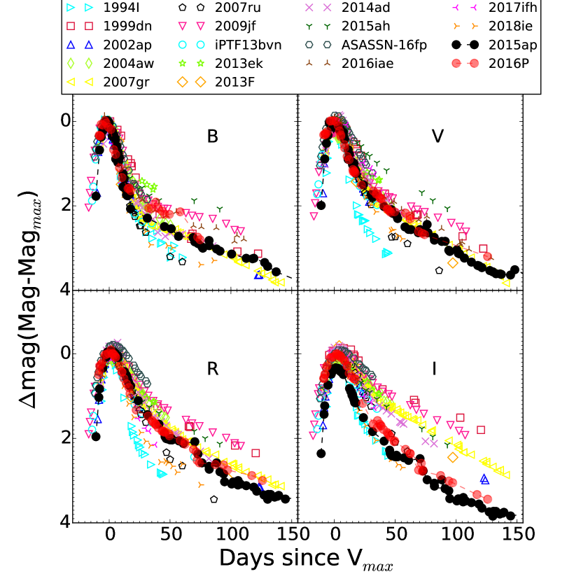
Figure 3: BVRI/ri light curve evolution of SN 2015ap and SN 2016P compared with other members of the sub-class. All the light curves are shifted in phase and matched to maximum light.

Table 2: Properties of the comparison sample

SNe	Host galaxy	Distance	Extinction	SN Type	Peak Absmag‡	MNi	Mej	Ek	Reference†
		(Mpc)	E(B-V)		$V$-band	M⊙	M⊙	1052 erg
SN 1999dn	NGC 7714	38.5	0.100	Ib	-16.88	0.09 $\pm$ 0.04	5.13 $\pm$ 1.82	0.37 $\pm$ 0.13	2,11,12
SN 2009jf	NGC 7479	33.7	0.110	Ib	-17.90	0.18 $\pm$ 0.04	7.34 $\pm$ 1.0	1.05 $\pm$ 0.15	4,11
iPTF 13bvn	NGC 5806	23.9	0.215	Ib	-17.35	0.09	1.5 $-$ 2.2	0.1	5
SN 2013ek	NGC 6984	50.1	0.037	Ib	-17.22	0.05 $\pm$ 0.01	1.2	0.04	13
SN 2015ah	UGC12295	58.9	0.091	Ib	-17.53	0.092 $\pm$ 0.07	2	0.09	13
SN 1994I	M51	6.3	0.452	Ic	-17.49	0.06 $\pm$ 0.01	0.72 $\pm$ 0.04	0.07 $\pm$ 0.01	1,11,12
SN 2002ap	NGC 0628	9.9	0.090	Ic-BL	-18.11	0.09	$\geq$ 1.5	—	6
SN 2004aw	NGC 3997	72.8	0.092	Ic	-17.30	0.22 $\pm$ 0.08	6.49 $\pm$ 2.32	0.90 $\pm$ 0.32	7,11,12
SN 2007gr	NGC 1058	9.7	0.092	Ic	-17.11	0.04 $\pm$ 0.01	1.70 $\pm$ 0.23	0.08 $\pm$ 0.01	3,11,12
SN 2007ru	UGC 12381	64.2	0.270	Ic-BL	-18.92	0.34 $\pm$ 0.09	3.59 $\pm$ 1.52	1.43 $\pm$ 0.57	8,11,12
SN 2013F	IC 5325	17.6	1.418	Ic	-18.55	0.15	1.4	0.11	13
SN 2014ad	MRK 1309	26.6	0.220	Ic-BL	-18.72	0.24	3.3 $\pm$ 0.8	1 $\pm$ 0.3	9,12
ASASSN-16fp	NGC 5806	23.9	0.074	Ic	-18.36	0.1	4.5 $\pm$ 0.3	0.69	10,12
SN 2016iae	NGC 1532	17.3	0.664	Ic	-18.23	0.13	2.2	0.18	13
SN 2017ifh	2MASX J06350438+5026278	156.3	0.167	Ic-BL	-18.55	0.16 $\pm$ 0.01	3.0	0.77	13
SN 2018ie	NGC 3456	46.8	0.08	Ic-BL	-16.94	0.026 $\pm$ 0.002	1.5	0.79	13

^† REFERENCES.– (1)Richmond et al. (1996); (2)Benetti et al. (2011); (3)Hunter et al. (2009); (4)Sahu et al. (2011), NED; (5)Srivastav et al. (2014), NED; (6)Yoshii et al. (2003); Foley et al. (2003), NED; (7)Taubenberger et al. (2006), NED; (8)Sahu et al. (2009); (9)Sahu et al. (2018); (10)Kumar et al. (2018); (11)Cano (2013); (12) NED; (13)Prentice et al. (2019). ^‡ Values are scaled with respect to H_o = 73 km sec^-1 Mpc^-1.

Drout et al. (2011) states that the average value of $\triangle m_{15}(V)$ and $\triangle m_{15}(R)$ from a literature sample of Type Ib/c SNe are 0.94 $\pm$ 0.31 mag and 0.74 $\pm$ 0.21 mag respectively. For an individual Type Ib, Ic and Ic-BL sample, Drout et al. (2011) estimate $\triangle m_{15}(R)$ to be 0.7 $\pm$ 0.1 mag, 0.9 $\pm$ 0.5 mag and 0.7 $\pm$ 0.1 mag. The $\triangle m_{15}(V)$ values of SN 2015ap matches well with iPTF13bvn, is higher than the value quoted in Drout et al. (2011) but is consistent with the values reported in Taddia et al. (2018). The $\triangle m_{15}$ values in SN 2016P are in between those of the Type Ic comparison sample used in this work, however they are a bit faster than the average values reported in Drout et al. (2011) and Taddia et al. (2018). The late-time light curves are faster than the average decay rate of ⁵⁶Co to ⁵⁶Fe. Taddia et al. (2018) estimated the late time decay rates between 1.4 – 1.8 mag (100 days)^-1 and 1.7 – 2.7 mag (100 days)^-1 for Type Ib and Type Ic sample respectively. Table 3 and Fig 3, thus, shows that both SNe 2015ap and 2016P shows faster evolution than the ⁵⁶Co – ⁵⁶Fe decay rates. This implies inefficient $\gamma$-ray trapping for both the SNe.

Table 3: Early and late time decay rates of a sample of Type Ib/c SNe.

Supernova	$\triangle m_{15}$ (mag)		Late time (50-100 days) decay rates (mag (100 days)-1)				Reference
	$V$	$R$	$B$	$V$	$R$	$I$
SN 1999dn	0.49 $\pm$ 0.08	0.31 $\pm$ 0.03	1.07 $\pm$ 0.19	1.54 $\pm$ 0.09	1.32 $\pm$ 0.09	1.15 $\pm$ 0.07	3
SN 2007gr	1.31 $\pm$ 0.05	0.46 $\pm$ 0.07	1.11 $\pm$ 0.06	1.70 $\pm$ 0.05	1.94 $\pm$ 0.07	1.64 $\pm$ 0.04	3,1
SN 2009jf	0.50	0.31	0.89 $\pm$ 0.14	1.36 $\pm$ 0.07	1.61 $\pm$ 0.02	1.71 $\pm$ 0.11	4,5
iPTF13bvn	1.01	0.90	—	—	—	—	10
SN 2013ek	0.78 $\pm$ 0.08	0.60 $\pm$ 0.10	—	—	—	—	12,3
SN 2015ah	0.83 $\pm$ 0.04	0.71 $\pm$ 0.01	—	—	—	—	12,3
SN 2015ap	1.03 $\pm$ 0.07	0.74 $\pm$ 0.05	1.10 $\pm$ 0.15	1.55 $\pm$ 0.14	2.14 $\pm$ 0.18	1.88 $\pm$ 0.17	3
SN 1994I	1.74 $\pm$ 0.02	1.46 $\pm$ 0.02	—	1.84 $\pm$ 0.05	—	—	2
SN 2002ap	1.85 $\pm$ 0.45	—	1.70 $\pm$ 0.04	2.10 $\pm$ 0.02	1.60 $\pm$ 0.01	1.70 $\pm$ 0.01	3,6
SN 2004aw	0.62 $\pm$ 0.03	0.41 $\pm$ 0.03	1.35 $\pm$ 0.18	1.74 $\pm$ 0.22	1.36 $\pm$ 0.14	1.53 $\pm$ 0.19	5
SN 2007ru	0.92	0.69	—	2.1	2.8	3.0	7
SN 2013F	1.43 $\pm$ 0.26	1.05 $\pm$ 0.28	—	—	—	—	12,3
SN 2014ad	0.95 $\pm$ 0.06	0.77 $\pm$ 0.03	0.89 $\pm$ 0.10	2.19 $\pm$ 0.13	2.17 $\pm$ 0.05	2.04 $\pm$ 0.11	3,8
ASASSN-16fp	0.60 $\pm$ 0.02	0.42 $\pm$ 0.02	—	—	—	—	3,9
SN 2016iae	0.91 $\pm$ 0.25	—	1.29 $\pm$ 0.24	1.61 $\pm$ 0.19	—	—	12,3
SN 2018ie	1.41 $\pm$ 0.16	1.06 $\pm$ 0.13	—	—	—	—	12,3
SN 2016P	1.20 $\pm$ 0.06	0.93 $\pm$ 0.04	—	1.75 $\pm$ 0.22	1.78 $\pm$ 0.18	2.09 $\pm$ 0.21	3
Type Ib/c, Ic-BL	0.94 $\pm$ 0.31	0.74 $\pm$ 0.21	—	—	—	—	11
Type Ib SNe	1.03 $\pm$ 0.19	0.75 $\pm$ 0.21	—	—	—	—	13
Type Ic SNe	0.90 $\pm$ 0.22	0.62 $\pm$ 0.24	—	—	—	—	13

^† REFERENCES.–(1) Hunter et al. (2009); (2) Richmond et al. (1996); (3) This work ; (4) Taubenberger et al. (2006);
(5) Valenti et al. (2011); Sahu et al. (2011); (6) Hunter et al. (2009); (7) Sahu et al. (2009); (8) Sahu et al. (2018);
(9) Kumar et al. (2018); (10) Srivastav et al. (2014); (11) Drout et al. (2011); (12) Prentice et al. (2019); (13) Taddia et al. (2018)

4.1 Colour evolution of SNe 2015ap and 2016P

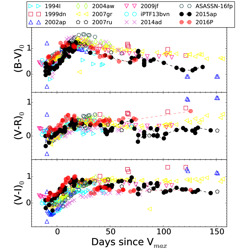
Figure 4: A comparison of the (B-V)₀, (V-R)₀ and (V-I)₀ colours of SNe 2015ap and 2016P with other representative SNe Ib/c. The colours are corrected for the reddening values given in Table 2.

The colour evolution of SNe 2015ap and 2016P along with other members of the comparison sample are displayed in Fig 4. A diversity exists among the colour variation due to expansion of photospheric envelope and the changing temperatures. All the colour curves have been dereddened by the value reported in Table 2. The pre-maximum $(B-V)_{o}$ colours of all the SNe are similar and bluer which occurs due to the increase in photospheric temperatures as SN brightens. From $-$11 day to 2 day, the $(B-V)_{o}$ colours of SN 2015ap increases from 0.12 mag to 0.61 mag. During the maximum light, the $(B-V)_{o}$ colour remains around 1.1 mag and becomes bluer post 100 day. The $(B-V)_{o}$ colour evolution of SN 2015ap is similar to all the SNe of Type Ib comparison sample. A similar trend is noticed for the $(V-R)_{o}$ colours of SN 2015ap which is blue ($\sim$ 0.03 mag) at pre-maximum and becomes redder with time. Drout et al. (2011) found that the average $(V-R)_{o}$ colour 10 days post $V$-maximum should be around 0.26 $\pm$ 0.10 mag for Type Ib/c SNe, if the estimated extinction are well within errors. The $(V-R)_{o}$ colour of SN 2015ap is between 0.25 mag to 0.35 mag around 10 days post $V$-maximum which is well in agreement with the values of Drout et al. (2011). A similar trend is noticed for the $(V-I)_{o}$ colours of SN 2015ap which becomes redder as we move to maximum and remains, constant thereafter.

The $(B-V)_{o}$ colour evolution of SN 2016P increases from 0.6 mag to 1.2 mag 10 days after $V$-maximum. The $(V-R)_{o}$ colours of SN 2016P becomes redder increasing from 0.2 to 0.6 mag. Dessart et al. (2016) and Drout et al. (2011) have found that the $(V-R)_{o}$ colours 10 days post $V$-maximum shows an average scatter ranging between 0.18 to 0.34 mag. At similar epochs, our value of $(V-R)_{o}$ $\sim$ 0.62 mag indicates the SN to be intrinsically redder. The $(V-I)_{o}$ colours of SN 2016P follows similar trend as $(V-R)_{o}$ which increases upto 1 mag. Post 100 days, the $(V-I)_{o}$ colour becomes blue. SN 2016P is redder than most of the Type Ic SNe comparison sample. This indicates either presence of absorbers in the system or the SN is intrinsically red.

4.2 Absolute magnitude and Bolometric light curves

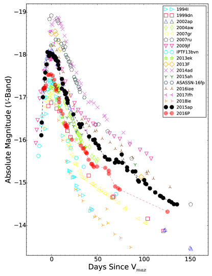
Figure 5: Absolute magnitude $V$-band light curves of SNe 2015ap and 2016P compared to other members of the sub-class. The light-curves have been corrected for distance and extinction given in Table 2.

Figure 5 shows the absolute magnitude light curves of SNe 2015ap and 2016P along with other members of the sub-class which are corrected for extinction and reddening values reported in Table 2. The peak absolute magnitudes of SNe 2015ap and 2016P are listed in Table 1. The absolute magnitudes of SN 2015ap in $V$ and $R$-bands are $-$18.04 $\pm$ 0.19 mag and $-$18.15 $\pm$ 0.17 mag, respectively, which are comparable with the average distribution of Type Ib SNe ($-$17.98 $\pm$ 0.13 mag; Richardson et al., 2006, $-$17.9 $\pm$ 0.9 mag; Drout et al., 2011). As compared with the recent results by Taddia et al. (2018), the average value of Type Ib SNe to be $-$17.07 $\pm$ 0.56, $V$-band absolute magnitude of SN 2015ap is brighter by $\sim$ 0.5 mag. The $V$-band absolute magnitude light curve of SN 2015ap shows that it is one of the bright SN among the Type Ib SNe used for comparison. The $R$-band absolute magnitude of SN 2016P is $\sim$ 0.5 mag fainter than the sample of Type Ic SNe ($-$18.3 $\pm$ 0.6; Drout et al., 2011). The $V$-band absolute magnitude is also fainter than the sample of Type Ic by 1 mag ($-$18.51 $\pm$ 0.10 mag; Richardson et al., 2006) while the values are consistent with the recent results by Taddia et al. (2018). Table 2 shows that SN 2015ap lies among the brighter end of the Type Ib comparison sample while SN 2016P is of average brightness object among the Type Ic comparison sample.

We constructed the bolometric light curves of SNe 2015ap and 2016P using black-body (BB) fitting model. The bolometric lightcurves were constructed by using the photometric data of at least 3 filters to fit black-body spectral energy distribution (SED). For SN 2015ap, however, we also used the pre-peak data of 2 filters since we need pre-peak bolometric lightcurve to pose more stringent constraint on the explosion epoch. Neglecting the dilution effect of the ejecta (Dessart et al., 2012) and assuming that the SN emission is mostly blackbody, we estimated the blackbody temperature (T) and photospheric radius (R_ph) as free parameters of our code. We neglect the blue-ultraviolet (UV) suppression that yields lower UV and bright optical luminosities. Using the values of T and R_ph, obtained through BB fitting and considering the contribution of far-UV and far-IR emission, we estimated the bolometric luminosities using the formula 4$\pi$R${}_{\rm ph}^{2}$$\sigma$T⁴. However, in reality, the spectra of SNe Ib/c are not black bodies and there is substantial deviation from this at early and late times due to line blanketing and line emission/loss of photosphere respectively. With the assumption that the photospheric velocity (v_ph) is equal to the scale velocity (v_sc), we have modelled the light curves of both the SNe. The photospheric velocity values are taken from the SYN++ modelling of the spectrum done in Sec 5. We have constrained the priors in the code to obtain physical values of the obtained parameters. In order to fit the bolometric light curves of SNe 2015ap and 2016P, we used Markov Chain Monte-Carlo (MCMC) simulations on the light curves to obtain the best-fit parameters. The optical opacity is fixed to be 0.07 cm² g^-1 which is justified if electron scattering opacity is the dominant source (see for example Taddia et al. 2018).

⁵⁶Ni model: With the assumption that the bolometric luminosity is powered by the decay of ⁵⁶Ni to ⁵⁶Co and ⁵⁶Co to ⁵⁶Fe, we fit the bolometric light curves using the ⁵⁶Ni model. The ⁵⁶Ni model was constructed taking into account the assumptions of Arnett (1982) and Chatzopoulos et al. (2012). The employed free parameters of ⁵⁶Ni model are the ejecta mass M_ej, ⁵⁶Ni mass M_Ni, gamma-ray opacity of ⁵⁶Ni decay photons $\kappa$_γ,Ni and explosion time t_expl. Following Arnett (1982), $\tau_{m}$ determines the width of the bolometric light curve and can be expressed in terms of opacity ($\kappa$), ejecta mass M_ej, and the photospheric velocity at luminosity peak v_ph:

$$\tau_{m}=\sqrt{2}{\bigg{(}\frac{k}{\beta c}\bigg{)}^{\frac{1}{2}}}{\bigg{(}\frac{M_{\rm ej}}{v_{\rm ph}}\bigg{)}^{\frac{1}{2}}}$$ (1)

where $\beta=13.8$ is a constant of integration (Arnett, 1982) and c is the speed of light. The kinetic energy for spherically symmetric ejecta with uniform density is:

$$E_{k}=\frac{3}{10}M_{\rm ej}v_{\rm ph}^{2}$$ (2)

The best-fit parameters of the model are tabulated in Table 4 and the best-fit ⁵⁶Ni model of SNe 2015ap and 2016P are displayed in Fig 6. The associated corner plots showing confidence level of different parameters are shown in Fig 7 and Fig 8, respectively. For SN 2015ap, the ⁵⁶Ni model is able to reproduce the peak luminosity however it underestimates the luminosity at late times. Similarly, for SN 2016P the ⁵⁶Ni model fails to reproduce the luminosity around peak and is a good match to the observed data at late times. In both the SNe, this indicates that ⁵⁶Ni may not alone be the powering source and an additional source of energy is required to generate the observed luminosity.

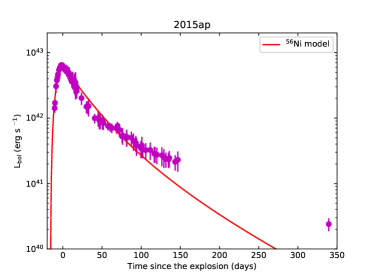
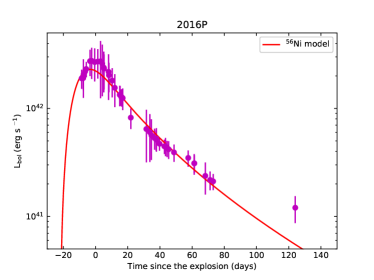
Figure 6: The bolometric light curves of SNe 2015ap (the left panel) and 2016P (the right panel) reproduced by the ⁵⁶Ni model. The abscissa represents time since the explosion in rest frame. The open circles are derived using two band data while filled circles are derived using three or four band data.

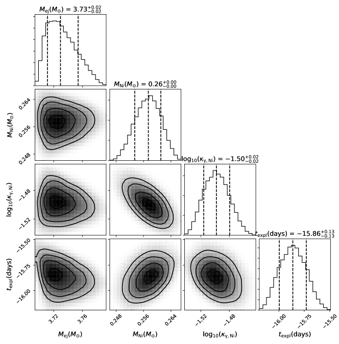
Figure 7: Corner plot of SN 2015ap showing the parameters (M_ej, M_Ni, $\kappa_{\rm\gamma}$, t_expl) of the ⁵⁶Ni model.

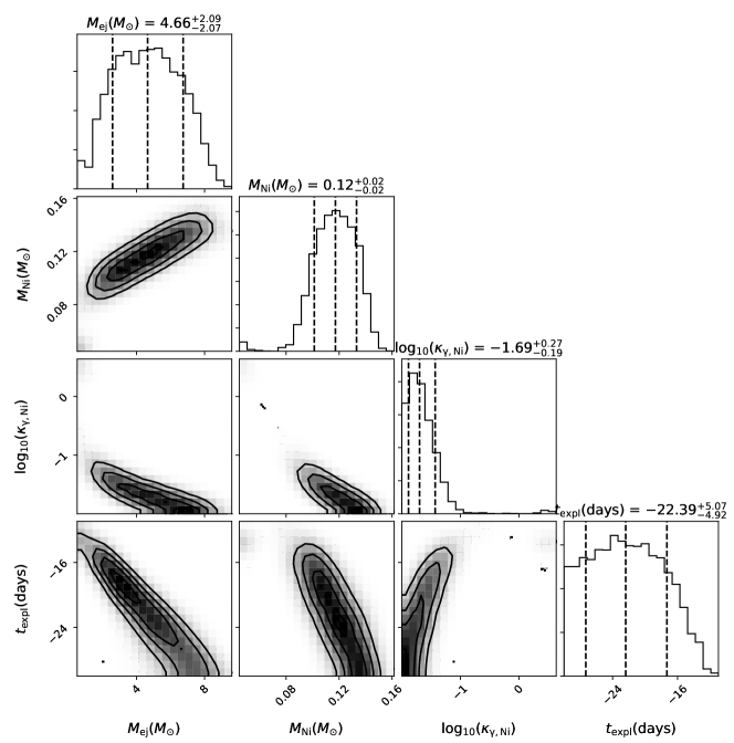
Figure 8: Corner plot of SN 2016P showing the parameters (M_ej, M_Ni, $\kappa_{\rm\gamma}$, t_expl) of the ⁵⁶Ni model.

Table 4: Parameters of the various models. The uncertainties are 1$\sigma$.

	$\kappa$	$v_{\mathrm{sc}}$	$M_{\mathrm{ej}}$	$M_{\mathrm{Ni}}$	$P_{0}$	$B_{p}$	$\kappa_{\gamma,\mathrm{Ni}}$	$\kappa_{\gamma,\mathrm{mag}}$	$t_{\mathrm{expl}}$⋆	$\chi^{2}/\mathrm{dof}$
	(cm2 g-1)	($10^{9}$cm s-1)	(M⊙)	(M⊙)	(ms)	($10^{14}$ G)	(cm2 g-1)	(cm2 g-1)	(days)
SN 2015ap
56Ni	0.07	1.6	$3.73^{+0.02}_{-0.02}$	$0.26^{+0.00}_{-0.00}$	-	-	$0.032^{+0.001}_{-0.001}$	-	$-15.86^{+0.13}_{-0.13}$	113.64/72
magnetar+56Ni	0.07	1.6	$3.90^{+0.21}_{-0.15}$	$0.01^{+0.00}_{-0.00}$	$25.85^{+0.50}_{-0.67}$	$28.39^{+1.64}_{-1.66}$	$0.26^{+0.05}_{-0.04}$	$14.26^{+24.59}_{-8.49}$	$-13.17^{+0.20}_{-0.21}$	10.87/69
SN 2016P
56Ni	0.07	1.5	$4.66^{+2.09}_{-2.07}$	$0.12^{+0.02}_{-0.02}$	-	-	$0.02^{+0.02}_{-0.01}$	-	$-22.39^{+5.07}_{-4.92}$	12.57/38
magnetar+56Ni	0.07	1.5	$5.13^{+1.03}_{-1.03}$	$0.002^{+0.006}_{-0.004}$	$36.51^{+2.16}_{-2.31}$	$35.30^{+5.25}_{-3.60}$	$1.82^{+17.94}_{-1.66}$	$1.19^{+13.09}_{-1.11}$	$-16.31^{+1.32}_{-1.47}$	3.18/35

$\star$ The value of $t_{\mathrm{expl}}$ is with respect to the date of the first $R$-band observation; the lower limit is set to be $-30$ here.

⁵⁶Ni + Magnetar model: One of the most prevailing model adopted to model the light curves of SNe that cannot be explained by the ⁵⁶Ni model is the magnetar model (Inserra et al., 2013; Wang et al., 2015a). However, as pointed out by Nomoto et al. (2013), the core-collapse SNe can yield $\leq$ 0.2 M_⊙ of ⁵⁶Ni and the luminosity produced by ⁵⁶Ni decay cannot be neglected in modeling the SNe whose peak luminosities are not very high. Therefore, a hybrid model taking into account the contribution from a newly born magnetar and a moderate amount of ⁵⁶Ni could be a promising model for SNe 2015ap and 2016P. We try to fit the light curves of both SNe 2015ap and 2016P using the ⁵⁶Ni + Magnetar model (Wang et al., 2015b). The free parameters of the ⁵⁶Ni + magnetar model are $\kappa$, M_ej, magnetic field B_p, the initial rotational period P₀, the gamma-ray opacity of magnetar photons $\kappa$_γ,mag, the gamma-ray opacity of ⁵⁶Ni cascade decay photons $\kappa$_γ,mag, and t_expl.

The best-fit light curves are shown in Fig 9 and the parameters are tabulated in Table 4. The associated corner plots showing confidence level of different parameters are also shown in Fig 10 and Fig 11 respectively. Even though the obtained ⁵⁶Ni mass is low as compared to its kinetic energy, the ⁵⁶Ni + magnetar model shows good fits to the overall light curves of both the SNe. The uncertainties and the confidence of determination of the parameters as well as the degeneracy and correlation between parameters are shown in the corner plots. However, we remark that the values of ejected mass and the derived kinetic energy depend on the adopted value of opacity.

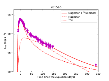
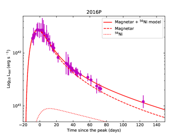
Figure 9: The bolometric light curves of SNe 2015ap (the left panel) and 2016P (the right panel) reproduced by the Magnetar + ⁵⁶Ni model (the right panel). The abscissa represents time since the explosion in rest frame.

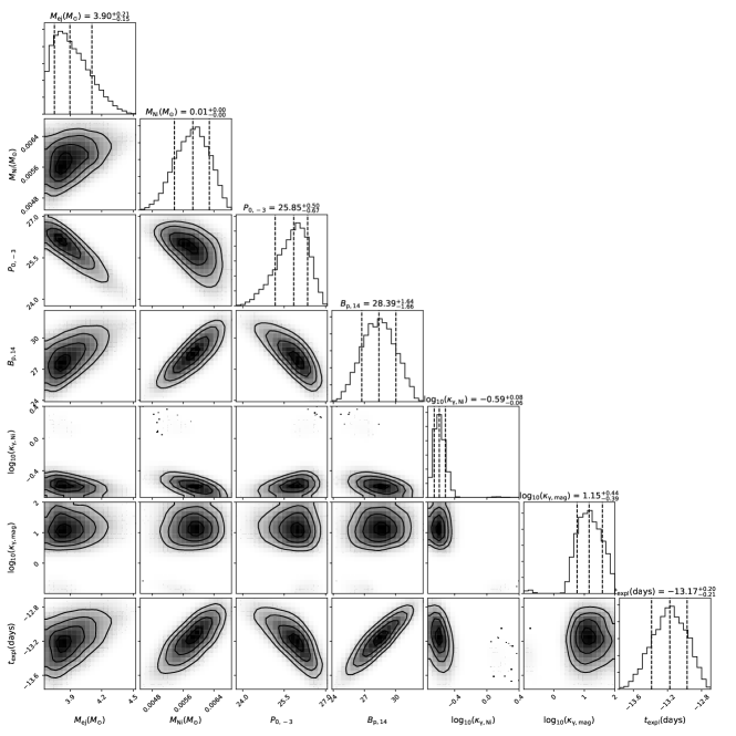
Figure 10: Corner plot of SN 2015ap showing the parameters (M_ej, M_Ni, P₀, B_p, $\kappa_{\rm\gamma,Ni}$, $\kappa_{\rm\gamma,mag}$, t_expl) of the ⁵⁶Ni + magnetar model.

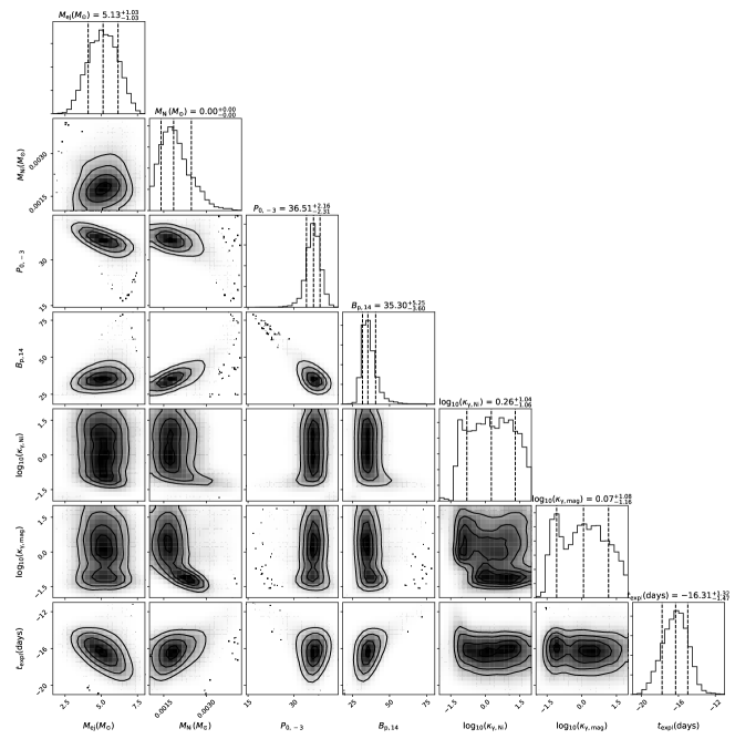
Figure 11: Corner plot of SN 2016P showing the parameters (M_ej, M_Ni, P₀, B_p, $\kappa_{\rm\gamma,Ni}$, $\kappa_{\rm\gamma,mag}$, t_expl) of the ⁵⁶Ni + magnetar model.

5 Spectroscopic evolution

Our spectroscopic observations of SN 2015ap started 14 days before $V$-maximum and continued upto 125 days post-maximum while the spectral coverage of SN 2016P is limited to 28 day after $V$-maximum. We explain in detail the spectroscopic features of these two events below.

5.1 Spectral evolution of SNe 2015ap and 2016P during early phase

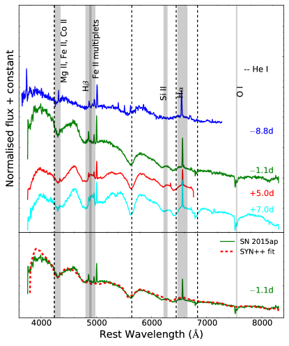
Figure 12: Early time spectral evolution of SN 2015ap. Prominent He features are seen in early spectra. The bottom panel shows the $-$1.1 day spectrum plotted along with the best fit model generated by SYN++(dotted lines). Prominent lines of He I are marked with vertical dashed black lines.

The pre-maximum spectral evolution of SN 2015ap is shown in Fig 12. The early time spectral sequence of SN 2015ap shows a blue continuum. Initial few spectra show distinct, blueshifted and broad P-cygni profiles which is indicative of very high velocities. However, we remark that since SN 2015ap exploded close to H II region, there is contamination of host C II and S II contamination lines. Moreover, around 5000 Å  we see significant contamination by H $\beta$ and [O III] galaxy lines. In the $-$1.1 day spectrum of SN 2015ap, He I 5876 Å  absorption feature expanding with a velocity of $\sim$ 15,500 km s^-1 is seen. Other prominent spectral features noticed in the early time spectra are Fe II between 4100 and 5000 Å; Si II/H$\alpha$ at $\sim$ 6250 Å  and OI 7774 Å. The He I 4471 Å  line is present but with a possible blend of Fe II complexes and Mg II 4481 Å. Except 5015 Å  feature, all other He I lines at 4471, 5876, 6678 and 7065 Å  are prominent. The spectra taken at 5 day and 7 day of SN 2015ap in Fig 12 show “W" shape absorption feature around 4000 Å. Similar kind of feature was observed in Type II SN 2005ap (Quimby et al., 2007), Type Ib SN 2008D (Modjaz et al., 2009), SN 2009jf (Sahu et al., 2011) and Type IIb SN 2001ig (Silverman et al., 2009) but at very early epochs (between $-$14 day to $-$10 day). While Mazzali et al. (2008) claim the origin of this feature due to Fe complexes, Modjaz et al. (2009); Silverman et al. (2009) consider this feature to be originated due to C III, N III and O III lines at high velocities. Since we see the feature in post-maximum phases, we consider the feature to be originated due to Fe complex with a blend of Mg II. The observed spectrum of SN 2015ap is compared with a synthetic spectrum generated using SYN++ (Thomas et al., 2011) as shown in the bottom panel of Fig 12. The synthetic spectrum with photospheric temperature of 13,000 K and photospheric velocity v_ph = 16,000 km s^-1 reproduces the spectrum of SN 2015ap obtained at $-$1.1 day. The He I lines are moving with an expansion velocity of $\sim$ 15,500 km s^-1. Prentice et al. (2019) also estimated the He I 5876 Å  line velocities between $-$ 10 days to 20 days post bolometric maximum which varied between 16,000 km s^-1 to 11,000 km s^-1 which is in agreement with our results. We performed a blackbody fit on the $-$ 1.1 day spectrum of SN 2015ap resulting in a temperature estimate of 12,000 $\pm$ 2,000 K. Prentice et al. (2019) also estimated the temperature variations between $-$10 days to 40 days post bolometric maximum and found those to vary between 11,000 K to 5,000 K. Their estimated value of temperature are well within the errors of our estimates using blackbody fit.

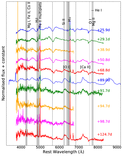
Figure 13: Spectral evolution of SN 2015ap between 25 to 124 day post $V$-maximum. Post 70 days, the [O I] and [Ca II] features start dominating.

Fig 13 shows the evolution of SN 2015ap from 26 day to 124 day post maximum. We see that the broad He I absorption feature has decreased with time. Also, the blue continuum has decreased implying a decrease in photospheric temperature. All other spectral lines become prominent and well-developed. The He I line around 5876 Å  may be blended with Na I 5890, 5896 Å. Post 90 day, we see distinct [O I] 6300, 6364 Å  doublet in the spectra of SN 2015ap which marks the onset of nebular phase. We notice prominent [O I] 6300, 6364 Å  and [Ca II] 7291, 7324 Å  doublet feature in Fig 13 after this phase. Other identified lines in the spectra include Mg I] 4571 Å  feature, OI 7774 Å  blended with contributions from OI 8446 Å. We see multipeaked [O I] in the nebular phase spectra of SN 2015ap which is indicative of a highly asymmetric ejecta configuration which will be discussed in detail in Section 6.

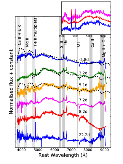
Figure 14: Spectral evolution of SN 2016P. Dotted lines in the first three spectra show the best fit SYN++ model. The shaded region at 5100 Å  in the inset plot shows a shallow feature of unknown origin.

Fig 14 shows spectral sequence of SN 2016P covering a phase range of -5 to 22 days post $V$-maximum. The 0.1 day spectrum shows a blue continuum. Prominent lines of Mg II, multiplets of Fe II, Si II, O I and Ca II NIR features are seen in the spectrum. In the spectral sequence, we see two shallow absorption feature at 5100 Å  and 5500 Å. The shallow absorption at 5150 Å  was noticed as an unidentified feature for Type Ic SN 2004aw (Taubenberger et al., 2006). The broad absorption feature post 6000 Å  is believed to have several origins. The feature is thought to be associated with Si II 6355 Å  (Foley et al., 2003; Valenti et al., 2008a; Hunter et al., 2009; Sahu et al., 2009; Pignata et al., 2011; Kumar et al., 2018). This absorption feature is also seen in SN 2007gr (Valenti et al., 2008b), SN 2004aw (Taubenberger et al., 2006) and SN 2013ge (Drout et al., 2016). For SNe 2004aw and 2013ge, the feature is considered due to C II 6580 Å. The absorption dip at 5500 Å  may result from a possible blending of Na I along with He I features (Pandey et al., 2003; Valenti et al., 2008a; Sahu et al., 2009). To the first three spectra of SN 2016P, we fit SYN++ model. The dotted lines in Fig 14 shows the best-fit SYN++ model that is moving with a photospheric velocity of v_ph = 15,000 km s^-1 and temperature of 8000 K which fits the first spectrum well. As we move to the third spectrum, v_ph = 13,000 km s^-1 is achieved with temperatures reaching upto 7000 K. Prentice et al. (2019) also show that at similar epochs, photospheric temperature of SN 2016P is 8,000 K. Prominent lines of Si II, Fe multiplets and Ca lines are also well reproduced. Si II lines show a velocity of 10,000 km s^-1 well in agreement with Prentice et al. (2019).

5.2 Spectral comparison among SE-SNe

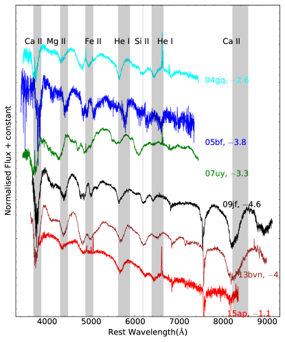
Figure 15: Spectral comparison of SN 2015ap along with other Type Ib SNe. SN 2015ap shows a distinct blue continuum.

The comparison of the pre-maximum spectrum of SN 2015ap is shown in Fig 15. The $-$1.1 d spectrum of SN 2015ap shows a distinct blue continuum as compared to all other SNe indicating higher temperatures. This is also in agreement with the results reproduced by SYN++ fitting. He I absorption lines are well established in all the spectra.

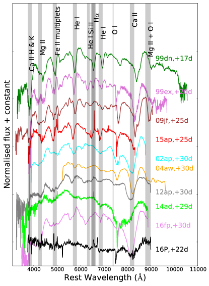
Figure 16: Spectral comparison of SNe 2015ap and 2016P at $\sim$ 25 day post $V$-maximum with other SNe. The overall spectrum of SNe 2015ap and 2016P shows resemblance with SNe 2009jf and 2012ap respectively.

We compare the $\sim$ 25 day spectra of SNe 2015ap and 2016P with a number of Ib, Ic, Ic-BL and transitional Ic SNe in Fig 16. The spectrum of SN 2015ap bears a close resemblance with SN 2009jf. Prominent He I 5876 Å  features are seen in the whole sample of Type Ib SN. The He I features in SN 2015ap are very similar to SN 2009jf. The overall spectrum of SN 2016P (at 22 day) is quite similar to SN 2012ap. Prominent Mg II features at other wavelengths along with Mg II + O I at 9000 Å  is well-developed as compared to all other SNe of the comparison sample. The absorption dip close to 6200 Å  is also found to be similar to that of SN 2012ap. The overall spectra of SN 2016P shows lines having width in between Type Ic and Ic-BL SNe.

Figure 17: Nebular phase comparison of SN 2015ap shows less prominent emission peaks than other SNe. SN 2015ap shows distinct multi-peaked profiles of [O I] different from all other SNe.

Fig. 17 shows the nebular phase comparison spectra of SN 2015ap along with other Type Ib SNe. SN 2015ap shows an asymmetric emission profile of [O I] as compared to other SNe. Also, the [Ca II] doublet is broad and dispersed than others. This has several implications on the physical scenario which we will explain in detail in Section 6.

6 Asymmetry in the nebular phase emission of SN 2015ap

As the nebular phase probes deeper into the ejecta, several studies on the ejecta geometry and associated asymmetries have been done in the past (Mazzali et al., 2005; Maeda et al., 2008; Modjaz et al., 2008; Taubenberger et al., 2009; Milisavljevic et al., 2010). The most-prominent lines in nebular phase to study ejecta geometry are [O I] 6300, 6364 Å  doublet, [Ca II] 7291, 7324 Å  doublet and the Mg I] 4571 Å  lines. However, [O I] is best to probe asymmetry as [Ca II] lines may be contaminated with [O II] 7320, 7330 Å  (Fesen et al., 1999) lines and Mg I] line is contaminated by Fe lines. Also, oxygen is the most abundant element in the SN ejecta and forms in a wavelength region where sensitivity of most of the spectrographs is maximum. The ratio of [O I] 6300/6364 Å  lines changes from 1:1 to 3:1 for H-rich SNe when the density limit approaches 10¹⁰ cm^-3 (Leibundgut et al., 1991; Pinto & Spyromilio, 1991; Chugai, 1992). While Taubenberger et al. (2009) suggested that during nebular phase, the ratio is always 3:1 for Type Ib SNe but Milisavljevic et al. (2010) argued that the ratio may be close to 1:1 in order to explain the dominance of double peaks in Type Ib rather than Type Ic. Maeda et al. (2006) used a ratio of 3:1 for their nucleosynthesis models which was observationally confirmed by Hunter et al. (2009) for SN 2007gr. Maurer et al. (2010) showed that high velocity H$\alpha$ absorption feature can be superimposed on the oxygen emission profiles giving rise to double peaks.

SN 2015ap has a complex oxygen profile with multiple peaks/asymmetric shifted from 6300 Å  as shown in Fig 18(A). We do not detect any Hydrogen features in SN 2015ap, so the high velocity feature as the reason for multi-peaked profile is ruled out. The spectrum has been smoothed using a boxcar factor of 9 to reduce the noise. The SNR of all the peaks was checked in the smoothed spectrum of 124 d and compared with the background. The overall spectrum has a SNR of about 4. We checked the SNR of the individual peaks and found that the peak at -1600 km/sec is of course real and is four times higher than the background, thus validating that the peak is real and hence confirming existence of an asymmetric profile. The other peaks are two times higher than the background. As we obtain a blueshifted peak, we interpret this as per Taubenberger et al. (2009) which explains blueshift being originated due to either suppression of the redshifted part of the spectrum as dust forms or residual opacity as ejecta cools. These kind of profiles have been seen previously in SNe 1990B, 1990aa, 1999dn, 2006F and 2009jf (Taubenberger et al., 2009). Taubenberger et al. (2009) explained these asymmetric profiles that are produced by additional components of arbitrary widths and shifts with respect to main component. This indicates clumping of the SN ejecta on a large scale. It may also be due to a single massive blob and a unipolar jet. However, to check the evolution of line profiles, we check this in the three additional spectra taken from WiseREP public archive and repeat the fitting procedure as discussed above. We find that the spectra of 124 d and 125 d are well fit with two Gaussians but the spectra of 128 d and 144 d are well fit with a single Gaussian (see Fig 19). This indicates a transition in the [O I] line profile, but an overall clumpiness and asymmetric ejecta configuration is seen in all the profiles.

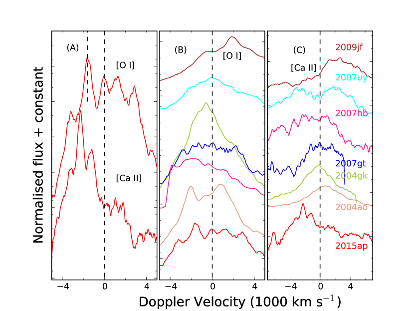
Figure 18: Panel (A) of the Fig represents the line profiles of [O I] 6300, 6364 Å  and [Ca II] 7291, 7324 Å. Panel (B) and (C) shows the comparison of the [O I] and [Ca II] profile of SNe 2015ap with other Type Ib/c SNe sample. The black dashed lines in Fig 18 (A) represents the zero velocity line corresponding to 6300 Å  and left line represents the real peak at -1600 km sec^-1. In panel (B), the black line represents the velocity corresponding to 6300 Å  and panel (C) represents the velocity corresponding to 7291 Å  line.

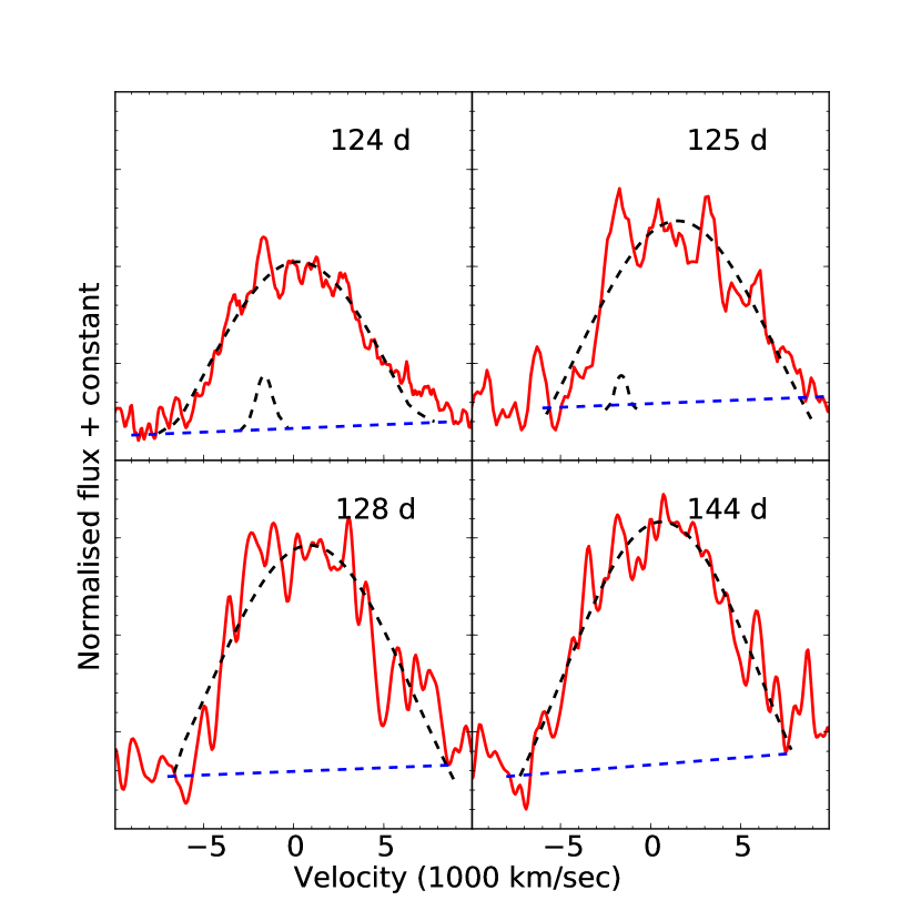
Figure 19: Oxygen profile of SN 2015ap fitted with Gaussian profiles. Top two panels shows two peaks while bottom two panels shows an overall asymmetric structure.

Fig 18(A) also displays the Ca II profile. We see a blueshifted prominent peak in the doublet. This has a similar origin as that of [O I] profile (Taubenberger et al., 2009). The overall variation is however smooth as compared to the [O I] emission. Clumps of Ca do form, but they do not contribute significantly to emission. These clumps of Ca intercept $\gamma$-ray radiation. However, as the mass fraction is small, the amount of radioactive luminosity and temperature achieved is not sufficient for the emission (Li et al., 1993; Matheson et al., 2000). The pre-existing envelope of the star is heated generally by hydrogen and helium that do not radiate efficiently, allowing Ca that was thoroughly mixed into the atmosphere, most likely present from the time of the progenitor formation, to reach the temperatures required to produce [Ca II] emission indicating a primordial origin.

Fig 18(B) and Fig 18(C) compares the spectrum of SN 2015ap with a number of Type Ib/c SNe (phase range - 110 to 150 day) that are taken from WiseREP public archive. We see that the [O I] profile of SN 2015ap bears a resemblance with SNe 2007gt and 2009jf while [Ca II] profile bears a close resemblance with SN 2007hb. The [O I] profile of SN 2015ap shows a clumpy profile as compared to the double peaked and single peaked profile of most of the other SNe. This may be due to the different geometrical orientation of the [O I] in different SN ejecta. If we look into the [Ca II] profiles, the profiles of all the Type Ib SNe have clumpiness less than the [O I] profiles. This may be due to the fact that the amount of primordial Calcium is more than the [Ca II] that are generated during the nucleosynthesis process going on in the SN evolution.

6.1 Estimates of the O mass and [O I] / [Ca II] ratio

The line strengths in the nebular phase spectra provide key information on the progenitor mass. Uomoto & Kirshner (1986) derived a relation, showing the minimum mass of O that can be estimated in the high density (N_e $\geq$ 10⁶ cm^-3) limit (Schlegel & Kirshner, 1989; Elmhamdi et al., 2004). This is given by

$$M_{O}=10^{8}\times D^{2}\times F([O\,I])\times exp^{(2.28/T_{4})},$$ (3)

where $M_{O}$ is the mass of the neutral O in M_⊙ units, $D$ is distance to the galaxy in Mpc, $F([OI])$ is the total flux of the [O I] 6300, 6364 Å  feature in erg s^-1 cm^-2, and $T_{4}$ is the temperature of the O-emitting region in units of 10⁴ K. Ideally, the ratio of [O I] 5577 Å to the [O I] 6300, 6364 Å  feature should be considered. Osterbrock (1989) showed that the ratio of [O I] 5577 Å  to [O I ] 6300 is proportional to the electron density and the temperature of the emitting regions. Thus, the uncertainties associated in the equation are large which involves the errors due to the flux, temperature and indirectly the density. The temperatures can typically vary between (0.4 – 1) x 10⁴ K. We find that the [O I] 5577 Å  line is very faint, and the limit of the flux ratio is $\leq$ 0.1. Using the observed flux of 3.0 x 10^-14 erg s^-1 cm^-2 of the [O I] 6300, 6364 Å  doublet from the 2016 January 22 spectrum, and adopting T₄ = 0.4 K, we estimate $M_{O}$ = 0.90 M_⊙. A very weak OI 7774 Å  emission feature is seen in the nebular spectra. Since the O I 7774 line is expected to result from recombination of ionized O (Begelman & Sarazin, 1986), the O mass required to produce the [O I] doublet and the O I 7774 Å  line is higher than the mass required to produce the doublet alone (Mazzali et al., 2010). Therefore, 0.90 M_⊙ can be considered as a lower limit of total oxygen mass ejected in the explosion. [O I] layer is mostly produced by hydrostatic burning of oxygen. Thielemann et al. (1996) made explosive nucleosynthesis calculations and predicted major nucleosynthesis yields for the progenitor mass of 13 $-$ 25 M_⊙. For progenitor masses of 13, 15, 20 and 25 M_⊙, Thielemann et al. (1996) showed that the corresponding O masses would be 0.22, 0.43, 1.48 and 3.0 M_⊙, respectively. Also, Thielemann et al. (1996) estimated He core masses of 3.3, 4 and 8 M_⊙, corresponding to progenitors of 13, 15 and 25 M_⊙, respectively. Thus, using this model and corresponding approximations we conclude that the progenitor of SN 2015ap is most likely a star between 15 $-$ 20 M_⊙ and He core mass between 4 $-$ 8 M_⊙.

Kuncarayakti et al. (2015) estimated the value of [O I]/[Ca II] ratio for a group of core-collapse SNe and found that this ratio is highly dependent on temperature, density and progenitor mass. Kuncarayakti et al. (2015) considered a demarcation of SNe progenitors as binary and single if this ratio was lower or higher than 1.5 respectively. However, this ratio is close to 0.7 for Type IIP SNe. In the case of SN 2015ap the [O I]/[Ca II] ratio is $\sim$ 0.71 indicating that the progenitor is a low mass star in a binary system.

6.2 Progenitor mass from oxygen line luminosities

The observed strength of the nebular lines can serve as an important diagnostic of the progenitor mass. Jerkstrand et al. (2012); Jerkstrand et al. (2014) generated nucleosynthesis models for progenitor masses of 12, 15, 19 and 25 M_⊙, assuming ⁵⁶Ni mass to be 0.062 M_⊙ and distance of 5.5 Mpc for a group of Type IIP SN. Jerkstrand et al. (2015) extended this for a group of SE-SNe by implementing minor modifications in the code. They generated three models of 12, 13 and 17 M_⊙ for the stripped envelope group with ⁵⁶Ni mass = 0.079 M_⊙ and distance of 7.9 Mpc. In Fig 20, we compare the 137 day post explosion (or 124 day since $V$-maximum) spectrum of SN 2015ap with the 150 day and 12, 13 and 17 M_⊙ model generated by Jerkstrand et al. (2015) for Type IIb/Ib SNe. It is to be noted that the model assumes elemental abundances which are higher than the estimates of for lower progenitor mass.

We modelled the spectra of SN 2015ap adopting a ratio of (0.26/0.079) to correct ⁵⁶Ni mass and rescale the model flux (150 d) to the distance and phase of the (137 day) nebular spectrum of SN 2015ap. The SN spectrum is de-reddened and de-redshifted to avoid any flux loss before comparison. We see that the overall spectrum matches better with a 12 M_⊙ progenitor star. We then, subtracted the host galaxy spectrum taken from SDSS DR14 of SN 2015ap from the SN spectrum. Fig 20 shows both the subtracted and unsubtracted spectrum of SN 2015ap. The galaxy lines of H and S II are removed in this spectrum and also there is an overall flux decrement, implying a progenitor of mass less than 12 M_⊙. It is to remark, however, that these models assumes an over abundance of elements as compared with Thielemann et al. (1996), so a lower progenitor mass would indicate an over estimated peak. Also, due to the high density envelope used in the model, scattering of other lines may affect the flux estimations. The [O I] feature matches well with a 12 M_⊙ progenitor star for the unsubtracted spectrum. Our obtained value of L_norm = 0.015 which is a good tracer of L_[OI] (Jerkstrand et al., 2015) matches well with the value estimated by Prentice et al. (2019). Comparing the line luminosities of [O I] and the fitted nebular spectral modeling indicates that the progenitor of SN 2015ap is in the range of 12 $-$ 20 M_⊙ which is most likely in a binary association.

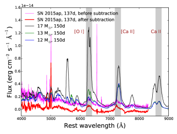
Figure 20: The 137 day since explosion spectrum of SN 2015ap plotted along with the 12, 13 and 17 M_⊙ models of Jerkstand et al. 2015 at 150 day. The 12 M_⊙ model best matches our observed spectrum of SN 2015ap.

6.3 Host galaxy metallicity

Metallicity is a key parameter driving mass-loss rates in single stars and influences the relative number of Type Ib/c SNe. It’s also important for binary models (Eldridge et al., 2008) and affects the ratios of Type Ib/c SNe. In order to estimate the host galaxy metallicity, we used the Sloan Digital Sky Survey (SDSS) spectrum of IC 1776; the host galaxy of SN 2015ap. The DR12 SDSS image was taken on 2010 November 13. Narrow emission lines of [O III] 5007 Å  and the [N II] 6583 Å  lines are clearly visible in the host galaxy spectrum. Several diagnostics are used to estimate the host galaxy metallicity (McGaugh, 1991; Kewley & Dopita, 2002; Pettini & Pagel, 2004; Pilyugin & Thuan, 2005). We used the O3N2 index calibration given by Pettini & Pagel (2004) to estimate the host galaxy metallicity. The value of 12 + log(O/H) is found to be 8.8 $\pm$ 0.6 dex. For SN 2016P, the SDSS DR12 image of the galaxy NGC 5374 was taken on 2007 March 16. In this spectrum also, narrow emission lines of [O III] 5007 Å  and the [N II] 6583 Å  were seen. The value of 12 + log(O/H) for NGC 5374 is found to be 8.7 $\pm$ 0.5 dex. Several authors have estimated the solar metallicity values to be 8.69 $\pm$ 0.05 dex, 8.69 dex and 8.76 $\pm$ 0.07 dex, (Allende Prieto et al., 2001; Asplund et al., 2009; Caffau et al., 2011) The obtained metallicity value for IC 1776 is slightly super-solar while NGC 5374 has nearly solar metallicity. However, the metallicity is close to solar for both the galaxies within errors. Wolf-Rayet progenitor could be one of the favourable scenario as the number of WR stars increases with increasing metallicity due to the strong metallicity dependence on stellar winds (Vink & de Koter, 2005; López-Sánchez & Esteban, 2010). The progenitors could be in the form of either single WR stars or in binary association. Galbany et al. (2016) estimated the metallicity of a group of Type II and Ib/c SNe and found an average metallicity of 8.50 dex with an error of 0.02 for all SNe. Their results support a binary progenitor for SNe Ib and at least a fraction of SNe Ic to be single massive stars that have stripped their outer layers by metallicity driven winds.

7 Summary

In this paper, we present the temporal and spectral evolution of a Type Ib SN 2015ap and a Type Ic SN 2016P. The early decline rates of SNe 2015ap and 2016P are consistent with other Type Ib/c SNe while the late time light curves of both the SNe shows steepening. The colours of SN 2015ap are similar to most Type Ib comparison sample while the colour evolution of SN 2016P is redder than most of the members. The absolute magnitude (M_V = $-$18.04 $\pm$ 0.19 mag) of SN 2015ap indicates that it lies at the brighter end of Type Ib SN among the comparison sample while SN 2016P lies in the middle (M_V = $-$17.53 $\pm$ 0.14 mag) among Type Ic sample. The bolometric light curve modelling of SNe 2015ap and 2016P indicates that the light curves can be best fit by a ⁵⁶Ni + magnetar model with ⁵⁶Ni masses of 0.01 M_⊙ and 0.002 M_⊙, ejecta masses of 3.75 M_⊙ and 4.66 M_⊙, spin period P₀ of 25.8 ms and 36.5 ms and magnetic field B_p of 28.39 $\times$ 10¹⁴ Gauss and 35.3 $\times$ 10¹⁴ Gauss respectively. We suspected an additional energy source from a newly born magnetar because of the inability to fit the late time light curves and high luminosity. The narrow light curve and short rise time for SN 2015ap implied that the high ejecta mass is most likely a resultant of terminal fallback.

Early time spectral sequence of SN 2015ap shows prominent He I absorption lines with a blue continuum and high photospheric temperature. SYN++ modelling of the early time spectra of SN 2015ap indicates a photospheric temperature of 13,000 K and a photospheric velocity of 16,000 km s¹. Initial spectral sequence shows a “W" like feature arising due to Fe complexes. SN 2016P shows prominent lines of Ca II H $\&$ K, Mg II, Fe II and Ca II NIR features. The broad absorption blueward of 6000 Å  mostly arises due to a blend of Si II and C II. SYN++ modelling gives an initial photospheric velocity v_ph = 15,000 km s^-1 and temperature of 8000 K.

The [O I] profile of SN 2015ap shows an asymmetric profile which is indicative of large scale clumping or a unipolar jet. The [O I] and [Ca II] doublet shows blueshifted peak originating from residual opacity or dust formation. [Ca II] envelope has an origin of pre-SN envelope. The estimated O mass is found to be 0.90 M_⊙. The [O I]/[Ca II] ratio and the Jerkstrand modelling indicates a progenitor of mass between 12 $-$ 20 M_⊙ and most likely in binary association (Sana et al., 2011).

Appendix A Photometry

In addition to the ground based telescopes, SN 2015ap was observed with Swift UVOT (Gehrels, 2004a, b; Roming et al., 2005) from 2015 September 09 to 2015 October 06. We take the Swift early UBV magnitudes from the Swift Optical/Ultraviolet Supernova Archive (SOUSA; Brown et al., 2014) and tabulate them in Table 7.

The SNe instrumental magnitudes were calibrated with respect to the local standards in the SN field. Three Landolt standard fields PG 2331, PG 0918 and PG 0231 were observed along with the SNe fields with HFOSC/HCT to generate a sequence of local standards. The observations were carried out at different altitudes with airmass varying between 1.1$-$2.0 with a typical seeing of $\leq$ 2 arcsec in $V$-band. The instrumental and catalogue magnitudes of Landolt field stars were fitted, using the least square regression technique, to estimate the zero points and colour term using a set of transformation equations (Stetson, 1992). Site extinction values, taken from Stalin et al. (2008), were used for the different filters. A root-mean-squared (rms) scatter between transformed and standard magnitude of Landolt stars was found to be between 0.02 – 0.05 mag in the UBVRI bands. Using the above zero points and colour term, we calibrated the magnitudes of 5 to 6 non-variable local standards in both the SNe fields (Table 5 and Table 6). These secondary standards are used to calibrate the SNe instrumental magnitudes by applying nightly zero-points. The errors due to calibration and photometric measurement were added in quadrature to estimate the final error on the SNe magnitudes. Whereever required the uri magnitudes were converted to URI using the equations of Jordi et al. (2006). The final photometry of SNe 2015ap and 2016P is given in Table 7 and Table 8 respectively.

Table 5: Star ID and the magnitudes in UBVRI filters of the 5 secondary standards in the field of SN 2015ap

Star ID	$\alpha$	$\delta$	$U$	$B$	$V$	$R$	$I$
	(h:m:s)	(∘ ’ ”)	(mag)	(mag)	(mag)	(mag)	(mag)
1	02:05:08.19	+06:04:32.52	17.91 $\pm$ 0.09	17.843 $\pm$ 0.046	16.915 $\pm$ 0.056	16.712 $\pm$ 0.021	16.392 $\pm$ 0.442
2	02:05:07.31	+06:04:29.29	17.47 $\pm$ 0.04	16.887 $\pm$ 0.097	15.957 $\pm$ 0.081	15.604 $\pm$ 0.098	15.062 $\pm$ 0.101
3	02:05:06.96	+06:04:49.94	17.12 $\pm$ 0.03	16.495 $\pm$ 0.034	15.558 $\pm$ 0.089	15.406 $\pm$ 0.071	14.395 $\pm$ 0.098
4	02:05:19.97	+06:09:48.75	15.01 $\pm$ 0.02	13.685 $\pm$ 0.087	13.013 $\pm$ 0.091	12.712 $\pm$ 0.124	11.780 $\pm$ 0.142
5	02:05:14.45	+06:10:41.91	16.97 $\pm$ 0.04	15.742 $\pm$ 0.088	14.597 $\pm$ 0.129	14.106 $\pm$ 0.112	3.055 $\pm$ 0.073

Table 6: Star ID and the magnitudes in BVRI filters of the 6 secondary standards in the field of SN 2016P

Star ID	$\alpha$	$\delta$	$B$	$V$	$R$	$I$
	(h:m:s)	(∘ ’ ”)	(mag)	(mag)	(mag)	(mag)
1	13:57:39.13	+06:07:01.70	18.07 $\pm$ 0.01	17.49 $\pm$ 0.02	17.12 $\pm$ 0.01	16.79 $\pm$ 0.02
2	13:57:36.18	+06:02:00.43	16.94 $\pm$ 0.01	16.29 $\pm$ 0.01	15.87 $\pm$ 0.01	15.51 $\pm$ 0.01
3	13:57:30.03	+06:08:05.81	18.83 $\pm$ 0.02	17.33 $\pm$ 0.01	16.34 $\pm$ 0.01	15.37 $\pm$ 0.01
4	13:57:19.55	+06:07:23.04	17.39 $\pm$ 0.01	16.74 $\pm$ 0.01	16.32 $\pm$ 0.01	15.94 $\pm$ 0.01
5	13:57:23.44	+06:09:35.95	16.88 $\pm$ 0.01	16.34 $\pm$ 0.01	15.99 $\pm$ 0.01	15.67 $\pm$ 0.01
6	13:57:48.83	+06:06:52.69	17.31 $\pm$ 0.01	16.39 $\pm$ 0.01	15.83 $\pm$ 0.01	15.36 $\pm$ 0.01

Table 7: Photometry of SN 2015ap

MJD	$U$	$B$	$V$	$R$	$I$	Telescope
	(mag)	(mag)	(mag)	(mag)	(mag)
57282.47	15.04 $\pm$ 0.07	15.57 $\pm$ 0.06	15.29 $\pm$ 0.09	—	—	HCT
57283.84	15.17 $\pm$ 0.06	15.63 $\pm$ 0.05	15.23 $\pm$ 0.01	15.14 $\pm$ 0.01	14.87 $\pm$ 0.01	HCT
57289.54	16.02 $\pm$ 0.08	15.94 $\pm$ 0.06	15.38 $\pm$ 0.06	—	—	ST
57290.23	—	16.43 $\pm$ 0.06	15.39 $\pm$ 0.06	15.15 $\pm$ 0.01	14.82 $\pm$ 0.01	HCT
57292.44	—	16.51 $\pm$ 0.01	15.55 $\pm$ 0.07	15.23 $\pm$ 0.01	14.85 $\pm$ 0.03	HCT
57298.92	17.84 $\pm$ 0.19	17.28 $\pm$ 0.09	16.12 $\pm$ 0.08	15.66 $\pm$ 0.01	15.24 $\pm$ 0.01	ST
57299.83	—	17.30 $\pm$ 0.17	16.18 $\pm$ 0.01	15.72 $\pm$ 0.01	15.23 $\pm$ 0.01	ST
57300.92	—	—	16.15 $\pm$ 0.01	15.92 $\pm$ 0.01	15.44 $\pm$ 0.01	ST
57302.44	18.01 $\pm$ 0.23	17.61 $\pm$ 0.11	16.33 $\pm$ 0.03	15.92 $\pm$ 0.02	15.43 $\pm$ 0.02	ST
57317.86	—	—	16.89 $\pm$ 0.02	—	16.44 $\pm$ 0.01	ST
57325.75	—	—	17.18 $\pm$ 0.36	16.82 $\pm$ 0.01	16.63 $\pm$ 0.01	ST
57330.70	—	—	—	17.12 $\pm$ 0.01	16.84 $\pm$ 0.01	ST
57331.77	—	—	17.25 $\pm$ 0.05	17.16 $\pm$ 0.01	16.84 $\pm$ 0.01	ST
57332.78	—	—	17.33 $\pm$ 0.03	17.17 $\pm$ 0.02	16.85 $\pm$ 0.02	ST
57334.72	—	—	—	17.19 $\pm$ 0.02	16.95 $\pm$ 0.01	ST
57335.86	—	—	17.39 $\pm$ 0.05	17.19 $\pm$ 0.01	16.93 $\pm$ 0.02	ST
57336.83	—	—	17.45 $\pm$ 0.04	17.19 $\pm$ 0.02	16.94 $\pm$ 0.02	ST
57341.83	—	18.26 $\pm$ 0.01	—	—	—	DFOT
57342.87	—	—	17.66 $\pm$ 0.04	—	16.96 $\pm$ 0.02	DFOT
57345.81	—	—	17.72 $\pm$ 0.02	17.28 $\pm$ 0.01	17.07 $\pm$ 0.02	ST
57353.78	—	18.29 $\pm$ 0.02	17.494 $\pm$ 0.019	—	17.24 $\pm$ 0.08	HCT
57357.83	—	18.43 $\pm$ 0.03	17.79 $\pm$ 0.02	17.53 $\pm$ 0.02	—	HCT
57361.80	—	18.54 $\pm$ 0.08	17.79 $\pm$ 0.05	—	17.29 $\pm$ 0.01	ST
57366.95	19.04 $\pm$ 0.04	18.36 $\pm$ 0.07	17.91 $\pm$ 0.06	17.82 $\pm$ 0.06	17.39 $\pm$ 0.06	Copernico
57375.35	19.42 $\pm$ 0.08	18.61 $\pm$ 0.06	17.99 $\pm$ 0.09	17.95 $\pm$ 0.09	17.39 $\pm$ 0.09	DFOT
57386.69	—	—	18.28 $\pm$ 0.03	18.19 $\pm$ 0.02	17.70 $\pm$ 0.04	ST
57387.70	—	—	18.29 $\pm$ 0.16	18.19 $\pm$ 0.02	17.72 $\pm$ 0.05	ST
57390.62	—	—	—	18.26 $\pm$ 0.03	17.78 $\pm$ 0.06	ST
57391.68	—	—	18.39 $\pm$ 0.09	—	17.79 $\pm$ 0.05	ST
57392.68	—	—	18.02 $\pm$ 0.03	18.24 $\pm$ 0.04	17.80 $\pm$ 0.05	ST
57402.68	—	18.79 $\pm$ 0.09	18.58 $\pm$ 0.13	—	17.95 $\pm$ 0.05	DFOT
57403.68	—	18.78 $\pm$ 0.06	18.59 $\pm$ 0.14	18.31 $\pm$ 0.05	18.08 $\pm$ 0.05	DFOT
57412.59	—	18.88 $\pm$ 0.02	18.69 $\pm$ 0.03	18.50 $\pm$ 0.20	18.201 $\pm$ 0.07	HCT
57415.60	—	—	—	18.48 $\pm$ 0.04	18.28 $\pm$ 0.06	ST
57417.64	—	—	18.76 $\pm$ 0.13	18.49 $\pm$ 0.05	18.30 $\pm$ 0.06	ST
57429.59	—	—	18.79 $\pm$ 0.09	18.59 $\pm$ 0.05	18.55 $\pm$ 0.01	ST
57628.04	21.93 $\pm$ 0.09	21.50 $\pm$ 0.08	21.09 $\pm$ 0.08	20.95 $\pm$ 0.08	20.86 $\pm$ 0.08	Copernico

Table 8: Photometry of SN 2016P

MJD	$B$	$V$	$R$	$I$	Telescope
	(mag)	(mag)	(mag)	(mag)
57408.00	17.71 $\pm$ 0.05	16.98 $\pm$ 0.05	16.90 $\pm$ 0.03	16.74 $\pm$ 0.02	ST
57408.98	—	—	16.69 $\pm$ 0.01	16.72 $\pm$ 0.03	ST
57409.52	17.73 $\pm$ 0.09	16.98 $\pm$ 0.08	—	16.64 $\pm$ 0.02	ST
57410.91	17.47 $\pm$ 0.06	16.90 $\pm$ 0.01	16.63 $\pm$ 0.04	16.43 $\pm$ 0.01	HCT
57419.89	18.05 $\pm$ 0.08	16.89 $\pm$ 0.09	16.41 $\pm$ 0.08	16.19 $\pm$ 0.01	HCT
57420.99	—	—	16.44 $\pm$ 0.01	16.19 $\pm$ 0.01	HCT
57422.02	—	17.02 $\pm$ 0.01	16.49 $\pm$ 0.02	16.24 $\pm$ 0.01	HCT
57424.98	—	17.21 $\pm$ 0.01	—	16.30 $\pm$ 0.01	HCT
57428.91	—	17.57 $\pm$ 0.05	16.99 $\pm$ 0.01	16.61 $\pm$ 0.03	ST
57432.00	—	17.80 $\pm$ 0.07	—	—	ST
57432.99	—	17.83 $\pm$ 0.09	17.21 $\pm$ 0.08	16.74 $\pm$ 0.06	ST
57433.89	19.02 $\pm$ 0.01	17.89 $\pm$ 0.09	17.35 $\pm$ 0.01	16.74 $\pm$ 0.01	HCT
57438.98	—	18.17 $\pm$ 0.01	17.73 $\pm$ 0.01	17.32 $\pm$ 0.03	HCT
57448.79	19.43 $\pm$ 0.01	18.31 $\pm$ 0.08	17.88 $\pm$ 0.01	17.81 $\pm$ 0.01	HCT
57451.50	19.45 $\pm$ 0.01	18.37 $\pm$ 0.07	17.99 $\pm$ 0.01	17.89 $\pm$ 0.01	HCT
57454.49	—	18.46 $\pm$ 0.09	18.05 $\pm$ 0.01	17.81 $\pm$ 0.01	DFOT
57454.74	—	18.49 $\pm$ 0.09	18.07 $\pm$ 0.01	17.86 $\pm$ 0.01	DFOT
57460.52	—	18.74 $\pm$ 0.09	18.23 $\pm$ 0.01	18.04 $\pm$ 0.02	HCT
57461.80	—-	18.78 $\pm$ 0.04	18.26 $\pm$ 0.01	18.07 $\pm$ 0.01	HCT
57462.84	19.58 $\pm$ 0.02	18.81 $\pm$ 0.02	18.26 $\pm$ 0.01	18.11 $\pm$ 0.08	ST
57465.90	—	—	18.30 $\pm$ 0.01	18.23 $\pm$ 0.02	ST
57478.32	—	19.00 $\pm$ 0.01	18.50 $\pm$ 0.01	18.51 $\pm$ 0.03	HCT
57485.54	—	19.26 $\pm$ 0.01	18.67 $\pm$ 0.01	—	HCT
57486.00	—	—	—	18.90 $\pm$ 0.02	DFOT
57489.50	20.12 $\pm$ 0.07	19.31 $\pm$ 0.07	18.93 $\pm$ 0.01	18.90 $\pm$ 0.01	DFOT
57491.41	20.18 $\pm$ 0.06	19.34 $\pm$ 0.01	18.99 $\pm$ 0.01	—	HCT
57510.77	—	—	19.04 $\pm$ 0.01	19.16 $\pm$ 0.23	ST
57542.67	—	19.86 $\pm$ 0.08	19.41 $\pm$ 0.09	19.59 $\pm$ 0.01	HCT

Table 9: Log of spectroscopic observations of SN 2015ap. The phase is measured with respect to $V$-maximum (MJD=57284.86$\pm$0.5).

Date	MJD	Phase	Telescope	Instrument	Range
					Å
2015/09/11	57276.06	-8.80	1.82m Copernico	AFOSC+gr04	3360-7740
2015/09/18	57283.75	-1.11	2.0m HCT	HFOSC+gr07+gr08	3800-6840,5800-8350
2015/09/24	57289.90	5.04	2.0m HCT	HFOSC+gr07	3800-6840
2015/09/26	57291.94	7.08	2.0m HCT	HFOSC+gr07+gr08	3800-6840,5800-8350
2015/10/08	57310.79	25.93	2.0m HCT	HFOSC+gr07+gr08	3800-6840,5800-8350
2015/10/19	57314.67	29.81	2.0m HCT	HFOSC+gr07+gr08	3800-6840,5800-8350
2015/10/28	57323.74	38.88	2.0m HCT	HFOSC+gr07	3800-6840
2015/11/09	57335.64	50.78	2.0m HCT	HFOSC+gr07+gr08	3800-6840,5800-8350
2015/11/27	57353.64	68.77	2.0m HCT	HFOSC+gr07+gr08	3800-6840,5800-8350
2015/12/17	57373.86	89.00	1.82m Copernico	AFOSC+VPH06/07	3200-10000
2015/12/20	57376.59	91.72	2.0m HCT	HFOSC+gr07+gr08	3800-6840,5800-8350
2015/12/23	57379.57	94.71	2.0m HCT	HFOSC+gr07	3800-6840
2015/12/27	57383.59	98.73	2.0m HCT	HFOSC+gr07+gr08	3800-6840,5800-8350
2016/01/22	57409.54	124.68	2.0m HCT	HFOSC+gr07+gr08	3800-6840,5800-8350

Table 10: Log of spectroscopic observation of SN 2016P. The phase is measured with respect to $V$-maximum (MJD=57416.75 $\pm$ 0.50).

Date	MJD	Phase	Telescope	Instrument	Range
					Å
2016/01/23	57410.91	-5.84	2.0m HCT	HFOSC+gr07+gr08	3800-6840,5800-8350
2016/02/01	57419.92	3.17	2.0m HCT	HFOSC+gr07+gr08	3800-6840,5800-8350
2016/02/03	57421.90	5.15	2.0m HCT	HFOSC+gr07+gr08	3800-6840,5800-8350
2016/02/05	57423.98	7.23	2.0m HCT	HFOSC+gr07+gr08	3800-6840,5800-8350
2016/02/06	57424.91	8.16	2.0m HCT	HFOSC+gr07+gr08	3800-6840,5800-8350
2016/02/20	57438.93	22.18	2.0m HCT	HFOSC+gr07+gr08	3800-6840,5800-8350

References

- (1)
- Allende Prieto et al. (2001) Allende Prieto C., Barklem P. S., Asplund M., Ruiz Cobo B., 2001, ApJ, 558, 830
- Arnett (1982) Arnett W. D., 1982, ApJ, 253, 785
- Asplund et al. (2009) Asplund M., Grevesse N., Sauval A. J., Scott P., 2009, ARA&A, 47, 481
- Begelman & Sarazin (1986) Begelman M. C., Sarazin C. L., 1986, ApJ, 302, L59
- Benetti et al. (2011) Benetti S., et al., 2011, MNRAS, 411, 2726
- Bersten et al. (2014) Bersten M. C., et al., 2014, AJ, 148, 68
- Bianco et al. (2014) Bianco F. B., et al., 2014, ApJS, 213, 19
- Brown et al. (2014) Brown P. J., Breeveld A. A., Holland S., Kuin P., Pritchard T., 2014, Ap&SS, 354, 89
- Caffau et al. (2011) Caffau E., Ludwig H.-G., Steffen M., Freytag B., Bonifacio P., 2011, Sol. Phys., 268, 255
- Cano (2013) Cano Z., 2013, MNRAS, 434, 1098
- Cano et al. (2014) Cano Z., Maeda K., Schulze S., 2014, MNRAS, 438, 2924
- Cao et al. (2013) Cao Y., et al., 2013, ApJ, 775, L7
- Chatzopoulos et al. (2012) Chatzopoulos E., Wheeler J. C., Vinko J., 2012, ApJ, 746, 121
- Chugai (1992) Chugai N. N., 1992, Soviet Astronomy Letters, 18, 239
- Clocchiatti & Wheeler (1997) Clocchiatti A., Wheeler J. C., 1997, ApJ, 491, 375
- Dessart et al. (2012) Dessart L., Hillier D. J., Li C., Woosley S., 2012, MNRAS, 424, 2139
- Dessart et al. (2016) Dessart L., Hillier D. J., Woosley S., Livne E., Waldman R., Yoon S.-C., Langer N., 2016, MNRAS, 458, 1618
- Drout et al. (2011) Drout M. R., et al., 2011, ApJ, 741, 97
- Drout et al. (2016) Drout M. R., et al., 2016, ApJ, 821, 57
- Eldridge & Maund (2016) Eldridge J. J., Maund J. R., 2016, MNRAS, 461, L117
- Eldridge et al. (2008) Eldridge J. J., Izzard R. G., Tout C. A., 2008, MNRAS, 384, 1109
- Elmhamdi et al. (2004) Elmhamdi A., Danziger I. J., Cappellaro E., Della Valle M., Gouiffes C., Phillips M. M., Turatto M., 2004, A&A, 426, 963
- Fesen et al. (1999) Fesen R. A., et al., 1999, AJ, 117, 725
- Filippenko (1997) Filippenko A. V., 1997, ARA&A, 35, 309
- Folatelli et al. (2016) Folatelli G., et al., 2016, ApJ, 825, L22
- Foley et al. (2003) Foley R. J., et al., 2003, PASP, 115, 1220
- Fremling et al. (2014) Fremling C., et al., 2014, A&A, 565, A114
- Fremling et al. (2016) Fremling C., et al., 2016, A&A, 593, A68
- Galama et al. (1999) Galama T. J., et al., 1999, A&AS, 138, 465
- Galbany et al. (2016) Galbany L., et al., 2016, A&A, 591, A48
- Galbany et al. (2018) Galbany L., et al., 2018, ApJ, 855, 107
- Gangopadhyay et al. (2018) Gangopadhyay A., et al., 2018, MNRAS, 476, 3611
- Gehrels (2004a) Gehrels N., 2004a, in APS Meeting Abstracts. p. S10.001
- Gehrels (2004b) Gehrels N., 2004b, in Fenimore E., Galassi M., eds, American Institute of Physics Conference Series Vol. 727, Gamma-Ray Bursts: 30 Years of Discovery. pp 637–641 (arXiv:astro-ph/0405233), doi:10.1063/1.1810924
- Groh et al. (2013) Groh J. H., Georgy C., Ekström S., 2013, A&A, 558, L1
- Harutyunyan et al. (2008) Harutyunyan A. H., et al., 2008, A&A, 488, 383
- Heger et al. (2003) Heger A., Fryer C. L., Woosley S. E., Langer N., Hartmann D. H., 2003, ApJ, 591, 288
- Hirai (2017a) Hirai R., 2017a, MNRAS, 466, 3775
- Hirai (2017b) Hirai R., 2017b, MNRAS, 469, L94
- Hunter et al. (2009) Hunter D. J., et al., 2009, A&A, 508, 371
- Inserra et al. (2013) Inserra C., et al., 2013, ApJ, 770, 128
- Jerkstrand et al. (2012) Jerkstrand A., Fransson C., Maguire K., Smartt S., Ergon M., Spyromilio J., 2012, A&A, 546, A28
- Jerkstrand et al. (2014) Jerkstrand A., Smartt S. J., Fraser M., Fransson C., Sollerman J., Taddia F., Kotak R., 2014, MNRAS, 439, 3694
- Jerkstrand et al. (2015) Jerkstrand A., Ergon M., Smartt S. J., Fransson C., Sollerman J., Taubenberger S., Bersten M., Spyromilio J., 2015, A&A, 573, A12
- Jordi et al. (2006) Jordi K., Grebel E. K., Ammon K., 2006, A&A, 460, 339
- Kewley & Dopita (2002) Kewley L. J., Dopita M. A., 2002, ApJS, 142, 35
- Kilpatrick et al. (2018) Kilpatrick C. D., et al., 2018, MNRAS, 480, 2072
- Kumar et al. (2018) Kumar B., Singh A., Srivastav S., Sahu D. K., Anupama G. C., 2018, MNRAS, 473, 3776