Non-adiabatic molecular quantum dynamics with quantum computers
Abstract
The theoretical investigation of non-adiabatic processes is hampered by the complexity of the coupled electron-nuclear dynamics beyond the Born-Oppenheimer approximation. Classically, the simulation of such reactions is limited by the unfavourable scaling of the computational resources as a function of the system size. While quantum computing exhibits proven quantum advantage for the simulation of real-time dynamics, the study of quantum algorithms for the description of non-adiabatic phenomena is still unexplored. In this work, we propose a quantum algorithm for the simulation of fast non-adiabatic chemical processes together with an initialization scheme for quantum hardware calculations. In particular, we introduce a first-quantization method for the time evolution of a wavepacket on two coupled harmonic potential energy surfaces (Marcus model). In our approach, the computational resources scale polynomially in the system dimensions, opening up new avenues for the study of photophysical processes that are classically intractable.
Fast non-adiabatic processes are ubiquitous in science as they are the foundation of photo-induced reactions spanning the fields of biology Domcke and Stock (1997); Worth and Cederbaum (2004a); Domcke and Yarkony (2012); Schuurman and Stolow (2018); Yarkony (2001), chemical engineering and material science Hagfeldt and Graetzel (1995); Tang and Vanslyke (1987). From an atomistic standpoint, non-adiabatic dynamics account for various interesting phenomena. These include internal conversion and inter-system crossings among Born-Oppenheimer (BO) potential energy surfaces (PESs), the Jahn-Teller effect Bersuker (2013), and vibrational assisted energy versus electron transfer Nelson et al. (2020); Tavernelli (2015); Jang and Mennucci (2018). In molecular systems, non-adiabatic processes occur through the dynamical coupling between the electronic and vibrational nuclear degrees of freedom. They are characterized by the break-down of the BO approximation Worth and Cederbaum (2004b). However, the simultaneous description of the dynamics of the electronic and nuclear wavefunctions poses severe limitations to the size of the systems that can be simulated and to the accuracy of the solutions. From a theoretical standpoint, relentless efforts have been made to refine numerical methods to simulate non-adiabatic phenomena beyond the analytically solvable Landau-Zener model Zener (1932). First numerical attempts evolved around a semi-classical solution of the problem, e.g., within the Wenzel-Kramers-Brillouin approximation Miller (1970), the Ehrenfest dynamics Ehrenfest (1927) and trajectory surface hopping Tully (1990). These approaches have been extended to the study of non-adiabatic effects in molecules and solid state systems using first principle electronic structure approaches for the BO PESs Tavernelli (2015); Curchod and Martínez (2018). However, the use of classical and quantum trajectories hampers a correct description of quantum phenomena, such as wavepacket branching at avoided crossings, tunneling, and quantum coherence and decoherence effects.
More naturally, the quantum dynamics of the nuclear wavefunction can be represented as a wavepacket, especially in those regimes where dynamics cannot be faithfully described by classical, semi-classical or quantum trajectories Sun and Miller (1997). To this end, the direct solution of the time-dependent Schrödinger equation for the nuclear degrees of freedom is required. However, due to the exponential scaling of the Hilbert space, grid methods can only be applied to low dimensional model Hamiltonians while the use of basis functions is usually limited to a few nuclear degrees of freedom Kosloff (1994); Garraway and Suominen (1995); Huang et al. (2018). State-of-the-art approaches, like the Multi Configuration Time-Dependent Hartree (MCTDH) method Meyer et al. (1990); Beck et al. (2000), can routinely tackle up to ten dimensions Egorova et al. (2001); Meyer and Worth (2003), but not without the use of approximations. In fact, as MCTDH relies on a compact time-dependent basis set description, the integration becomes less accurate as the propagation time increases, or when the dynamics becomes chaotic. Further approximations have been introduced with the aim at improving the efficiency of the method. These include non-orthogonal Gaussian-based G-MCTDH Burghardt et al. (2008), local coherent state approximation Martinazzo et al. (2006), and multiple spawning Martínez and Levine (1997).
Quantum computers can in principle simulate real-time quantum dynamics with polynomial complexity in memory and execution time. Indeed, the simulation of quantum physics with quantum computers has been proposed theoretically decades ago by Feynman Feynman (1999), and realized experimentally in the last years for electronic structure calculations Kandala et al. (2017); Colless et al. (2018); Kandala et al. (2019); Nam et al. (2019); Ollitrault et al. (2019). Of particular interest is the possibility to perform wavepacket dynamics simulations in real-space representation Zalka (1998); Wiesner (1996) with a quantum computer. Within this framework, the space is discretized in a mesh of points, separated by a distance , in each dimension, that requires order memory space in the quantum register. The accuracy of the dynamics is not bounded by any basis set limitation but rather by . A general procedure for the real time propagation of a quantum state on a quantum computer was first introduced by Kassal et al. Kassal et al. (2008). However, this work did not specify how to encode the potential and kinetic energy terms of the time evolution operator into a quantum circuit (i.e. into operations on the qubits). Benenti and Strini Benenti and Strini (2008) and later Somma Somma (2015) presented a more detailed implementation in the case of a single, one-dimensional, harmonic potential. Additionally, a quantum circuit to implement a spin-boson model has also been devised in Ref. Macridin et al. (2018). In this case, the dynamical bosonic degrees of freedom in the model are represented as a wavepacket evolving under the action of a harmonic oscillator Hamiltonian, where the displacement operators are coupled with the operator(s) of the spin(s). Finally, a different approach consists of encoding the bosonic modes directly in the hardware, exploiting the microwave resonators available in the device Ballester et al. (2012); Leppäkangas et al. (2018).
In this Letter, we devise a quantum algorithm for the simulation of non-adiabatic processes
using a real-space representation of the wavepacket.
While described in a one-dimensional case, the method can easily be extended to the study of the quantum dynamics of larger systems by implementing additional spatial dimensions in the qubit register.
The scheme is applied to the investigation of the dynamics of the one-dimensional Marcus model defined by two coupled harmonic potential energy curves, for which we observe the characteristic modulation of the charge transfer rates when going from the normal to the so-called inverted Marcus regime Marcus (1993).
Finally, we discuss and demonstrate the initialization of the Gaussian wavepacket on a quantum register.
The model. The method aims at studying the dynamics of a wavepacket in several diabatic surfaces coupled through non-linear matrix elements in the first quantization formalism. For the sake of simplicity here we restrict the model to two one-dimensional diabatic curves. Note however that the generalization to multiple dimensions is straightforward.
The Hamiltonian of the system can then be written as
| (1) |
where is the kinetic energy operator of a particle with mass and momentum , while and are the potentials of the first and the second diabatic curves respectively and are defined by functions of the position .
Likewise, the coupling operator is described by an arbitrary function of the position, .
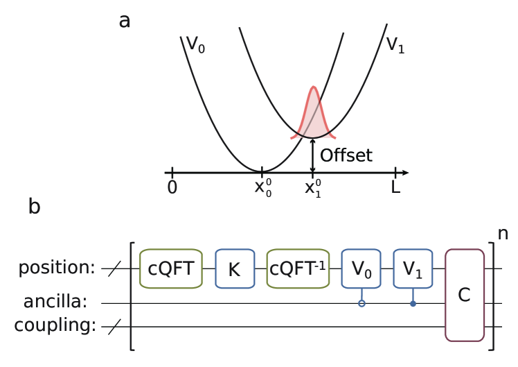
An ancilla qubit, , is entangled with the spacial register and controls the non-adiabatic dynamics accross the diabatic curves.
It is initialized in state () if the wavepacket at time is placed on the first (second) diabatic potential V0 (V1).
For concreteness we specialize to the Marcus model Marcus (1964, 1993) which provides a simplified description of the electron-transfer reaction rate driven by collective outer and inner sphere coordinates Siders and Marcus (1981).
In this model, the potentials of Eq. (1) are defined by . The two harmonic potentials of the diabatic curves differ by an energy shift , frequency , equilibrium position , and model the reactant and product states respectively.
We call offset the difference .
We use this setup in what follows and show its representation in Fig. 1a.
Resources scaling. The position is encoded in the qubit register as where is an integer which binary representation is encoded in the basis states of qubits.
Thus, in general, we require qubits to store the total wavefunction of the wavepacket in dimensions.
An ancillary register of size is needed to describe dynamics involving up to diabatic potential energy surfaces.
In the specific model considered here, we only need one ancillary qubit for the propagation of the wavepacket in and coupled through the non-adiabatic coupling operator .
Additionally, an extra qubit register is required to implement which size depends linearly on as well as on the shape of the coupling as explained later and in the Supplemental Material.
The time-evolution algorithm. The very first step of the dynamics resides in the initialization of the wavepacket in the quantum register. In the interest of clarity, this step will be discussed in further detail at the end of this Letter and in the Supplemental Material. Then the wavepacket is propagated under the action of the real-time evolution operator such that , using the Lie-Trotter-Suzuki product formulas Berry et al. (2007). A quantum circuit for implementing the time evolution under the kinetic operator and harmonic potentials was presented in Refs. Somma (2015); Benenti and Strini (2008) and is detailed in the Supplemental Material. The same logic can be extended to potentials described by a polynomial function of the position. Note that to account for negative values of the momentum, a shift of , where , is applied placing the zero momentum value at the center of the Brillouin zone. This choice implies the use of a centered Quantum Fourier Transform (cQFT) operator (see Supplemental Material for details) to implement the switch from the position to the momentum space. While the quantum circuit for the kinetic part of the evolution can directly be applied on the first qubits, the potential parts must be controlled by the state of the ancilla qubit, , such that the wavepacket evolves under the action of and when is in the and state respectively (here is the number of Trotter steps).
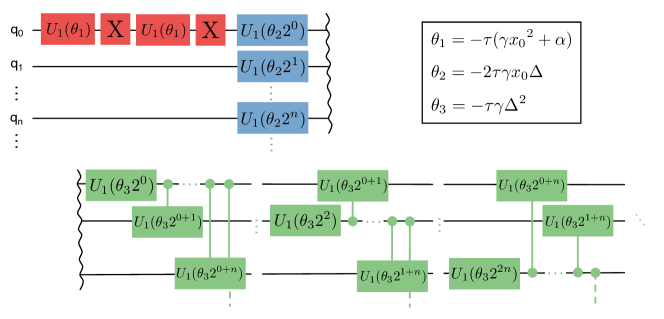
One of the main methodological novelties of this work resides in the encoding of the coupling operator which acts as
| (2) |
and thus corresponds to a rotation of the ancilla qubit around the axis by an angle .
The general approach consists in pre-computing a discretized function, , into additional qubits using quantum arithmetic.
While the number of gates and the number of additional qubits scale exponentially with the inverse desired accuracy for a general function Mitarai et al. (2019),
the resources can be kept reasonably low by approximating as a piecewise linear function Häner et al. (2018).
In the approach adopted here, the additional gates and ancilla qubits scale linearly with and with the number of pieces in the description of (see Supplemental Material and Refs. Woerner and Egger (2019); Stamatopoulos et al. (2019)).
Crucially, we observe that accurate results can be obtained by including only few pieces in .
A graphical representation of the quantum circuit used to encode the dynamics is shown in Fig. 1b.
Rates in the Marcus model. The model parameters are chosen to represent typical molecular dynamics Yonehara and Takatsuka (2010) and the simulation conditions were optimized to guarantee the convergence of the results (see the Supplemental Material). Therefore, we choose to discretize a space of length using 8 qubits and we select a time-step of 10 a.u.. The non-adiabatic coupling term, which in the reference model is a Gaussian function, is approximated with a step function giving the best trade-off between accuracy and number of additional qubits that, in this case, amounts to 9 qubits. The time evolution is performed for a total time of a.u. and repeated for different values of the offset between the two harmonic potential energy curves.
For the time being, we assume a Gaussian state preparation of the form (see below) Yonehara and Takatsuka (2010)
| (3) |
at the center of the potential curve at the right, , at (see Fig. 1a) with . The initial momentum is set to . This choice is motivated from the possibility to compare with the standard Marcus rate theory (see Supplemental Material). Note however that the qualitative behavior of the dynamics is not affected by the particular value of .
At each time step, the population fraction, , in the product well , is simply related to the expectation value of the ancilla qubit as (where is the Pauli operator ).
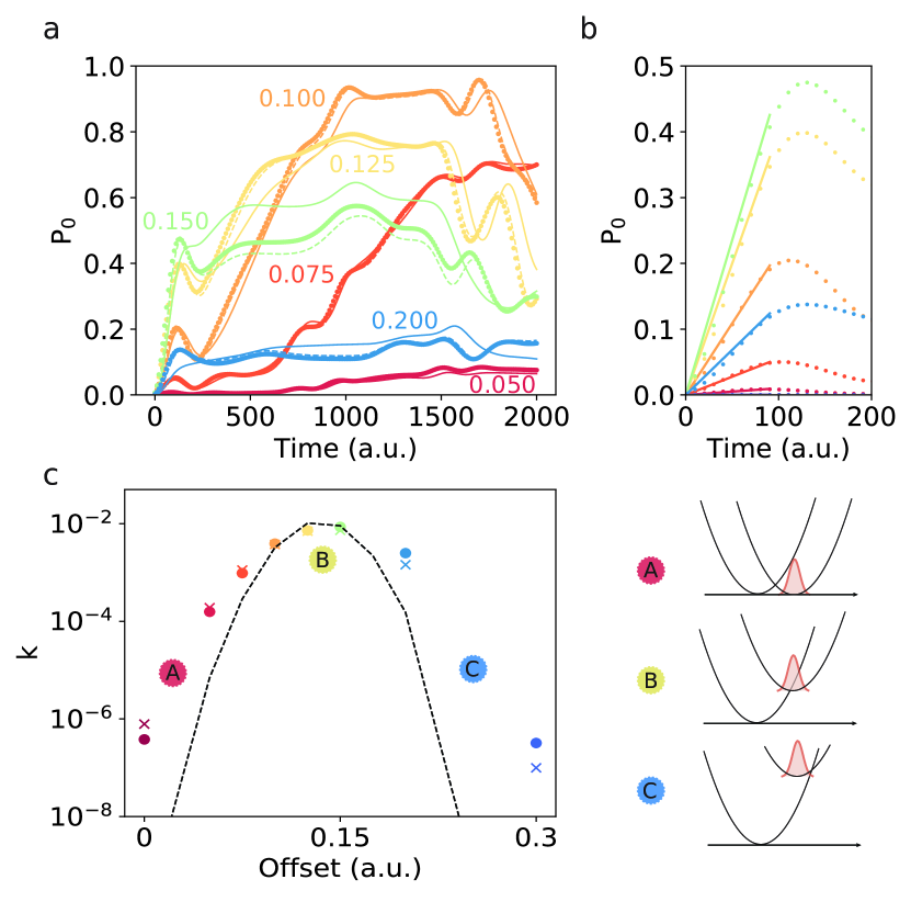
We run the dynamics for various offset values and show the time evolution of corresponding in Fig. 2a (dots), using a classical emulation of the corresponding quantum circuit.
The exact evolution obtained with the original, Gaussian, coupling (full lines) and with its piecewise approximation (dashed lines) is also reported demonstrating the correct implementation of the algorithm (the small discrepancies are due to Trotter errors).
Moreover, these results highlight that the piecewise linear approximation of the coupling function allows to recover the correct qualitative quantum dynamics.
Note that the accuracy of the results is controllable as it can be systematically increased by improving the representation of the coupling function, as well as by reducing the Trotter step.
We calculate the initial rate constant, , for each offset by taking the slope of the linear fit applied to the first ten steps of the dynamics as shown in Fig. 2b.
The rates obtained from the quantum dynamics (dots) and from the exact dynamics with the exact, Gaussian, coupling (crosses) are in good agreement and are summarized in Fig. 2c.
As expected, the population transfer rate increases with the offset in the normal Marcus regime, reaching a maximum value when the offset is equal to the reorganization energy before decreasing again in the inverted region,
thus recovering the expected volcano shape predicted by Marcus theory (dashed line in Fig. 2c).
Note that discrepancies between the Marcus rates, calculated for a carefully chosen effective temperature (see the Supplemental Material) and our rate estimates are expected, as we are performing a closed-system dynamics.
Initial state preparation.
To complete our presentation, we discuss an equally efficient initial state preparation method.
To this end, we rely on a more efficient Variational Quantum Eigensolver (VQE) Peruzzo et al. (2014); Yung et al. (2014); McClean et al. (2016); Wang et al. (2019) approach instead of quantum arithmetic based methods Grover and Rudolph (2002); Kitaev and Webb (2008).
As a proof of concept we show how to prepare a wavepacket defined as the ground state of the (arbitrarily chosen) Hamiltonian defined on a 3-qubit register (Supplemental Material for the detail).
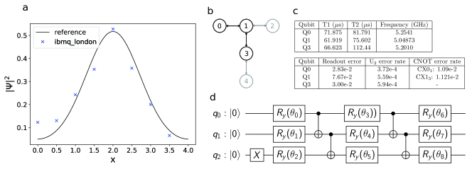
The parametrized circuit comprises three layers of rotations intersected of 2 layers of CNOT gates as shown in Fig. 3d.
In the Supplemental Material we study the convergence of the VQE in presence of noise with the state-of-the-art optimizer and show that it requires an important number of optimization steps as well as error mitigation.
Here the circuit can be optimized in a fully classical simulation of the VQE algorithm.
We employ this circuit on three qubits of the ibmq_london 5-qubit chip (see the hardware layout and the qubits specifications in Figs. 3b and 3c respectively).
Since in this example (i.e. the wavefunction is real) we simply display the modulo squared of the resulting wavefunction (obtained by measuring 8000 times in the position basis) in Fig. 3a. We also show the reference Gaussian function demonstrating the initialization of the desired wavepacket in the quantum computer.
Conclusion.
We introduced a quantum algorithm to simulate the propagation of a nuclear wavepacket across diabatic surfaces, featuring non-linear couplings.
The degrees of freedom are expressed in the first quantization formalism, as the position and momentum spaces are discretized and encoded in a position quantum register.
Ancilla registers are used to encode the real time evolution of the population transfer between the surfaces, and to realize the non-linear coupling operators.
The encoding of the problem is efficient in term of qubit resources, which scale logarithmically with the precision.
This impressive memory compression in storing the time-evolved wavefunction, represented in a systematically converging basis-set of a real space -point grid, readily realizes an exponential quantum advantage compared to classical algorithms.
As discussed, the proposed circuit to perform the coupled-time evolution only requires a polynomially scaling depth.
We demonstrate this approach to simulate the non-adiabatic dynamics of a wavepacket evolving in a Marcus model, consisting in two one-dimensional harmonic potentials shifted in energy by a variable offset.
This minimal model requires a feasible number of qubits (eighteen), so that the circuit can be classically emulated. The simulated dynamics are in excellent agreement with the exact propagation and we are able to observe the expected slowing down of the population transfer
in the so-called inverted region.
However, the circuit depth required to observe these dynamics greatly exceeds those currently feasible due to
the limited coherence time of present quantum hardware.
Therefore, we limit the hardware demonstration to the first part of the algorithm i.e. the Gaussian wavepacket initialization, on an IBM Q device.
As far as concerning the quantum resources (number of qubits), our algorithm can straightforwardly be extended to represent polynomial potential energy surfaces in -dimensions with a scaling .
Hence, a quantum computer with qubits would allow for the study of molecular systems characterized by up to 10 vibrational modes.
Reaching the limits of classical simulations Capano et al. (2014); Zhugayevych and Tretiak (2015), this approach will pave the way towards a better understanding of femto-chemistry processes, such as internal conversion and inter-system crossings, exciton formation and charge separation.
Acknowledgements. The authors thank Julien Gacon, Almudena Carrera Vazquez and Stefan Woerner for useful discussions and acknowledge financial support from the Swiss National Science Foundation (SNF) through the grant No. 200021-179312.
IBM, the IBM logo, and ibm.com are trademarks of International Business Machines Corp., registered in many jurisdictions worldwide. Other product and service names might be trademarks of IBM or other companies. The current list of IBM trademarks is available at https://www.ibm.com/legal/copytrade.
References
- Domcke and Stock (1997) W. Domcke and G. Stock, Advances in Chemical Physics 100, 1 (1997).
- Worth and Cederbaum (2004a) G. A. Worth and L. S. Cederbaum, Annual Review of Physical Chemistry 55, 127 (2004a).
- Domcke and Yarkony (2012) W. Domcke and D. R. Yarkony, Annual Review of Physical Chemistry 63, 325 (2012).
- Schuurman and Stolow (2018) M. S. Schuurman and A. Stolow, Annual Review of Physical Chemistry 69, 427 (2018).
- Yarkony (2001) D. R. Yarkony, The Journal of Physical Chemistry A 105, 6277 (2001).
- Hagfeldt and Graetzel (1995) A. Hagfeldt and M. Graetzel, Chemical Reviews 95, 49 (1995).
- Tang and Vanslyke (1987) C. W. Tang and S. A. Vanslyke, Applied Physics Letters 51, 913 (1987).
- Bersuker (2013) I. Bersuker, The Jahn-Teller effect and vibronic interactions in modern chemistry (Springer Science & Business Media, 2013).
- Nelson et al. (2020) T. Nelson, A. White, J. Bjorgaard, A. Sifain, Y. Zhang, B. Nebgen, S. Fernandez-Alberti, D. Mozyrsky, A. Roitberg, and S. Tretiak, Chemical Reviews 120 (2020), 10.1021/acs.chemrev.9b00447.
- Tavernelli (2015) I. Tavernelli, Accounts of Chemical Research 48, 792 (2015).
- Jang and Mennucci (2018) S. J. Jang and B. Mennucci, Rev. Mod. Phys. 90, 035003 (2018).
- Worth and Cederbaum (2004b) G. A. Worth and L. S. Cederbaum, Annual Review of Physical Chemistry 55, 127 (2004b).
- Zener (1932) C. Zener, Proc. R. Soc. A 137, 696 (1932).
- Miller (1970) W. H. Miller, J. Chem. Phys 53, 3578 (1970).
- Ehrenfest (1927) P. Ehrenfest, Zeitschrift für Physik 45, 455 (1927).
- Tully (1990) J. C. Tully, The Journal of Chemical Physics 93, 1061 (1990).
- Curchod and Martínez (2018) B. F. E. Curchod and T. J. Martínez, Chemical Reviews 118, 3305 (2018).
- Sun and Miller (1997) X. Sun and W. H. Miller, The Journal of Chemical Physics 106, 6346 (1997).
- Kosloff (1994) R. Kosloff, Annual Review of Physical Chemistry 45, 145 (1994).
- Garraway and Suominen (1995) B. M. Garraway and K.-A. Suominen, Reports on Progress in Physics 58, 365 (1995).
- Huang et al. (2018) J. Huang, S. Liu, D. H. Zhang, and R. V. Krems, Physical Review Letters 120, 143401 (2018).
- Meyer et al. (1990) H.-D. Meyer, U. Manthe, and L. S. Cederbaum, Chemical Physics Letters 165, 73 (1990).
- Beck et al. (2000) M. H. Beck, A. Jäckle, G. A. Worth, and H.-D. Meyer, Physics Reports 324, 1 (2000).
- Egorova et al. (2001) D. Egorova, A. Kühl, and W. Domcke, Chemical Physics 268, 105 (2001).
- Meyer and Worth (2003) H.-D. Meyer and G. A. Worth, Theoretical Chemistry Accounts 109, 251 (2003).
- Burghardt et al. (2008) I. Burghardt, K. Giri, and Worth, J. Chem. Phys. 129, 174104 (2008).
- Martinazzo et al. (2006) R. Martinazzo, M. Nest, P. Saalfrank, and G. F. Tantardini, J. Chem. Phys. 125, 194102 (2006).
- Martínez and Levine (1997) T. J. Martínez and R. D. Levine, Journal of the Chemical Society, Faraday Transactions 93, 941 (1997).
- Feynman (1999) R. P. Feynman, International Journal of Theoretical Physics 21 (1999).
- Kandala et al. (2017) A. Kandala, A. Mezzacapo, K. Temme, M. Takita, M. Brink, J. M. Chow, and J. M. Gambetta, Nature 549, 242 (2017).
- Colless et al. (2018) J. I. Colless, V. V. Ramasesh, D. Dahlen, M. S. Blok, M. Kimchi-Schwartz, J. McClean, J. Carter, W. De Jong, and I. Siddiqi, Physical Review X 8, 011021 (2018).
- Kandala et al. (2019) A. Kandala, K. Temme, A. D. Córcoles, A. Mezzacapo, J. M. Chow, and J. M. Gambetta, Nature 567, 491 (2019).
- Nam et al. (2019) Y. Nam, J.-S. Chen, N. C. Pisenti, K. Wright, C. Delaney, D. Maslov, K. R. Brown, S. Allen, J. M. Amini, J. Apisdorf, et al., arXiv preprint arXiv:1902.10171 (2019).
- Ollitrault et al. (2019) P. J. Ollitrault, A. Kandala, C.-F. Chen, P. K. Barkoutsos, A. Mezzacapo, M. Pistoia, S. Sheldon, S. Woerner, J. Gambetta, and I. Tavernelli, arXiv preprint arXiv:1910.12890 (2019).
- Zalka (1998) C. Zalka, Proceedings of the Royal Society of London. Series A: Mathematical, Physical and Engineering Sciences 454, 313 (1998).
- Wiesner (1996) S. Wiesner, arXiv preprint arXiv:quant-ph/9603028 (1996).
- Kassal et al. (2008) I. Kassal, S. P. Jordan, P. J. Love, M. Mohseni, and A. Aspuru-Guzik, Proceedings of the National Academy of Sciences 105, 18681 (2008).
- Benenti and Strini (2008) G. Benenti and G. Strini, American Journal of Physics 76, 657 (2008).
- Somma (2015) R. D. Somma, arXiv preprint arXiv:1503.06319v2 (2015).
- Macridin et al. (2018) A. Macridin, P. Spentzouris, J. Amundson, and R. Harnik, Physical Review Letters 121, 110504 (2018).
- Ballester et al. (2012) D. Ballester, G. Romero, J. J. García-Ripoll, F. Deppe, and E. Solano, Physical Review X 2, 021007 (2012).
- Leppäkangas et al. (2018) J. Leppäkangas, J. Braumüller, M. Hauck, J.-M. Reiner, I. Schwenk, S. Zanker, L. Fritz, A. V. Ustinov, M. Weides, and M. Marthaler, Physical Review A 97, 052321 (2018).
- Marcus (1993) R. A. Marcus, Reviews of Modern Physics 65, 599 (1993).
- Marcus (1964) R. A. Marcus, Annual Review of Physical Chemistry 15, 155 (1964).
- Siders and Marcus (1981) P. Siders and R. A. Marcus, Journal of the American Chemical Society 103, 748 (1981).
- Berry et al. (2007) D. W. Berry, G. Ahokas, R. Cleve, and B. C. Sanders, Communications in Mathematical Physics 270, 359 (2007).
- Mitarai et al. (2019) K. Mitarai, M. Kitagawa, and K. Fujii, Physical Review A 99, 012301 (2019).
- Häner et al. (2018) T. Häner, M. Roetteler, and K. M. Svore, arXiv preprint arXiv:1805.12445 (2018).
- Woerner and Egger (2019) S. Woerner and D. J. Egger, npj Quantum Information 5, 1 (2019).
- Stamatopoulos et al. (2019) N. Stamatopoulos, D. J. Egger, Y. Sun, C. Zoufal, R. Iten, N. Shen, and S. Woerner, arXiv preprint arXiv:1905.02666 (2019).
- Yonehara and Takatsuka (2010) T. Yonehara and K. Takatsuka, The Journal of Chemical Physics 132, 244102 (2010).
- Peruzzo et al. (2014) A. Peruzzo, J. McClean, P. Shadbolt, M.-H. Yung, X.-Q. Zhou, P. J. Love, A. Aspuru-Guzik, and J. L. O’Brien, Nature Communications 5 (2014).
- Yung et al. (2014) M.-H. Yung, J. Casanova, A. Mezzacapo, J. Mcclean, L. Lamata, A. Aspuru-Guzik, and E. Solano, Scientific Reports 4, 3589 (2014).
- McClean et al. (2016) J. R. McClean, J. Romero, R. Babbush, and A. Aspuru-Guzik, New Journal of Physics 18, 023023 (2016).
- Wang et al. (2019) D. Wang, O. Higgott, and S. Brierley, Physical Review Letters 122, 140504 (2019).
- Grover and Rudolph (2002) L. Grover and T. Rudolph, arXiv preprint quant-ph/0208112 (2002).
- Kitaev and Webb (2008) A. Kitaev and W. A. Webb, arXiv preprint arXiv:0801.0342 (2008).
- Capano et al. (2014) G. Capano, M. Chergui, U. Rothlisberger, I. Tavernelli, and T. J. Penfold, The Journal of Physical Chemistry A 118, 9861 (2014).
- Zhugayevych and Tretiak (2015) A. Zhugayevych and S. Tretiak, Annual Review of Physical Chemistry 66, 305 (2015).
Supplementary Information for: Non-adiabatic molecular quantum dynamics with quantum computers
I Lie-Trotter decomposition
The wavepacket is propagated under the action of the real-time evolution operator as
| (S1) |
In practice the evolution operator is decomposed using Lie-Trotter-Suzuki product formulas Berry et al. (2007) to reduce the error arising from the fact that the kinetic part, , of the Hamiltonian (acting in the momentum space) does not commute with the potential, , and coupling, , terms (in the position space). In this work we use the basic Lie-Trotter formula. Hence the evolution operator becomes
| (S2) |
II Centered Quantum Fourier Transform
The minimum of the momentum space is placed at the center of the Brillouin zone by applying a shift, , to allow the momentum to take negative values. This must be taken into account in the QFT. In the case where the momentum space in centered exactly around the middle of the array we can simply add a X gate on the last qubit right before and after the QFT and QFT-1 operations such that they undergo a cyclic permutation:
| (S3) |
III Quantum circuit for quadratic curve
The circuit for implementing any operator, , of quadratic shape, i.e. which matrix elements are defined by
| (S4) |
is discussed in Benenti and Strini (2008) and depicted in Fig. S1. The number of gates scales as with the number of qubits.
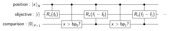
IV Evaluation of a piecewise linear function
The piecewise linear function is defined as:
| (S5) |
where is total the number of pieces in the function. A rotation of the type can be applied on an objective qubit, , in a similar way as presented in the previous section, by discretizing the variable as in the states of qubits (called position qubits). The pieces of the function are delimited by breakpoints. The circuit for implementing the full operator also requires additional comparison qubits which role is clarified below. The number of comparison qubits is while the number of gates scales as Stamatopoulos et al. (2019). The algorithm works as follows.
-
1.
Apply R to .
-
2.
Apply CR to controlled by for each qubit in the position register.
-
3.
Check if break point using the comparison qubits and encode this information in the state of one comparison qubit .
-
4.
Apply CR to controlled by .
-
5.
Apply CR to controlled by for each qubit in the position register as well as by .
-
6.
Repeat step 3, 4 and 5 for each piece of replacing the and indexes by and respectively.
For clarity we also display the corresponding circuit in Fig. S2.
V Parameters setting
This section is devoted to a preliminary study of the coupling shape, the space discretization and the Trotter error in order to extract reasonable parameters for the quantum evolution of the wavepacket. The non-adiabatic model Yonehara and Takatsuka (2010) employed in this work comprises two harmonic potential functions described by and with , and . The coupling potential is given by with . The reduced mass is 1818.18 a.u. The length, , of the box is fixed to 20. The wavefunction is initialized to a full quantum wavepacket,
| (S6) |
with , and .
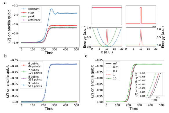
First, we approximate the coupling shape with a piecewise linear function of the position. We try different coupling shapes shown on the right side of Fig. S3a: a constant coupling (one piece), a step (three pieces) and a peak (four pieces). The breaking points of the step and peak shapes are chosen to preserve the area under the reference curve given by
| (S7) |
The reference coupling shape is shown together with the two potential energy curves on the lower left panel. The initial wavepacket is propagated with the exact time evolution (no Trotter error) and the various coupling shapes. The number of qubit for the discretization of the position and momentum space is fixed to 9. The expectation value of the ancilla qubit measured in the Z basis is displayed in Fig. S3a (left) and show both the step and peek coupling shapes provide qualitatively correct results. Although the peak shaped coupling leads to more accurate results, we choose to work with the step shape as it allows to save one qubit while remaining in good accuracy.
As a second step, we evolve (using state-vector simulations) the wavepacket with the reference coupling shape and vary the number of qubits in the quantum register (and therefore the size of the grid’s spacing). For the system under study, we find that a minimum of 8 qubits, equivalent to 256 grid points, is needed to reproduce faithfully the desired dynamics (see Fig. S3b).
Finally we monitor the Trotter error. To do so, the number of qubits is kept fixed to 8, while the time step is varied. In Fig. S3c, we show that qualitatively correct results can be obtained with a time step as large as 10 a.u., value that we chose for the production runs.
VI Initialization of the wavepacket
The initial wavepacket is prepared in the quantum computer by applying the corresponding quantum circuit. This quantum circuit can be found with the VQE algorithm Peruzzo et al. (2014); Yung et al. (2014); McClean et al. (2016); Wang et al. (2019). At each iteration of the VQE, the energy, , of the trial wavefunction is calculated in the following way,
| (S8) | |||
| (S9) |
and
| (S10) |
where and are the potential and kinetic energy respectively. is the total number of measurements done on the quantum computer to obtain the statistics, per basis. (with , ) is the number of measurement that collapsed onto the qubit basis state corresponding to the binary representation of integer . For the potential energy term the counts are obtained by measuring in the position basis where measurements can straightly be applied whereas the kinetic term requires applying a QFT beforehand to ensure that measurements are done in the momentum basis.
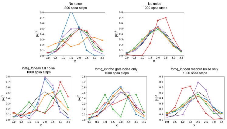
We tested the ability of preparing the desired wavepacket with VQE for a 3-qubit system. In this example the wavepacket is described as the ground state of the Hamiltonian . The size of the box is . The trial wavefunction Ansatz is shown in Fig. 3d of the main text. At the beginning of the VQE, the quantum state is initialized as a (discrete) Dirac delta function , namely the bit string . We run the VQE algorithm classically in a quantum simulator where the quantum measurements are simulated by projecting the statevector on the basis states 8000 times. Moreover, a noise model can be added to the classical simulator in order to simulate the gate noise (depolarization and thermal relaxation) and readout error characteristic of the available quantum computers. In what follows we employ a noise model based on the properties of the ibm_q_london 5-qubit device. The layout and the properties of the exploited qubits are given in Fig. 3b and c of the main text. We use the state-of-the-art optimizer for noisy optimization problems namely the Simultaneous Perturbation Stochastic Approximation (SPSA)Spall (2000). We run five different experiments. Because the optimization process is stochastic, each experiment is composed of five VQE simulations. The results are displayed in Fig. S4. In the first two experiments we completely turn off the noise model to study the bare convergence of the optimization. In the first case, the VQEs are stopped after 200 SPSA steps while in the second they are ended at 1000 steps. In the first case none of the VQEs converge whereas in the second case four out of five did showing that even for a circuit as shallow as the one employed for this task (3 qubits, 9 variational parameters and 4 CNOT gates) the convergence of the SPSA algorithm requires a consequent number of iterations. We then turn on the noise model fully. In this case, none of the VQEs are able to recover the desired Gaussian shape after 1000 SPSA steps leading to the conclusion that error mitigation is imperative. Finally we realize two experiments by keeping only 1. the gate noise and 2. the readout errors. In both cases three out of five VQEs were able to reasonably approach the desired shape showing that by reducing the noise (e.g. with error mitigation) the SPSA optimizer may be robust enough to approximate the ground state within reasonable accuracy.
VII Marcus rates
The Marcus rate constants used in the main text are given by Marcus (1956); Nitzan (2006)
| (S11) |
where is the electronic coupling, the reorganization energy, the offset and the Planck’s constant and the reciprocal of Boltzmann’s constant, , times the temperature .
Seeking for a qualitative comparison between the rates resulting from the quantum dynamics and the Marcus rates we need to determine a sensible value to insert in this equation. Since our quantum dynamics does not include dissipation or any coupling with the environment, the temperature is not present as an explicit parameter in our setting. The route we adopt here is to extract an effective temperature by a careful initialization of the wavepacket.
To do so, we look for an initial position and momentum, and , for which the density of states given by the initial Gaussian wavepacket, , can be described by a Boltzmann distribution such that
| (S12) |
where are the eigenstates of the harmonic oscillator defined by and is the energy of state . We choose , the center of and calculate the for several values of . We then fit the resulting distribution to a Boltzmann distribution to extract a value for (see Fig. S5).
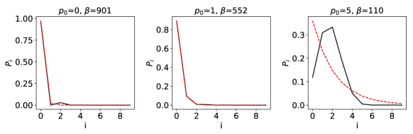
We find that for a value of the density of states can be well represented by a Boltzmann distribution defined by . This set our choice for the parameter in our simulations and for the parameter in the Marcus rate theory to compare with. We notice obviously that the quantum dynamics can be performed with any choice of , but this specific choice is made to enable a qualitative comparison with Marcus theory. Therefore, we run the quantum dynamics initializing the Gaussian wavepacket with and and compute the Marcus rates with .
References
- Berry et al. (2007) D. W. Berry, G. Ahokas, R. Cleve, and B. C. Sanders, Communications in Mathematical Physics 270, 359 (2007).
- Benenti and Strini (2008) G. Benenti and G. Strini, American Journal of Physics 76, 657 (2008).
- Stamatopoulos et al. (2019) N. Stamatopoulos, D. J. Egger, Y. Sun, C. Zoufal, R. Iten, N. Shen, and S. Woerner, arXiv preprint arXiv:1905.02666 (2019).
- Yonehara and Takatsuka (2010) T. Yonehara and K. Takatsuka, The Journal of Chemical Physics 132, 244102 (2010).
- Peruzzo et al. (2014) A. Peruzzo, J. McClean, P. Shadbolt, M.-H. Yung, X.-Q. Zhou, P. J. Love, A. Aspuru-Guzik, and J. L. O’Brien, Nature Communications 5 (2014).
- Yung et al. (2014) M.-H. Yung, J. Casanova, A. Mezzacapo, J. Mcclean, L. Lamata, A. Aspuru-Guzik, and E. Solano, Scientific Reports 4, 3589 (2014).
- McClean et al. (2016) J. R. McClean, J. Romero, R. Babbush, and A. Aspuru-Guzik, New Journal of Physics 18, 023023 (2016).
- Wang et al. (2019) D. Wang, O. Higgott, and S. Brierley, Physical Review Letters 122, 140504 (2019).
- Spall (2000) J. C. Spall, IEEE Transactions on Automatic Control 45, 1839 (2000).
- Marcus (1956) R. A. Marcus, The Journal of chemical physics 24, 966 (1956).
- Nitzan (2006) A. Nitzan, Chemical dynamics in condensed phases: relaxation, transfer and reactions in condensed molecular systems (Oxford university press, 2006).