Density Deconvolution with Normalizing Flows

Abstract

Density deconvolution is the task of estimating a probability density function given only noise-corrupted samples. We can fit a Gaussian mixture model to the underlying density by maximum likelihood if the noise is normally distributed, but would like to exploit the superior density estimation performance of normalizing flows and allow for arbitrary noise distributions. Since both adjustments lead to an intractable likelihood, we resort to amortized variational inference. We demonstrate some problems involved in this approach, however, experiments on real data demonstrate that flows can already out-perform Gaussian mixtures for density deconvolution.

1 Introduction

Density estimation is the fundamental statistical task of estimating the density of a distribution given a finite set of measurements. However, in many scientific fields (see examples in Carroll et al., 2006), one only has access to a noise-corrupted set of measurements. Given knowledge of the statistics of the noise, density deconvolution methods attempt to recover the density function of the unobserved noise-free samples rather than the noisy measurements.

In this work we consider the problem of additive noise, where observed samples $\{{\mathbf{w}}_{i}\}_{i=1}^{m}$ are produced by adding independent noise to unobserved values $\{{\mathbf{v}}_{i}\}_{i=1}^{m}$,

$${\mathbf{w}}_{i}={\mathbf{v}}_{i}+{\mathbf{n}}_{i}.$$ (1)

We also assume that the density function of the noise $p_{{\mathbf{n}}_{i}}\kern-1.0pt({\mathbf{n}}_{i})$ is perfectly known for every observation. The density function of observations ${\mathbf{w}}_{i}$ is then a convolution

$$p({\mathbf{w}}_{i})=\int_{\mathbf{v}}p_{{\mathbf{n}}_{i}}\kern-1.0pt({\mathbf{w}}_{i}-{\mathbf{v}})\,p({\mathbf{v}})\,d{\mathbf{v}}.$$ (2)

When the noise distribution is constant, we could estimate the density of the observations ${\mathbf{w}}$ with any density estimator and then solve Equation 2, e.g. with a kernel density estimator using Fourier transforms (e.g., Liu & Taylor, 1989; Carroll & Hall, 1988; Fan, 1991; Devroye, 1989) or wavelet decompositions (Pensky & Vidakovic, 1999).

When the noise distribution is different for each observation, we only have one sample from each convolved density. This extreme deconvolution setting (Bovy et al., 2011) has previously been tackled by fitting a Gaussian Mixture Model (GMM) to the underlying density $p({\mathbf{v}})$. When the noise distributions are all Gaussian, the marginal likelihood $p({\mathbf{w}}_{i})$ is tractable, and the GMM can be fitted by Expectation-Maximisation (EM, Bovy et al., 2011) or Stochastic Gradient Descent (SGD, Ritchie & Murray, 2019).

Given enough mixture components, any density function can be approximated arbitrarily closely using GMMs. In practice, however, other representations of densities can be easier to fit, and often generalize better. There is growing interest in normalizing flows (Tabak & Vanden-Eijnden, 2010; Tabak & Turner, 2013), a class of methods that transform a simple source density into a complex target density. Normalizing flows are an efficient alternative to GMMs (e.g., Rezende & Mohamed, 2015), providing both good scalability and high expressivity, and have shown promise in applications similar to density deconvolution (Cranmer et al., 2019).

In this work, we model the underlying density $p({\mathbf{v}})$ with a normalizing flow. The marginal likelihood $p({\mathbf{w}}_{i})$ is intractable, so we resort to approximate inference. We use amortized variational inference (Section 2), closely following Variational Auto-Encoders (VAEs, Kingma & Welling, 2014; Rezende et al., 2014). Unlike for VAEs, in our framework, the model between the latent ${\mathbf{v}}$ and observed ${\mathbf{w}}$ vectors is fixed.

In this proof of concept, we use a fixed Gaussian noise distribution, but our approach would also allow us to use arbitrary and varying noise distributions, as found in realistic applications (e.g., Anderson et al., 2018). In a setting well-suited to the existing Gaussian mixture approach, we find that fitting flows is harder (Section 4.1), possibly motivating further work on approximate inference in this setting. Nevertheless, on real data, we demonstrate that flows can already outperform GMMs for density deconvolution (Section 4.2).

2 Methods

We take a variational approach (Jordan et al., 1999) to density deconvolution. Introducing an approximate posterior $q_{\bm{\phi}}({\mathbf{v}})$ gives a lower bound to the log-marginal likelihood

$$\log p({\mathbf{w}}_{i})=\log\int_{\mathbf{v}}p_{{\mathbf{n}}_{i}}\kern-1.0pt({\mathbf{w}}_{i}\!-\!{\mathbf{v}})\,p_{\bm{\theta}}({\mathbf{v}})\,d{\mathbf{v}}$$ (3)

$$=\log\int_{\mathbf{v}}p_{{\mathbf{n}}_{i}}\kern-1.0pt({\mathbf{w}}_{i}\!-\!{\mathbf{v}})\,p_{\bm{\theta}}({\mathbf{v}})\,\frac{q_{\bm{\phi}}({\mathbf{v}})}{q_{\bm{\phi}}({\mathbf{v}})}\,d{\mathbf{v}}$$ (4)

$$\geq\mathbb{E}_{q}[\log p_{{\mathbf{n}}_{i}}\kern-1.0pt({\mathbf{w}}_{i}\!-\!{\mathbf{v}})]-\mathsf{D}_{\mathrm{KL}}(q_{\bm{\phi}}({\mathbf{v}})\,\|\,p_{\bm{\theta}}({\mathbf{v}}))={\mathcal{L}},$$ (5)

where ${\mathcal{L}}$ is the evidence lower bound (ELBO, see Appendix A). Our approximate posterior $q_{\bm{\phi}}({\mathbf{v}})$, a recognition network, represents beliefs about an underlying value ${\mathbf{v}}$ given an observation ${\mathbf{w}}$ and the parameters of the noise.

The ELBO gives a unified objective for both the parameters ${\bm{\theta}}$ of the model and the parameters ${\bm{\phi}}$ of the recognition network. Stochastic gradient descent only needs unbiased estimates of the ELBO, which we obtain by Monte Carlo

$${\mathcal{L}}\approx{\mathcal{L}}(K)=\frac{1}{K}\sum_{k=1}^{K}\log\left[\frac{p_{{\mathbf{n}}_{i}}\kern-1.0pt({\mathbf{w}}_{i}-{\mathbf{v}}_{k})\,p_{\bm{\theta}}({\mathbf{v}}_{k})}{q_{\bm{\phi}}({\mathbf{v}}_{k})}\right],$$ (6)

where $K$ Monte Carlo samples are simulated ${\mathbf{v}}_{k}\sim q_{\bm{\phi}}({\mathbf{v}})$.

Our variational approach follows that of Variational Auto-Encoders (VAEs, Kingma & Welling, 2014; Rezende et al., 2014), which provide a framework for amortized variational inference in graphical models. The focus of VAEs, however, is usually to build generative models matching the observations ${\mathbf{w}}$. In contrast, our main target is estimating an underlying density function $p({\mathbf{v}})$. For certain applications, e.g. denoising a noisy measurement, we may also be interested in the approximate posterior $q_{{\bm{\phi}}}({\mathbf{v}})$. Another difference between our method and VAEs is that we do not learn a likelihood model between the latent variables ${\mathbf{v}}$ and the observations ${\mathbf{w}}$. Instead, our “likelihood model” is fully-characterized by the problem itself as $p_{{\mathbf{n}}_{i}}\kern-1.0pt({\mathbf{w}}_{i}-{\mathbf{v}})$.

We model both $p_{\bm{\theta}}({\mathbf{v}})$ and $q_{\bm{\phi}}({\mathbf{v}})$ as normalizing flows. Normalizing flows model probability density functions by transforming a source density $\pi({\mathbf{u}})$ into a target density $\hat{\pi}({\mathbf{v}})$ using an invertible, differentiable transformation $\mathsf{T}$

$${\mathbf{v}}=\mathsf{T}({\mathbf{u}}).$$ (7)

The density of ${\mathbf{v}}$ can be computed using the change-of-variable formula

$$\hat{\pi}({\mathbf{v}})=\frac{\pi\left(\mathsf{T}^{-1}({\mathbf{v}})\right)}{\absolutevalue{\det\frac{\partial\mathsf{T}}{\partial{\mathbf{u}}}\left(\mathsf{T}^{-1}({\mathbf{v}})\right)}}$$ (8)

In particular, we model $p_{\bm{\theta}}({\mathbf{v}})$ and $q_{\bm{\phi}}({\mathbf{v}})$ with autoregressive flows. For $p_{\bm{\theta}}({\mathbf{v}})$ we use a Masked Autoregressive Flow (MAF, Papamakarios et al., 2017), where a single neural network pass can compute $\mathsf{T}^{-1}({\mathbf{v}})$, and therefore the densities $\hat{\pi}({\mathbf{v}})$ required during training. Inverting the network, to generate samples, requires $D$ neural network passes for $D$-dimensional data. For $q_{\bm{\phi}}({\mathbf{v}})$ we use the same network architecture to represent $\mathsf{T}({\mathbf{u}})$, corresponding to an Inverse Autoregressive Flow (IAF, Kingma et al., 2016). During training, this choice gives fast one-pass generation of samples with their densities. For an extensive review on normalizing flows, we refer the reader to Papamakarios et al. (2019).

3 Related Work

Importance weighting: The Importance Weighted Autoencoder (Burda et al., 2015) has the same architecture as the standard VAE, however, it is trained on a lower bound that is tighter than the standard ELBO. Applying this idea to our model results in the following lower bound:

$$\log p({\mathbf{w}}_{i}) \geq\log\left[\frac{1}{K}\sum_{k=1}^{K}\frac{p_{{\mathbf{n}}_{i}}\kern-1.0pt({\mathbf{w}}_{i}-{\mathbf{v}}_{k})\,p_{\bm{\theta}}({\mathbf{v}}_{k})}{q_{\bm{\phi}}({\mathbf{v}}_{k})}\right]$$ (9)

$$={\mathcal{L}}_{\rm{IW}}(K).$$ (10)

It can be shown (Cremer et al., 2017) that, in expectation, ${\mathcal{L}}_{\rm{IW}}(K)$ is equivalent to ${\mathcal{L}}(K)$ with an implicit, more expressive approximate posterior. A theoretical advantage of ${\mathcal{L}}_{\rm{IW}}(K)$ over ${\mathcal{L}}(K)$ is that the former is consistent (under some mild boundedness assumptions, Burda et al., 2015, Theorem 1), i.e., $\lim_{K\to\infty}{\mathcal{L}}_{\rm{IW}}(K)=\log p({\mathbf{w}}_{i})$.

In fact, it is possible to construct an unbiased estimator of $\log p({\mathbf{w}}_{i})$ using ${\mathcal{L}}_{\rm{IW}}(K)$ with finite $K$ (Luo et al., 2020), in combination with a Russian Roulette Estimator (Kahn, 1955). A drawback of this approach is that there is no guarantee that the variance of the estimator is finite.

Inference suboptimality: When using the ELBO, or ${\mathcal{L}}_{\rm{IW}}(K)$ with finite $K$, we only have a bound on the marginal log-likelihood $\log p({\mathbf{w}}_{i})$. This bound is loose when the approximate posterior is incorrect, which happens either because the form of the posterior cannot be represented, or because the recognition network does not produce good variational parameters for all data points. Both issues can be overcome by choosing the approximate posterior from an expressive variational family  (Cremer et al., 2018), which is why we use a flow.

Expressive priors for representation learning: The standard VAE has a fixed prior, usually a multivariate standard normal distribution, but VAEs with more expressive priors have been proposed. Expressive priors are particularly useful when the distribution of the latent variables is used for representation learning.

A simple generalization for the prior is a learnable GMM (e.g Nalisnick et al., 2016; Dilokthanakul et al., 2016), which in our context would result in the existing extreme deconvolution model (Bovy et al., 2011), with no need for variational inference. Another approach is to model the prior with a collection of categorical distributions (e.g. van den Oord et al., 2017), which would be appropriate if an observation is well-modeled as a composition of prototype sources. We use MAF, because for the applications we have in mind (e.g., Anderson et al., 2018), we want to use a flexible, continuous prior representation. VAEs have also used autoregressive flow priors before (Chen et al., 2017).

4 Experiments

In this section, we compare our method to a baseline of GMMs fitted with the Extreme Deconvolution (XD) model (Bovy et al., 2011), as by Ritchie & Murray (2019).

4.1 Mixture of Gaussians

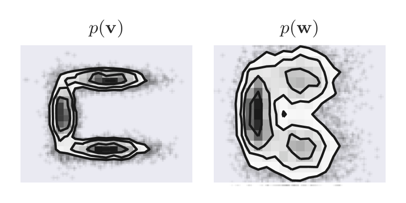
In this synthetic task, the target underlying density is a mixture of Gaussians. We fit the models from observations that include additional noise from a Gaussian with fixed covariance. Figure 1 shows density plots of both the latent data ${\mathbf{v}}$ and the observed data ${\mathbf{w}}$.

The exact posterior for a latent datapoint given a noisy observation is itself a mixture of Gaussians, and for some observations the components may be highly isolated. We have deliberately picked an example where the prior $p({\mathbf{v}})$ should be reasonably easy for a flow to model, but the posterior $p({\mathbf{v}}\,|\,{\mathbf{w}})$ may cause issues for flows, as they are known to have trouble fitting mixture of Gaussians when the components are well-separated (e.g., Jaini et al., 2019). Full experimental details are reported in Appendix B.1

Table 1 reports test average negative log-likelihood on both ${\mathbf{v}}$ and ${\mathbf{w}}$, referred to as $\log p({\mathbf{v}})$ and $\log p({\mathbf{w}})$, respectively. We estimate $\log p({\mathbf{w}})$ using ${\mathcal{L}}_{\rm{IW}}(100)$. The GMM, the true model class, has the best results for both ${\mathbf{v}}$ and ${\mathbf{w}}$. The flows give quite close estimates for $\log p({\mathbf{w}})$ when $K>1$ for both ${\mathcal{L}}$ and ${\mathcal{L}}_{\rm{IW}}$, but show very high variance in their estimates of $\log p({\mathbf{v}})$ relative to the variance for $\log p({\mathbf{w}})$.

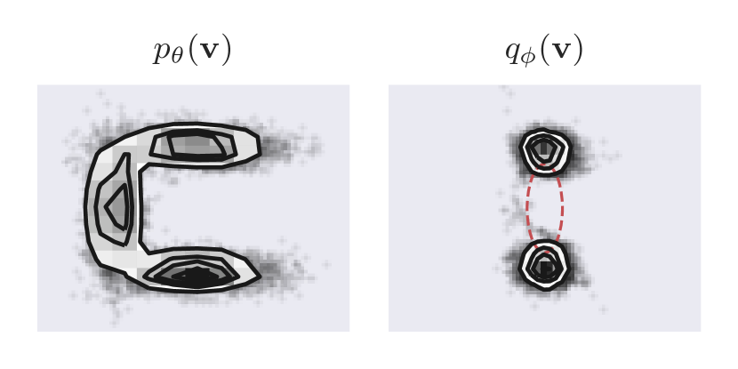
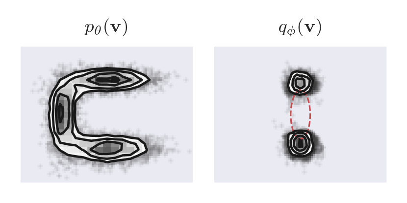
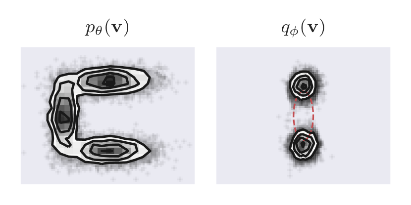
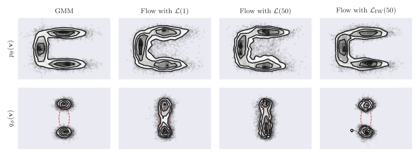
The top row of Figure 2 shows example density plots using samples from the priors of our fitted models. The fitted GMM has matched the ground truth GMM closely. The flows recover the broad shape of the ground truth model, but those trained with ${\mathcal{L}}(1)$ and ${\mathcal{L}}(50)$ put too much mass in the centre. The flow trained with ${\mathcal{L}}_{\rm{IW}}(50)$ matched the Gaussian mixture model on the run shown, but the results had high variance, and other runs do not look as good.

The bottom row of Figure 2 shows example posteriors for the fitted models. The exact posterior for the GMM has two isolated modes, and is a close match to the ground truth posterior. The approximate posteriors for the flows trained with ${\mathcal{L}}(1)$ and ${\mathcal{L}}(50)$ are not good matches to the GMM posterior, as neither have isolated modes, but are reasonably consistent with their corresponding priors. The approximate posterior for the flow trained with ${\mathcal{L}}_{\rm{IW}}(50)$ uses samples drawn from $q_{{\bm{\phi}}}$ with sampling-importance-resampling (e.g., Rubin, 1988). The resampling reflects this recognition network’s role as an adaptive proposal distribution under the ${\mathcal{L}}_{\rm{IW}}$ objective rather than a direct approximation to the posterior (Cremer et al., 2017). This reweighted approximation is a much better match to the ground truth posterior, but as with the prior, the variance across training runs was high, and other examples are qualitatively worse.

Figure 1: 2D histograms of training data for synthetic experiments. Contour lines are estimated 0.5/1/1.5/2-$\sigma$ levels, with samples in the tails plotted directly. Left: Latent data sampled from a mixture of Gaussians. Right: Observed data created by adding noise to samples from $p({\mathbf{v}})$.

Method	K	$-\log p({\mathbf{v}})$	$-\log p({\mathbf{w}})$
XD-GMM	–	$2.667\pm 0.000$	$3.600\pm 0.000$
Flow (${\mathcal{L}}$)	1	$2.897\pm 0.046$	$3.609\pm 0.002$
	10	$3.015\pm 0.228$	$3.607\pm 0.002$
	25	$2.858\pm 0.077$	$3.606\pm 0.004$
	50	$2.913\pm 0.174$	$3.605\pm 0.001$
Flow (${\mathcal{L}}_{\rm{IW}}$)	10	$2.854\pm 0.083$	$3.604\pm 0.002$
	25	$2.871\pm 0.045$	$3.604\pm 0.001$
	50	$3.070\pm 0.499$	$3.603\pm 0.001$

Table 1: Test average negative log-likelihood for the Gaussian mixture toy dataset. Average over five runs with standard deviation.

Figure 2: Density plots for fitted models using the same representation as Figure 1. The top row shows samples from the prior, whilst the bottom row shows samples from the corresponding posterior for a given noisy test point. The red dashed ellipse shows the 1-$\sigma$ level of the Gaussian noise around the test point.

To establish whether the inability of our procedure to consistently recover the correct ground truth model is a problem with the prior flow itself, the approximate posterior, the interaction of both, or the training objectives, we tried various methods of training each part separately. All results for these experiments are summarized in Table 2. Additional density plots are also available in Appendix C.

The flow $p_{{\bm{\theta}}}({\mathbf{v}})$ was pretrained directly on the noise free samples underlying the training set via maximum likelihood. The test average negative log-likelihood on ${\mathbf{v}}$ is much closer to the GMM. Therefore, while model mismatch is a slight disadvantage for the flows here, it is not entirely responsible for their worse results. Similarly, we trained the recognition network directly on noisy samples from the training set, paired with samples from the exact ground truth posterior. When combined with the pretrained prior, the test likelihood on ${\mathbf{w}}$ was much closer to that of the GMM, suggesting that the flows can represent useful posteriors.

We then fitted the models with the ${\mathcal{L}}(50)$ objective, but initialized with the pretrained prior and posterior. The variational objective was significantly improved by moving to a model with similar $\log p({\mathbf{w}})$ as the GMM, however, doing so made $\log p({\mathbf{v}})$ worse. Despite using fairly flexible flows, the variational bound is not tight, and biases us towards worse prior models.

Finally we tried fitting a GMM with the ${\mathcal{L}}(50)$ objective rather than by maximizing the log-likelihood directly, using both samples from the exact posterior and samples from the conditional flow approximate posterior. When using exact samples, the variational bound is tight, but we experience the noisier gradients of variational fitting: the GMM still recovers the same result as before. However, using posterior samples from the flow causes a similar bias to before, showing that the flows are not learning good enough posteriors for variational inference to be accurate.

Model	$-\log p({\mathbf{v}})$	$-\log p({\mathbf{w}})$
Pretrained flows	$2.675\pm 0.017$	$3.601\pm 0.002$
After variational fitting	$2.729\pm 0.035$	$3.602\pm 0.001$
GMM, flow posterior	$2.731\pm 0.008$	$3.602\pm 0.000$
GMM, exact posterior	$2.666\pm 0.001$	$3.600\pm 0.000$

Table 2: Test average negative log-likelihood for the additional experiments. Average over five runs with standard deviation.

4.2 UCI datasets

We now compare the two methods on two small UCI datasets (Dua & Graff, 2017) that are difficult to fit with GMMs (Uria et al., 2013). We discarded discrete-valued attributes and normalized the data. The datasets are then split into training and testing sets; 90% are used for training and 10% are used for testing. We subsequently add noise from a zero-mean independent normal distribution with diagonal covariance matrix ${\bm{\Sigma}}_{ii}\!=\!0.1$ to each noise-free training point to generate the observations ${\mathbf{w}}_{i}$.

For our method, we use the objective ${\mathcal{L}}_{\rm{IW}}(50)$ as it yielded the best test average negative log-likelihood in the previous section. We note, however, that this might not be the best choice as the high-variance pattern for $\log p({\mathbf{v}})$ (see Table 1) might persist. The test results are reported in Table 3; full experimental details can be found in Section B.2. Flows outperformed GMMs in both cases.

As an ablation, we tried fitting conventional flows to the noisy observations ${\mathbf{w}}_{i}$, without correcting for the noise in any way (Table 4). These flows beat the GMMs on both datasets, showing the importance of using good representations, however, the results are still significantly worse than flows with deconvolution (right column Table 3).

	$-\log p({\mathbf{v}})$
Dataset	XD-GMM	Flow ${\mathcal{L}}_{\rm{IW}}(50)$
White wine	$9.903\pm 0.112$	$8.685\pm 0.082$
Red wine	$8.775\pm 0.152$	$8.083\pm 0.128$

Table 3: Test average negative log-likelihood for two small UCI datasets. Average over five runs with standard deviation.

5 Conclusion

In this preliminary work, we have outlined an approach for density deconvolution using normalizing flows and arbitrary noise distributions by turning the deconvolution problem into an approximate inference problem. Our experiments on a toy setup have shown that variational inference with an inaccurate posterior can prevent the model prior from learning the underlying noise-free density. For future work, we are planning to experiment with unbiased inference, e.g., using Markov chain Monte Carlo methods (e.g., Glynn & Rhee, 2014; Qiu et al., 2020) or importance weighting in combination with the Russian Roulette Estimator (Luo et al., 2020). Nevertheless, we have already been able to demonstrate that normalizing flows fitted with our approach can beat GMMs for density deconvolution on (small) real-world datasets, which indicates that further research on how to fit normalizing flows in this context is worth pursuing.

Appendix A The Evidence Lower Bound

The KL divergence between the variational distribution and the posterior can be written as

$$\mathsf{D}_{\mathrm{KL}}(q_{\bm{\phi}}({\mathbf{v}})\,\|\,p({\mathbf{v}}\,|\,{\mathbf{w}}_{i}))$$

$$\quad=\mathbb{E}_{q}\left[\log q_{\bm{\phi}}({\mathbf{v}})\!-\!\log p_{\bm{\theta}}({\mathbf{v}}\,|\,{\mathbf{w}}_{i})\right]$$ (11)

$$\quad=\mathbb{E}_{q}\left[\log q_{\bm{\phi}}({\mathbf{v}})\!-\!\log p_{\bm{\theta}}({\mathbf{v}},{\mathbf{w}}_{i})\right]+\log p_{\bm{\theta}}({\mathbf{w}}_{i}).$$ (12)

The joint distribution of ${\mathbf{v}}$ and ${\mathbf{w}}$ can be computed as

$$p_{\bm{\theta}}({\mathbf{v}},{\mathbf{w}}_{i}) =\int_{\mathbf{n}}p_{\bm{\theta}}({\mathbf{v}},{\mathbf{w}}_{i},{\mathbf{n}}_{i})\,d{\mathbf{n}}_{i}$$ (13)

$$=\int_{\mathbf{n}}\delta({\mathbf{w}}_{i}={\mathbf{v}}+{\mathbf{n}})\,p_{\bm{\theta}}({\mathbf{v}})\,p_{{\mathbf{n}}_{i}}\kern-1.0pt({\mathbf{n}}_{i})\,d{\mathbf{n}}_{i}$$ (14)

$$=p_{\bm{\theta}}({\mathbf{v}})\,p_{{\mathbf{n}}_{i}}\kern-1.0pt({\mathbf{w}}_{i}-{\mathbf{v}}),$$ (15)

where $\delta(\cdot)$ is the Dirac delta distribution. Hence,

$$\log p_{\bm{\theta}}({\mathbf{w}}_{i})=\hbox{} \mathsf{D}_{\mathrm{KL}}(q_{\bm{\phi}}({\mathbf{v}})\,\|\,p_{\bm{\theta}}({\mathbf{v}}\,|\,{\mathbf{w}}_{i}))$$

$$\quad+\mathbb{E}_{q}[\log p_{{\mathbf{n}}_{i}}\kern-1.0pt({\mathbf{w}}_{i}-{\mathbf{v}})]$$

$$\quad-\mathsf{D}_{\mathrm{KL}}(q_{\bm{\phi}}({\mathbf{v}})\,\|\,p_{\bm{\theta}}({\mathbf{v}}))$$ (16)

$$=\hbox{} \mathsf{D}_{\mathrm{KL}}(q_{\bm{\phi}}({\mathbf{v}})\,\|\,p_{\bm{\theta}}({\mathbf{v}}\,|\,{\mathbf{w}}_{i}))+{\mathcal{L}}.$$ (17)

Appendix B Details for Experiments

All code used to run the experiments is available:
https://github.com/bayesiains/density-deconvolution

B.1 Mixture of Three Gaussians

Latent datapoints ${\mathbf{v}}_{i}$ were drawn from a mixture of 3 Gaussians, with equal mixture weights, means

$${\bm{m}}_{1}=\begin{bmatrix}-2\!&\!0\end{bmatrix}^{T}\kern-3.0pt,\,{\bm{m}}_{2}=\begin{bmatrix}0\!&\!-2\end{bmatrix}^{T}\kern-3.0pt,\,{\bm{m}}_{3}=\begin{bmatrix}0\!&\!2\end{bmatrix}^{T}\kern-3.0pt,$$ (18)

and covariances

$${\bm{C}}_{1}=\begin{bmatrix}0.3^{2}&0\\ 0&1\end{bmatrix},\quad{\bm{C}}_{2}={\bm{C}}_{3}=\begin{bmatrix}1&0\\ 0&0.3^{2}\end{bmatrix}.$$ (19)

Zero-mean Gaussian noise with covariance

$${\bm{S}}=\begin{bmatrix}0.1&0\\ 0&1\end{bmatrix},$$ (20)

was added to each ${\mathbf{v}}_{i}$ to produce ${\mathbf{w}}_{i}$. Training and test sets consisted of 50 000 samples each, whilst the validation set had 12 500 samples.

The prior $p_{{\bm{\theta}}}({\mathbf{v}})$ was modelled with a standard normal base distribution with 5 layers of an affine Masked Autoregressive Flow (MAF) interspersed with linear transforms parameterized by an LU-decomposition and a random permutation matrix fixed at the start of training, following Durkan et al. (2019). A residual network (He et al., 2016a) was used within each MAF layer, with 2 pre-activation residual blocks (He et al., 2016b). Each block used two dense layers with 128 hidden features each. Masking of the residual blocks was done using the ResMADE architecture (Durkan & Nash, 2019).

The recognition network $q_{{\bm{\phi}}}({\mathbf{v}})$ used a setup adapted from Durkan et al. (2019), where the same flow configuration as the prior modeled the inverse transformation, making it an Inverse Autoregressive Flow (IAF, Kingma et al., 2016). Conditioning was done by concatenating ${\mathbf{w}}$ to a flattened Cholesky decomposition of the noise covariance S and applying a 2 block residual network to produce a 64-dimensional embedding vector. This vector was then concatenated directly onto the input of the neural network in every IAF layer. Whilst conditioning on the noise covariance S was not strictly necessary, because it was fixed for this experiment, we included it so that our implementation could handle the Extreme Deconvolution case where each observation ${\mathbf{w}}_{i}$ has its own associated noise covariance ${\bm{S}}_{i}$.

We trained with Adam (Kingma & Ba, 2015), with initial learning rate $0.0001$, other parameters set to defaults, a minibatch size of 512, and with dropout (Srivastava et al., 2014) probability 0.2. We trained for 300 epochs, and reduced the learning rate by a factor of $0.8$ if there was no improvement in validation loss for 20 epochs.

B.2 UCI datasets

Dataset	$-\log p({\mathbf{v}})$
White wine	$9.544\pm 0.184$
Red Wine	$8.611\pm 0.254$

Table 4: Test average negative log-likelihood for two small UCI datasets. Average over five runs with standard deviation. The flow model is trained directly on noisy-observations ${\mathbf{w}}_{i}$ using maximum likelihood learning.

Since the datasets are relatively small, we tune the hyperparameters of the models using 5-fold cross-validation and grid search; the parameters of the grid search are reported in Table 5. Once the hyperparameter values had been determined, we trained the models using a tenth of the training data for early-stopping and measured their performance on the 10% held-out test data.

In contrast to the setup in  Section B.1, we used simple dense layers rather than residual layers within each MAF layer. Masking of the dense layers was done using the standard MADE architecture (Germain et al., 2015). A further difference is that we conditioned the recognition network $q_{\bm{\phi}}({\mathbf{v}})$ only on ${\mathbf{w}}$.

Training ran until no improvement in validation loss was observed for 30 epochs. For this experiment, we did not apply any Dropout. The minibatch size was chosen to be 100.

Hyperparameters	Tested values
Fixed learning rate	0.001*†, 0.0005, 0.0001
MAF layers ($p_{\bm{\theta}}({\mathbf{v}})$)	3*, 4, 5†
MAF layers ($q_{\bm{\phi}}({\mathbf{v}})$)	3, 4*, 5†
MAF hidden features	64, 128*†
MAF hidden blocks	1*†, 2
Fixed learning rate	0.01*, 0.005†, 0.001
# of mixture components	20†, 50, 100, 200, 300*

Table 5: Tested values for hyperparameter tuning on UCI datasets. The chosen values for each dataset are marked as: (*) White wine, (†) Red wine.

Appendix C Additional Plots

Figure 3: Density plots of pretrained models. Left: Flow trained directly on noise-free samples. Right: Posterior flow trained as a conditional density estimator on pairs of noisy observations and samples from the exact posterior. The trail linking the posterior modes does not have a large penalty under our objective function.

Figure 4: Density plots of models initialized with pretrained flows, then trained jointly with ${\mathcal{L}}(50)$. Left: Prior $p_{{\bm{\theta}}}({\mathbf{v}})$. Right: Posterior $q_{{\bm{\phi}}}({\mathbf{v}})$ for a given test point. The trail between the posterior modes has been reduced, but is still present. The fitted prior density has gotten slightly worse (Table 2).

Figure 5: Density plots of a GMM fitted with the ${\mathcal{L}}(50)$ objective using a conditional-flow posterior. Left: Prior $p_{{\bm{\theta}}}({\mathbf{v}})$. Right: Posterior $q_{{\bm{\phi}}}({\mathbf{v}})$ for a given test point. We are using the ground-truth model class, but the fit of the prior is not as good as when using the exact posterior. Importance weighted training may help remove the mass between the modes (Figure 2, right), but we did not get stable results (Table 1).

Figure 6: Density plots of a GMM fitted with the ${\mathcal{L}}(50)$ objective using the exact posterior. Left: Prior $p_{{\bm{\theta}}}({\mathbf{v}})$. Right: Posterior $q_{{\bm{\phi}}}({\mathbf{v}})$ for a given test point.

References

- Anderson et al. (2018) Anderson, L., Hogg, D. W., Leistedt, B., Price-Whelan, A. M., and Bovy, J. Improving Gaia Parallax Precision with a Data-Driven Model of Stars. The Astronomical Journal, 156(4):145, 2018.
- Bovy et al. (2011) Bovy, J., Hogg, D. W., and Roweis, S. T. Extreme Deconvolution: Inferring Complete Distribution Functions from Noisy, Heterogeneous and Incomplete Observations. The Annals of Applied Statistics, 5(2B):1657–1677, 2011.
- Burda et al. (2015) Burda, Y., Grosse, R., and Salakhutdinov, R. Importance Weighted Autoencoders. arXiv:1509.00519, 2015.
- Carroll & Hall (1988) Carroll, R. J. and Hall, P. Optimal Rates of Convergence for Deconvolving a Density. Journal of the American Statistical Association, 83(404):1184–1186, 1988.
- Carroll et al. (2006) Carroll, R. J., Ruppert, D., Stefanski, L. A., and Crainiceanu, C. M. Measurement Error in Nonlinear Models: A Modern Perspective. CRC Press, 2006.
- Chen et al. (2017) Chen, X., Kingma, D. P., Salimans, T., Duan, Y., Dhariwal, P., Schulman, J., Sutskever, I., and Abbeel, P. Variational Lossy Autoencoder. In International Conference on Learning Representations, 2017.
- Cranmer et al. (2019) Cranmer, M. D., Galvez, R., Anderson, L., Spergel, D. N., and Ho, S. Modeling the Gaia Color-Magnitude Diagram with Bayesian Neural Flows to Constrain Distance Estimates. arXiv:1908.08045, 2019.
- Cremer et al. (2017) Cremer, C., Morris, Q., and Duvenaud, D. Reinterpreting Importance-Weighted Autoencoders. arXiv:1704.02916, 2017.
- Cremer et al. (2018) Cremer, C., Li, X., and Duvenaud, D. Inference Suboptimality in Variational Autoencoders. In International Conference on Machine Learning, pp. 1078–1086, 2018.
- Devroye (1989) Devroye, L. Consistent Deconvolution in Density Estimation. The Canadian Journal of Statistics/La Revue Canadienne de Statistique, pp. 235–239, 1989.
- Dilokthanakul et al. (2016) Dilokthanakul, N., Mediano, P. A., Garnelo, M., Lee, M. C., Salimbeni, H., Arulkumaran, K., and Shanahan, M. Deep Unsupervised Clustering with Gaussian Mixture Variational Autoencoders. arXiv:1611.02648, 2016.
- Dua & Graff (2017) Dua, D. and Graff, C. UCI Machine Learning Repository, 2017. URL http://archive.ics.uci.edu/ml.
- Durkan & Nash (2019) Durkan, C. and Nash, C. Autoregressive Energy Machines. In International Conference on Machine Learning, pp. 1735–1744, 2019.
- Durkan et al. (2019) Durkan, C., Bekasov, A., Murray, I., and Papamakarios, G. Neural Spline Flows. In Advances in Neural Information Processing Systems, pp. 7511–7522, 2019.
- Fan (1991) Fan, J. On the Optimal Rates of Convergence for Nonparametric Deconvolution Problems. The Annals of Statistics, pp. 1257–1272, 1991.
- Foreman-Mackey (2016) Foreman-Mackey, D. corner.py: Scatterplot Matrices in Python. The Journal of Open Source Software, 24, 2016.
- Germain et al. (2015) Germain, M., Gregor, K., Murray, I., and Larochelle, H. MADE: Masked Autoencoder for Distribution Estimation. In International Conference on Machine Learning, pp. 881–889, 2015.
- Glynn & Rhee (2014) Glynn, P. W. and Rhee, C.-h. Exact Estimation for Markov Chain Equilibrium Expectations. Journal of Applied Probability, 51(A):377–389, 2014.
- He et al. (2016a) He, K., Zhang, X., Ren, S., and Sun, J. Deep Residual Learning for Image Recognition. In Proceedings of the IEEE Conference on Computer Vision and Pattern Recognition, pp. 770–778, 2016a.
- He et al. (2016b) He, K., Zhang, X., Ren, S., and Sun, J. Identity Mappings in Deep Residual Networks. In European Conference on Computer Vision, pp. 630–645. Springer, 2016b.
- Hunter (2007) Hunter, J. D. Matplotlib: A 2D Graphics Environment. Computing in Science & Engineering, 9(3):90–95, 2007.
- Jaini et al. (2019) Jaini, P., Selby, K. A., and Yu, Y. Sum-of-Squares Polynomial Flow. In International Conference on Machine Learning, pp. 3009–3018, 2019.
- Jordan et al. (1999) Jordan, M. I., Ghahramani, Z., Jaakkola, T. S., and Saul, L. K. An Introduction to Variational Methods for Graphical Models. Machine learning, 37(2):183–233, 1999.
- Kahn (1955) Kahn, H. Use of Different Monte Carlo Sampling Techniques. Santa Monica, CA: RAND Corporation, 1955.
- Kingma & Ba (2015) Kingma, D. P. and Ba, J. Adam: A Method for Stochastic Optimization. In International Conference on Learning Representations, 2015.
- Kingma & Welling (2014) Kingma, D. P. and Welling, M. Auto-Encoding Variational Bayes. In International Conference on Learning Representations, 2014.
- Kingma et al. (2016) Kingma, D. P., Salimans, T., Jozefowicz, R., Chen, X., Sutskever, I., and Welling, M. Improved Variational Inference with Inverse Autoregressive Flow. In Advances in Neural Information Processing Systems, pp. 4743–4751, 2016.
- Liu & Taylor (1989) Liu, M. C. and Taylor, R. L. A Consistent Nonparametric Density Estimator for the Deconvolution Problem. Canadian Journal of Statistics, 17(4):427–438, 1989.
- Luo et al. (2020) Luo, Y., Beatson, A., Norouzi, M., Zhu, J., Duvenaud, D., Adams, R. P., and Chen, R. T. Q. SUMO: Unbiased Estimation of Log Marginal Probability for Latent Variable Models. In International Conference on Learning Representations, 2020.
- McKinney (2010) McKinney, W. Data Structures for Statistical Computing in Python. In Proceedings of the 9th Python in Science Conference, pp. 51 – 56, 2010.
- Nalisnick et al. (2016) Nalisnick, E., Hertel, L., and Smyth, P. Approximate Inference for Deep Latent Gaussian Mixtures. In NeurIPS Workshop: Bayesian Deep Learning, 2016.
- Oliphant (2006) Oliphant, T. NumPy: A Guide to NumPy. USA: Trelgol Publishing, 2006.
- Papamakarios et al. (2017) Papamakarios, G., Pavlakou, T., and Murray, I. Masked Autoregressive Flow for Density Estimation. In Advances in Neural Information Processing Systems, pp. 2338–2347, 2017.
- Papamakarios et al. (2019) Papamakarios, G., Nalisnick, E., Rezende, D. J., Mohamed, S., and Lakshminarayanan, B. Normalizing Flows for Probabilistic Modeling and Inference. arXiv:1912.02762, 2019.
- Paszke et al. (2019) Paszke, A., Gross, S., Massa, F., Lerer, A., Bradbury, J., Chanan, G., Killeen, T., Lin, Z., Gimelshein, N., Antiga, L., Desmaison, A., Kopf, A., Yang, E., DeVito, Z., Raison, M., Tejani, A., Chilamkurthy, S., Steiner, B., Fang, L., Bai, J., and Chintala, S. Pytorch: An Imperative Style, High-Performance Deep Learning Library. In Advances in Neural Information Processing Systems, pp. 8024–8035, 2019.
- Pensky & Vidakovic (1999) Pensky, M. and Vidakovic, B. Adaptive Wavelet Estimator for Nonparametric Density Deconvolution. The Annals of Statistics, 27(6):2033–2053, 1999.
- Qiu et al. (2020) Qiu, Y., Zhang, L., and Wang, X. Unbiased Contrastive Divergence Algorithm for Training Energy-Based Latent Variable Models. In International Conference on Learning Representations, 2020.
- Rezende & Mohamed (2015) Rezende, D. and Mohamed, S. Variational Inference with Normalizing Flows. In International Conference on Machine Learning, pp. 1530–1538, 2015.
- Rezende et al. (2014) Rezende, D. J., Mohamed, S., and Wierstra, D. Stochastic Backpropagation and Approximate Inference in Deep Generative Models. In International Conference on Machine Learning, pp. 1278–1286, 2014.
- Ritchie & Murray (2019) Ritchie, J. A. and Murray, I. Scalable Extreme Deconvolution. arXiv:1911.11663, 2019.
- Rubin (1988) Rubin, D. B. Using the SIR Algorithm to Simulate Posterior Distributions. Bayesian statistics, 3:395–402, 1988.
- Srivastava et al. (2014) Srivastava, N., Hinton, G., Krizhevsky, A., Sutskever, I., and Salakhutdinov, R. Dropout: A Simple Way to Prevent Neural Networks from Overfitting. Journal of Machine Learning Research, 15(56):1929–1958, 2014.
- Tabak & Turner (2013) Tabak, E. G. and Turner, C. V. A Family of Nonparametric Density Estimation Algorithms. Communications on Pure and Applied Mathematics, 66(2):145–164, 2013.
- Tabak & Vanden-Eijnden (2010) Tabak, E. G. and Vanden-Eijnden, E. Density Estimation by Dual Ascent of the Log-Likelihood. Communications in Mathematical Sciences, 8(1):217–233, 2010.
- Uria et al. (2013) Uria, B., Murray, I., and Larochelle, H. RNADE: The Real-Valued Neural Autoregressive Density-Estimator. In Advances in Neural Information Processing Systems, pp. 2175–2183, 2013.
- van den Oord et al. (2017) van den Oord, A., Vinyals, O., and Kavukcuoglu, K. Neural Discrete Representation Learning. In Advances in Neural Information Processing Systems, pp. 6306–6315, 2017.