CosTuuM: polarized thermal dust emission by magnetically oriented spheroidal grains

Abstract

We present the new open source C++-based Python library CosTuuM that can be used to generate infrared absorption and emission coefficients for arbitrary mixtures of spheroidal dust grains that are (partially) aligned with a magnetic field. We outline the algorithms underlying the software, demonstrate the accuracy of our results using benchmarks from literature, and use our tool to investigate some commonly used approximative recipes. We find that the linear polarization fraction for a partially aligned dust grain mixture can be accurately represented by an appropriate linear combination of perfectly aligned grains and grains that are randomly oriented, but that the commonly used picket fence alignment breaks down for short wavelengths. We also find that for a fixed dust grain size, the absorption coefficients and linear polarization fraction for a realistic mixture of grains with various shapes cannot both be accurately represented by a single representative grain with a fixed shape, but that instead an average over an appropriate shape distribution should be used. Insufficient knowledge of an appropriate shape distribution is the main obstacle in obtaining accurate optical properties. CosTuuM is available as a standalone Python library and can be used to generate optical properties to be used in radiative transfer applications.

1 Introduction

The polarization of detected radiation from astrophysical sources offers an additional window on some of the physical processes that happen in these sources (Matthews et al., 2009; André et al., 2019). A consistent polarization signature in the radiation scattered off spherical dust grains e.g. contains information about the spatial origin of that radiation. In emission, polarization traces the orientation of non-spherical dust grains, as thermal emission from these grains is preferentially polarized along the longest axis of the dust grain.

Dust grains can under some conditions align parallel or perpendicular to present magnetic fields (see Andersson et al., 2015, for a review). This makes it possible to observe the orientation of interstellar magnetic fields through polarimetry, as was e.g. done by Planck (Planck Collaboration et al., 2018) for the Milky Way. More recently, ALMA (Cortes et al., 2016), the POL-2/SCUBA2 polarimeter on the JCMT (Pattle et al., 2017), and the HAWC+ polarimeter on the SOFIA telescope (Santos et al., 2019; Lopez-Rodriguez et al., 2020) have started opening up a new level of magnetic field surveys by producing polarization maps for star forming molecular clouds and external galaxies. Other polarimeters are being commissioned, e.g. the TolTEC instrument on the Large Millimeter Telescope (Bryan et al., 2018), or are being proposed, e.g. the B-BOP polarimeter aboard the ESA/JAXA mission SPICA (Roelfsema et al., 2018; André et al., 2019).

Computing the polarized emission properties of dust grains is a complex and computationally challenging problem. Therefore, models of polarized dust emission either focus on a limited number of alignment mechanisms, and/or make strong assumptions about the degree of alignment (e.g. perfect alignment) and the type and shape of aligned grains (e.g. Pelkonen et al., 2007, 2009; Siebenmorgen et al., 2014; Reissl et al., 2016; Bertrang & Wolf, 2017; Hensley et al., 2019). However, new planned observational facilities offer a prospect of a much larger volume of polarimetric data on various scales, and this prompts the development of more advanced tools that can provide the material properties that are required to accurately model polarization within forward radiation transfer (RT) modeling. These tools will enable a rigorous comparison between the growing number of models that include magnetohydrodynamics (MHD) and the increasing volume of polarimetric data for the ISM over a large wavelength range, both on protoplanetary disc scales (Bertrang et al., 2017; Wurster & Bate, 2019), the scales of star-forming clouds and filaments (Hennebelle, 2018; Seifried et al., 2019), as on galactic scales (Grand et al., 2017; Nelson et al., 2019; Pillepich et al., 2019).

Various methods and tools have been developed to compute emission properties for spheroidal dust grains, e.g. the discrete dipole approximation (DDA) method (Draine & Flatau, 1994), the separation of variables method (SVM) (Voshchinnikov & Farafonov, 1993), and the T-matrix method (Waterman, 1971; Mishchenko & Travis, 1998). All these methods yield accurate results for small grains and long wavelengths. For shorter wavelengths, the SVM and T-matrix methods become very computationally demanding and run into numerical issues. The more approximate DDA method can in principle handle arbitrary grain shapes and sizes, yet at a relatively high computational cost (Hovenier et al., 1996).

In this paper, we introduce the open source software package CosTuuM (C++ T-Matrix method). CosTuuM was primarily developed to provide material properties for the RT code SKIRT (Baes et al., 2011; Camps & Baes, 2015, 2020), but is provided as a standalone package that can generate material properties for an arbitrary mix of spheroidal dust grains with various degrees of alignment. The tool is based on the T-matrix method, and was benchmarked against the original Fortran code provided by Mishchenko & Travis (1998). Unlike previous Python wrappers around the Mishchenko & Travis (1998) code (Leinonen, 2014), we have reimplemented the T-matrix algorithm in modern object-oriented C++ using a state-of-the-art task-based parallelisation strategy. This has allowed us to incorporate additional physics, like grain alignment and grain shape distributions directly into the library at increased efficiency. The library has been exposed to Python and interoperates with the NumPy library.

The structure of the paper is as follows. In Section 2, we summarize the most important aspects of the T-matrix method and highlight the conventions used in CosTuuM. We also introduce the necessary components to appropriately average properties for a statistical mixture of dust grains, like the alignment and shape distributions. In Section 3, we compare CosTuuM to existing benchmarks found in literature. We also use CosTuuM to compute absorption coefficients and linear polarization fractions for a range of dust grain models, and compare this with approximations that are commonly made in literature. In Section 4, we discuss our software design and parallelisation strategy and give some practical examples of using the tool. We conclude in Section 5 with some general conclusions. Details of the T-matrix method are presented in appendices.

2 Method

For this work, we will assume that interstellar dust can be represented by a mixture of spheroidal grains. The surface of these grains is described by the equation

$$\frac{x^{2}}{b^{2}}+\frac{y^{2}}{b^{2}}+\frac{z^{2}}{c^{2}}=1.$$ (1)

The axis ratio, $d=b/c$, determines the shape of the spheroid; spheroids with $d<1$ have two semi-minor axes and one semi-major axis and are prolate, while spheroids with $d>1$ have two semi-major axes and one semi-minor axis and are called oblate. Spheroids with $d=1$ have three equal axes and hence correspond to spheres.

It is common practice to refer to the size of a spheroidal dust grain in terms of the size of a sphere with the same volume:

$$a=b^{2/3}c^{1/3}=bd^{-1/3}.$$ (2)

Below we will parameterize spheroidal grains in terms of $a$ and $d$.

The material properties of a spheroidal dust grain with a specific composition are encoded in its complex refractive index, $m_{r}=m_{r,r}+im_{r,i}$, that can be derived from the dielectric function for a material with that composition.

For a dust grain with a given size ($a$), shape ($d$) and composition ($m_{r}$), we want to compute the emission as a function of the outgoing angles $(\theta{},\phi{})$ w.r.t. the symmetry axis $z$ of the spheroid. Because of azimuthal symmetry, this emission will only depend on the zenith angle, $\theta{}$. When discussing grains that are (partially) aligned with a magnetic field, we will always assume that the magnetic field direction is along $z$ as well; in cases where the symmetry axis of the grain is not perfectly aligned with the magnetic field, appropriate transformations will take care of the change of reference frame for the dust grain before alignment is discussed.

2.1 Absorption coefficients

Figure 1: Reference frame for our spheroidal grain model. An abritrary direction $\boldsymbol{n}$ is characterized by a zenith angle $\theta{}$ and an azimuth angle $\phi{}$, defined as indicated. For every direction, a spherical reference frame $(\hat{r},\hat{\theta{}},\hat{\phi{}})$ can be defined as shown in green. The symmetry axis of the spheroids is assumed to be along the $z$ axis, for prolate spheroids (orange) this is the single long axis, for oblate spheroids (blue) this is the single short axis.

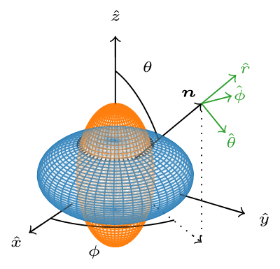
We represent the polarized radiation using the four element Stokes vector (Mishchenko et al., 2000, but noting the convention difference explained in Peest et al., 2017):

$$\mathbf{I}=\begin{pmatrix}I\\ Q\\ U\\ V\end{pmatrix}=\begin{pmatrix}E_{\theta{}}E^{*}_{\theta{}}+E_{\phi{}}E^{*}_{\phi{}}\\ E_{\theta{}}E^{*}_{\theta{}}-E_{\phi{}}E^{*}_{\phi{}}\\ E_{\theta{}}E^{*}_{\phi{}}+E_{\phi{}}E^{*}_{\theta{}}\\ i\left(E_{\phi{}}E^{*}_{\theta{}}-E_{\theta{}}E^{*}_{\phi{}}\right)\end{pmatrix},$$ (3)

where ^∗ represent the complex conjugate operation and we have assumed that the (generally complex) transverse components of the electromagnetic wave are expressed in a spherical right-handed coordinate frame $(\hat{r},\hat{\theta{}},\hat{\phi{}})$ with the radial direction along the propagation direction of the wave, pointing away from the origin (see Fig. 1). The vertical reference direction used to compute $\theta{}$ is given by an arbitrary north direction, which we will always choose to be along our $z$ axis. As a direct corollary, we will only have one linear polarization component, $Q$, while $U=0$ in all cases.

When an incoming plane electromagnetic wave with propagation direction $\boldsymbol{n}_{\rm{}i}=(\theta{}_{\rm{}i},\phi{}_{\rm{}i})$ scatters due to an interaction with a spheroidal dust particle with an orientation $\boldsymbol{n}_{\rm{}p}$ into a spherical wave with propagation direction $\boldsymbol{n}_{\rm{}s}$, its Stokes vector $\mathbf{I}^{\rm{}i}$ is converted into a new Stokes vector $\mathbf{I}^{\rm{}s}$. This new Stokes vector can be related to the original Stokes vector by means of the Müller matrix $\mathbf{M}(\boldsymbol{n}_{\rm{}s},\boldsymbol{n}_{\rm{}i};\boldsymbol{n}_{\rm{}p})$:

$$\mathbf{I}^{\rm{}s}=\frac{1}{R^{2}}\mathbf{M}(\boldsymbol{n}_{\rm{}s},\boldsymbol{n}_{\rm{}i};\boldsymbol{n}_{\rm{}p})\mathbf{I}^{\rm{}i},$$ (4)

where $R$ represents the linear distance traveled by the wave after scattering. Note that $\mathbf{M}$ has the dimensions of a surface area; it represents a scattering cross section.

Due to scattering, but also due to absorption of part of the electromagnetic energy within the scattering particle, a beam of light moving over a distance ${\rm{}d}s$ in a direction $\boldsymbol{n}$ through a medium consisting of spheroidal dust grains with the same orientation $\boldsymbol{n}_{\rm{}p}$ and density $n_{\rm{}p}$ will experience extinction, characterized by the extinction matrix $\mathbf{K}(\boldsymbol{n};\boldsymbol{n}_{\rm{}p})$:

$$\frac{{\rm{}d}\mathbf{I}}{{\rm{}d}s}=-n_{\rm{}p}\mathbf{K}(\boldsymbol{n};\boldsymbol{n}_{\rm{}p})\mathbf{I}.$$ (5)

Like the Müller matrix, the extinction matrix has the dimensions of a surface area.

To compute the absorption in a direction $\boldsymbol{n}$, we need to determine the absorption cross sections $\mathbf{K}_{\rm{}a}(\boldsymbol{n};\boldsymbol{n}_{\rm{}p})$ for the incoming Stokes vector components. This requires subtracting the total contribution of incoming waves scattering into the direction of interest from the relevant components of the extinction matrix:

$$K_{{\rm{}a},X}(\boldsymbol{n};\boldsymbol{n}_{\rm{}p})=K_{XI}(\boldsymbol{n};\boldsymbol{n}_{\rm{}p})-\int M_{XI}(\boldsymbol{n},\boldsymbol{n^{\prime}};\boldsymbol{n}_{\rm{}p}){\rm{}d}\boldsymbol{n}^{\prime},$$ (6)

where $X=I,Q,U,V$, and $M_{XI}$ represents the element of the matrix $\mathbf{M}$ that relates the incoming Stokes vector component $X$ to the outgoing Stokes vector component $I$.

In thermal equilibrium, the energy that is absorbed by the dust grains will be emitted again at different wavelengths. In this case, the absorption for the different Stokes vector components matches the corresponding emission, so once the absorption cross sections are known, the emission cross sections are also known.

The extinction and absorption cross sections are usually expressed as dimensionless quantities (extinction/absorption coefficients) by dividing by the cross section of a spherical grain with the same radius (Mishchenko, 1991):

$$Q_{\rm{}ext} =\frac{K_{II}}{\pi{}a^{2}}, Q_{\rm{}ext,pol}=\frac{K_{QI}}{\pi{}a^{2}},$$ (7)

$$Q_{\rm{}abs} =\frac{K_{{\rm{}a},I}}{\pi{}a^{2}}, Q_{\rm{}abs,pol}=\frac{K_{{\rm{}a},Q}}{\pi{}a^{2}}.$$ (8)

Calculation of the absorption and emission coefficients for a specific propagation direction hence requires the calculation of the extinction matrix for that direction, as well as the calculation of the Müller matrix for that outgoing direction integrated over all incoming directions. Additionally, the real interstellar medium does not consist of a single dust species with a fixed orientation, so that in general we need to replace the extinction and Müller matrices in these expressions with suitably ensemble averaged versions for a dust mixture with a specific size and shape distribution, and some prescribed alignment distribution.

To compute the elements of the extinction and Müller matrices, we need the complex forward scattering matrix $\mathbf{S}(\boldsymbol{n}_{\rm{}s},\boldsymbol{n}_{\rm{}i};\boldsymbol{n}_{\rm{}p})$ that links the transverse components of the electromagnetic field before and after the scattering event:

$$\begin{pmatrix}E^{\rm{}s}_{\theta}{}\\ E^{\rm{}s}_{\phi}{}\end{pmatrix}=\frac{1}{R}{\rm{}e}^{ikR}\mathbf{S}(\boldsymbol{n}_{\rm{}s},\boldsymbol{n}_{\rm{}i};\boldsymbol{n}_{\rm{}p})\begin{pmatrix}E^{\rm{}i}_{\theta}{}\\ E^{\rm{}i}_{\phi}{}\end{pmatrix},$$ (9)

where $k=|\boldsymbol{k}|$ is the norm of the wavenumber vector. This matrix can be calculated in various ways; we will use the so called T-matrix formalism (see Appendix A.1), which is based on an expansion of the incoming and outgoing electromagnetic waves in spherical basis functions. A powerful aspect of this formalism is that it allows for the construction of a single matrix $\mathbf{T}$ that encodes all properties for a dust mixture with a given alignment distribution around some reference direction, from which a single $\mathbf{S}$ matrix can be computed without the need for any additional averaging over particle orientations.

Once the $\mathbf{S}$ matrix is known within some reference frame, the extinction and Müller matrices within that same reference frame can be computed directly (Mishchenko et al., 2000):

$$M_{II} =\frac{1}{2}\left(|S_{\theta{}\theta{}}|^{2}+|S_{\theta{}\phi{}}|^{2}+|S_{\phi{}\theta{}}|^{2}+|S_{\phi{}\phi{}}|^{2}\right),$$ (10)

$$M_{IQ} =\frac{1}{2}\left(|S_{\theta{}\theta{}}|^{2}-|S_{\theta{}\phi{}}|^{2}+|S_{\phi{}\theta{}}|^{2}-|S_{\phi{}\phi{}}|^{2}\right),$$ (11)

$$M_{IU} ={\rm{}Re}\left(S_{\theta{}\theta{}}S^{*}_{\theta{}\phi{}}+S_{\phi{}\phi{}}S^{*}_{\phi{}\theta{}}\right),$$ (12)

$$M_{IV} =-{\rm{}Im}\left(S_{\theta{}\theta{}}S^{*}_{\theta{}\phi{}}-S_{\phi{}\phi{}}S^{*}_{\phi{}\theta{}}\right),$$ (13)

$$M_{QI} =\frac{1}{2}\left(|S_{\theta{}\theta{}}|^{2}+|S_{\theta{}\phi{}}|^{2}-|S_{\phi{}\theta{}}|^{2}-|S_{\phi{}\phi{}}|^{2}\right),$$ (14)

$$M_{QQ} =\frac{1}{2}\left(|S_{\theta{}\theta{}}|^{2}-|S_{\theta{}\phi{}}|^{2}-|S_{\phi{}\theta{}}|^{2}+|S_{\phi{}\phi{}}|^{2}\right),$$ (15)

$$M_{QU} ={\rm{}Re}\left(S_{\theta{}\theta{}}S^{*}_{\theta{}\phi{}}-S_{\phi{}\phi{}}S^{*}_{\phi{}\theta{}}\right),$$ (16)

$$M_{QV} =-{\rm{}Im}\left(S_{\theta{}\theta{}}S^{*}_{\theta{}\phi{}}+S_{\phi{}\phi{}}S^{*}_{\phi{}\theta{}}\right),$$ (17)

$$M_{UI} ={\rm{}Re}\left(S_{\theta{}\theta{}}S^{*}_{\phi{}\theta{}}+S_{\phi{}\phi{}}S^{*}_{\theta{}\phi{}}\right),$$ (18)

$$M_{UQ} ={\rm{}Re}\left(S_{\theta{}\theta{}}S^{*}_{\phi{}\theta{}}-S_{\phi{}\phi{}}S^{*}_{\theta{}\phi{}}\right),$$ (19)

$$M_{UU} ={\rm{}Re}\left(S_{\theta{}\theta{}}S^{*}_{\phi{}\phi{}}+S_{\theta{}\phi{}}S^{*}_{\phi{}\theta{}}\right),$$ (20)

$$M_{UV} =-{\rm{}Im}\left(S_{\theta{}\theta{}}S^{*}_{\phi{}\phi{}}+S_{\phi{}\theta{}}S^{*}_{\theta{}\phi{}}\right),$$ (21)

$$M_{VI} =-{\rm{}Im}\left(S_{\phi{}\theta{}}S^{*}_{\theta{}\theta{}}+S_{\phi{}\phi{}}S^{*}_{\theta{}\phi{}}\right),$$ (22)

$$M_{VQ} =-{\rm{}Im}\left(S_{\phi{}\theta{}}S^{*}_{\theta{}\theta{}}-S_{\phi{}\phi{}}S^{*}_{\theta{}\phi{}}\right),$$ (23)

$$M_{VU} =-{\rm{}Im}\left(S_{\phi{}\phi{}}S^{*}_{\theta{}\theta{}}-S_{\theta{}\phi{}}S^{*}_{\phi{}\theta{}}\right),$$ (24)

$$M_{VV} ={\rm{}Re}\left(S_{\phi{}\phi{}}S^{*}_{\theta{}\theta{}}-S_{\theta{}\phi{}}S^{*}_{\phi{}\theta{}}\right),$$ (25)

and

$$K_{XX} =\frac{2\pi{}}{k}{\rm{}Im}\left(S_{\theta{}\theta{}}+S_{\phi{}\phi{}}\right),$$ (26)

$$K_{IQ} =K_{QI}=\frac{2\pi{}}{k}{\rm{}Im}\left(S_{\theta{}\theta{}}-S_{\phi{}\phi{}}\right),$$ (27)

$$K_{IU} =K_{UI}=\frac{2\pi{}}{k}{\rm{}Im}\left(S_{\theta{}\phi{}}+S_{\phi{}\theta{}}\right),$$ (28)

$$K_{IV} =K_{VI}=\frac{2\pi{}}{k}{\rm{}Re}\left(S_{\phi{}\theta{}}-S_{\theta{}\phi{}}\right),$$ (29)

$$K_{QU} =-K_{UQ}=-\frac{2\pi{}}{k}{\rm{}Im}\left(S_{\phi{}\theta{}}-S_{\theta{}\phi{}}\right),$$ (30)

$$K_{QV} =-K_{VQ}=-\frac{2\pi{}}{k}{\rm{}Re}\left(S_{\theta{}\phi{}}+S_{\phi{}\theta{}}\right),$$ (31)

$$K_{UV} =-K_{VU}=-\frac{2\pi{}}{k}{\rm{}Re}\left(S_{\phi{}\phi{}}-S_{\theta{}\theta{}}\right).$$ (32)

2.2 Scattering correction

Once the extinction and scattering matrices are known, the computation of the absorption coefficients can be done using a numerical integration over all angles. To this end, we use Gauss-Legendre quadrature on a grid in $(\cos{}\theta{},\phi{})$ space (see Section B.2). This kind of numerical quadrature lends itself well for integration over functions that are smooth functions of direction, and is also extensively used in the T-matrix calculation itself (see Section A.1).

To quantify the accuracy of our numerical integration scheme, we will compute the absorption coefficients for a large silicate dust grain ($1~{}\mu{}$m) and for the shortest wavelength in our range of interest ($10~{}\mu{}$m), since these parameters are the most challenging to compute. For the same reason, we will focus on prolate and oblate grains at the edges of the integration range for our assumed shape distribution (see Section 2.4), i.e. $d_{\rm{}prol}=0.19$, $d_{\rm{}obl}=6.96$. We will then increase the number of Gauss-Legendre quadrature points and see how the absorption coefficients converge.

Figure 2: Top: Convergence of the absorption coefficients with the number of quadrature points used to compute the scattering correction term. Bottom: Mean and maximum relative error for the same coefficients as a function of number of quadrature points. The relative error is computed w.r.t. the mean of the corresponding quantity, using the values obtained with $20^{2}$ quadrature points as a reference.

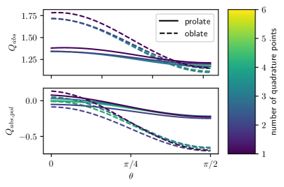
The results of this convergence test are shown in Fig. 2. The top panel shows the visual convergence by overplotting results for different numbers of quadrature points (the number that is quoted corresponds to the number for one of the spherical coordinates; we sample that number of points in both the azimuth angle $\phi{}$ and the projected zenith angle $\theta{}$, so the total number of quadrature points is the square of that number). Due to the smooth nature of the Müller matrix for these input values, convergence is very quick. This is quantified in the bottom panel, where we show the relative error for the two absorption coefficients over the full $\theta{}$ range w.r.t. the result obtained using $20^{2}$ quadrature points. This corresponds to the value we will use in the rest of this work.

2.3 Orientation and alignment

Since CosTuuM is primarily aimed at studying the polarization signature in thermal emission from aligned dust grains, we have to consider a range of possible alignment strengths. Note that we make no assumptions about possible alignment mechanisms: it is the responsibility of the user to choose an appropriate mechanism for a given grain size, material type and wavelength within the astrophysical context of interest.

Within our implementation, the alignment of grains is governed by two independent distributions: an alignment distribution that specifies the alignment strength for grains of different sizes and compositions, and an orientation distribution that expresses the grain alignment for one set of these parameters as a function of alignment angle. Both of these can be customized within the CosTuuM framework and we only consider a small set of examples. For the alignment distribution, we will assume that only silicate grains with radii larger than a threshold radius of $0.1~{}\mu{}$m are aligned, consistent with models that show alignment is small for grains with sizes smaller than $0.05~{}\mu{}$m (Kim & Martin, 1995; Draine & Fraisse, 2009), and with the self-consistently computed alignment thresholds from Reissl et al. (2016).

Due to symmetry, it is generally possible to express the orientation of any spheroid w.r.t. the direction of the magnetic field by means of a single angle $\beta{}$, the angle between the magnetic field direction and the symmetry axis of the spheroid. The various orientations of the ensemble of grains can then be captured via a distribution $p(\beta{})$, normalized such that

$$\int_{0}^{\pi{}}p(\beta{})\sin\beta{}{\rm{}d}\beta{}=1.$$ (33)

We follow Mishchenko (1991) and focus on three distinct types of distributions. For grains with a random orientation (no alignment), the distribution function is uniform and given by

$$p(\beta{})=\frac{1}{2}.$$ (34)

If the grains are perfectly aligned (this is also called Davis-Greenstein alignment), the distribution is a Dirac delta distribution:

$$p(\beta{}) =\delta{}\left(\beta{}-\frac{\pi{}}{2}\right), {\rm{}(prolate)}$$ (35)

$$p(\beta{}) =\delta{}\left(\beta{}\right). {\rm{}(oblate)}$$ (36)

Mishchenko (1991) finally introduces a distribution for imperfectly aligned grains, given by (note the factor $3$ that is missing in the original work)

$$p(\beta{})=\frac{1}{2}+\frac{5}{4}p_{2}\left(3\cos^{2}\beta{}-1\right),$$ (37)

where $p_{2}\in{}\left[-1/5,2/5\right]$ is a free parameter. Like Mishchenko (1991), we use $p_{2}=-1/5$ for prolate grains and $p_{2}=2/5$ for oblate grains. We will refer to this distribution as the Mishchenko distribution.

As in Mishchenko (1991) we expand the orientation distribution in Legendre polynomials and use the expansion coefficients to compute the T-matrix for the ensemble of grains. This procedure has been implemented in such a way that users can provide their own expression for the orientation distribution, and we have successfully tested it with alternative distributions that have the shape of a normal distribution.

2.4 Shape distribution

Previous studies have mainly considered a single shape of aligned grains (Siebenmorgen et al., 2014; Reissl et al., 2016; Bertrang & Wolf, 2017), with a preference for oblate grains with relatively moderate axis ratios. A real population of grains can be expected to have a more general distribution $P(d)$ of shapes. Expressions for these shape distributions can be found in literature (Min et al., 2003), we will adopt the general Continuous Distribution of Ellipsoids (CDE) given in Draine & Hensley (2017). Their favored CDE, labeled CDE2, is given in terms of the shape factors $L_{i},i=1,2,3$:

$$G(L_{1},L_{2})=120L_{1}L_{2}L_{3}=120L_{1}L_{2}(1-L_{1}-L_{2}),$$ (38)

where the shape factors are linked to the axis ratio $d$ through

$$L_{1}=L_{3}=\frac{1-L_{2}}{2}$$ (39)

and

$$L_{2} =\frac{1-e^{2}}{e^{2}}\left[\frac{1}{2e}\ln\left(\frac{1+e}{1-e}\right)-1\right],$$ (40)

$$e^{2} =1-d^{2},$$ (41)

for prolate spheroids ($d<1$) and

$$L_{2} =\frac{1}{e^{2}}\left[1-\frac{\sqrt{1-e^{2}}}{e}\arcsin{}e\right],$$ (42)

$$e^{2} =1-\frac{1}{d^{2}},$$ (43)

for oblate spheroids ($d>1$) (Min et al., 2003).

To obtain a practical expression for $P(d)$ based on the general expression $G(L_{1},L_{2})$, we first substitute $L\equiv{}L_{2}$

$$G(L)=12L(1-L)^{2},$$ (44)

where the normalization constant was chosen such that $\int_{0}^{1}G(L){\rm{}d}L=1$. For each value of $d\in{}[0,\infty{}[$, we can determine the shape factor $L$ and the corresponding CDE2 probability density. To turn this into a probability density function for the coordinate $d$, we need to multiply with the Jacobian (Min et al., 2003)

$$\frac{{\rm{}d}L}{{\rm{}d}d}=\frac{\sqrt{1-e^{2}}}{2e^{5}}\left[(3-e^{2})\ln\left(\frac{1+e}{1-e}\right)-6e\right]$$ (45)

for prolate spheroids and

$$\frac{{\rm{}d}L}{{\rm{}d}d}=\frac{1-e^{2}}{e^{5}}\left[(3-2e^{2})\arcsin{}e-3e\sqrt{1-e^{2}}\right]$$ (46)

for oblate spheroids.

Figure 3: Shape distribution as a function of axis ratio, $d$. Shown are the Draine & Hensley (2017) CDE2 distribution and the Min et al. (2003) CDS distribution. The shaded area underneath the CDE2 curve corresponds to the 96 % of the distribution that we actually sample in our runs.

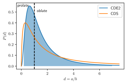
The corresponding distribution function as a function of the axis ratio $d$ is shown in Fig. 3. Also shown is the continuous distribution of spheroids (CDS) expression given in Min et al. (2003) that assumes a uniform weight for all values of $L$. While in the latter, $1/3$ of the grains are prolate, the CDE2 distribution has relatively less extreme axis ratios, so that $\approx{}40$ % of the grains is prolate.

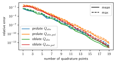
As for the scattering correction, we will numerically average the absorption coefficients over the shape distribution using Gauss-Legendre quadrature. This procedure is novel for our method, and hence no comparison results are available in literature. We can check the accuracy of our implementation in two steps. First, we need to show that our numerical quadrature rule is implemented correctly. This can be done by replacing the input absorption coefficients and the assumed shape distribution with known analytic functions, and checking against the expected analytic result. This is a trivial exercise. Second, we need to check that our results are converged for the choice of parameters we make for the numerical quadrature. This can again be achieved by increasing the number of quadrature points until convergence is reached.

Figure 4: Top: Convergence of the absorption coefficients with the number of quadrature points used to compute the shape distribution average. Bottom: Mean and maximum relative error for the same coefficients as a function of number of quadrature points. The relative error is computed w.r.t. the mean of the corresponding quantity, using the values obtained with 20 quadrature points as a reference.

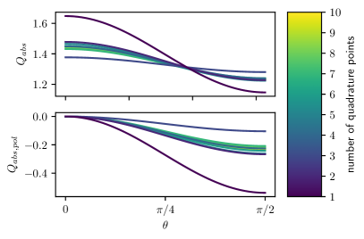
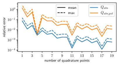
Fig. 4 shows the convergence results for this test. Since in this case every sample in shape space corresponds to a separate T-matrix calculation, the absolute error is quickly dominated by the error on a single T-matrix calculation. For the absorption coefficient, we can achieve a relative error of $\approx{}10^{-3}$. For the polarized absorption coefficient we achieve a similar absolute error, but since the actual values are lower, we are limited to a relative error of a few percent.

Figure 5: Top: Convergence of the absorption coefficients with the fraction of the shape distribution that gets sampled. Bottom: Mean and maximum relative error for the same coefficients as a function of sampling fraction. The relative error is computed w.r.t. the mean of the corresponding quantity, using the values computed with a sampling fraction $f_{S}=0.97$ as a reference.

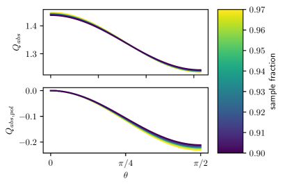
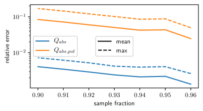
Another issue to address is the fraction of the shape distribution that we need to sample to get consistent absorption coefficients. In principle, the shape distribution is defined for axis ratio values $d\in{}[0,\infty{}[$, but the T-matrix method runs into numerical issues for axis ratio values close to both ends of that interval. We therefore determine new limits, $[d_{l},d_{u}]$ so that we sample a representative fraction $f_{S}$ of the CDE2 distribution on both ends of the axis $d=1$:

$$f_{S}=\frac{\int_{d_{l}}^{1}P(d){\rm{}d}d}{\int_{0}^{1}P(d){\rm{}d}d}=\frac{\int_{1}^{d_{u}}P(d){\rm{}d}d}{\int_{1}^{\infty}{}P(d){\rm{}d}d}$$ (47)

and assume the entire distribution can be approximated by this value.

Fig. 5 shows the absorption coefficients for various fractions of the sampling interval, for the same challenging grain size and wavelength as used above. The method breaks down for fractions larger than 97 %. It is clear that our results are still dependent on the sampling fraction for that value, but the dependence is only of the order of 10 % for the most extreme zenith angles, and overall the results are reasonably converged. We therefore settle on a value of 96 % for all our calculations. Note that the numerical issues reduce the fraction we can sample quickly once $\lambda{}$ decreases: for a grain size of $a=1~{}\mu{}$m, we can only sample 80 % of the distribution at $\lambda{}=1~{}\mu{}$m, and this even goes down to 50 % at $\lambda{}=0.3~{}\mu{}$m. As shown by Somerville et al. (2013), these issues can be alleviated by making some changes to the core of the T-matrix algorithm, should this be required in the future.

2.5 Grain properties

Apart from the alignment and shape properties already mentioned above, we also need to specify the material properties (refractive index) and size distribution for the dust grains. For the former, we are limited to tabulated values available in literature, e.g. Draine (1985). Alternatively, we also made it possible to pass on custom material properties to the CosTuuM library.

Since grain sizes are a function of position in many contemporary RT methods, we do not integrate the optical properties over a grain size distribution within CosTuuM and leave this to the application. However, to illustrate the impact of a grain mixture of different sizes on the results shown in Section 3, we will assume a basic MRN power-law grain size distribution (Mathis et al., 1977):

$$\Omega{}(a)\propto{}a^{-3.5},a\in{}[a_{\rm{}min},a_{\rm{}max}].$$ (48)

Following Reissl et al. (2016), we set $a_{\rm{}min}=5$ nm and $a_{\rm{}max}=2~{}\mu{}$m. This additional grain size averaging procedure is not part of CosTuuM, and was entirely implemented using Python’s NumPy library.

3 Results and discussion

In this section, we will apply CosTuuM to a range of scenarios to illustrate its validity and accuracy, and to explore the impact of some commonly made assumptions about the properties of spheroidal dust grains.

3.1 Mishchenko extinction results

Mishchenko (1991) contains a small number of reference values for the extinction coefficients, computed using the same T-matrix formalism used by CosTuuM. Reproducing these values correctly is a good test for the T-matrix formalism itself and for the procedure to average over different particle orientations (a part not available in the public version of Mishchenko’s code).

The test assumes a single silicate dust grain with a radius of $0.2~{}\mu{}$m that is either prolate with an axis ratio $d=1/2$ or oblate with an axis ratio $d=2$. For both grains, the three different alignment distributions are compared: random orientation (no alignment), perfect (Davis-Greenstein) alignment, and Mishchenko alignment.

For perfect and imperfect alignment, the extinction coefficients become dependent on the angle between the direction of the magnetic field and the incoming electromagnetic wave, so values are listed for 4 different angles: $\theta{}=\{0,\pi{}/6,\pi{}/3,\pi{}/2\}$. The refractive index of the grain is set to the values from Draine (1985), which differ slightly from the values given on Bruce Draine’s web page that are also used in Section 3.3.

Figure 6: Extinction coefficient (top row) and linearly polarized extinction coefficient (bottom row) as a function of zenith angle $\theta{}$, for a silicate dust grain with an equal volume radius $0.2~{}\mu{}$m, and for four different incoming wavelengths and two different axis ratios, as indicated in the legend. The three columns correspond to three different alignment distributions. The symbols correspond to the values from Mishchenko (1991), while the lines were computed with CosTuuM on a linear $\theta{}$ grid with 100 values.

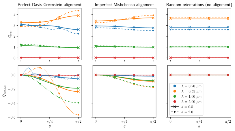
The results of the tests are shown in Fig. 6. The results are in clear agreement for all wavelengths and both axis ratios, and for all alignment cases. Due to the significant improvements in computational power, we can now very easily compute these values for many more angles than in the original work by Mishchenko (1991).

For long wavelengths and small dust grains (or small values of the size parameter $x_{V}=2\pi{}a/\lambda{}$, commonly used in literature), scattering by dust becomes negligible, so the extinction coefficients in this regime will be equal to the absorption coefficients. In this regime, this test hence directly tests the validity of the absorption coefficients. However, for shorter wavelengths, this approximation no longer holds and we need to also take into account the scattering correction term in equation (6). We need to test this part of the algorithm separately.

3.2 Voshchinnikov extinction results

Voshchinnikov & Farafonov (1993) present another set of reference results for the extinction coefficients, this time computed using the SVM method. Their results do not include any orientation averaging, but provide an independent benchmark test for the results of an individual scattering calculation. We present three different tests, respectively corresponding to Figs. 3-5 in Voshchinnikov & Farafonov (1993). We compare CosTuuM results with results obtained using the public version of the Voshchinnikov & Farafonov (1993) code. All these tests use a fixed photon wavelength $\lambda{}=0.5~{}\mu{}$m.

Figure 7: Extinction coefficient as a function of zenith angle $\theta{}$, for a single spheroidal dust grain that has its symmetry axis oriented along the positive $z$ axis. The shape and refractive index of the grain are indicated above each panel, while the grain size is indicated in the legend. Full lines correspond to results computed with CosTuuM, while the symbols are the results from Voshchinnikov & Farafonov (1993). All results use a photon wavelength $\lambda=0.5~{}\mu{}$m.

The first test evaluates the zenith angle dependence of the extinction coefficient $Q_{ext}$ for five different grain sizes ($a\in{}[0.05,0.10,0.15,0.20,0.25]~{}\mu{}$m), and for moderate axis ratios, $d=1/2$ and $d=2$. Results are obtained for prolate grains with refractive index $m_{r}=1.31+0.01i$ and $m_{r}=1.70+0.03i$, while only the former value is used for the oblate spheroid. As shown in Fig. 7, our results are in excellent agreement.

Figure 8: Polarized extinction coefficient as a function of zenith angle $\theta{}$, for a single spheroidal dust grain that has its symmetry axis oriented along the positive $z$ axis. The refractive index of the grain is indicated above each panel, while the shape is indicated in the legend. Full lines correspond to results computed with CosTuuM, while the symbols are the results from Voshchinnikov & Farafonov (1993). All results use a grain size $a=0.25~{}\mu{}$m and photon wavelength $\lambda{}=0.5~{}\mu{}$m.

The second test looks at the zenith angle dependence of the polarized exinction coefficient $Q_{ext,pol}$ for different axis ratios $d$, and uses a single grain size $a=0.25~{}\mu{}$m and refractive indices $m_{r}=1.31+0.01i$ (for both prolate and oblate grains) and $m_{r}=1.70+0.03i$ (prolate grains only). Fig. 8 again shows excellent agreement.

Figure 9: Extinction coefficient (top) and polarized extinction coefficient (bottom) as a function of (inverse) axis ratio $d$, for a single spheroidal dust grain that has its symmetry axis oriented along the positive $z$ axis. Results are shown for two zenith angles $\theta{}$, as indicated in the legend. Full lines correspond to results computed with CosTuuM, while the symbols are the results from Voshchinnikov & Farafonov (1993). All results use a refractive index $m_{r}=1.31+0.01i$, grain size $a=0.25~{}\mu{}$m and photon wavelength $\lambda{}=0.5~{}\mu{}$m. To facilitate comparison with Voshchinnikov & Farafonov (1993), the inverse axis ratio is plotted for the prolate grains.

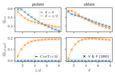
The final test considers the axis ratio dependence of both $Q_{ext}$ and $Q_{ext,pol}$ at zenith angles $\theta{}=0$ and $\theta{}=\pi{}/2$, for a single grain with size $a=0.25~{}\mu{}$m and refractive index $m_{r}=1.31+0.0i$. As seen in Fig. 9, we obtain excellent agreement over the full range $d\in{}[0.13,8.00]$.

3.3 Draine dust models

To test the calculation of absorption coefficients (including the scattering correction), we compare with the publicly available values of Draine & Lee (1984); Laor & Draine (1993). They provide values for a large wavelength range and for a number of grain sizes, but only for spherical grains.

Figure 10: Absorption coefficient as a function of wavelength for a single spherical silicate dust grain. The different lines compare the original Laor & Draine (1993) with values calculated using CosTuuM, with and without the additional scattering correction term.

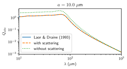
Fig. 10 shows an example for one grain size for a limited wavelength range, and shows the impact of including the scattering correction, especially at shorter wavelengths. Note that the T-matrix method becomes unstable for short wavelengths and large grain sizes, so that our CosTuuM calculations are necessarily limited to this range. This is not an issue, since thermal dust emission becomes negligible for short wavelengths.

Figure 11: Ratio of the absorption coefficient for spheroidal grains and for spherical grains with the same equal volume radius, as a function of wavelength, and for three different shapes, as indicated in the legend.

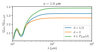
Fig. 11 shows the ratio of the absorption coefficients for spheroidal grains and for spherical grains with the same equal volume radius, for a pure oblate ($d=2$) and pure prolate ($d=1/2$) silicate grain and for a realistic mixture of grains with the shape distribution given by equations (44)-(46). Note that the ratios are always larger than one, indicating that spheroidal grains are more efficient absorbers than the equivalent spherical grains. Moreover, the grains with shapes distributed according to the CDE2 distribution have significantly higher absorption coefficients, since their average value is dominated by oblate spheroids with relatively large axis ratios.

One explanation for this increased efficiency is that the definition of the absorption/extinction coefficient given by equations (7)-(8) ignores the fact that spheroidal grains have a larger active surface area, i.e. the total average projected surface area seen by photons that are incoming from all sides is always larger for spheroidal grains than for a sphere with the same volume. As a result, the absorption coefficients for both oblate and prolate spheroidal grains are always larger than for a spherical grain with the same volume. We can correct for this effect by multiplying with the corresponding correction factor,

$$C_{A}=\left(\frac{d^{-1/3}}{2}\int_{-1}^{1}\sqrt{\frac{(d^{4}-1)x^{2}+1}{(d^{2}-1)x^{2}+1}}dx\right)^{-1}.$$ (49)

This expression can be derived using basic geometrical algebra (Vickers & Brown, 2001).

Figure 12: Ratio of the absorption coefficient for spheroidal grains and for spherical grains with the same equal volume radius, as a function of wavelength, corrected to account for the higher average projected surface area. To eliminate additional differences because of the size dependence of the refractive index, we assume a constant refractive index.

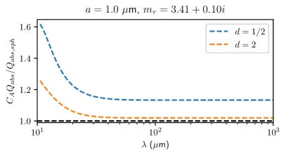
To test that this is indeed the case, we need to eliminate all other differences in the calculation for the absorption coefficient, i.e. we need to make sure we use a constant refractive index. Fig. 12 shows the results for a refractive index $m_{r}=3.41+0.10i$ (corresponding to the Laor & Draine (1993) value for $\lambda{}=500~{}\mu{}$m), this time corrected with the $C_{A}$ factor. The corrected absorption coefficients get closer to the values for the equivalent spherical grains, although they are still higher; this is a manifestation of the extinction paradox (Bohren & Huffman, 1983). The offset gets larger when the wavelength of the incoming radiation gets closer to the size of the particle due to non-linear effects.

For an assumed constant grain composition, the mass of the dust grain is proportional to its volume. So the different absorption coefficients can be readily compared if we assume a constant dust mass. As can be seen from Fig. 11, dust absorption and emission are stronger for spheroidal dust grains.

Figure 13: Maximum relative difference between CosTuuM absorption coefficients and the values presented by Draine & Lee (1984); Laor & Draine (1993) as a function of grain size, for three different grain types available on Bruce Draine’s web page, as indicated in the legend.

Figure 14: Absorption coefficient as a function of wavelength for carbon dust grains with the size indicated in the title. The different colors correspond to different CosTuuM models and the reference values from Draine & Lee (1984), as indicated in the legend. The $1/3-2/3$ CosTuuM model corresponds to the weighted average of the $\varepsilon{}\parallel{}c$ and $\varepsilon{}\perp{}c$ models, whereby the former have $1/3$ of the weight and the latter the other $2/3$.

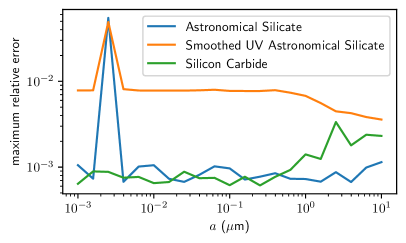
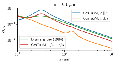
Fig. 13 shows the relative difference between the CosTuuM absorption coefficients and the reference models computed by Draine & Lee (1984); Laor & Draine (1993), as a function of grain size and for various grain compositions. Overall, the relative error is low, so that we can conclude that CosTuuM reproduces the existing optical properties results very well. A notable exception is carbon (see Fig. 14), for which CosTuuM systematically under predicts the absorption coefficient for long wavelengths and over predicts some features at shorter wavelengths. As pointed out by Draine & Lee (1984), carbon is a highly anisotropic material, so that its dielectric function is in fact a tensor; this tensor is usually represented in its diagonal form, with one diagonal element parallel to the incident electromagnetic field ($\varepsilon{}\parallel{}c$), and two elements perpendicular to it ($\varepsilon{}\perp{}c$). The optical properties of carbon are then computed by taking an ad-hoc $1/3$-$2/3$ mixture of the optical properties computed for both values of the refractive index. On top of that, carbon is a dielectric material with a non-negligible magnetic dipole absorption, which is not treated accurately by the T-matrix method.

3.4 Polarized dust emission

Now that we have shown that CosTuuM generates accurate results in the infrared wavelength regime, we can use it to make predictions for the absorption cross sections for a reference silicate grain model with an MRN size distribution, $\Omega{}(a)=a^{-3.5}$, a CDE2 shape distribution, and perfect grain alignment. We will compute the size-averaged absorption cross sections

$$\langle{}K_{a,I}\rangle{}(\lambda{},\theta{}) =\int_{a_{\rm{}min}}^{a_{\rm{}max}}\Omega{}(a)Q_{\rm{}abs}(\lambda{},a,\theta{})\pi{}a^{2}{\rm{}d}a,$$ (50)

$$\langle{}K_{a,Q}\rangle{}(\lambda{},\theta{}) =\int_{a_{\rm{}min}}^{a_{\rm{}max}}\Omega{}(a)Q_{\rm{}abs,pol}(\lambda{},a,\theta{})\pi{}a^{2}{\rm{}d}a.$$ (51)

We will evaluate these functions at three representative wavelengths: $70~{}\mu{}$m, $200~{}\mu{}$m and $350~{}\mu{}$m. These correspond to the peak wavelengths for black-body emission at $72.9$ K, $25.5$ K and $14.6$ K, and are also the centers of the bands for the B-BOP polarimeter on board the proposed ESA/JAXA M5 mission SPICA (Roelfsema et al., 2018; André et al., 2019). We will only show the zenith angle range $[0,\pi{}/2]$, since our results are symmetric w.r.t. the $\theta{}=\pi{}/2$ axis. Independent of the assumed alignment mechanism, all our results assume a magnetic field directed along the positive $z$ axis with $\theta{}=0$.

As in Peest et al. (2017), we will characterize the strength of the polarization using the degree of linear polarization,

$$P_{L}=\frac{\sqrt{Q^{2}+U^{2}}}{I}=\frac{\left|\langle{}K_{a,Q}\rangle{}(\lambda{},\theta{})\right|}{\langle{}K_{a,I}\rangle{}(\lambda{},\theta{})},$$ (52)

where in the second step we have assumed that the observed intensities are directly proportional to the emitted intensities and are observed with an instrument that has its north direction parallel to the orientation of the magnetic field, so that $U=0$. The linear polarization angle

$$\gamma{}=\frac{1}{2}\arctan\left(\frac{U}{Q}\right)$$ (53)

is in this case trivially 0.

Figure 15: Size-averaged absorption cross section (top), polarized absorption cross section (middle) and linear polarization fraction (bottom) as a function of zenith angle $\theta{}$ for our fiducial model using a CDE2 shape distribution and assuming perfect grain alignment above a threshold grain size of $0.1~{}\mu{}$m. The different colors correspond to the three different wavelengths for the planned B-BOP polarimeter.

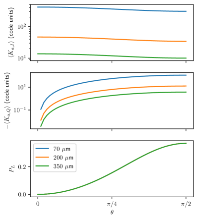
The results for our fiducial model are shown in Fig. 15. There is no linear polarization along the direction of the magnetic field; the linear polarization is maximal when the grains are observed in a direction perpendicular to the magnetic field direction. The three wavelengths shown have identical linear polarization fractions. This can be explained by the small difference in refractive index between these three wavelengths. The total absorption and hence emission coefficient does increase significantly at shorter wavelengths. Below, we will hence mainly focus on results for $\lambda{}=200~{}\mu{}$m.

3.5 Alignment distribution

Various methods to approximate the absorption coefficients for partially aligned spheroidal grains have been discussed in literature. Dyck & Beichman (1974) introduced a heuristic approximation whereby a fraction $f_{a}$ of the grains is perfectly aligned, and the rest has a random orientation. They do however rely on an approximate calculation of the absorption coefficients for aligned grains, and do not provide a recipe to relate the alignment fraction to a specific alignment mechanism. Draine & Allaf-Akbari (2006); Draine & Fraisse (2009) use so called picket fence alignment to compute the average extinction and absorption cross section over all angles, whereby the alignment of the dust grains is given in terms of a single alignment fraction $f_{\rm{}pf}$ so that a fraction $(1+2f_{\rm{}pf})/3$ of the grains has their short axis aligned with the magnetic field, while the remaining grains have their short axis aligned with two mutually orthogonal directions that are both perpendicular to the magnetic field direction in equal proportions.

This approach is similar to Reissl et al. (2016), who go a step further and self-consistently compute the alignment based on the local radiation field and dust properties. They parameterize the alignment using the Rayleigh reduction factor,

$$R=\left\langle{}\left(\frac{3}{2}\cos^{2}\beta{}-\frac{1}{2}\right)\left(\frac{3}{2}\cos^{2}\zeta{}-\frac{1}{2}\right)\right\rangle{},$$ (54)

where $\beta{}$ is the angle between the magnetic field and the angular momentum vector of the aligning grain, and $\zeta{}$ the angle between the angular momentum vector and the short axis of the spheroidal grain, the so called internal alignment angle. If we assume perfect internal alignment, then $\zeta{}=0$ and the Rayleigh reduction factor reduces to

$$R=\frac{3}{2}\langle{}\cos^{2}\beta{}\rangle{}-\frac{1}{2},$$ (55)

which is similar to the parametrization for alignment distributions used by Mishchenko (1991) (in fact, the Rayleigh reduction factor $R$ is equal to twice the expansion coefficient parameter $p_{2}$ for Mishchenko’s imperfect alignment distribution; the factor 2 stems from a different normalization for the angular average).

Once the Rayleigh reduction factor is known, the absorption coefficients are given by

$$Q_{\rm{}abs}(\theta{})=\langle{}Q\rangle{}+R(Q_{\parallel{}}-Q_{\perp{}})\left(\frac{1}{3}-\frac{1}{2}\sin^{2}\theta{}\right),$$ (56)

$$Q_{\rm{}abs,pol}(\theta{})=-\frac{1}{2}R(Q_{\parallel{}}-Q_{\perp{}})\sin^{2}\theta{},$$ (57)

with

$$\langle{}Q\rangle{}=\frac{2Q_{\perp{}}+Q_{\parallel{}}}{3},$$ (58)

$$Q_{\perp{}}=Q_{\rm{}abs}\left(\theta{}=\frac{\pi{}}{2}\right),$$ (59)

$$Q_{\parallel{}}=Q_{\rm{}abs}(\theta{}=0),$$ (60)

where for the last two equations we do not assume any alignment with a magnetic field, but evaluate the absorption coefficient in a frame where the $z$ axis corresponds to the symmetry axis of the dust grain. Note that the expression for $\langle{}Q\rangle{}$ is different from the one given by Reissl et al. (2016) (see also Lee & Draine, 1985; Draine & Fraisse, 2009). Similarly, there is a sign difference in the expression for $Q_{\rm{}abs,pol}$. These approximate expressions are valid in the Rayleigh limit, i.e. for grain sizes that are significantly smaller than the wavelength of the absorbed radiation.

If we average the expressions for $Q_{\rm{}abs}(\theta{})$ and $Q_{\rm{}abs,pol}(\theta{})$ over all zenith angles $\theta{}$, we find

$$\langle{}Q_{\rm{}abs}\rangle{} =\langle{}Q\rangle{},$$ (61)

$$\langle{}Q_{\rm{}abs,pol}\rangle{} =\frac{R}{3}(Q_{\parallel{}}-Q_{\perp{}}).$$ (62)

The Rayleigh reduction factor has the same meaning as the alignment fraction $f_{\rm{}pf}$ for picket fence alignment (Draine & Fraisse, 2009).

We will perform two tests. In the first test, we will compute the average absorption coefficients for a specific grain alignment using picket fence alignment, and a full angular averaging for both the mixture of random and perfectly aligned grains and imperfectly aligned grains. In the second test, we will compute the zenith angle dependence of the absorption coefficients using a mixture of random and perfect alignment, using picket fence alignment, and using Mishchenko (1991) imperfect alignment with CosTuuM, for a range of alignment fractions and equivalent Rayleigh reduction factors. Since all these methods to some extent require information about the shape (prolate or oblate) and assume a uniform alignment mechanism for all sizes, we will show results for a single grain size ($1~{}\mu{}$m) and for two fixed shapes: $d=0.5$ (prolate) and $d=2$ (oblate).

3.5.1 Average absorption cross section

Figure 16: Angular averaged absorption coefficient (top) and linear polarization fraction (bottom) for prolate (left) and oblate (right) grains as a function of wavelength, computed using various methods, as indicated in the legend.

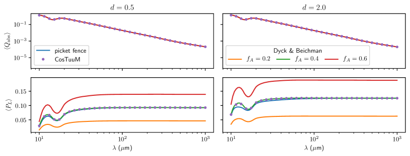
Fig. 16 shows the angular averaged absorption coefficient and linear polarization fraction for our representative grains as a function of wavelength, calculated using the various methods. We assume all grains are imperfectly aligned according to a Mishchenko alignment distribution with $p_{2}=-0.2$ (prolate) and $p_{2}=0.4$ (oblate), corresponding to Rayleigh reduction factors $R=-0.4$ and $R=0.8$ respectively. As expected, all methods show excellent agreement for the average absorption coefficient. Both picket fence alignment and the mixture of perfectly aligned and randomly aligned grains provide good approximations for the average linear polarization fraction at long wavelengths, where the Rayleigh approximation is valid. Towards shorter wavelengths, discrepancies start to appear between the picket fence alignment result and the CosTuuM-based results, as the Rayleigh approximation starts to break down. The fully self-consistent CosTuuM results are exactly reproduced by assuming a mixture with a polarized fraction $f_{A}=0.4$, so a dust grain mixture with imperfectly aligned grains can be reliably reproduced using this approximation. Note however that there is no general recipe to relate the alignment fraction $f_{A}$ to the parameters of the orientation distribution, and that computing the absorption coefficients as a function of zenith angle for perfectly aligned grains is equally complex as computing them for an imperfectly aligned ensemble. So this approximation has no real benefits.

3.5.2 Zenith angle dependence

Figure 17: Linear polarization fraction for prolate (left) and oblate (right) grains as a function of zenith angle, computed using various methods, as indicated in the legend. Top: values for $\lambda{}=10~{}\mu{}$m, bottom: values for $\lambda{}=205~{}\mu{}$m.

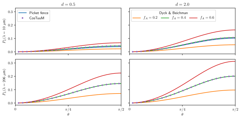
Fig. 17 shows the zenith angle dependence of the linear polarization fraction for the same representative grains, and for two representative wavelengths: a long wavelength for which both picket fence alignment and a mixture of random and perfect alignment provide excellent approximations, and a shorter wavelength for which picket fence alignment starts to diverge. Picket fence alignment underestimates the linear polarization fraction perpendicular to the orientation of the magnetic field, which explains the systematic underestimation of the average linear polarization fraction we found above.

In this case, using the Dyck & Beichman (1974) approximation does have a clear numerical advantage: by calculating the zenith angle dependence for the perfectly aligned case, we can represent the correct zenith angle dependence for any other alignment case, assuming we have a method to determine the corresponding $f_{A}$.

3.6 Shape distribution

The shape of spheroidal dust grains is poorly constrained, and most authors therefore tend to assume a single shape for their spheroidal dust grains, with a preference for oblate spheroids with $d=2$ (Draine & Lee, 1984; Draine & Allaf-Akbari, 2006; Reissl et al., 2016; Bertrang & Wolf, 2017; Reissl et al., 2018). Siebenmorgen et al. (2014) explore some more extreme axis ratios ($d\in{}[2,3,4]$), while Kim & Martin (1995) even discuss prolate grains with $d\in{}[1/2,1/4]$. Studies that try to fit dust properties to observations tend to prefer oblate grains with smaller axis ratios, $d=3/2$ (Draine & Malhotra, 1993), $d=\sqrt{2}$ (Draine & Allaf-Akbari, 2006), $d\in{}[1.4,1.6]$ (Draine & Fraisse, 2009).

Min et al. (2003) and Draine & Hensley (2017) address the issue of shape effects and describe the use of more general shape distributions like the CDE2 distribution we use here, but they do not explore the differences between this full statistical sampling and the use of a single shape, nor do they show that a single shape can in fact represent an ensemble of grains accurately.

Figure 18: Size-averaged absorption cross section (top) and linear polarization fraction (bottom) as a function of zenith angle $\theta{}$ for various single shape grains as indicated in the figure, and for our fiducial CDE2 shape distribution. All results are shown for a wavelength of $200~{}\mu{}$m.

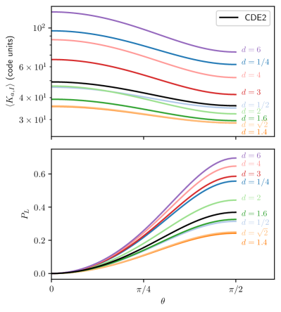
In Fig. 18 we show the absorption cross section and linear polarization fraction as a function of zenith angle for our fiducial dust grain mixture at $\lambda{}=200~{}\mu{}$m, and for various assumed grain shapes and our CDE2 mixture. Perfect grain alignment is assumed. None of the assumed single shape results matches the CDE2 mixture; while the absorption coefficient is larger than that for a $d=2$ grain shape, the linear polarization fraction is relatively low, in between the $d=1.6$ and $d=2$ result. Assuming a single shape will hence underestimate the emission and overestimate the polarization. It is also clear that the zenith angle dependence of the CDE2 distribution result is more similar to the oblate than to the prolate grain shapes, so the assumption of a single oblate shape is more justified. This is to be expected, as the average shape $\langle{}d\rangle{}$ for the CDE2 distribution is $\approx{}1.5$.

4 Code design

4.1 Program flow

Figure 19: Steps required to calculate a single set of absorption coefficients. The output (bottom, black) is generated from six input variables (red): arrays with grain sizes, wavelengths and output angles, a shape distribution and an alignment distribution, and a dust grain type. The clusters of different color correspond to different steps in the algorithm, as explained in the text. Rectangular boxes represent data values that are stored in memory, ellipses correspond to tasks that generate or manipulate data in memory.

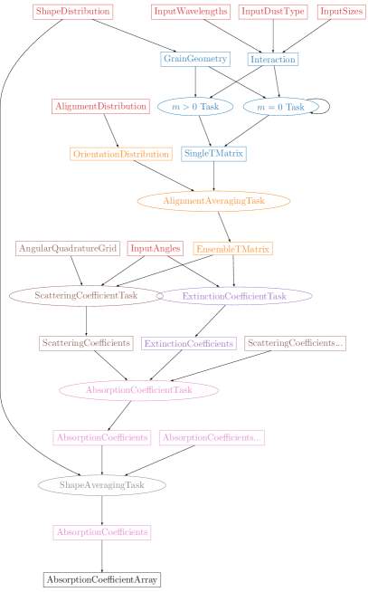
Fig. 19 shows the dependency graph for the calculation of an absorption coefficient table like the one presented in Section 3. This dependency graph is executed in parallel using a task-based parallelisation algorithm. Details of this algorithm and its performance are presented in Appendix C. From bottom to top, the calculation of a single set of absorption coefficients for a given grain size and dust type, shape distribution, alignment distribution, incoming photon wavelength and grid of input zenith angles, involves the following steps (the colors in between brackets match the colors in the flowchart):

Shape averaging (gray)

The calculation of a single set of absorption coefficients requires the calculation of the shape distribution average for absorption coefficients with the same grain size and type, alignment distribution, incoming wavelength and zenith angle grid. At the start of the calculation, a set of representative shapes is generated. For each shape, a full set of absorption coefficients is computed. Once all of these are available, they are combined into a single average set of coefficients.

Absorption coefficient calculation (pink)

A single set of absorption coefficients is calculated by taking the extinction coefficients for the same input parameters and correcting for the scattering contribution for the same parameters over a representative grid of quadrature angles according to equation (6).

Exinction coefficients (purple)

The extinction coefficients are calculated from equations (26)-(32) for the given grid of input angles and using the alignment averaged ensemble T-matrix for the given grain size, dust type, alignment distribution and incoming wavelength. We only compute the elements of the extinction matrix that are required in the end result.

Scattering coefficients (brown)

The scattering coefficients are similarly calculated from equations (10)-(25), again only computing the elements that we need. The numerical quadrature of the scattering correction term requires a grid of quadrature angles; the resolution of this grid (and hence the accuracy of the correction) is also an input parameter (see Section 2.2).

Ensemble T-matrix (orange)

The T-matrix for a given interaction is the result of ensemble-averaging the T-matrix for a single grain over the orientation distribution that is determined by the given alignment distribution and grain size. The unaveraged T-matrix still depends on the given input grain size, grain type and incoming photon wavelength.

Single T-matrix (blue)

The calculation of an individual T-matrix requires an iterative procedure whereby the order of the spherical basis function expansion is iteratively increased until the resulting T-matrix is sufficiently converged. To speed up this process, the procedure is performed using a reduced version of the T-matrix ($m=0$ tasks). Once convergence is reached, the missing components of the T-matrix can be computed ($m>0$ tasks); the latter computation can be done in parallel for different values of the expansion order $m$. The T-matrix calculation depends on two sets of input parameters: the dust grain geometry which only depends on the shape (and hence the input shape distribution), and the interaction parameters – the input wavelength, grain size and dust type, which together also determine the refractive index.

4.2 Python module

CosTuuM itself has a relatively small set of functionalities, but its results could conceivable be used in many different ways. This makes it an ideal target to be turned into a Python library. In our design, the entire calculation outlined in Section 4.1 is contained within a single library function that reads input parameters from NumPy arrays. The result of the calculation is also returned in NumPy array format. This makes it possible to incorporate the CosTuuM calculation within a script that directly manipulates the output in any conceivable manner.

We aimed to make CosTuuM both easy to use for non expert users and highly flexible for more experienced users. For this reason, most program components (e.g. the shape distribution, the material properties…) are exposed as separate Python objects, with specific customizable implementations that use user-provided functions (e.g. a user-provided function that returns the refractive index for a dust grain with given properties). These classes are hidden by sensible defaults from users that are not as familiar with the way the library works.

All of the figures in this work (except for Fig. 1) where generated using the CosTuuM Python library and are included within the public repository for the code. Potential users are encouraged to use these scripts as a reference when creating their own CosTuuM based scripts.

5 Conclusion

In this work, we presented the open-source software package CosTuuM that can be used to compute absorption and emission coefficients for arbitrary mixtures of spheroidal dust grains that are (partially) aligned with a magnetic field. We showed that CosTuuM reproduces widely used results from literature, and that is fit for its purpose: providing accurate optical properties for use in radiative transfer applications. We emphasized this point by predicting the expected polarization signal for perfectly aligned silicate grains at the wavelengths for the B-BOP polarimeter aboard the proposed ESA/JAXA mission SPICA.

We used CosTuuM to test the validity of some common approximations. We first looked at the absorption cross sections and linear polarization fraction for an ensemble of dust grains that all have the same shape and size, and that are aligned with a magnetic field according to a known alignment distribution. We find that the absorption coefficients and linear polarization function computed using CosTuuM can be accurately reproduced using a mixture of randomly oriented and perfectly aligned grains, and that both techniques are more accurate at short wavelengths than the widely used picket fence alignment approximation. This finding is important for applications where grain alignment depends on spatial position, since it makes it possible to obtain all properties using a combination of just two pre-computed tables, provided that an appropriate polarized fraction can be defined.

Next, we compared the absorption cross section and linear polarization fraction as a function of zenith angle for different grain shape distributions, and assuming an ensemble of grains with a realistic size distribution. We find that a realistic grain shape distribution consisting of both oblate and prolate grains has a similar zenith angle dependence for both quantities as a representative oblate grain with a fixed shape. We however also find that it is not possible to represent both quantities simultaneously with a single representative grain. While the ensemble average absorption coefficient for the mixture is similar to that of oblate grains with relatively large axis ratios $d>2$, the matching linear polarization fraction is more similar to oblate grains with moderate axis ratios ($d\approx{}1.6$). The discrepancies we find between various single shape approximations are much more significant than the differences between self-consistent alignment and picket fence alignment. Insufficient knowledge of an appropriate shape distribution is hence the main obstacle in obtaining accurate optical properties.

Appendix A T-matrix calculation

A.1 The T-matrix

The T-matrix method was first introduced by Waterman (1971) and consequently adopted by Tsang et al. (1981); Mishchenko & Travis (1998) and others, see Doicu et al. (2018) for a recent derivation. Below, we give a practical summary of the method as we have implemented it in CosTuuM.

The calculation of the T-matrix for a single scatterer is based on an expansion of the incoming, local and scattered electromagnetic waves in spherical basis functions. These basis functions are the general solutions of the Helmholtz equation

$$\nabla{}^{2}\boldsymbol{A}+k^{2}\boldsymbol{A}=0$$ (A1)

in spherical coordinates, and are given by

$$\boldsymbol{M}_{mn}(r,\theta{},\phi{}) =\nabla{}\times{}\boldsymbol{A}_{mn}(r,\theta{},\phi{}),$$ (A2)

$$\boldsymbol{N}_{mn}(r,\theta{},\phi{}) =\frac{1}{k}\nabla{}\times{}\left(\nabla{}\times{}\boldsymbol{A}_{mn}(r,\theta{},\phi{})\right),$$ (A3)

$${\rm{}Rg}\boldsymbol{M}_{mn}(r,\theta{},\phi{}) =\nabla{}\times{}{\rm{}Rg}\boldsymbol{A}_{mn}(r,\theta{},\phi{}),$$ (A4)

$${\rm{}Rg}\boldsymbol{N}_{mn}(r,\theta{},\phi{}) =\frac{1}{k}\nabla{}\times{}\left(\nabla{}\times{}{\rm{}Rg}\boldsymbol{A}_{mn}(r,\theta{},\phi{})\right),$$ (A5)

with

$$\boldsymbol{A}_{mn}(r,\theta{},\phi{}) =B_{mn}(\theta{},\phi{})h^{(1)}_{n}(kr)\boldsymbol{r},$$ (A6)

$${\rm{}Rg}\boldsymbol{A}_{mn}(r,\theta{},\phi{}) =B_{mn}(\theta{},\phi{})j^{(1)}_{n}(kr)\boldsymbol{r}$$ (A7)

and

$$B_{mn}(\theta{},\phi{})=(-1)^{m}\frac{1}{\sqrt{4\pi{}}}\sqrt{\frac{2n+1}{n(n+1)}}{\rm{}e}^{im\phi{}}d^{n}_{0m}(\theta{}).$$ (A8)

In these expressions, the radial dependence is given by the spherical Hankel and Bessel functions of the first kind, $h^{(1)}_{n}(x)$ and $j^{(1)}_{n}(x)$, while the dependence on the zenith angle $\theta{}$ is given by the Wigner d-functions

$$d^{n}_{0m}(\theta{})=(-1)^{m}\sqrt{\frac{(n-m)!}{(n+m)!}}P^{m}_{n}(\cos\theta{}),$$ (A9)

with $P^{m}_{n}(x)$ the associated Legendre polynomial of degree $n$ and order $m$. The expansion in theory goes up to $n=\infty{}$, but in practice can usually be truncated at some finite $n_{\rm{}max}$. The order $m$ in these expressions has values $m\in{}[-n,n]$.

Note that the basis functions $[\boldsymbol{M},\boldsymbol{N}]_{mn}$ and their regular (${\rm{}Rg}$) counterparts satisfy the following relations:

$$\frac{1}{k}\nabla{}\times{}\boldsymbol{N}_{mn} =\boldsymbol{M}_{mn},$$ (A10)

$$\frac{1}{k}\nabla{}\times{}\boldsymbol{M}_{mn} =\boldsymbol{N}_{mn},$$ (A11)

which can be easily verified using the generating Helmholtz equation.

To calculate the T-matrix, the incoming (plane) electromagnetic wave is expanded in terms of the spherical basis functions ${\rm{}Rg}[\boldsymbol{M},\boldsymbol{N}]_{mn}(kr,\theta{},\phi{})$, while the scattered (spherical) wave is expanded in terms of the $[\boldsymbol{M},\boldsymbol{N}]_{mn}(kr,\theta{},\phi{})$. The T-matrix or transition matrix is the matrix that links the expansion coefficients in both expansions. Following Waterman (1971), we can obtain the T-matrix by requiring that the tangential components of the electromagnetic field are continuous across the boundaries between the vacuum and the scattering particle. To this end, we also need the expansion of the internal electromagnetic field in terms of ${\rm{}Rg}[\boldsymbol{M},\boldsymbol{N}]_{mn}(k_{r}r,\theta{},\phi{})$, where $k_{r}=km_{r}$ is now a generalized wavenumber that also includes the (complex) refractive index of the scattering particle, $m_{r}$.

Within this so called extended boundary condition framework, the T-matrix is given by

$$\mathbf{T}=-{\rm{}Rg}\mathbf{Q}\mathbf{Q}^{-1},$$ (A12)

where the matrix $Q$ is given by

$$\mathbf{Q}=\begin{pmatrix}\mathbf{Q}^{MM}&\mathbf{Q}^{MN}\\ \mathbf{Q}^{NM}&\mathbf{Q}^{NN}\end{pmatrix},$$ (A13)

with

$$Q^{XY}_{mnm^{\prime}n^{\prime}}=k\int{}{\rm{}d}\boldsymbol{\sigma{}}.\left[\right.\\ \left.\left(\nabla{}\times{}{\rm{}Rg}\boldsymbol{X}_{m^{\prime}n^{\prime}}(k_{r}r,\theta{},\phi{})\right)\times{}\boldsymbol{Y}_{mn}(kr,\theta{},\phi{})\right.\\ \left.+{\rm{}Rg}\boldsymbol{X}_{m^{\prime}n^{\prime}}(k_{r}r,\theta{},\phi{})\times{}\left(\nabla{}\times{}\boldsymbol{Y}_{mn}(kr,\theta{},\phi{})\right)\right],$$ (A14)

with the surface element in this expression given by

$${\rm{}d}\boldsymbol{\sigma{}}=r^{2}\sin\theta{}{\rm{}d}\theta{}{\rm{}d}\phi{}\left(\hat{r}-\frac{1}{r}\frac{{\rm{}d}r(\theta{})}{{\rm{}d}\theta{}}\hat{\theta{}}\right),$$ (A15)

where $\hat{r}$ and $\hat{\theta{}}$ represent the radial and zenithal unit vectors in the spherical coordinate system, and $r(\theta{})$ is the equation that describes the surface of the spheroid. To get the regular matrix ${\rm{}Rg}\mathbf{Q}$, it suffices to replace the non-regular basis functions with their regular counterparts in these expressions.

The full expressions for the matrix elements $Q^{XY}$ can be derived by substituting the expressions for the basis functions in equation (A14) and carrying out the trivial integration over the azimuthal angle $\phi{}$:

$$\int_{0}^{2\pi{}}{\rm{}e}^{i(m-m^{\prime})\phi{}}{\rm{}d}\phi{}=2\pi{}\delta{}_{mm^{\prime}},$$ (A16)

with $\delta{}_{mm^{\prime}}$ the Kronecker delta. We can precompute (based on Tsang et al., 1981)

$$(MM)_{m_{1}n_{1}m_{2}n_{2}}=\\ \begin{gathered}\int{}{\rm{}d}\boldsymbol{\sigma{}}.\left[\boldsymbol{M}_{m_{1}n_{1}}(k_{1}r,\theta{},\phi{})\times{}\boldsymbol{M}_{m_{2}n_{2}}(k_{2}r,\theta{},\phi{})\right]=\\ -\frac{i}{2}C_{n_{1}n_{2}}(-1)^{m_{1}+m_{2}}\delta{}_{m_{1}-m_{2}}\\ \int_{0}^{\pi{}}r^{2}\sin\theta{}h^{(1)}_{n_{1}}(k_{1}r)h^{(1)}_{n_{2}}(k_{2}r)\\ \left[\pi{}_{m_{1}n_{1}}(\theta{})\tau{}_{-m_{1}n_{2}}(\theta{})\right.\\ \left.-\tau{}_{m_{1}n_{1}}(\theta{})\pi{}_{-m_{1}n_{2}}(\theta{})\right]{\rm{}d}\theta{},\end{gathered}$$ (A17)

$$(MN)_{m_{1}n_{1}m_{2}n_{2}}=\\ \begin{gathered}\int{}{\rm{}d}\boldsymbol{\sigma{}}.\left[\boldsymbol{M}_{m_{1}n_{1}}(k_{1}r,\theta{},\phi{})\times{}\boldsymbol{N}_{m_{2}n_{2}}(k_{2}r,\theta{},\phi{})\right]=\\ \frac{1}{2}C_{n_{1}n_{2}}(-1)^{m_{1}+m_{2}}\delta{}_{m_{1}-m_{2}}\\ \int_{0}^{\pi{}}r^{2}\sin\theta{}\Bigg{(}h^{(1)}_{n_{1}}(k_{1}r){\rm{}D}h^{(1)}_{n_{2}}(k_{2}r)\\ \left[-\pi{}_{m_{1}n_{1}}(\theta{})\pi{}_{-m_{1}n_{2}}(\theta{})+\tau{}_{m_{1}n_{1}}(\theta{})\tau{}_{-m_{1}n_{2}}(\theta{})\right]\\ +\frac{1}{r}\frac{{\rm{}d}r(\theta{})}{{\rm{}d}\theta{}}\frac{n_{2}(n_{2}+1)}{k_{2}r}\\ h^{(1)}_{n_{1}}(k_{1}r)h^{(1)}_{n_{2}}(k_{2}r)\tau{}_{m_{1}n_{1}}(\theta{})d^{n_{2}}_{0-m_{1}}(\theta{})\Bigg{)}{\rm{}d}\theta{}\\ =-\int{}{\rm{}d}\boldsymbol{\sigma{}}.\left[\boldsymbol{N}_{m_{2}n_{2}}(k_{2}r,\theta{},\phi{})\times{}\boldsymbol{M}_{m_{1}n_{1}}(k_{1}r,\theta{},\phi{})\right]\end{gathered}\\ =-(NM)_{m_{2}n_{2}m_{1}n_{1}},$$ (A18)

$$(NN)_{m_{1}n_{1}m_{2}n_{2}}=\\ \begin{gathered}\int{}{\rm{}d}\boldsymbol{\sigma{}}.\left[\boldsymbol{N}_{m_{1}n_{1}}(k_{1}r,\theta{},\phi{})\times{}\boldsymbol{N}_{m_{2}n_{2}}(k_{2}r,\theta{},\phi{})\right]=\\ -\frac{i}{2}C_{n_{1}n_{2}}(-1)^{m_{1}+m_{2}}\delta{}_{m_{1}-m_{2}}\\ \int_{0}^{\pi{}}r^{2}\sin\theta{}\Big{(}{\rm{}D}h^{(1)}_{n_{1}}(k_{1}r){\rm{}D}h^{(1)}_{n_{2}}(k_{2}r)\\ \left[-\tau{}_{m_{1}n_{1}}(\theta{})\pi{}_{-m_{1}n_{2}}(\theta{})+\pi{}_{m_{1}n_{1}}(\theta{})\tau{}_{-m_{1}n_{2}}(\theta{})\right]\\ +\frac{1}{r}\frac{{\rm{}d}r(\theta{})}{{\rm{}d}\theta{}}\Big{[}\frac{n_{2}(n_{2}+1)}{k_{2}r}{\rm{}D}h^{(1)}_{n_{1}}(k_{1}r)h^{(1)}_{n_{2}}(k_{2}r)\\ \pi{}_{m_{1}n_{1}}(\theta{})d^{n_{2}}_{0-m_{1}}(\theta{})-\\ \frac{n_{1}(n_{1}+1)}{k_{1}r}h^{(1)}_{n_{1}}(k_{1}r){\rm{}D}h^{(1)}_{n_{2}}(k_{2}r)\\ d^{n_{1}}_{0m_{1}}(\theta{})\pi{}_{-m_{1}n_{2}}(\theta{})\Big{]}\Bigg{)}{\rm{}d}\theta{},\end{gathered}$$ (A19)

with

$$C_{nn^{\prime}} =\sqrt{\frac{(2n+1)(2n^{\prime}+1)}{n(n+1)n^{\prime}(n^{\prime}+1)}},$$ (A20)

$$\pi{}_{mn}(\theta{}) =\frac{m}{\sin(\theta{})}d^{n}_{0m}(\theta{}),$$ (A21)

$$\tau{}_{mn}(\theta{}) =\frac{d}{d\theta{}}d^{n}_{0m}(\theta{}),$$ (A22)

$${\rm{}D}h^{(1)}_{n}(x) =\frac{[xh^{(1)}_{n}(x)]^{\prime}}{x}=\frac{{\rm{}d}}{{\rm{}d}x}h^{(1)}_{n}(x)-\frac{1}{x}h^{(1)}_{n}(x).$$ (A23)

In these expressions, the spherical Hankel functions $h^{(1)}_{n}(x)$ are to be replaced with the corresponding spherical Bessel functions $j^{(1)}_{n}(x)$ where appropriate when substituting ${\rm{}Rg}[M,N]$ for $[M,N]$.

To carry out the second integration over the zenith angle $\theta{}$, we follow Tsang et al. (1981); Mishchenko & Travis (1998) and use a numerical Gauss-Legendre quadrature in the variable $\cos(\theta{})$. Note that to derive the expressions above, we have made use of the relation

$$d^{n}_{0m}(\theta{})=(-1)^{m}d^{n}_{0-m}(\theta{})$$ (A24)

and its derivative.

The final expressions for the elements of the matrix $\mathbf{Q}$ are then

$$Q^{MM}_{mnm^{\prime}n^{\prime}} =kk_{r}({\rm{}Rg}NM)_{mnm^{\prime}n^{\prime}}+k^{2}({\rm{}Rg}MN)_{mnm^{\prime}n^{\prime}},$$ (A25)

$$Q^{MN}_{mnm^{\prime}n^{\prime}} =kk_{r}({\rm{}Rg}MM)_{mnm^{\prime}n^{\prime}}+k^{2}({\rm{}Rg}NN)_{mnm^{\prime}n^{\prime}},$$ (A26)

$$Q^{NM}_{mnm^{\prime}n^{\prime}} =kk_{r}({\rm{}Rg}NN)_{mnm^{\prime}n^{\prime}}+k^{2}({\rm{}Rg}MM)_{mnm^{\prime}n^{\prime}},$$ (A27)

$$Q^{NN}_{mnm^{\prime}n^{\prime}} =kk_{r}({\rm{}Rg}MN)_{mnm^{\prime}n^{\prime}}+k^{2}({\rm{}Rg}NM)_{mnm^{\prime}n^{\prime}}.$$ (A28)

The T-matrix for a spheroid in a reference frame where the vertical axis is aligned with the rotation axis of the spheroid has a number of properties, including

$$T^{(ij)}_{mnm^{\prime}n^{\prime}} =\delta{}_{mm^{\prime}}T^{(ij)}_{mnmn^{\prime}}$$ (A29)

$$T^{(ij)}_{mnmn^{\prime}} =T^{(ji)}_{-mn-mn^{\prime}}=(-1)^{i+j}T^{(ij)}_{-mn-mn^{\prime}},$$ (A30)

where $i=1,2$ and $j=1,2$ represent the $\boldsymbol{M}$ and $\boldsymbol{N}$ blocks in the T-matrix respectively. The former relation means that the T-matrix is a block diagonal matrix in the index $m$, which allows us to compute it separately for different values of $m$, while the latter relation means we only need to compute the matrix elements for positive values of $m$. As in Mishchenko & Travis (1998), this leads to the following general approach to computing the T-matrix for a single spheroidal particle:

1. Compute the $m=0$ component of the T-matrix for a suitable guess of $n_{\rm{}max}$ and the number of Gauss-Legendre quadrature points $n_{\rm{}GL}$. Compute the average extinction and scattering cross sections for randomly oriented grains (Mishchenko & Travis, 1998)

   $$\langle{}C_{\rm{}ext}\rangle{} =-\frac{2\pi{}}{k^{2}}\sum_{n=1}^{n_{\rm{}max}}\sum_{m=-n}^{n}\sum_{i=1}^{2}{\rm{}Re}\left(T^{(ii)}_{mnmn}\right),$$ (A31)

   $$\langle{}C_{\rm{}sca}\rangle{} =\frac{2\pi{}}{k^{2}}\sum_{n=1}^{n_{\rm{}max}}\sum_{n^{\prime}=1}^{n_{\rm{}max}}\sum_{m=-n}^{n}\sum_{m^{\prime}=-n^{\prime}}^{n^{\prime}}\sum_{i=1}^{2}\sum_{j=1}^{2}\left|T^{(ij)}_{mnm^{\prime}n^{\prime}}\right|^{2}$$ (A32)

   for this sparse version of the T-matrix, where ${\rm{}Re}(z)$ represents the real part of the complex number $z$, while $|z|^{2}=zz^{*}$ is its norm. Repeat this for $n^{\prime}_{\rm{}max}=n_{\rm{}max}+1$ until the relative difference between the respective values for $\langle{}C_{\rm{}ext}\rangle{}$ and $\langle{}C_{\rm{}sca}\rangle{}$ for two successive $n_{\rm{}max}$ values drops below some desired tolerance, $\tau{}$ (we use $\tau{}=10^{-4}$). This determines $n_{\rm{}max}$.

2. Now increase the number of Gauss-Legendre quadrature points $n^{\prime}_{\rm{}GL}=n_{\rm{}GL}+1$ and repeat this until the relative differences for $\langle{}C_{\rm{}ext}\rangle{}$ and $\langle{}C_{\rm{}sca}\rangle{}$ again drop below $\tau{}$. This determines $n_{\rm{}GL}$. Note that we generally do not perform this step in CosTuuM because it makes it harder to efficiently parallelize the algorithm. Instead, we assume a fixed ratio $n_{\rm{}max}/n_{\rm{}GL}=2$, which converges for all our tests.

3. Now use these values of $n_{\rm{}max}$ and $n_{\rm{}GL}$ to compute the additional T-matrix elements for $m>0$. The elements for $m<0$ can be found using equation (A30) and are not used in further calculations for that same reason.

A.2 Orientational averages

As shown in Mishchenko (1991), it is possible to compute the T-matrix for an ensemble of spheroidal grains with different orientations w.r.t. a reference axis. Given the orientation distribution for the ensemble of grains (normalized according to equation (33)), tke T-matrix for the ensemble can be computed as

$$\langle{}T^{(ij)}_{mnmn^{\prime}}\rangle{}=\sum_{m_{1}=-{\rm{}min}(n,n^{\prime})}^{{\rm{}min}(n,n^{\prime})}\sum_{n_{1}=|n-n^{\prime}|}^{n+n^{\prime}}\\ (-1)^{m+m_{1}}p_{n_{1}}C^{n_{1}0}_{nmn^{\prime}-m}C^{n_{1}0}_{nm_{1}n^{\prime}-m_{1}}T^{(ij)}_{m_{1}nm_{1}n^{\prime}},$$ (A33)

where $C^{NM}_{n_{1}m_{1}n_{2}m_{2}}$ are the Clebsch-Gordan coefficients and

$$p_{n}=\int_{0}^{\pi{}}p(\beta{})d^{n}_{00}(\beta{})\sin\beta{}{\rm{}d}\beta{}$$ (A34)

are the coefficients of the expansion of the orientation distribution in Legendre polynomials.

Due to the orthogonality of the Legendre polynomials, the normalization condition (33) can be guaranteed by setting $p_{0}=1$. The Mishchenko distribution used in Section 3.1 can be recovered by setting all coefficients other than $p_{0}$ and $p_{2}$ to 0.

A.3 Parity rules

The calculation of the T-matrix elements can be significantly simplified by taking into account the following parity rules:

$$d^{n}_{0m}(\pi{}-\theta{}) =(-1)^{n+m}d^{n}_{0m}(\theta{}),$$ (A35)

$$\pi{}_{mn}(\pi{}-\theta{}) =(-1)^{n+m}d^{n}_{0m}(\theta{}),$$ (A36)

$$\tau_{mn}(\pi{}-\theta{}) =(-1)^{n+m+1}\tau{}_{mn}(\theta{}),$$ (A37)

which can all be derived from the parity rule for the associated Legendre polynomials:

$$P^{m}_{n}(-x)=(-1)^{n+m}P^{m}_{n}(x).$$ (A38)

Over the integration interval $[0,\pi{}]$, this means that the $(MN)_{m_{1}n_{1}m_{2}n_{2}}$ elements are only non-zero for even values of $n_{1}+n_{2}$, while the $(MM)_{m_{1}n_{1}m_{2}n_{2}}$ and $(NN)_{m_{1}n_{1}m_{2}n_{2}}$ elements are only non-zero for odd values. Both of these results are irrespective of the values of $m_{1}$ and $m_{2}$ because of the appearance of the Kronecker delta in the expressions for the matrix elements.

Similar rules can be derived w.r.t. the sign of $m$:

$$\pi{}_{-mn}(\theta{}) =(-1)^{m+1}\pi{}_{mn}(\theta{}),$$ (A39)

$$\tau{}_{-mn}(\theta{}) =(-1)^{m}\tau{}_{mn}(\theta{}).$$ (A40)

These will prove useful below.

Appendix B Scattering events

B.1 The forward scattering matrix

In a reference frame where the rotation axis of the spheroidal particle is aligned with the vertical axis, the $\mathbf{S}$ matrix can be computed using (Mishchenko, 2000)

$$\begin{gathered}S_{\theta{}\theta{}}=\frac{1}{k}\sum_{n=1}^{n_{max}}\sum_{n^{\prime}=1}^{n_{max}}\sum_{m=-\min(n,n^{\prime})}^{\min(n,n^{\prime})}C^{\prime}_{nn^{\prime}}{\rm{}e}^{im(\phi{}_{s}^{P}-\phi{}_{i}^{P})}\Big{[}\\ T^{11}_{mnmn^{\prime}}\pi{}_{mn}(\theta{}_{s}^{P})\pi{}_{mn^{\prime}}(\theta{}_{i}^{P})\\ +T^{21}_{mnmn^{\prime}}\tau{}_{mn}(\theta{}_{s}^{P})\pi{}_{mn^{\prime}}(\theta{}_{i}^{P})\\ +T^{12}_{mnmn^{\prime}}\pi{}_{mn}(\theta{}_{s}^{P})\tau{}_{mn^{\prime}}(\theta{}_{i}^{P})\\ +T^{22}_{mnmn^{\prime}}\tau{}_{mn}(\theta{}_{s}^{P})\tau{}_{mn^{\prime}}(\theta{}_{i}^{P})\Big{]},\end{gathered}$$ (B1)

$$\begin{gathered}S_{\theta{}\phi{}}=-\frac{i}{k}\sum_{n=1}^{n_{max}}\sum_{n^{\prime}=1}^{n_{max}}\sum_{m=-\min(n,n^{\prime})}^{\min(n,n^{\prime})}C^{\prime}_{nn^{\prime}}{\rm{}e}^{im(\phi{}_{s}^{P}-\phi{}_{i}^{P})}\Big{[}\\ T^{11}_{mnmn^{\prime}}\pi{}_{mn}(\theta{}_{s}^{P})\tau{}_{mn^{\prime}}(\theta{}_{i}^{P})\\ +T^{21}_{mnmn^{\prime}}\tau{}_{mn}(\theta{}_{s}^{P})\tau{}_{mn^{\prime}}(\theta{}_{i}^{P})\\ +T^{12}_{mnmn^{\prime}}\pi{}_{mn}(\theta{}_{s}^{P})\pi{}_{mn^{\prime}}(\theta{}_{i}^{P})\\ +T^{22}_{mnmn^{\prime}}\tau{}_{mn}(\theta{}_{s}^{P})\pi{}_{mn^{\prime}}(\theta{}_{i}^{P})\Big{]},\end{gathered}$$ (B2)

$$\begin{gathered}S_{\phi{}\theta{}}=\frac{i}{k}\sum_{n=1}^{n_{max}}\sum_{n^{\prime}=1}^{n_{max}}\sum_{m=-\min(n,n^{\prime})}^{\min(n,n^{\prime})}C^{\prime}_{nn^{\prime}}{\rm{}e}^{im(\phi{}_{s}^{P}-\phi{}_{i}^{P})}\Big{[}\\ T^{11}_{mnmn^{\prime}}\tau{}_{mn}(\theta{}_{s}^{P})\pi{}_{mn^{\prime}}(\theta{}_{i}^{P})\\ +T^{21}_{mnmn^{\prime}}\pi{}_{mn}(\theta{}_{s}^{P})\pi{}_{mn^{\prime}}(\theta{}_{i}^{P})\\ +T^{12}_{mnmn^{\prime}}\tau{}_{mn}(\theta{}_{s}^{P})\tau{}_{mn^{\prime}}(\theta{}_{i}^{P})\\ +T^{22}_{mnmn^{\prime}}\pi{}_{mn}(\theta{}_{s}^{P})\tau{}_{mn^{\prime}}(\theta{}_{i}^{P})\Big{]},\end{gathered}$$ (B3)

$$\begin{gathered}S_{\phi{}\phi{}}=\frac{1}{k}\sum_{n=1}^{n_{max}}\sum_{n^{\prime}=1}^{n_{max}}\sum_{m=-\min(n,n^{\prime})}^{\min(n,n^{\prime})}C^{\prime}_{nn^{\prime}}{\rm{}e}^{im(\phi{}_{s}^{P}-\phi{}_{i}^{P})}\Big{[}\\ T^{11}_{mnmn^{\prime}}\tau{}_{mn}(\theta{}_{s}^{P})\tau{}_{mn^{\prime}}(\theta{}_{i}^{P})\\ +T^{21}_{mnmn^{\prime}}\pi{}_{mn}(\theta{}_{s}^{P})\tau{}_{mn^{\prime}}(\theta{}_{i}^{P})\\ +T^{12}_{mnmn^{\prime}}\tau{}_{mn}(\theta{}_{s}^{P})\pi{}_{mn^{\prime}}(\theta{}_{i}^{P})\\ +T^{22}_{mnmn^{\prime}}\pi{}_{mn}(\theta{}_{s}^{P})\pi{}_{mn^{\prime}}(\theta{}_{i}^{P})\Big{]},\end{gathered}$$ (B4)

with

$$C^{\prime}_{nn^{\prime}}=i^{n^{\prime}-n-1}C_{nn^{\prime}}=i^{n^{\prime}-n-1}\sqrt{\frac{(2n+1)(2n^{\prime}+1)}{n(n+1)n^{\prime}(n^{\prime}+1)}},$$ (B5)

and $\pi{}_{mn}(\theta{})$ and $\tau{}_{mn}(\theta{})$ as given in equations (A21) and (A22).

Using the symmetry relations for the T-matrix and the rules given above, it can be shown that the expressions in between brackets for $S_{\theta{}\theta{}}$ and $S_{\phi{}\phi{}}$ are even under a $m\rightarrow{}-m$ substitution, while the expressions in between brackets for $S_{\theta{}\phi{}}$ and $S_{\phi{}\theta{}}$ are odd. Combined with the respective odd and even nature of the real and imaginary parts of $e^{im(\phi{}_{s}^{P}-\phi{}_{i}^{P})}=\cos\left(m(\phi{}_{s}^{P}-\phi{}_{i}^{P})\right)+i\sin\left(m(\phi{}_{s}^{P}-\phi{}_{i}^{P})\right)$, this allows us to significantly simplify the calculation of the forward scattering matrix elements. By rearranging the equations further so that the sum over $m$ becomes the outer loop, we can additionally compute the exponential factor recursively, so that only two (expensive) evaluations of trigonometric functions are required per scattering interaction.

B.2 Sampling grid

When CosTuuM is used to generate tables containing absorption coefficients, these coefficients are computed on a regular angular grid in $\theta{}_{i}$. Because of the azimuthal symmetry of spheroidal grains, an arbitrary input zenith angle can be used, we choose $\phi{}_{i}=0$. To correct for the scattering contribution, we need to subtract the relevant scattering matrix components, integrated over all incoming scattering angles. We will use a 2D grid of Gauss-Legendre quadrature points in $\phi{},\cos\theta{}$ for this.

In the end, we are hence left with a small grid of angles that are known at the start of the computation. As an optimization, we can precompute the trigonometric functions and related functions (i.e. the Wigner d-functions and derivatives) on this grid, and use grid indices rather than angles to obtain the relevant function values when needed. Surprisingly, this approach does not result in a significant speed gain on our test systems, indicating that memory bandwidth issues rather than processor speed are determining the overall cost of the algorithm.

Appendix C Task-based parallelisation

C.1 Algorithm

The overall structure of the T-matrix algorithm (as illustrated in Fig. 19) makes this algorithm perfectly suited for a task-based parallelisation strategy (Gonnet et al., 2016), a parallel programming paradigm that has gained recent interest in the astrophysical simulation community (Bordner & Norman, 2012; Schaller et al., 2016; White et al., 2016; Nordlund et al., 2018). Within this paradigm, the entire calculation is broken down into small chunks (tasks) that can be executed concurrently. These tasks act on resources, i.e. structured memory blocks that contain intermediate results and are stored in a large shared memory pool. Tasks that require access to the same resource cannot be executed simultaneously by different threads, while tasks that depend on the result of another task need to be executed after that other task finishes. These dependencies can be derived from the dependency graph in Fig. 19.

Some components required by the calculation outlined in Fig. 19 can be reused between tasks. If for example two values for one of the input parameters (e.g. the grain size) are given, then the shape averaging procedure has to be done twice: once for every value of the grain size. The quadrature points used to sample the shape distribution can in this case be reused and the dust grain geometries, which only depend on these quadrature points, only need to be computed once. Similarly, the quadrature grid used to compute the scattering correction can be shared between all scattering coefficient calculations. The calculation of a single T-matrix contains a number of precomputed special functions that are not shown in Fig. 19 and that can also be reused.

Creating all the tasks and resources required to execute Fig. 19 and making sure that resources are optimally shared between tasks is a complex bookkeeping exercise that can be executed very efficiently. Once the tasks and the graph of task and resource dependencies are constructed, we pass them on to the QuickSched library (Gonnet et al., 2016) that takes care of the parallel execution of the graph.

The various resources involved in the calculations need to be stored in memory. In order to avoid expensive memory allocations that could lead to severe bottlenecks during parallel execution, we preallocate all required memory during task construction. Some of the components (e.g. the spherical Bessel functions required for the T-matrix calculation and the T-matrices themselves) have large sizes, which makes it impractical to allocate a unique memory block for each of them within the memory limits of a modern system. We therefore limit the total number of these blocks and reuse blocks that are no longer used. This is only possible if we add additional dependencies between tasks that ensure a memory block can only be reused if the previous tasks that depended on its old state have finished, which further complicates the bookkeeping.

In the end, the total allowed memory usage of CosTuuM is treated as an input parameter. If the allowed memory size is insufficient to fit the resources required for a single ensemble T-matrix calculation, the calculation will abort. The minimum required size depends on the maximum allowed spherical basis function expansion in the T-matrix calculation and the requested accuracy, but is typically of the order of $1-10$ GB.

Figure 20: Task plot for a small CosTuuM calculation using 8 computing threads. The different colors correspond to the different steps in Fig. 19, as indicated in the legend. Some steps are not visible because their contribution is too small; they have been omitted from the legend. Different opacity values within the same color correspond to different subtasks within a step. The green bars correspond to technical tasks required to handle the reuse of resources.

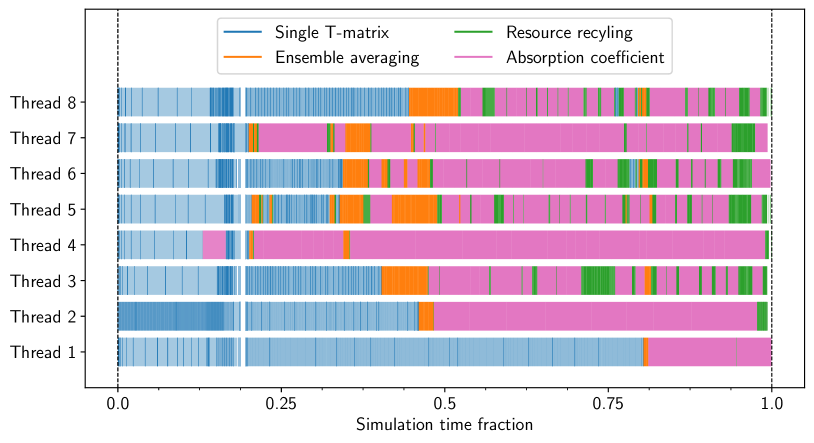
The QuickSched library internally stores hardware counters that measure the elapsed CPU time for each task during execution. This makes it possible to generate detailed diagnostic task plots that show how each parallel thread involved in the computation performs over time. Fig. 20 shows an example of a task plot generated by one of our parallel runs. As can be seen, the execution of the tasks happens stochastically and unsynchronized, with different threads executing different tasks at the same time according to what is available. Overall, the parallel efficiency of the algorithm is good, with only small bottlenecks or load-imbalances (which show up as empty gaps in the task plot).

C.2 Performance

Figure 21: Parallel efficiency for a strong scaling test with CosTuuM as measured on two different systems using two different ways to assign parallel threads to physical cores, as indicated in the legends. The top panel shows the usual parallel efficiency computed using a single thread run as reference, the bottom panel shows the same quantity but using twice the two thread run as reference. The latter partially eliminates the effect of additional memory costs.

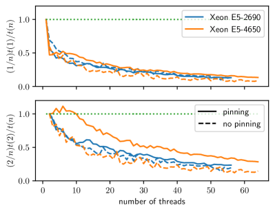
Fig. 21 shows the parallel efficiency of CosTuuM for the same run as shown in the task plot, but now for a variable number of threads. We measured performance on two different systems: a 64 core system using Intel Xeon E5-4650 CPUs, and a 56 core system using Intel Xeon E5-2690 CPUs. Both systems have a similar memory layout, but the latter system is faster due to a higher CPU clock speed and better CPU optimizations. For both systems, we ran with two different ways of assigning threads to physical cores as set by the OpenMP OMP_PROC_BIND environment variable. The default value (False) allows the kernel to run threads on the same core and move threads during the calculation, while a value of True forces threads to run on different cores and binds them to that core, this is called pinning.

On both systems, there is a significant decrease in efficiency when moving from 1 to multiple threads, and this decrease is more pronounced when pinning forces all threads to run on separate cores. This decrease is entirely due to the memory access pattern of CosTuuM: a number of tasks in the task graph make use of large blocks of continuous memory and the average execution time of these tasks increases when increasing the number of threads from 1 to 2. If we factor in the increase in memory access time by using the 2 thread run as a reference to compute the parallel efficiency, then the scaling of CosTuuM is significantly better. The slower system, which is less affected by memory bandwidth issues benefits more from this approach; this system also shows a more significant efficiency gain when threads are pinned to cores.

We conclude that the task based algorithm does lead to low load imbalances during parallel runs, but that the current memory usage of CosTuuM hampers its overall performance. Nevertheless, a parallel speedup of up to a factor 10 is achievable, even for small calculations. The memory issues we found are difficult to solve and may be addressed in future versions of the library.

References

- Andersson et al. (2015) Andersson, B.-G., Lazarian, A., & Vaillancourt, J. E. 2015, Annual Review of Astronomy and Astrophysics, 53, 501
- André et al. (2019) André, P., Hughes, A., Guillet, V., et al. 2019, PASA, 36, e029
- Baes et al. (2011) Baes, M., Verstappen, J., De Looze, I., et al. 2011, ApJS, 196, 22
- Bertrang et al. (2017) Bertrang, G. H. M., Flock, M., & Wolf, S. 2017, MNRAS, 464, L61
- Bertrang & Wolf (2017) Bertrang, G. H. M., & Wolf, S. 2017, MNRAS, 469, 2869
- Bohren & Huffman (1983) Bohren, C. F., & Huffman, D. R. 1983, Absorption and scattering of light by small particles
- Bordner & Norman (2012) Bordner, J., & Norman, M. L. 2012, in Proceedings of the Extreme Scaling Workshop, BW-XSEDE ’12 (USA: University of Illinois at Urbana-Champaign)
- Bryan et al. (2018) Bryan, S., Austermann, J., Ferrusca, D., et al. 2018, in Society of Photo-Optical Instrumentation Engineers (SPIE) Conference Series, Vol. 10708, Proc. SPIE, 107080J
- Camps & Baes (2015) Camps, P., & Baes, M. 2015, Astronomy and Computing, 9, 20
- Camps & Baes (2020) —. 2020, arXiv e-prints, arXiv:2003.00721
- Cortes et al. (2016) Cortes, P. C., Girart, J. M., Hull, C. L. H., et al. 2016, ApJ, 825, L15
- Doicu et al. (2018) Doicu, A., Eremin, Y., Efremenko, D. S., & Trautmann, T. 2018, Methods for Electromagnetic Scattering by Large Axisymmetric Particles with Extreme Geometries, ed. T. Wriedt & Y. Eremin (Cham: Springer International Publishing), 49–69
- Draine (1985) Draine, B. T. 1985, ApJS, 57, 587
- Draine & Allaf-Akbari (2006) Draine, B. T., & Allaf-Akbari, K. 2006, ApJ, 652, 1318
- Draine & Flatau (1994) Draine, B. T., & Flatau, P. J. 1994, Journal of the Optical Society of America A, 11, 1491
- Draine & Fraisse (2009) Draine, B. T., & Fraisse, A. A. 2009, ApJ, 696, 1
- Draine & Hensley (2017) Draine, B. T., & Hensley, B. S. 2017, arXiv e-prints, arXiv:1710.08968
- Draine & Lee (1984) Draine, B. T., & Lee, H. M. 1984, ApJ, 285, 89
- Draine & Malhotra (1993) Draine, B. T., & Malhotra, S. 1993, ApJ, 414, 632
- Dyck & Beichman (1974) Dyck, H. M., & Beichman, C. A. 1974, ApJ, 194, 57
- Gonnet et al. (2016) Gonnet, P., Chalk, A. B. G., & Schaller, M. 2016, arXiv e-prints, arXiv:1601.05384
- Grand et al. (2017) Grand, R. J. J., Gómez, F. A., Marinacci, F., et al. 2017, MNRAS, 467, 179
- Hennebelle (2018) Hennebelle, P. 2018, A&A, 611, A24
- Hensley et al. (2019) Hensley, B. S., Zhang, C., & Bock, J. J. 2019, ApJ, 887, 159
- Hovenier et al. (1996) Hovenier, J. W., Lumme, K., Mishchenko, M. I., et al. 1996, J. Quant. Spec. Radiat. Transf., 55, 695
- Hunter (2007) Hunter, J. D. 2007, Computing in Science Engineering, 9, 90
- Kim & Martin (1995) Kim, S.-H., & Martin, P. G. 1995, ApJ, 444, 293
- Laor & Draine (1993) Laor, A., & Draine, B. T. 1993, ApJ, 402, 441
- Lee & Draine (1985) Lee, H. M., & Draine, B. T. 1985, ApJ, 290, 211
- Leinonen (2014) Leinonen, J. 2014, Opt. Express, 22, 1655
- Lopez-Rodriguez et al. (2020) Lopez-Rodriguez, E., Dowell, C. D., Jones, T. J., et al. 2020, ApJ, 888, 66
- Mathis et al. (1977) Mathis, J. S., Rumpl, W., & Nordsieck, K. H. 1977, ApJ, 217, 425
- Matthews et al. (2009) Matthews, B. C., McPhee, C. A., Fissel, L. M., & Curran, R. L. 2009, ApJS, 182, 143
- Min et al. (2003) Min, M., Hovenier, J. W., & de Koter, A. 2003, A&A, 404, 35
- Mishchenko & Travis (1998) Mishchenko, M., & Travis, L. D. 1998, J. Quant. Spec. Radiat. Transf., 60, 309
- Mishchenko (1991) Mishchenko, M. I. 1991, ApJ, 367, 561
- Mishchenko (2000) Mishchenko, M. I. 2000, Appl. Opt., 39, 1026
- Mishchenko et al. (2000) Mishchenko, M. I., Hovenier, J. W., & Travis, L. D. 2000, Light scattering by nonspherical particles : theory, measurements, and applications
- Nelson et al. (2019) Nelson, D., Springel, V., Pillepich, A., et al. 2019, Computational Astrophysics and Cosmology, 6, 2
- Nordlund et al. (2018) Nordlund, Å., Ramsey, J. P., Popovas, A., & Küffmeier, M. 2018, MNRAS, 477, 624
- Pattle et al. (2017) Pattle, K., Ward-Thompson, D., Berry, D., et al. 2017, ApJ, 846, 122
- Peest et al. (2017) Peest, C., Camps, P., Stalevski, M., Baes, M., & Siebenmorgen, R. 2017, A&A, 601, A92
- Pelkonen et al. (2007) Pelkonen, V. M., Juvela, M., & Padoan, P. 2007, A&A, 461, 551
- Pelkonen et al. (2009) —. 2009, A&A, 502, 833
- Pillepich et al. (2019) Pillepich, A., Nelson, D., Springel, V., et al. 2019, MNRAS, 490, 3196
- Planck Collaboration et al. (2018) Planck Collaboration, Aghanim, N., Akrami, Y., et al. 2018, arXiv e-prints, arXiv:1807.06212
- Reissl et al. (2018) Reissl, S., Stutz, A. M., Brauer, R., et al. 2018, MNRAS, 481, 2507
- Reissl et al. (2016) Reissl, S., Wolf, S., & Brauer, R. 2016, A&A, 593, A87
- Roelfsema et al. (2018) Roelfsema, P. R., Shibai, H., Armus, L., et al. 2018, PASA, 35, e030
- Santos et al. (2019) Santos, F. P., Chuss, D. T., Dowell, C. D., et al. 2019, ApJ, 882, 113
- Schaller et al. (2016) Schaller, M., Gonnet, P., Chalk, A. B. G., & Draper, P. W. 2016, arXiv e-prints, arXiv:1606.02738
- Seifried et al. (2019) Seifried, D., Walch, S., Reissl, S., & Ibáñez-Mejía, J. C. 2019, MNRAS, 482, 2697
- Siebenmorgen et al. (2014) Siebenmorgen, R., Voshchinnikov, N. V., & Bagnulo, S. 2014, A&A, 561, A82
- Somerville et al. (2013) Somerville, W. R. C., Auguié, B., & Le Ru, E. C. 2013, J. Quant. Spec. Radiat. Transf., 123, 153
- Tsang et al. (1981) Tsang, L., Kubacsi, M. C., & Kong, J. A. 1981, Radio Science, 16, 321
- van der Walt et al. (2011) van der Walt, S., Colbert, S. C., & Varoquaux, G. 2011, Computing in Science Engineering, 13, 22
- Vickers & Brown (2001) Vickers, G. T., & Brown, D. J. 2001, Proceedings of the Royal Society A, 457, 283
- Virtanen et al. (2020) Virtanen, P., Gommers, R., Oliphant, T. E., et al. 2020, Nature Methods, 17, 261
- Voshchinnikov & Farafonov (1993) Voshchinnikov, N. V., & Farafonov, V. G. 1993, Ap&SS, 204, 19
- Waterman (1971) Waterman, P. C. 1971, Phys. Rev. D, 3, 825
- White et al. (2016) White, C. J., Stone, J. M., & Gammie, C. F. 2016, ApJS, 225, 22
- Wurster & Bate (2019) Wurster, J., & Bate, M. R. 2019, MNRAS, 486, 2587