Comparing Representations for Audio Synthesis Using Generative Adversarial Networks

Abstract

In this paper, we compare different audio signal representations, including the raw audio waveform and a variety of time-frequency representations, for the task of audio synthesis with Generative Adversarial Networks (GANs). We conduct the experiments on a subset of the NSynth dataset. The architecture follows the benchmark Progressive Growing Wasserstein GAN. We perform experiments both in a fully non-conditional manner as well as conditioning the network on the pitch information. We quantitatively evaluate the generated material utilizing standard metrics for assessing generative models, and compare training and sampling times. We show that complex-valued as well as the magnitude and Instantaneous Frequency of the Short-Time Fourier Transform achieve the best results, and yield fast generation and inversion times. The code for feature extraction, training and evaluating the model is available online.

I Introduction

In recent years, deep learning for audio has shifted from using hand-crafted features requiring prior knowledge, to features learned from raw audio data or mid-level representations such as the Short-Time Fourier Transform (STFT) [1]. Indeed, this has allowed us to build models requiring less prior knowledge, yet at the expense of data, computational power, and training time [2]. For example, deep autoregressive techniques working directly on raw audio [3], as well as on Mel-scaled spectrograms [4], currently yield state-of-the-art results in terms of quality. However, these models can take up to several weeks to train in a conventional GPU, and also, their generation procedure is too slow for typical production environments. On the other hand, Generative Adversarial Networks (GANs) [5], have achieved comparable audio synthesis quality and faster generation time [6], although they still require long training times and large-scale datasets when modeling low or mid-level feature representations [7, 8].

It is still subject to debate what the best audio representations are in machine learning in general, and the best choice may also depend on the respective application and the models employed. In audio synthesis with GANs, different representations may result in different training and generation times, and may also influence the quality of the resulting output. For example, operating on representations that compress the information with respect to perceptual principles, or are structured to better support a specific model architecture, may yield faster training and generation times, but may result in worse audio quality. Therefore, in this paper, we compare different audio signal representations, including the raw audio waveform and a variety of time-frequency representations, for the task of adversarial audio synthesis with GANs. To this end, we adapt several objective metrics, initially developed for the image domain, to audio synthesis evaluation. In addition, we also report on the respective training, generation, and inversion times. Furthermore, we investigate whether global attribute conditioning may improve the quality and coherence of the generated audio. For that, we perform extensive experimental evaluation when conditioning our models on the pitch information, as well as in a fully unconditional setting. We use a vanilla Progressive Growing Wasserstein GAN built upon convolutional blocks [9], as this architecture has achieved state-of-the-art audio synthesis [6].

The paper is organized as follows: In Section 2, we introduce the audio representations used in our experiments. In Section 3, we describe the dataset, architecture design, training procedure, and the metrics used for evaluation. Results are presented in Section 4, and we conclude in Section 5.

II Audio representations

Audio signals consist of large amounts of data in which relevant information for a specific task is often hidden, and spread over large time spans. Neural Networks can benefit from feeding in sparse representations of the audio data, where few coefficients reveal the information of interest. These types of representations may yield faster training and less complex architectures, which is of particular interest when training deep generative models. Following, we enumerate the audio representations that are compared in this work, highlighting strengths and weaknesses for the specific task of audio synthesis with GANs. Except stated otherwise, we compute the audio representations using Librosa [10].

• The raw audio waveform consists of a sequence of numerical samples that specify the amplitude values of the signal at time steps $t$. Using this representation as input is challenging for generative modeling, particularly in the case of music signals [11]. On the other hand, it enables neural networks to build the representation that better suits a specific task without any prior assumptions. In the following, we refer to this representation as waveform.

• The Short-Time Fourier Transform (STFT) decomposes a signal as a weighted sum of complex sinusoidal basis vectors with linearly spaced center frequencies, unveiling the time-frequency structure of an audio signal. It is commonly decomposed into magnitude and phase components. The latter is typically noisy, which makes it difficult for neural networks to model. This problem is mitigated by using the Instantaneous Frequency (IF), providing a measure of the rate of change of the phase information over time [12]. The STFT transform is cheap to compute and perfectly invertible, which makes it popular for audio synthesis [6, 7]. Here we make use of the complex-valued STFT, referred to as complex throughout our experiments, as well as the magnitude and IF of the STFT (referred to as mag-if).

• The Constant-Q Transform (CQT) decomposes a signal as a weighted sum of tonal-spaced filters, where each filter is equivalent to a subdivision of an octave [13]. This musically motivated spacing of frequencies enables representing pitch transpositions as simple shifts along the frequency axis, which is well-aligned with the equivariance property of the convolution operation. The CQT transform has been used as a representation for Music Information Retrieval [14] and some works have exploited it for audio synthesis [15]. The main disadvantage of CQT over STFT is the loss of perceptual reconstruction quality due to the frequency scaling in lower frequencies. We use a pseudo invertible CQT [16], as well as an implementation based on the Non-Stationary Gabor Transform (CQ-NSGT) [17], which allows for perfect reconstruction. In the following, we refer to these two methods for computing the CQT as cqt and cq-nsgt, respectively.

• The Mel spectrogram compresses the STFT in frequency axis by projecting it into a perceptually inspired frequency scale, called the Mel-scale [18]. Mel discards the phase information, so we use the iterative method from Griffin and Lim [19] to recover the phase for synthesis. We refer to this representation as mel throughout our experiments.

• The Mel Frequency Cepstral Coefficients (MFCC)[20] provide a compact representation of the spectral envelope of an audio signal. Originally developed for speech recognition, they are now widely used in musical applications, as they capture perceptually meaningful musical timbre features [21]. For synthesis, we invert MFCC to the Mel scale and use Griffin-Lim to recover the phase. We refer to this representation as mfcc in our experiments.

III Experiment setup

III-A Architecture design and training procedure

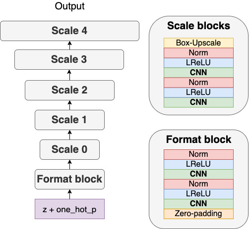
Figure 1: The architecture of the generator. The discriminator mirrors this configuration. The format block zero-pads and transforms the input noise and the one-hot attribute encoding to a $(batch\_size,128,w_{0},h_{0})$ tensor; where $w_{0}$ and $h_{0}$ are the sizes of each dimension at the first scale block input. The CNNs within each scale block have 128, 64, 64, 64, 32 feature maps, from low to high resolution, respectively. We apply pixel normalization after every convolutional layer.

Our reference architecture is a Progressive Growing GAN (P-GAN) [9], borrowed from the Computer Vision literature, which has achieved state-of-the-art results in neural audio synthesis with GANs [6]. The generator’s architecture is depicted in Figure 1. The generator $G$ samples a random vector $z$ with 128 components from a spherical Gaussian and feeds it together with the one-hot conditional information one_hot_p through a Format block and a stack of Scale blocks. The Format block turns the 1D input vector z + one_hot_p, with size 128 + 27, into a 4D convolutional input by zero-padding in the time and frequency-dimension (i.e., placing the input vector in the middle of the convolutional input with 128 + 27 convolutional maps). The Scale blocks are a stack of convolutional and box-up-sampling blocks that transform the convolutional input to the generated output signal. The discriminator $D$ is composed of convolutional and down-sampling blocks, mirroring the configuration of the generator. $D$ estimates the Wasserstein distance between the real and generated distributions [22]. We use a gradient penalty of 10.0 to enforce the Lipschitz constraint and pixel normalization at each layer. We initialize weights to zero and apply He’s constant [23] for normalizing each layer at run-time in order to ensure an equalized learning rate. Also, we use a mini-batch standard deviation before the last layer of $D$ [24]. This encourages $G$ to generate more variety and thus reduces mode collapse. For conditional model experiments, we add an auxiliary classification loss to the discriminator that learns to predict the pitch label [25].

Training is divided into phases, wherein each phase a new layer, generating a higher-resolution output, is added to the existing stack. A blending parameter $\alpha{}$ progressively fades in the gradient derived from the new layers, minimizing possible perturbation effects. We train all the models for 1.1M iterations on batches of 8 samples: 200k iterations in each of the first four phases and 300k in the last one. We employ Adam as the optimization method.

III-B Dataset

TABLE I: Audio representation configuration

Audio rep.	channels	freq. bins	time frames/instance
waveform	1	-	16000
complex	2	512	64
mag-if	2	512	64
cq-nsgt	4	97	948
cqt	2	84	256
mel	1	128	64
mfcc	1	128	64

For this work, we make use of the NSynth dataset [26], consisting of approximately 300,000 single-note audios played by more than 1,000 different instruments from 10 different families. The samples are aligned, meaning that the onset of each note is centered at time 0. It contains labels for pitch, velocity, instrument type, acoustic qualities (acoustic or electronic), and more, although, for this particular work, we only make use of the pitch information for those experiments regarding conditional models. Each sample is four seconds long, with a 16kHz sample rate. The subset of NSynth we use here only contains acoustic instruments from the brass, flutes, guitars, keyboards, and mallets families. We also trim down the audio samples from 4 to 1 seconds and only consider samples with a MIDI pitch range from 44 to 70 (103.83 - 466.16 Hz), as this is the range in which there exist the most examples from the chosen instrument types. This yields a subset of approximately 22k sounds with balanced instrument class distribution. For the evaluation, we perform an 80/20% split of the data.

All time-frequency representations, except cqt and cq-nsgt, are computed using an FFT size of 1024 and 75% overlapping. In the case of mel and mfcc, we employ a filter-bank of 128 Mel bins. For mfcc, we do not compress the Mel frequency information so as to preserve pitch information. cqt is computed using 12 bins per octave with a total of 84 bins. cq-nsgt is computed using 193 bins and assuming a complex signal. This leads to a non-symmetric spectrogram in which correlated frequency information is mirrored around the DC component. In order to make the information more local, we fold the magnitude and phase components and discard the DC. The resulting tensor sizes for each representation are summarized in Table I.

III-C Evaluation

Evaluating generative models is not straight-forward. Particularly in the case of audio synthesis, where the goal of synthesizing perceptually-realistic audio is hard to formalize. A common practice is to compare models by listening to samples and to measure their performance in classification tasks. Similarly to previous work [6], we evaluate our models against a diverse set of metrics that are common in the literature, each capturing a distinct aspect of the model’s performance.

• The Inception Score (IS) is defined as the mean KL divergence between the conditional class probabilities $p(y|x)$, and the marginal distribution $p(y)$ using the predictions of an Inception classifier [24]:

  $$\exp{\big{(}E_{x}[KL(p(y|x)||p(y))]\big{)}}$$ (1)

  Similar to [6], we adapt this metric to audio evaluation by training the Inception Net on the tasks of instrument and pitch classification from magnitude STFT spectrograms. We refer to these as Pitch Inception Score (PIS) and Instrument Inception Score (IIS), respectively. IS penalizes models whose examples are not classified into a single class with high confidence, as well as models whose examples belong to only a few of all the possible classes. We trained the pitch and instrument inception model variants on the same sub-set of the NSynth used throughout our experiments, with a train-validation split of 80% and 20%, respectively.

• Kernel Inception Distance (KID). The KID measures the dissimilarity between samples drawn independently from real and generated distributions [27]. It is defined as the squared Maximum Mean Discrepancy (MMD) between Inception representations. A lower MMD means that the generated probability distribution $P_{g}$ is closer to the real data distribution $P_{r}$. We employ the unbiased estimator of the squared MMD [28] between $m$ samples $X\thicksim P_{r}$ and $n$ samples $Y\thicksim P_{g}$, for some fixed characteristic kernel function $k$, defined as:

  $$\begin{split}\text{MMD}^{2}(X,Y)=&\quad\frac{1}{m(m-1)}\sum_{i\neq j}^{m}k(x_{i},x_{j})\\ +&\quad\frac{1}{n(n-1)}\sum_{i\neq j}^{n}k(y_{i},y_{j})\\ -&\quad\frac{2}{mn}\sum_{i=1}^{m}\sum_{j=1}^{n}k(x_{i},y_{j})\end{split}$$ (2)

  Here, we use an inverse multi-quadratic kernel (IMQ) $k(x,y)=1/(1+||x-y||^{2}/2\gamma^{2})$ with $\gamma^{2}=8$, as it has a heavier tail than a Gaussian kernel, hence, it is more sensitive to outliers. We borrow this metric from the Computer Vision literature and apply it to the audio domain.

• The Fréchet Audio Distance (FAD) compares the statistics of real and fake data computed from an embedding layer of a pre-trained VGGish model [29]. Viewing the embedding layer as a continuous multivariate Gaussian, the mean and covariance are estimated for real and fake data, and the FAD between these is calculated as:

  $$FAD=||\mu{}_{r}-\mu{}_{g}||^{2}+tr(\Sigma_{r}+\mu{}_{g}-2\sqrt{\Sigma_{r}\Sigma_{g}})$$ (3)

  where $(\mu{}_{r},\Sigma_{r})$ and $(\mu{}_{g},\Sigma{}_{g})$ are the mean and covariances of $P_{r}$ and $P_{g}$, respectively. Lower FAD means smaller distances between synthetic and real data distributions. FAD performs well in terms of robustness against noise, computational efficiency, consistency with human judgments and sensitivity to intra-class mode dropping.

IV Results

IV-A Qualitative results

We encourage the reader to listen to the audio examples provided at the accompaniment website. mag-if and complex seem to have the best-perceived quality, and are comparable to state-of-the-art works on adversarial audio synthesis (e.g., [6, 8]). We note that every representation has specific artifacts. While waveform seems to suffer from general broad-band noise, in $nsgt$ problems in reproducing plausible phase information sometimes lead to percussive artifacts (and frequency sweeps) at the beginning and end of a sample. The samples in other representations suffer from ringing (e.g., complex) or from pitch distortion (e.g., cqt).

Interpolation between random points in the latent space seems to produce particularly smooth transitions in complex, followed by mag-if, cqt, and cq-nsgt. The model trained on mel fails to faithfully reproduce the timbral characteristics of the training data, and also does not generate the required pitches in the pitch-conditional setting (it always produces the same pitch for a given $z$). As the training setup is the same for every representation, the reason for that is not clear.

IV-B Quantitative results

TABLE II: Unconditional models. Higher is better for PIS and IIS, lower is better for PKID, IKID and FAD.

Models	PIS	IIS	PKID	IKID	FAD
real data	12.5	4.0	0.000	0.000	0.01
waveform	3.7	1.8	0.083	0.291	6.46
complex	9.5	2.8	0.007	0.124	3.17
mag-if	7.3	2.7	0.015	0.149	2.71
cq-nsgt	8.1	3.4	0.012	0.041	2.11
cqt	7.8	2.6	0.013	0.112	2.55
mel	2.3	1.1	0.147	0.300	5.20
mfcc	8.9	3.0	0.008	0.080	2.92

TABLE III: Conditional models. Higher is better for PIS and IIS, lower is better for PKID, IKID and FAD.

Models	PIS	IIS	PKID	IKID	FAD
real data	12.5	4.0	0.000	0.000	0.01
waveform	3.4	2.1	0.222	0.108	1.87
complex	12.0	2.7	0.005	0.159	0.11
mag-if	12.6	3.9	0.002	0.020	0.12
cq-nsgt	7.6	3.3	0.014	0.049	0.12
cqt	12.3	3.9	0.008	0.107	2.03
mel	12.3	3.8	0.165	0.371	4.79
mfcc	9.7	3.7	0.006	0.074	2.62

TABLE IV: Metrics of post-processed real data for lossy transformations. Higher is better for PIS and IIS, lower is better for PKID, IKID and FAD.

Models	PIS	IIS	PKID	IKID	FAD
cqt	10.5	3.1	0.001	0.001	0.66
mel	12.5	3.7	0.001	0.001	0.31
mfcc	12.8	3.4	0.001	0.001	1.29

The quantitative evaluation for samples generated by the unconditional and conditional models are shown in Table II and Table III, respectively. We observe a trend that the figures get worse from complex and mag-if to mel and waveform. In some metrics, the highest quality models (complex, mag-if, and cqt) obtain results close to the real data. Furthermore, the results are generally better in the conditional setting. This is probably because the pitch-conditioning signal guides the generator in covering the variance over pitches, making it easier for the generator / discriminator pair to learn the remaining variances. Informal listening tests suggest that PKID, IKID and FAD are better aligned with perceived sound quality than PIS and IIS. In PKID, IKID and FAD (in both, the conditional and unconditional setting), the models of all representations seem to perform similarly, except mel and waveform, which both yield considerably worse results.

PIS and IIS seem to correspond better with perceived quality in the unconditional setting (with waveform and mel having low PIS and IIS) than in the conditional setting. In the latter, PIS and IIS fail to reflect the incapability of the model trained on mel to produce clear pitches, and to faithfully reproduce the timbral characteristics of the training data. Despite this, we note that both PIS and IIS are high for that model. Conversely, for data generated in the waveform domain, the PIS and IIS are low, even though pitch and instrument types can be clearly perceived in informal listening tests. This suggests that the inception models are not robust to the particular artefacts of these representations and therefore not very reliable in measuring the overall generation quality.

For lossy representations (i.e., cqt, mel and mfcc), the quantitative evaluation may suffer from a bias introduced by the lossy compression itself. Therefore, we compute the lower bounds of each representation by encoding/decoding the dataset used for our experiments in the respective transformations, and treating that as “generated data” in the evaluation. Table IV shows the results of this experiment. While cqt seems to have slightly worse lower bounds in general, the FAD of mfcc is worse than that of mel, even though there are no audible differences in the audio. Apparently the cosine-transform used to compute mfcc from mel introduces non-audible artifacts, which have considerable effect on the latent representations of the Inception model.

Table V shows the training, sampling, and inversion times associated with each model and representation. Note that training times are just rough measures, as they might be affected by variations in performance and resource availability in the training infrastructure. We can observe that, in general, representations with higher compression yield faster training and sampling times, but at the expense of slower inversion. cqt produces the best training, sampling, and inversion times trade-off, followed by the complex and mag-if representations.

TABLE V: Training, sampling and inversion times for each model

Models	training (days)	sampling (s)	inversion (s)
waveform	6.1	1.31	0.00
complex	3.5	0.20	0.01
mag-if	4.5	0.24	0.02
cq-nsgt	5.3	0.46	0.03
cqt	2.1	0.09	0.03
mel	1.5	0.04	3.69
mfcc	2.0	0.07	10.80

V Conclusion

In this work, we compared a variety of audio representations for the task of adversarial audio synthesis of pitched sounds. We performed quantitative and qualitative evaluation, and reported on training, generation, and inversion times. We found that complex and mag-if yield the best quantitative metrics, which is also aligned with informal listening of the generated samples. This is interesting, as we are not aware that complex was used before in audio generation. We also found that evaluation metrics are generally aligned with perceived quality, but in some cases they can be sensitive to non-audible representation-specific artifacts (e.g., FAD), or yield figures which seem over-optimistic when listening to the examples (e.g., PIS and IIS).

References

- [1] S. Dieleman and B. Schrauwen, “End-to-end learning for music audio,” in ICASSP, Florence, Italy, May 2014, pp. 6964–6968.
- [2] Z. Zhu, J. H. Engel, and A. Y. Hannun, “Learning multiscale features directly from waveforms,” in INTERSPEECH, San Francisco, CA, USA, Sept. 2016, pp. 1305–1309.
- [3] A. van den Oord, S. Dieleman, H. Zen, K. Simonyan, O. Vinyals, A. Graves, N. Kalchbrenner, A. W. Senior, and K. Kavukcuoglu, “Wavenet: A generative model for raw audio,” CoRR, vol. abs/1609.03499, 2016.
- [4] S. Vasquez and M. Lewis, “Melnet: A generative model for audio in the frequency domain,” CoRR, vol. abs/1906.01083, 2019.
- [5] I. J. Goodfellow, J. Pouget-Abadie, M. Mirza, B. Xu, D. Warde-Farley, S. Ozair, A. C. Courville, and Y. Bengio, “Generative adversarial nets,” in NeurIPS, Montreal, Quebec, Canada, Dec. 2014, pp. 2672–2680.
- [6] J. Engel, K. K. Agrawal, S. Chen, I. Gulrajani, C. Donahue, and A. Roberts, “GANsynth: Adversarial neural audio synthesis,” in ICLR, New Orleans, LA, USA, May 2019.
- [7] A. Marafioti, N. Holighaus, N. Perraudin, and P. Majdak, “Adversarial generation of time-frequency features with application in audio synthesis,” CoRR, vol. abs/1902.04072, 2019.
- [8] C. Donahue, J. McAuley, and M. Puckette, “Adversarial audio synthesis,” in ICLR, New Orleans, LA, USA, May 2019.
- [9] T. Karras, T. Aila, S. Laine, and J. Lehtinen, “Progressive growing of GANs for improved quality, stability, and variation,” CoRR, vol. abs/1710.10196, 2017.
- [10] B. McFee, C. Raffel, D. Liang, D. P. Ellis, M. McVicar, E. Battenberg et al., “librosa/librosa: 0.7.2,” Jan. 2020.
- [11] S. Dieleman, A. van den Oord, and K. Simonyan, “The challenge of realistic music generation: modelling raw audio at scale,” in NeurIPS, Montréal, Canada, Dec. 2018, pp. 8000–8010.
- [12] B. Boashash, “Estimating and interpreting the instantaneous frequency of a signal. ii. algorithms and applications,” Proc. of the IEEE, vol. 80, no. 4, pp. 550–568, Apr. 1992.
- [13] J. C. Brown, “Calculation of a constant-Q spectral transform,” J. Acoust. Soc. Am., vol. 89, no. 1, pp. 425–434, 1991.
- [14] T. Lidy, “CQT-based convolutional neural networks for audio scene classification and domestic audio tagging,” in DCASE, Sept. 2016.
- [15] P. Esling, A. Chemla-Romeu-Santos, and A. Bitton, “Generative timbre spaces with variational audio synthesis,” CoRR, vol. abs/1805.08501, 2018.
- [16] C. Schörkhuber and A. Klapuri, “Constant-Q transform toolbox for music processing,” in SMC, Barcelona, Spain, July 2010, pp. 3–64.
- [17] G. A. Velasco, N. Holighaus, M. Doerfler, and T. Grill, “Constructing an invertible constant-Q transform with nonstationary gabor frames,” DAFx, Sept. 2011.
- [18] S. S. Stevens, J. Volkmann, and E. B. Newman, “A scale for the measurement of the psychological magnitude pitch,” J. Acoust. Soc. Am., vol. 8, no. 3, pp. 185–190, 1937.
- [19] D. W. Griffin and J. S. Lim, “Signal estimation from modified short-time fourier transform,” in ICASSP, Boston, Massachusetts, USA, Apr. 1983, pp. 804–807.
- [20] S. B. Davis and P. Mermelstein, “Comparison of parametric representations for monosyllabic word recognition in continuously spoken sentences,” IEEE Trans. Acoust. Speech, Signal Process., pp. 357–366, 1980.
- [21] E. Ravelli, G. Richard, and L. Daudet, “Audio signal representations for indexing in the transform domain,” IEEE Trans. Audio, Speech, Language Process., vol. 18, no. 3, pp. 434–446, 2010.
- [22] I. Gulrajani, F. Ahmed, M. Arjovsky, V. Dumoulin, and A. C. Courville, “Improved training of Wasserstein GANs,” in NeurIPS, Long Beach, CA, USA, Dec. 2017, pp. 5769–5779.
- [23] K. He, X. Zhang, S. Ren, and J. Sun, “Delving deep into rectifiers: Surpassing human-level performance on imagenet classification,” in ICCV, Santiago, Chile, Dec. 2015, pp. 1026–1034.
- [24] T. Salimans, I. J. Goodfellow, W. Zaremba, V. Cheung, A. Radford, and X. Chen, “Improved techniques for training GANs,” in NeurIPS, Barcelona, Spain, Dec. 2016, pp. 2226–2234.
- [25] A. Odena, C. Olah, and J. Shlens, “Conditional image synthesis with auxiliary classifier GANs,” in ICML, Sydney, NSW, Australia, Aug. 2017, pp. 2642–2651.
- [26] J. Engel, C. Resnick, A. Roberts, S. Dieleman, M. Norouzi, D. Eck, and K. Simonyan, “Neural audio synthesis of musical notes with wavenet autoencoders,” in ICML, Sydney, NSW, Australia, Aug. 2017, pp. 1068–1077.
- [27] M. Binkowski, D. J. Sutherland, M. Arbel, and A. Gretton, “Demystifying MMD GANs,” in ICLR, Vancouver, BC, Canada, Apr. 2018.
- [28] A. Gretton, K. M. Borgwardt, M. J. Rasch, B. Schölkopf, and A. J. Smola, “A kernel two-sample test,” J. of Mach. Learn. Res., vol. 13, pp. 723–773, 2012.
- [29] K. Kilgour, M. Zuluaga, D. Roblek, and M. Sharifi, “Fréchet Audio Distance: A metric for evaluating music enhancement algorithms,” CoRR, vol. abs/1812.08466, 2018.