Structured and Localized Image Restoration

Abstract

We present a novel approach to image restoration that leverages ideas from localized structured prediction and non-linear multi-task learning. We optimize a penalized energy function regularized by a sum of terms measuring the distance between patches to be restored and clean patches from an external database gathered beforehand. The resulting estimator comes with strong statistical guarantees leveraging local dependency properties of overlapping patches. We derive the corresponding algorithms for energies based on the mean-squared and Euclidean norm errors. Finally, we demonstrate the practical effectiveness of our model on different image restoration problems using standard benchmarks.

1 Introduction

After decades of work, image processing is still a vibrant research field, particularly well suited to modern machine learning technology, given that it is often easy to generate clean/corrupted image pairs, and more pertinent than ever with the ubiquitous use of smartphone cameras, and many applications in personal photography [1], microscopy [47] and astronomy [40], for example. Given a clean image $x$, a known (in general) linear operator $B$ such as downsampling or blur, and additive noise $\varepsilon$ with standard deviation $\sigma$, the degraded image $y$ is typically modelled as

$$y=Bx+\varepsilon.$$ (1)

The operator $B$ is problem specific, e.g., for denoising it is the identity, and for deblurring it is a sparse matrix standing for a convolution with some blur kernel[25]. Solvers for this problem date back from Wiener’s seminal work [48], that cast image restoration as the minimization of some mean-squared error (MSE). Decades later, Rudin et al. [35] proposed a variational formulation of image denoising using both a data term and a total variation prior. A discretized version of this approach and its optimization were proposed by Wang et al. [46] and it has since been extended to various tasks such as non-blind deblurring using much powerful priors [23, 52].

In this work, we propose a non-parametric general image restoration algorithm based on localized structured prediction [9, 11] and non-linear multi-task learning [12]. In particular, we adapt to patch-based image restoration the theoretical framework of [9] for energy minimization under local task-specific constraints. Our approach is reminiscent of that of Zoran and Weiss [52] and its patch-based energy function, but it also combines ideas from example-based [17, 20], variational [23, 52] and data-driven methods [42, 8] into a single model. A crucial and distinctive feature of our approach is that we have a complete statistical analysis of the corresponding prediction error. In particular, we provide an interpretable error upper bound explicitly parameterized by quantities depending on local dependency properties of the natural images. Most image restoration works do not provide a theoretical analysis, with notable exceptions such as [26] in the context of online dictionary learning. Our estimator is based on a convex energy function that can be minimized exactly, contrary to standard example-based methods that often rely on approximation of Markov random fields [17] or local and non-local averaging techniques [5, 13]. Data-driven methods such as sparse coding [15, 49] often assume an unrealistic i.i.d. patch model, whereas our framework explicitly accounts for the patch correlations. Although CNN-based methods achieve state-of-the-art results in many restoration tasks [51, 14, 50], they often ignore the underlying image degradation model, require a very large number of training data and suffer from a lack of interpretability and theoretical guarantees. Instead, the proposed approach only requires a limited number of examples since it leverages the interplay of the the forward model with the local properties of the data at the patch level, and it is fully interpretable. Finally, our approach is highly modular, and many of its components can be changed and/or learnt while ensuring convergence, similar to Ciliberto et al. [9, 11] in the context of statistical learning theory. Changing these components shapes the form of the energy and can lead to specific solvers for each situation. Concretely, our contributions include:

• A new image restoration framework based on localized structured prediction [9] and non-linear multi-task learning [12] that bridges statistical learning theory and image restoration. The estimator is written as a minimizer of an energy with a learnable prior defined on patches.

• A theoretical analysis of the estimator with explicit quantities depending on the local dependency properties of the problem.

• Two efficient implementations: For the MSE-based solver, we solve a linear system with conjugate gradient. For the Euclidean norm-based solver, we introduce a splitting scheme that alternates between conjugate gradient and dual coordinate ascent.

• An experimental validation of the methods on standard benchmarks for non-blind deblurring and upsamling. We achieve results comparable or better than standard variational methods. Our goal is not to beat the state of the art but to showcase the practical abilities of this general framework to solve image restoration problems.

Related work. Image restoration methods can be divided into three groups.

Example-based methods restore patches based on similar ones taken from an external dataset [17, 41] or the image at hand by exploiting self similarities in a given neighborhood [13, 5, 22] or at different scales [19]. For example, [17] addresses image upsampling by comparing low-resolution patches in the target image with those in an external dataset retrieving the nearest neighbors, and copying and pasting their high-resolution version into the restored image. In [13], the authors group and average similar patches in the image to remove noise.

Energy-based methods minimize an objective function typically composed of a fitting term enforcing Eq. 1 and a penalty term favoring solutions exhibiting features of natural images. For instance, the total variation prior [35, 46, 23] favors images with sharp edges, while the prior on patches of [52] uses the centroids of a Gaussian mixture model (GMM) to guide the restoration. A drawback of these methods is that they rely on handcrafted priors which might not capture all aspects of natural images.

Learning-based methods minimize an empirical risk based on a dataset of pairs of clean and degraded images. In particular, dictionary learning methods estimate a small number of atoms to encode sparse models of patches and can be used in tasks such as denoising [15, 27, 25] and upsampling [49]. Most learning-based models are parametric (see [42, 7] for counter examples) and learnt in a supervised manner, often as convolutional neural networks (CNNs), especially in problems like denoising [51], upsampling [14] or deblurring [51]. Recently, data-driven and energy-based methods have also been combined to learn the minimizer of energies with tunable parameters in the regularizer [50, 8].

Figure 1: Given a degraded (blurry here) image $y$, the estimator $\widehat{\bf x}$ predicts a sharp image $\widehat{\bf x}(y)$. The vector of weights $\alpha$ is computed by comparing the patches $y_{p}$ from the image to the patches $\text{y}^{(i)}$ from an external set, associated with clean versions $\text{x}^{(i)}$. These weights are used to construct an energy function that favors sharp patches $x_{p}$ similar to samples $\text{x}^{(i)}$. Finally, the estimated sharp image is a minimizer of this energy, penalized with the formation model of Eq. 1.

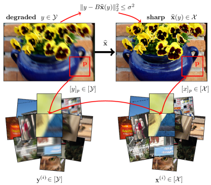
2 Proposed framework

Let $\mathcal{X}$ be the space of natural images and $\mathcal{Y}$ the space of degraded ones. The goal of image restoration is to estimate a function ${\bf x}:\mathcal{Y}\rightarrow\mathcal{X}$ that computes the sharp image ${\bf x}(y)$ from a degraded image $y$. Concretely, the degradation process is modeled in terms of a probability distribution $\rho$ on $\mathcal{X}\times\mathcal{Y}$, and the goal is to find the function ${\bf x}^{\star}:\mathcal{Y}\xrightarrow{}\mathcal{X}$ that minimizes the expected risk

$$\mathcal{E}({\bf x})=\operatorname{\mathbb{E}}_{(y,x)\sim\rho}~{}L({\bf x}(y),x),$$ (2)

using only the observed dataset $(y^{(i)},x^{(i)})_{i=1}^{n}$ sampled from $\rho$, where $L$ is a loss between images. The formulation above is very general and standard to supervised learning problems [44]. Here, instead, we want to specialize the learning process to leverage the properties of the image formation model. By enforcing (1), we can restrict the class of estimators to functions ${\bf x}:\mathcal{Y}\to\mathcal{X}$ satisfying $\|y-B{\bf x}(y)\|_{2}^{2}\leq\sigma^{2}$ for all $y\in\mathcal{Y}$. This is equivalent [12] to

$${\bf x}^{\star}_{\sigma}(y)=\operatorname*{arg\;min}_{\|y-Bx\|^{2}\leq\sigma^{2}}~{}\Omega_{L}^{\pi}(x~{}|~{}y),\hskip 8.5359pt\text{where}\hskip 8.5359pt\Omega_{L}^{\pi}(x~{}|~{}y)=\mathbb{E}_{x^{\prime}\sim\pi_{y}}L(x,x^{\prime}),$$ (3)

where $\pi_{y}(x)=\rho(x~{}|~{}y)$ is the conditional distribution of $x$ given $y$. Note that the conditional distribution $\pi$ is unknown, and so the quantity $\Omega_{L}^{\pi}(x~{}|~{}y)$ cannot in general be computed exactly. By Lagrangian duality, we can rewrite for a suitable $\gamma\geq 0$ the optimization problem as

$$\operatorname*{arg\;min}_{x\in\mathcal{X}}~{}\Omega_{L}^{\pi}(x~{}|~{}y)+\frac{\gamma}{2}\|y-Bx\|_{2}^{2}.$$ (4)

2.1 Leveraging local priors: localized structured prediction

We can further specialize the class of estimators considered by leveraging the strong structural properties at a local level that are common in natural images [25]. Let us consider decompositions of the images $x$ and $y$ into overlapping patches indexed by $p\in P$, where $P$ is the set of patch identifiers. Denote by $x_{p}$ and $y_{p}$ the $p$-th patch of the sharp image and degraded image, and denote by $[\mathcal{X}],[\mathcal{Y}]$ the corresponding spaces of patches. In vector form, $x_{p}$ and $y_{p}$ correspond to a subset of coordinates of $x,y$. We assume that the image degradation problem is local, i.e., $y_{p}$ is determined by $x_{p}$ and $B$. Thus, estimating $x$ from $y$ can be seen as a multi-task learning problem, where the function $y\mapsto x$ is factored in a group of functions $y_{p}\mapsto x_{p}$ collaboratively solving the global problem. We similarly assume that the degradation function is stationary with respect to the position of the patch in the image, that is, the functions $y_{p}\mapsto x_{p}$ are independent of the patch identifier $p$. As in [9] we formalize the behavior described above as follows.

Between-locality assumption: $x_{p}$ is conditionally independent from $y$ given $y_{p}$. Moreover the following holds for all patches $p,p^{\prime}\in P$,

$$\pi_{y_{p}}(x_{p})=\pi_{y_{p^{\prime}}}(x_{p^{\prime}}).$$ (5)

Note that assumption (5) uses the stationarity mentioned above, as the conditional distribution of patches $\pi_{y_{p}}(x_{p})$ between $x_{p}$ and $y_{p}$ is independent of the index $p$. It is then natural to consider losses $L$ in (4) that measure the global error between two images in terms of errors on the single patches

$$\textstyle{L(x,x^{\prime})=\frac{1}{|P|}\sum_{p\in P}\ell(x_{p},x^{\prime}_{p})},$$ (6)

where $\ell$ is a loss function between patches. For instance, one can take $\ell$ to be the mean-squared error $\|x_{p}-x_{p}^{\prime}\|_{2}^{2}$, which decomposes additively over the pixels of the pair of patches, making the predictions independent for every pixel of the image. If one considers instead the non-squared Euclidean norm $\|x_{p}-x_{p}^{\prime}\|_{2}$, then the problem is solved by taking into account inter-dependencies between overlapping patches [21]. Given assumption (5), it is convenient to drop the patch index and designate patches without specifying that they come from a certain location of an image. In the rest of the paper we will denote by x and y two generic patches belonging to $[\mathcal{X}]$ and $[\mathcal{Y}]$, respectively. Note that with this construction, the regularizer decomposes additively as

$$\textstyle\Omega_{L}^{\pi}(x~{}|~{}y)=\frac{1}{|P|}\sum_{p\in P}\Omega_{\ell}^{\pi}(x_{p}~{}|~{}y_{p}),\quad\textrm{where},\quad\Omega_{\ell}^{\pi}(\text{x}~{}|~{}\text{y})=\operatorname{\mathbb{E}}_{\text{x}^{\prime}\sim\pi_{\text{y}}}\ell(\text{x},\text{x}^{\prime}),$$ (7)

for all $\text{x}\in[\mathcal{X}],\text{y}\in[\mathcal{Y}]$. Then, our problem takes the form

$$\textstyle\operatorname*{arg\;min}_{x\in\mathcal{X}}~{}\frac{1}{|P|}\sum_{p\in P}\Omega_{\ell}^{\pi}(x_{p}~{}|~{}y_{p})+\frac{\gamma}{2}\|y-Bx\|_{2}^{2},$$ (8)

enforcing at the same time prior knowledge of the problem at the global level via the variational representation of the formation model (1) and at the local level via the data-driven regularizer on patches. However, as we do not have access to the conditional distribution $\pi_{\text{y}}(\text{x})$, this term cannot be computed exactly. We now show how to approximate it from supervisory data.

2.2 Construction of the estimator

The goal is to learn the function $\text{y}\mapsto\Omega_{\ell}^{\pi}(\text{x}~{}|~{}\text{y})$ for every $\text{x}\in[\mathcal{X}]$ from a dataset of $m$ pairs of patches $(\text{y}^{(i)},\text{x}^{(i)})$ extracted from images degraded by $B$ and the associated clean images. We want to construct the estimator simultaneously for every sharp patch x. In order to do this, following [11, 9], we consider estimators that are linear combinations of the loss function evaluated at the data points

$$\textstyle{\Omega_{\ell}^{\pi}(\text{x}~{}|~{}\text{y})\approx\sum_{i=1}^{m}\alpha_{i}(\text{y})\ell(\text{x},\text{x}^{(i)})},$$ (9)

where $\alpha_{i}(\text{y})$ are scalar coefficients learnt from the dataset of patches. For any degraded patch y, $\alpha_{i}(\text{y})$ can be interpreted as a measure of similarity between y and the patch $\text{y}^{(i)}$ of the training dataset. Finally, we define the estimator $\widehat{\bf x}(y)$ as:

$$\widehat{\bf x}(y)\in\operatorname*{arg\;min}_{x\in\mathcal{X}}~{}\frac{1}{|P|}\sum_{p\in P}\sum_{i=1}^{m}\alpha_{i}(y_{p})\ell(x_{p},\text{x}^{(i)})+\frac{\gamma}{2}\|y-Bx\|_{2}^{2}.$$ (10)

We provide two ways of computing the coefficients $\alpha_{i}$.

Kernel ridge regression (KRR). To derive the estimator we start from the observation that when we fix $\text{x}\in[\mathcal{X}]$, then $\textstyle{\Omega_{\ell}^{\pi}(\text{x}~{}|~{}\text{y})}$ is just a function from $[\mathcal{Y}]$ to $\mathbb{R}$, that we denote $g_{\text{x}}^{\star}:[\mathcal{Y}]\rightarrow\mathbb{R}$ for convenience. The idea now is to learn $g_{\text{x}}^{\star}$ from data. In particular, note that $g^{*}_{\text{x}}$ is the minimizer over $\{g:[\mathcal{Y}]\rightarrow\mathbb{R}\}$ of the least-squares expected risk $\operatorname{\mathbb{E}}_{(\text{x}^{\prime},\text{y}^{\prime})\sim\rho}(g(\text{y}^{\prime})-\ell(\text{x},\text{x}^{\prime}))^{2}$. Then, $g_{\text{x}}^{\star}$ can be estimated from a dataset $(\text{y}^{(i)},\ell(\text{x},\text{x}^{(i)}))$ of $m$ pairs using regularized empirical risk minimization and standard techniques from supervised machine learning as kernel ridge regression [36]. More specifically, let $\mathcal{G}$ be a reproducing kernel Hilbert space (RKHS) with associated positive kernel $k:[\mathcal{Y}]\times[\mathcal{Y}]\rightarrow\mathbb{R}$ over pairs of patches of degraded images [3]. Then, for every $\text{x}\in[\mathcal{X}]$, the function $g_{\text{x}}^{\star}$ can be approximated by $\widehat{g}_{\text{x}}$ as

$$\widehat{g}_{\text{x}}~{}=~{}\textstyle{\operatorname*{arg\;min}_{g\in\mathcal{G}}\frac{1}{m}\sum_{i=1}^{m}(g(\text{y}^{(i)})-\ell(\text{x},\text{x}^{(i)}))^{2}+\frac{\lambda}{2}\|g\|_{\mathcal{G}}^{2}},$$ (11)

where $\|g\|_{\mathcal{G}}$ denotes the norm of $g$ in ${\cal G}$ and $\lambda$ is a regularization parameter. The solution takes the form of (9) where the vector $\alpha(\text{y})$ is the solution of the linear system

$$(K+m\lambda I)\alpha(\text{y})=v(\text{y})\in\mathbb{R}^{m}.$$ (12)

Here, $v(\text{y})_{i}=k(\text{y},\text{y}^{(i)})$ and $K$ is a matrix in $\mathbb{R}^{m\times m}$ defined by $K_{ij}~{}=~{}k(\text{y}^{(i)},\text{y}^{(j)})$,

Nadaraya-Watson (NW). Conversely, $\text{y}\mapsto\Omega^{\pi}_{\ell}(\text{x},\text{y})$ can also be estimated with the Nadaraya-Watson estimator [30], a version of kernel density estimation [33] for regression. We have

$$\alpha(\text{y})=\frac{1}{\mathbbm{1}^{\top}v(\text{y})}v(\text{y})\in\mathbb{R}^{m},$$ (13)

where $\mathbbm{1}$ is a vector of size $n$ with all entries equal to 1. Contrary to (12), all coefficients are positive and their computation does not involve the kernel matrix $K$. In the following Section 3, we analyze the statistical properties of the estimator (10) when the $\alpha$’s are computed using KRR.

3 Statistical Guarantees

The goal of this section is twofold. First we show that the estimate $\widehat{\bf x}$ in Eq. 10 approaches the optimal estimator ${\bf x}^{\star}$ minimizing (2) when the size of the patch dataset tends to infinity. Moreover, we explicitly characterize the convergence rate at which this happens. For simplicity, and based on the analysis of [9], we assume that the coefficients $\alpha$ are computed using kernel ridge regression (12).

Let us first define the sampling scheme to generate patches from images. We generate a dataset of clean and degraded pairs of patches $(\text{y}^{(i)},\text{x}^{(i)})$ ($i=1,\dots,m$) by sub-sampling uniformly patches from $n$ pairs of clean and degraded-by-$B$ images. We theoretically justify and validate experimentally why subsampling patches, which corresponds to $m\ll|P|n$, is a good choice.

In order to simplify the analysis, we work with the constrained version of the minimizer $\widehat{\bf x}(y)$ defined in Eq. 10, where the estimated regularizers (9) are minimized over the constraint $\|y-Bx\|_{2}^{2}\leq\sigma^{2}$, instead of the penalized version. Our main result is a bound on the excess risk $\mathcal{E}(\widehat{\bf x})-\mathcal{E}({\bf x}_{\sigma}^{\star})$ depending on the number of images $n$, the number of subsampled patches $m$, and interpretable constants describing local dependency properties of the problem. More specifically, the bound on the excess risk depends on the quantities $c_{B,\sigma}$ and $q$ defined as:

$$c_{B,\sigma}=\frac{\operatorname{\mathbb{E}}_{y\sim\rho_{\mathcal{Y}}}\operatorname{diam}(\mathcal{C}_{B,\sigma}(y))}{\operatorname{diam}(\mathcal{X})}\leq 1,\quad q=\frac{1}{|P|r^{2}}\sum_{p,p^{\prime}\in P}\operatorname{\mathbb{E}}_{y,y^{\prime}}C_{p,p^{\prime}}(y,y^{\prime}),$$ (14)

where $\operatorname{diam}$ stands for diameter; $\mathcal{C}_{B,\sigma}(y)=\{x\in\mathcal{X}~{}|~{}\|Bx-y\|_{2}\leq\sigma\}\subseteq\mathcal{X}$ is the constraint set defined by the formation model (1); $C_{p,p^{\prime}}(y,y^{\prime})=k(y_{p},y_{p^{\prime}})^{2}-k(y_{p},y^{\prime}_{p^{\prime}})^{2}$ is a measure of similarity between $y$ and $y^{\prime}$; and $r^{2}=\sup_{\text{y}\in[\mathcal{Y}]}k(\text{y},\text{y})$ is the maximum squared norm of the features. We recall that $k$ is the kernel computed from the degraded patches used to train KRR (Section 2.2). The constant $c_{B,\sigma}$ is a ratio between the expected diameter of the constraint set and the diameter of the full space of sharp images. The smaller the ratio, the more informative is the knowledge of the formation model (1) for the learning task. The constant $q$ measures the total correlation between patches of image $y$. It satisfies $q\approx|P|$ if there is large correlation between patches and $q\approx 0$ if they are mostly independent. This is essentially the same quantity appearing in the analysis by [9], which in that case is the total correlation of the parts of a generic structured object (see Example 1 of [9]). To state the theorem we need a smoothness assumption on the loss and on the target distribution. Let the set of patches be defined respectively as $[\mathcal{X}]=[-1,1]^{d_{\mathcal{X}}\times d_{\mathcal{X}}}$ and $[\mathcal{Y}]=\mathbb{R}^{d_{\mathcal{Y}}\times d_{\mathcal{Y}}}$, with $d_{\mathcal{X}},d_{\mathcal{Y}}\in\mathbb{N}$. Denote by $W^{s}_{2}(Z)$ the Sobolev space of smoothness $s>0$ in a set $Z$, i.e., the space of functions with square-integrable weak derivatives up to order $s$ [2].

Assumption on the loss $\boldsymbol{\ell}$. Let $\ell_{\text{x}}$ be defined as $\text{x}^{\prime}\mapsto\ell(\text{x}^{\prime},\text{x})$. There exists $C$ in $(0,\infty)$ and $s\geq(d_{\mathcal{X}}^{2}+1)/2$ such that $\sup_{\text{x}\in[\mathcal{X}]}\|\ell_{\text{x}}\|_{W^{s}_{2}([\mathcal{X}])}\leq C$.

Assumption on the target distribution. Let $m\in\mathbb{N}$ s.t. $W^{m}_{2}([\mathcal{Y}])\subseteq{\mathcal{H}}$ where $\mathcal{H}$ is the reproducing kernel Hilbert space associated to the kernel $k$ [3, 4]. For example, $m=d_{\mathcal{Y}}^{2}/2+1$ for the Laplacian kernel $k(\text{y},\text{y}^{\prime})=e^{-\|\text{y}-\text{y}^{\prime}\|}$. We require $\rho(x|y)$ to be a density and satisfy $\rho(x|y)\in W^{m}_{2}([\mathcal{X}]\times[\mathcal{Y}]).$

Theorem 3.1 (Generalization bound).

Assume that between-locality (5) holds and that $\rho$ and $\ell$ satisfy the assumptions above. If the regularization parameter of KRR (12) is set to $\lambda=r(\frac{1}{m}+\frac{q}{|P|n})^{1/2}$, then the following holds:

$$\left|\operatorname{\mathbb{E}}\mathcal{E}(\widehat{\bf x})-\mathcal{E}({\bf x}^{\star}_{\sigma})\right|\leq Cc_{B,\sigma}^{1/2}\left(\frac{1}{m}+\frac{1+q}{|P|n}\right)^{1/4},$$ (15)

where $C\geq 0$ is a constant independent of the $n,m,P,B$ and $\sigma$.

The main difference with the analysis of [9] is the constant $c_{B,\sigma}$. In Appendix A the theorem is proved under more general assumptions on $\rho,\ell$ relating their regularity to the reproducing kernel Hilbert space associated to $k$. The proof is based on the analysis by [12] and [9]. The assumption on $\ell$ that we make here for the sake of readability is quite mild and it is satisfied by many loss functions including squared loss and Euclidean loss (see Section A.4). The condition on the data distribution for Theorem 3.1 to hold are common for this kind of analysis [6] and in structured prediction settings [10, 9, 11]. See in Appendix A a more general statement with respect to the kernel $k$.

Effect of patch correlation. Theorem 3.1 states that the statistical performance of the estimator depends on $q$, i.e., the amount of correlation between patches. In particular, large correlation translates into $q\approx|P|$, leading to a rate of $O(n^{-1/4})$, while small correlation improves the rate up to $O(m^{-1/4})$ (remember that $m\gg n$ in general) and up to $O((n|P|)^{-1/4})$ when taking $m\propto n|P|$. This is particularly beneficial in problems with a large number of patches and allows to achieve low prediction error even with $n$ small, i.e., few training examples. The intuition is the following: when the patches from which we learn are independent, the estimators at the patch level have better performance than when they are highly correlated, as more information is present at learning time. This creates a trade-off between the size of the patches and statistical performance: for large patches the between-locality property is more likely to hold, but dependency is stronger due to overlapping. In our experiments, we take $n=4$, $|P|\approx 10^{5}$ (e.g. a 256 $\times$ 256 image contains $|P|=62001$ $8\times 8$ overlapping patches) and we show that $q\ll|P|$ in Section C.1. This justifies why selecting $m=10^{4}$ patches is enough to obtain good performance.

Effect of the fitting term. The ratio $c_{B,\sigma}\leq 1$ measures the statistical complexity of learning with the loss (2) under the constraint $\|y-Bx\|_{2}^{2}\leq\sigma^{2}$. Indeed, if the diameter of the constraint set is small, then the estimator will require less samples to achieve small error. If the constraint is removed, the constant becomes $\lim_{\sigma\to\infty}c_{B,\sigma}=1$. Moreover, it can be explicitly bounded for multiple settings. For denoising it is $\min(\sigma/\operatorname{diam}(\mathcal{X}),1)$, and so the magnitude of the noise appears as a multiplying factor in the bound (15). For upsampling with a factor $k$ and noise $\sigma=0$ it is $k^{-1/2}$, and for inpainting with a proportion of $s$ missing pixels from the image and $\sigma=0$ is $s^{1/2}$ (Section A.2).

4 Algorithm

  $z_{p}^{1}=x_{p}+1/\beta\sum_{i=1}^{m}\mu_{i}^{(0)}$ ;

  for $k=1,\dots,K$ do

     Pick $i$ at random in $\{1,...,m\}$ or perform gap sampling ;

     $b_{i}^{k}=z_{p}^{k}-\mu_{i}^{k}/\beta-\text{x}^{(i)}$ ;

     $\mu_{i}^{k+1}=-b_{i}^{k}\min(\alpha_{i}(y_{p})/\|b_{i}^{k}\|_{2},\beta)$ ;

     $z_{p}^{k+1}=z_{p}^{k}+(\mu_{i}^{k+1}-\mu_{i}^{k})/\beta$ ;

  end for

Algorithm 1 SDCA for solving (18) with Euclidean loss and NW estimator.

We now present the algorithmic scheme to compute our estimator for any loss $\ell$ and detail the specific cases of the MSE and Euclidean loss. For the sake of presentation, we remove the factor $|P|^{-1}$ in (10) and re-define the parameter $\gamma$ as $\gamma|P|$.

Least squares. When $\ell$ is the mean-squared error, the solution of (10) can be obtained by solving

$$\textstyle{\Big{(}\gamma B^{\top}B+\sum_{p\in P}\sum_{i=1}^{m}\alpha_{i}(y_{p})R_{p}^{\top}R_{p}\Big{)}x=\gamma B^{\top}y+\sum_{p\in P}\sum_{i=1}^{m}\alpha_{i}(y_{p})R_{p}^{\top}\text{x}^{(i)}},$$ (16)

where $R_{p}$ is a matrix that extracts the $p$-th patch $x_{p}$ from an image $x$ and $R_{p}^{\top}$ replaces $x_{p}$ at its initial location in $x$. This can be done using conjugate gradient descent. The problem is easy to solve because it is decomposable pixel-wise since the mean-squared error is separable, as already noted in Section 2.1. This is computationally very efficient, but in general not entirely satisfactory from a modeling viewpoint, since each patch of the sharp image represents an element composed of pixels that are shared with other patches, and thus each pixel is strongly dependent on its neighborhood.

Generic loss. For a generic loss $\ell$, we use the half-quadratic splitting (HQS) algorithm [18], decomposing the energy into simpler sub-problems. We introduce $|P|$ variables $z_{p}$ and solve

$$\min_{x,z_{1},\dots,z_{P}}~{}\sum_{i=1}^{m}\sum_{p\in P}\alpha_{i}(y_{p})\ell(z_{p},\text{x}^{(i)})+\frac{\gamma}{2}\|y-Bx\|_{2}^{2}+\frac{\beta}{2}\|x_{p}-z_{p}\|_{2}^{2}.$$ (17)

HQS outperforms in our experiments the alternating direction method of multipliers (ADMM) [32]. By choosing $x_{p}^{(0)}$ as $y_{p}$ for all $p$, the HQS algorithm performs at each iteration $t$

$$z_{p}^{(t+1)} = \textstyle{\operatorname*{arg\;min}_{z_{p}}\sum_{i=1}^{n}\alpha_{i}(y_{p})\ell(z_{p}^{(t)},\text{x}^{(i)})+\beta^{(t)}/2\|z_{p}^{(t)}-x_{p}^{(t)}\|_{2}^{2},\quad\forall p\in P,}$$ (18)

$$x^{(t+1)} = \textstyle{\operatorname*{arg\;min}_{x}\sum_{p\in P}\beta^{(t)}\|z_{p}^{(t+1)}-x_{p}^{(t)}\|_{2}^{2}+\gamma/2\|y-Bx^{(t)}\|_{2}^{2},}$$ (19)

$$\beta^{(t+1)} = \delta\beta^{(t)},$$ (20)

where $\beta^{(0)}$ a positive scalar and $\delta>1$ such that $\beta^{(t)}=\delta^{t}\ \beta^{(0)}$ exponentially grows to $+\infty$. The $x$ update (19) is a least-squares problem analogous to (16), and the $z_{p}$ updates (18) have the form of a weighted-by-$\alpha$ quadratically regularized empirical risk minimization problem. As shown in Section B.1, convexity of the objective is guaranteed if the coefficients are computed using KRR and $\ell$ is convex in its first argument, so the problem remains tractable. The update can be solved using algorithms for finite-sums such as full-gradient methods [28] or stochastic methods where the individual losses are not required to be all convex [37] (see Section B.2). We now present an efficient algorithm when $\ell$ is the Euclidean loss and the $\alpha$’s are computed using the NW estimator (13).

Euclidean loss with Nadaraya-Watson estimator. The individual losses in the finite sum of (18) are all convex when using the NW estimator, as the $\alpha$’s are all positive. In this case, we can use the stochastic dual coordinate ascent (SDCA) algorithm of [39]. It is a stochastic dual algorithm such that at each iteration it selects an index $i\in[n]$ at random, and maximizes the dual objective w.r.t. to the dual variable $\mu_{i}$. For the Euclidean loss, this maximization has a closed form solution as it is a projection into an $\ell_{2}$ ball. The method has linear convergence, is hyperparameter free, and the dual gap can be used as a termination criterion, yielding a fast and efficient solver for problem (18). Moreover, we perform non-uniform sampling by selecting the index $i\in[n]$ according to the magnitude of the individual dual gaps (see Section B.3.2). The algorithm is detailed in Algorithm 1 and our code for SDCA with gap sampling is given in Section B.3.

5 Experiments

We experimentally validate the proposed algorithms for upsampling and deblurring, showing results on par with standard variational methods. Our code will be made available and further experimental results can be found in Appendix C and Appendix D.

Implementation details. We consider the overlapping patches of the image as its set of parts $P$, as done in [41, 52]. We randomly select $m=10,000$, $8\times 8$-patches from $n=4$ training images of the BSD300 dataset [29] to build the external dataset. Increasing $m$ further improves the results and this value is thus a good compromise between speed and accuracy. To compute $\alpha$, we use a Gaussian kernel comparing the discrete cosine transform (DCT) coefficients of the patches, as in [13]. When predicting $z_{p}$ with SDCA, the training patches $\text{x}^{(i)}$ and the current value of $x_{p}$ are centered for better reconstruction [27, 25, 52, 41]. The mean of $x_{p}$ is added to $z_{p}$ at the end of the SDCA loop. We recompute $\alpha$ at each iteration $t$ using $x^{(t-1)}$, since it is a better estimate than $y$.

Blurry image (20.57dB).

EPLL (24.51dB).

Ours ($\ell_{2}$, 25.45dB).

Ground-truth image.

Figure 2: A non-blind deblurring example. Our method with the Euclidean loss achieves the best result in terms of PSNR (number in parenthesis) compared to EPLL. Visually, we also restore more details such as textures on the wooden totems whereas EPLL smooths these areas.

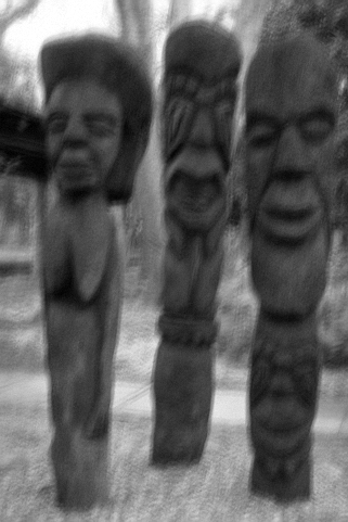
Non-blind deblurring. In this setting, $B$ is the matrix form of a convolution with a blur kernel. We use the experimental protocol of [52]: we blur the 68 test images of [29] with the two kernels of [23] and add $1\%$ Gaussian noise. We compare in Table 1 the proposed algorithms with the two variational methods of [23] (handcrafted prior on image gradients) and [52] (GMM prior on patches). Bold font indicates the best performer, and if marginally below, the second best too. For the MSE-based method, we set $\gamma=5000$ and for the $\ell_{2}$-based solvers, we set $\gamma=3200$, $\beta_{0}=3$, $\delta=2$ and $T=8$. For the two kernels, the $\ell_{2}$-based solver’s performance is on par with EPLL and outperforms HL by margins of about 1.5dB. Note that the MSE version of our solver does not do as well as EPLL and its $\ell_{2}$- version, and achieves similar results to the gradient-based prior of HL. It also shows that the choice of the loss, besides the kernel and computation of the $\alpha$, is an important aspect of our approach. An example is shown in Figure 2.

Table 1: Average PSNR for non-blind deblurring. The baselines are taken from [52].

Methods	HL [23]	EPLL [52]	Ours (MSE)	Ours ($\ell_{2}$)
Kernel 1 ($17\times 17$)	25.84	27.17	25.68	27.21
Kernel 2 ($19\times 19$)	26.38	27.70	26.31	27.96

Upsampling. We follow [41, 16] and implement $B$ as a convolution with an anti-aliasing Gaussian filter of standard deviation of 0.8, followed by decimation of factor 2. We evaluate our method in the test set Set5 used in [49], and compare it in Table 2 with bicubic interpolation and two variational methods specialized for upsampling; KSVD [49] and ANR [43] (dictionary learning-based). For the $\ell_{2}$-based solver, we set $\gamma=6000$, $\beta_{0}=0.5$, $\delta=2$, $T=3$. We obtain consistent better results than bicubic interpolation (+1.7dB) and slightly worse (-0.5dB) than specialized up-sampling methods KSVD and ANR. Note that we rely on simple DCT features and better results might be obtained with more adequate features. Due to a lack of space, qualitative results can be found in Appendix D.

Table 2: PSNRs for upsampling.

Methods	Bicubic	KSVD [49]	ANR [43]	Ours ($\ell_{2}$)
Baby	37.07	38.25	38.44	38.29
Bird	36.81	39.93	40.04	38.88
Butterfly	27.43	30.65	30.48	29.97
Head	34.86	35.59	35.66	35.63
Woman	32.14	34.49	34.55	34.03
Average	33.66	35.78	35.83	35.36

Other image restoration tasks. Denoising and inpainting are other local image restoration tasks where our framework can be applied to. In the case of denoising, the problem is less structured as the operator $B$ is the identity, so our method highly relies on the performance of the learned regularizers. We perform below standard methods such as [15, 13, 52] in classical benchmarks (see Appendix C). We think the main bottleneck is the data-driven regularizer: it is key to design kernels that are robust to large noise such as in [42, 7], and KRR may be needed instead of NW as the learning task is more important than the fitting term. We leave the task of fine-tuning our method for the specific problem of denoising for future work.

6 Conclusion

We have presented a new general framework for image restoration using localized structured prediction and non-linear multi-task learning that comes with statistical guarantees. We have implemented two settings using the Euclidean distance or its square as a loss, and demonstrated the effectiveness of our algorithms on several problems, achieving results comparable or better than existing variational methods. As a final note, we want to stress again the fact that our aim in this paper is not to obtain a new state of the art for the various image restoration tasks we have experimented with. Indeed, we are quite aware that some highly-tuned CNN architectures gave significantly higher performance for image denoising (e.g., [51]), non-blind deblurring (e.g., [50]), and upsampling (e.g., [14]). Our objective is instead to demonstrate that recent methods from the fields of structured prediction and non-linear multi-task learning with strong theoretical guarantees can effectively be adapted to image restoration problems, which we hope to have demonstrated with our experiments and comparisons with classical variational methods.

7 Broader impact

The main application of this paper is image restoration, with well known benefits (from personal photography and medical imaging to astronomy and microscopy) and risks (military and surveillance uses, and privacy issues related to deblurring images that were blurred to anonymize). These concerns are ubiquitous in machine learning in general and its applications to computer vision and image processing in particular, and beyond the scope of this presentation.

Aknowledgments.

This work was supported in part by the Inria/NYU collaboration and the Louis Vuitton/ENS chair on artificial intelligence. In addition, this work was funded in part by the French government under management of Agence Nationale de la Recherche as part of the “Investissements d’avenir” program, reference ANR19-P3IA-0001 (PRAIRIE 3IA Institute). ANV received support from La Caixa Fellowship.

Organization of the Appendix

• Theoretical Analysis of the Estimator
  Analysis of Section 3.

  • Derivation of the Estimator

  • Comparison Inequality

  • Generalization Bound

  • Assumptions on the Loss $\boldsymbol{\ell}$ and Target Distribution

• Algorithm
  Details of Section 4.

  • Convexity of the Energy

  • General Algorithms to Solve the $\boldsymbol{z_{p}}$ Update

  • SDCA for Euclidean Loss and Nadaraya-Watson Estimator

• Experiments
  Details of Section 5.

  • Analysis of the Constant $\boldsymbol{q}$

  • Implementation Details

  • Further Experiments

• Additional Images
  More visualizations.

Appendix A Theoretical Analysis of the Estimator

A.1 Derivation of the Estimator

Recall the goal is to estimate a function ${\bf x}:\mathcal{Y}\xrightarrow{}\mathcal{X}$ that minimizes the expected risk

$$\mathcal{E}({\bf x})=\operatorname{\mathbb{E}}_{(y,x)\sim\rho}~{}L({\bf x}(y),x),$$ (21)

under the constraint $\|y-B{\bf x}(y)\|_{2}^{2}\leq\sigma^{2}$, where the loss function $L$ decomposes by patches as

$$L(x,x^{\prime})=\frac{1}{|P|}\sum_{p\in P}\ell(x_{p},x_{p}^{\prime}).$$ (22)

In this subsection, we derive the proposed estimator of Eq. 10 from the risk minimization problem (2). More specifically, in Section A.1.1 we compute the form of the exact minimizer ${\bf x}_{\sigma}^{\star}$, in Section A.1.2, we describe the assumption on the loss function $\ell$ needed for the analysis, and in Section A.1.3 we use this decomposition to construct a quadratic surrogate, which provides the resulting estimator when minimized using kernel ridge regression.

A.1.1 Characterization of the optimum

Lemma A.1.

The minimizer ${\bf x}_{\sigma}^{\star}$ of the risk (21) under the constraint $\|y-B\widehat{\bf x}(y)\|_{2}^{2}\leq\sigma^{2}$ takes the form

$${\bf x}_{\sigma}^{\star}(y)\in\operatorname*{arg\;min}_{\|y-Bx\|_{2}^{2}\leq\sigma^{2}}\Omega_{L}^{\pi}(x~{}|~{}y),\quad\text{where}\quad\Omega_{L}^{\pi}(x~{}|~{}y)=\operatorname{\mathbb{E}}_{x^{\prime}\sim\pi_{y}}L(x,x^{\prime}),$$ (23)

where $\pi_{y}(x)=\rho(x~{}|~{}y)$ denotes the conditional distribution of $x$ given $y$.

Proof.

We first show that the problem can be solved independently for every $y\in\mathcal{Y}$.

$${\bf x}_{\sigma}^{\star}=\underset{\begin{subarray}{c}{\bf x}:\mathcal{Y}\xrightarrow{}\mathcal{X}\\ \|y-B{\bf x}(y)\|_{2}^{2}\leq\sigma^{2}\end{subarray}}{\operatorname{argmin}}\operatorname{\mathbb{E}}_{(y,x)\sim\rho}L({\bf x}(y),x)=\underset{\begin{subarray}{c}{\bf x}:\mathcal{Y}\xrightarrow{}\mathcal{X}\\ \|y-B{\bf x}(y)\|_{2}^{2}\leq\sigma^{2}\end{subarray}}{\operatorname{argmin}}\operatorname{\mathbb{E}}_{x\sim\rho_{\mathcal{X}}}\operatorname{\mathbb{E}}_{x\sim\pi_{y}}L({\bf x}(y),x),$$ (24)

where $\rho_{\mathcal{X}}$ denotes the marginal distribution in $\mathcal{X}$. Hence, the problem decouples in $y$ and one can write

$${\bf x}_{\sigma}^{\star}(y)=\operatorname*{arg\;min}_{\begin{subarray}{c}x\in\mathcal{X}\\ \|y-Bx\|_{2}^{2}\leq\sigma^{2}\end{subarray}}~{}\operatorname{\mathbb{E}}_{x^{\prime}\sim\pi_{y}}L(x,x^{\prime}).$$

See Lemma 6 of [10] for the full proof (taking into account also measure theoretic aspects). ∎

For the rest of the Appendix, we assume that between-locality (introduced in Section 2.1) holds. We recall here the assumption:

• The sharp patch $x_{p}$ is conditionally independent from $y$ given $y_{p}$.

• The following holds for all patches $p,p^{\prime}\in P$,

  $$\pi_{y_{p}}(x_{p})=\pi_{y_{p^{\prime}}}(x_{p^{\prime}})$$ (25)

In particular, this allows us to write

$$\Omega_{L}^{\pi}(x~{}|~{}y)=\frac{1}{|P|}\sum_{p\in P}\Omega_{\ell}^{\pi}(x_{p}~{}|~{}y_{p}),\quad\textrm{where},\quad\Omega_{\ell}^{\pi}(\text{x}~{}|~{}\text{y})=\operatorname{\mathbb{E}}_{\text{x}^{\prime}\sim\pi_{\text{y}}}\ell(\text{x},\text{x}^{\prime}).$$ (26)

A.1.2 Decomposition of the loss

In order to derive the estimator and to proceed further with the theoretical analysis, we need to introduce a mild assumption on the loss $\ell$ at the patch level.

SELF assumption of the loss $\boldsymbol{\ell}$. There exists a separable Hilbert space $\mathcal{H}$ and continuous bounded maps $\psi,\varphi:[\mathcal{X}]\xrightarrow{}\mathcal{H}$ such that the loss function $\ell$ between sharp image patches decomposes as:

$$\ell(\text{x},\text{x}^{\prime})=\langle\psi(\text{x}),\varphi(\text{x}^{\prime})\rangle_{\mathcal{H}},$$ (27)

for all $\text{x},\text{x}^{\prime}\in[\mathcal{X}]$.

In particular, it was shown by [10] (see Thm. 19) that the above assumption holds if the loss function $\ell$ is absolutely continuous and $[\mathcal{X}]$ is a compact space, which is our case. Moreover, note that the assumption is always satisfied when the spaces are discrete, as Eq. 27 corresponds to a low-rank decomposition of the loss matrices. In Section A.4 we study the SELF assumption more explicitly under the hypothesis of the loss from our main Theorem 3.1.

A.1.3 Construction of the quadratic surrogate

Notation.

In this subsection we are going to use a construction widely used in the context of quadratic surrogate approaches for structured prediction, with the goal of deriving the estimator in Eq. 10 (for more details on this kind of construction see [11]). The assumption (27) on the loss functions allows us to write the exact minimizer ${\bf x}_{\sigma}^{\star}$ with respect to the functions $g^{\star}:[\mathcal{Y}]\xrightarrow{}\mathcal{H}$ defined as the conditional expectation of the embedding $\varphi$:

$$g^{\star}(\text{y})=\operatorname{\mathbb{E}}_{\text{x}\sim\pi_{\text{y}}}\varphi(\text{x}).$$ (28)

This can be seen by simply moving the conditional expectation inside the scalar product as:

$${\bf x}_{\sigma}^{\star}(y) \in\operatorname*{arg\;min}_{\begin{subarray}{c}x\in\mathcal{X}\\ \|y-Bx\|_{2}^{2}\leq\sigma^{2}\end{subarray}}~{}\Omega_{L}^{\pi}(x~{}|~{}y)$$

$$=\operatorname*{arg\;min}_{\begin{subarray}{c}x\in\mathcal{X}\\ \|y-Bx\|_{2}^{2}\leq\sigma^{2}\end{subarray}}~{}\frac{1}{|P|}\sum_{p\in P}\Omega_{\ell}^{\pi}(x_{p}~{}|~{}y_{p})$$

$$=\operatorname*{arg\;min}_{\begin{subarray}{c}x\in\mathcal{X}\\ \|y-Bx\|_{2}^{2}\leq\sigma^{2}\end{subarray}}~{}\frac{1}{|P|}\sum_{p\in P}\operatorname{\mathbb{E}}_{x_{p}^{\prime}\sim\pi_{y_{p}}}\langle\psi(x_{p}),\varphi(x_{p}^{\prime})\rangle_{\mathcal{H}}$$

$$=\operatorname*{arg\;min}_{\begin{subarray}{c}x\in\mathcal{X}\\ \|y-Bx\|_{2}^{2}\leq\sigma^{2}\end{subarray}}~{}\frac{1}{|P|}\sum_{p\in P}\langle\psi(x_{p}),g^{\star}(y_{p})\rangle_{\mathcal{H}}$$

A natural strategy for building an approximator $\widehat{\bf x}$ of ${\bf x}_{\sigma}^{\star}$ is to design an estimator $\widehat{g}$ of $g^{\star}$ and consider:

$$\widehat{\bf x}(y)\in\operatorname*{arg\;min}_{\|y-Bx\|_{2}^{2}\leq\sigma^{2}}~{}\frac{1}{|P|}\sum_{p\in P}\langle\psi(x_{p}),\widehat{g}(y_{p})\rangle_{\mathcal{H}}.$$ (29)

The question now boils down to constructing the estimator $\widehat{g}$. The important observation is that as $g^{\star}$ is written as a conditional expectation, it is characterized as the minimum of the expected squared error measured in the Hilbert space $\mathcal{H}$:

$$g^{\star}=\operatorname*{arg\;min}_{g:[\mathcal{Y}]\xrightarrow{}\mathcal{H}}~{}\operatorname{\mathbb{E}}_{(\text{y},\text{x})\sim\rho}\|\varphi(\text{x})-g(\text{y})\|_{\mathcal{H}}^{2},$$ (30)

where now $\rho$ denotes the distribution over patches instead of full images. Given a dataset of patches $(\text{y}^{(i)},\text{x}^{(i)})_{1\leq i\leq m}$, we can approximate the minimizers of Eq. 30 with kernel ridge regression as:

$$\widehat{g}=\operatorname*{arg\;min}_{g\in\mathcal{G}\otimes\mathcal{H}}\frac{1}{m}\sum_{j=1}^{m}\|\varphi(\text{x}^{(i)})-g(\text{y}^{(i)})\|_{\mathcal{H}}^{2}+\lambda\|g\|_{\mathcal{G}\otimes\mathcal{H}}^{2},$$ (31)

where $\mathcal{G}$ is the scalar reproducing kernel Hilbert space (RKHS) associated to the positive definite kernel $k:[\mathcal{Y}]\times[\mathcal{Y}]\xrightarrow{}\mathbb{R}$, $\mathcal{G}\otimes\mathcal{H}$ denotes the vector-valued RKHS corresponding to the tensor product between $\mathcal{G}$ and $\mathcal{H}$, and $\lambda>0$ is a regularization parameter. The solution of Eq. 31 can be computed in closed form as:

$$\widehat{g}(\text{y})=\sum_{i=1}^{m}\alpha_{i}(\text{y})\varphi(\text{x}^{(i)}),$$ (32)

where $\alpha(\text{y})$ is defined as:

$$\alpha(\text{y})=(K+m\lambda I)^{-1}v(\text{y})\in\mathbb{R}^{m},$$ (33)

where $v(\text{y})$ is a vector in $\mathbb{R}^{m}$ with $i$-th component $k(\text{y},\text{y}^{(i)})$ and $K$ is a matrix in $\mathbb{R}^{m\times m}$ defined by $K(i,j)~{}=~{}k(\text{y}^{(i)},\text{y}^{(j)})$.

Using the linearity of the scalar product and the fact that $\widehat{g}$ is linear in the embeddings $\varphi$ evaluated at training data points of sharp image patches, we obtain that the estimators $\widehat{\Omega}_{\ell}^{\pi}$ are independent of the embeddings (27) of the loss function $\ell$:

$$\widehat{\Omega}_{\ell}^{\pi}(x_{p}~{}|~{}y_{p})=\langle\psi(x_{p}),\widehat{g}(y_{p})\rangle_{\mathcal{H}}=\sum_{i=1}^{m}\alpha_{i}(y_{p})\langle\psi(x_{p}),\varphi(\text{y}^{(i)})\rangle_{\mathcal{H}}=\sum_{i=1}^{m}\alpha_{i}(y_{p})\ell(x_{p},\text{x}^{(i)}).$$ (34)

A.2 Comparison Inequality

In Section A.1, we have derived $\widehat{\bf x}$ by estimating a vector-valued function $g^{\star}$ taking values in a Hilbert space $\mathcal{H}$ defined by the decomposition of the loss functions in Eq. 27. The goal of this section, is to analyze how the error of estimating $g^{\star}$ by $\widehat{g}$ translates to the excess risk $\mathcal{E}(\widehat{\bf x})-\mathcal{E}({\bf x}_{\sigma}^{\star})$, which is the quantity that we ultimately want to bound. This quantification is made precise by the following Theorem A.2, which is analogous to Thm. 9 by [9] but with a more careful analysis of the constants in order to make appear the effect of the constraint $\|y-B{\bf x}(y)\|_{2}^{2}\leq\sigma^{2}$.

Notation.

Let’s first define $G(y)=g(y_{p})_{p\in P}$ and $\Psi(x)=\psi(x_{p})_{p\in P}$, so that

$$\langle\Psi(x),G(y)\rangle_{\mathcal{H}_{P}}=\frac{1}{|P|}\sum_{p\in P}\langle\psi(x_{p}),g(y_{p})\rangle_{\mathcal{H}},$$ (35)

where $\mathcal{H}_{P}=\bigoplus_{p\in P}\mathcal{H}$ is the direct sum of $|P|$ copies of $\mathcal{H}$. t the last step, we used the fact that $\|y-B\widehat{x}(y)\|_{2}^{2}\leq\sigma^{2}$ and

Theorem A.2 (Comparison inequality).

Assume that $\ell$ satisfies (27). Let $\widehat{\bf x}$ and ${\bf x}_{\sigma}^{\star}$ be defined in Eq. 29 and Eq. 23, respectively. Then,

$$\mathcal{E}(\widehat{\bf x})-\mathcal{E}({\bf x}_{\sigma}^{\star})\leq 2c_{B,\sigma}^{1/2}\big{(}\operatorname{\mathbb{E}}_{y\sim\rho_{\mathcal{Y}}}\|\widehat{G}(y)-G^{\star}(y)\|_{\mathcal{H}_{P}}^{2}\big{)}^{1/2},$$ (36)

where $\rho_{\mathcal{Y}}$ denotes the marginal distribution in $\mathcal{Y}$ and

$$c_{B,\sigma}=\operatorname{\mathbb{E}}_{y\sim\rho_{\mathcal{Y}}}\operatorname{diam}^{2}(\Psi(\mathcal{C}_{B,\sigma}(y))),$$ (37)

with $\mathcal{C}_{B,\sigma}(y)=\{x\in\mathcal{X}~{}|~{}\|Bx-y\|_{2}\leq\sigma\}$.

Proof.

We have that

$$\mathcal{E}(\widehat{\bf x}) -\mathcal{E}({\bf x}_{\sigma}^{\star})\leq\operatorname{\mathbb{E}}_{y\sim\rho_{\mathcal{Y}}}\langle\Psi(\widehat{\bf x}(y)),G^{\star}(y)\rangle-\langle\Psi({\bf x}_{\sigma}^{\star}(y)),G^{\star}(y)\rangle$$

$$=\operatorname{\mathbb{E}}_{y\sim\rho_{\mathcal{Y}}}\langle\Psi(\widehat{\bf x}(y)),G^{\star}(y)-\widehat{G}(y)\rangle+\underbrace{\langle\Psi(\widehat{\bf x}(y))-\Psi({\bf x}_{\sigma}^{\star}(y),\widehat{G}(y)\rangle}_{\leq 0}$$

$$+\operatorname{\mathbb{E}}_{y\sim\rho_{\mathcal{Y}}}\langle\Psi({\bf x}_{\sigma}^{\star}(y)),\widehat{G}(y)-G^{\star}(y)\rangle$$

$$=\operatorname{\mathbb{E}}_{y\sim\rho_{\mathcal{Y}}}\langle\Psi(\widehat{\bf x}(y)),G^{\star}(y)-\widehat{G}(y)\rangle+\langle\Psi({\bf x}_{\sigma}^{\star}(y)),\widehat{G}(y)-G^{\star}(y)\rangle$$

$$=\operatorname{\mathbb{E}}_{y\sim\rho_{\mathcal{Y}}}\min_{v\in\mathcal{H}_{P}}\big{(}\langle\Psi(\widehat{\bf x}(y))-v,G^{\star}(y)-\widehat{G}(y)\rangle+\langle\Psi({\bf x}_{\sigma}^{\star}(y))-v,\widehat{G}(y)-G^{\star}(y)\rangle\big{)}$$

$$\leq\operatorname{\mathbb{E}}_{y\sim\rho_{\mathcal{Y}}}\sup_{x,x^{\prime}\in\mathcal{C}_{B,\sigma}(y)}\min_{v\in\mathcal{H}_{P}}\big{(}\langle\Psi(\widehat{\bf x}(y))-v,G^{\star}(y)-\widehat{G}(y)\rangle+\langle\Psi({\bf x}_{\sigma}^{\star}(y))-v,\widehat{G}(y)-G^{\star}(y)\rangle\big{)}$$

$$\leq\operatorname{\mathbb{E}}_{y\sim\rho_{\mathcal{Y}}}\sup_{x,x^{\prime}\in\mathcal{C}_{B,\sigma}(y)}\min_{v\in\mathcal{H}_{P}}(\|\Psi(x)-v\|_{\mathcal{H}_{P}}+\|\Psi(x^{\prime})-v\|_{\mathcal{H}_{P}})\|G^{\star}(y)-\widehat{G}(y)\|$$

$$\leq\operatorname{\mathbb{E}}_{y\sim\rho_{\mathcal{Y}}}\sup_{x,x^{\prime}\in\mathcal{C}_{B,\sigma}(y)}\|\Psi(x)-\Psi(x^{\prime})\|_{\mathcal{H}_{P}}\|G^{\star}(y)-\widehat{G}(y)\|_{\mathcal{H}_{P}}$$

$$=\operatorname{\mathbb{E}}_{y\sim\rho_{\mathcal{Y}}}\operatorname{diam}(\Psi(\mathcal{C}_{B,\sigma}(y)))\|G^{\star}(y)-\widehat{G}(y)\|_{\mathcal{H}_{P}}$$

$$\leq\sqrt{\operatorname{\mathbb{E}}_{y\sim\rho_{\mathcal{Y}}}\operatorname{diam}^{2}(\Psi(\mathcal{C}_{B,\sigma}(y)))~{}\times~{}\operatorname{\mathbb{E}}_{y\sim\rho_{\mathcal{Y}}}\|G^{\star}(y)-\widehat{G}(y)\|^{2}},$$

where we have used that $\min_{v\in\mathcal{H}}~{}\|u-v\|_{\mathcal{H}}+\|u^{\prime}-v\|_{\mathcal{H}}=\|u-u^{\prime}\|_{\mathcal{H}}$ if $\mathcal{H}$ is a Hilbert space. ∎

Theorem A.3 (Constant $c_{B,\sigma}$).

Under the hypothesis on $\ell$ from Theorem 3.1, the constant $c_{B,\sigma}$ is bounded as

$$c_{B,\sigma}\leq\operatorname{diam}([\mathcal{X}])\frac{\operatorname{\mathbb{E}}_{y\sim\rho_{\mathcal{Y}}}\operatorname{diam}(\mathcal{C}_{B,\sigma}(y))}{\operatorname{diam}(\mathcal{X})}.$$ (38)

Proof.

Let $c_{B,\sigma}=\operatorname{\mathbb{E}}_{y\sim\rho_{\mathcal{Y}}}c_{B,\sigma}(y)$, where

$$c_{B,\sigma}(y)=\operatorname{diam}^{2}(\Psi(\mathcal{C}_{B,\sigma}(y)))=\sup_{x,x^{\prime}\in\mathcal{C}_{B,\sigma}(y)}\big{\|}\Psi(x)-\Psi(x^{\prime})\big{\|}_{\mathcal{H}_{P}}^{2}.$$ (39)

Using the hypothesis on $\ell$ from Theorem 3.1 and Lemma A.6, we can write $\langle\psi(x_{p}),\psi(x_{p}^{\prime})\rangle_{\mathcal{H}}=e^{-\|x_{p}-x_{p}^{\prime}\|_{2}}$. Hence, the squared distance between embeddings $\psi$ takes the form $\|\psi(x_{p})-\psi(x_{p}^{\prime})\|_{\mathcal{H}}^{2}=1-e^{-\|x_{p}-x_{p}^{\prime}\|_{2}}$. We have that $c_{B,\sigma}^{2}=\operatorname{\mathbb{E}}_{y\sim\rho_{\mathcal{Y}}}c_{B,\sigma}(y)^{2}$, where

$$c_{B,\sigma}(y) =\sup_{x,x^{\prime}\in\mathcal{C}_{B,\sigma}(y)}\big{\|}\Psi(x)-\Psi(x^{\prime})\big{\|}_{\mathcal{H}_{P}}^{2}$$ (40)

$$=\sup_{x,x^{\prime}\in\mathcal{C}_{B,\sigma}(y)}\frac{1}{|P|}\sum_{p\in P}\|\psi(x_{p})-\psi(x_{p}^{\prime})\|_{\mathcal{H}}^{2}$$ (41)

$$=\sup_{x,x^{\prime}\in\mathcal{C}_{B,\sigma}(y)}\frac{1}{|P|}\sum_{p\in P}1-e^{-\|x_{p}-x_{p}^{\prime}\|_{2}}$$ (42)

$$\leq\sup_{x,x^{\prime}\in\mathcal{C}_{B,\sigma}(y)}\frac{1}{|P|}\sum_{p\in P}\|x_{p}-x_{p}^{\prime}\|_{2}$$ (43)

$$\leq\Big{(}\sup_{x,x^{\prime}\in\mathcal{C}_{B,\sigma}(y)}\frac{1}{|P|}\sum_{p\in P}\|x_{p}-x_{p}^{\prime}\|_{2}^{2}\Big{)}^{1/2}$$ (44)

$$=\frac{C^{1/2}}{|P|^{1/2}}\Big{(}\sup_{x,x^{\prime}\in\mathcal{C}_{B,\sigma}(y)}\|x-x^{\prime}\|_{2}^{2}\Big{)}^{1/2}$$ (45)

$$=\frac{C^{1/2}}{|P|^{1/2}}\sup_{x,x^{\prime}\in\mathcal{C}_{B,\sigma}(y)}\|x-x^{\prime}\|_{2}$$ (46)

$$=\frac{C^{1/2}}{|P|^{1/2}}\operatorname{diam}(\mathcal{C}_{B,\sigma}(y)),$$ (47)

where we have used that $\sum_{p\in P}\|x_{p}-x_{p}^{\prime}\|_{2}^{2}=C\|x-x^{\prime}\|_{2}^{2}$, where $C$ is the number of patches a pixel belongs to. Using that $\operatorname{diam}([\mathcal{X}])^{2}=\frac{C}{|P|}\operatorname{diam}(\mathcal{X})^{2}$, we obtain

$$c_{B,\sigma}(y)\leq\operatorname{diam}([\mathcal{X}])\frac{\operatorname{diam}(\mathcal{C}_{B,\sigma}(y))}{\operatorname{diam}(\mathcal{X})}.$$ (48)

Taking the expectation w.r.t $y$ in both sides we obtain the desired result. ∎

In the following Proposition A.4, we compute explicitly an upper bound of the constant $c_{B,\sigma}$ for the tasks of denoising, inpainting and downsampling.

Proposition A.4 (Bounding $c_{B,\sigma}$ for specific problems).

The constant $c_{B,\sigma}$ can bounded explicitly for the following settings.

• Denoising. The degradation model is $y=x+\varepsilon$. Hence, $B=Id$ and $\sigma>0$. The constant takes the following form

  $$c_{B,\sigma}\propto\min\left(\frac{\sigma}{\operatorname{diam}(\mathcal{X})},1\right)$$ (49)

• Inpainting. The operator $B$ is a the identity matrix with a ratio of $s$ zeros in the diagonal. If we assume there is no noise, the constant takes the following form

  $$c_{B,\sigma}\propto s^{1/2}.$$ (50)

• Downsampling. The operator $B$ is the downsampling operator by a factor of $k$. If we assume there is no noise, the constant takes the following form

  $$c_{B,\sigma}\propto k^{-1/2}.$$ (51)

Proof.

We proceed separately for every setting. Note that the space of sharp images is the cube $\mathcal{X}=[0,1]^{d}$ where $d$ is the total number of pixels.

• Denoising. The set $\mathcal{C}_{B,\sigma}(y)$ is an $\ell_{2}$ ball centered at $y$ with radius $\sigma$ intersected with the cube $\mathcal{X}$. Hence, it directly follows $\operatorname{diam}(\mathcal{C}_{B,\sigma}(y))\leq\sigma$.

• Inpainting. The set $\mathcal{C}_{B,\sigma}(y)$ is a cube centered at $y$ of dimension $ds$. Using that the diameter of a cube of dimension $d$ is $\sqrt{d}$, we obtain that $\operatorname{diam}(\mathcal{C}_{B,\sigma}(y))/\operatorname{diam}(\mathcal{X})\leq\sqrt{\frac{ds}{d}}=s^{1/2}$.

• Downsampling. The set $\mathcal{C}_{B,\sigma}(y)$ is a cube centered at $y$ of dimension $d/k$, using the expression of the diameter of the cube as before, we obtain $\operatorname{diam}(\mathcal{C}_{B,\sigma}(y))/\operatorname{diam}(\mathcal{X})\leq\sqrt{\frac{d/k}{d}}=\sqrt{1/k}$.

∎

A.3 Generalization Bound

The goal of this section is to prove Theorem 3.1 by first bounding the estimation error of the surrogate problem $\operatorname{\mathbb{E}}_{y\sim\rho_{\mathcal{Y}}}\|G^{\star}(y)-\widehat{G}(y)\|_{\mathcal{H}_{P}}^{2}$ and applying the comparison inequality derived in Theorem A.2. Define the quantities $\mathsf{g},r,q$ as:

$$\mathsf{g}=\|g^{\star}\|_{\mathcal{G}\otimes\mathcal{H}},\hskip 14.22636ptr=\sup_{\text{y}\in[\mathcal{Y}]}k(\text{y},\text{y}),$$ (52)

$$q=\frac{1}{|P|r^{2}}\sum_{p,p^{\prime}\in P}\operatorname{\mathbb{E}}_{y,y^{\prime}}C_{p,p^{\prime}}(y,y^{\prime}),\hskip 14.22636ptC_{p,p^{\prime}}(y,y^{\prime})=k(y_{p},y_{p^{\prime}})^{2}-k(y_{p},y_{p^{\prime}}^{\prime})^{2}.$$ (53)

We have the following theorem.

Theorem A.5 (Generalization bound).

Assume that the decomposition of the loss $\ell$ in Eq. 27 holds and $\mathsf{g}<+\infty$. Moreover, assume between-locality and let the regularization parameter of KRR be

$$\lambda=r\sqrt{\frac{1}{m}+\frac{q}{|P|n}}.$$ (54)

Then, we have that:

$$\operatorname{\mathbb{E}}\mathcal{E}(\widehat{\bf x})-\mathcal{E}({\bf x}_{\sigma}^{\star})\leq 12c_{B,\sigma}^{1/2}r^{1/2}\mathsf{g}\left(\frac{1}{m}+\frac{1+q}{|P|n}\right)^{1/4},$$ (55)

where the first expectation is taken over the $m$ realizations of the dataset of patches $(\text{y}^{(i)},\text{x}^{(i)})_{1\leq i\leq m}$.

Proof.

The result corresponds to Thm. 4 of [9] where in the proof we used our comparison inequality (36) instead of theirs. ∎

In order to prove our main result (Theorem 3.1), we now show that the assumptions on the loss $\ell$ and the target distribution appearing in Section 3 imply the assumptions made in Theorem A.5.

A.4 Assumptions on the Loss $\boldsymbol{\ell}$ and Target Distribution

We recall here the assumption on the smoothness on $\ell$ and $\rho$ and derive some implications that will be useful to prove Theorem 3.1. Let the set of patches be defined respectively as $[\mathcal{X}]=[-1,1]^{d_{\mathcal{X}}\times d_{\mathcal{X}}}$ and $[\mathcal{Y}]=\mathbb{R}^{d_{\mathcal{Y}}\times d_{\mathcal{Y}}}$, with $d_{\mathcal{X}},d_{\mathcal{Y}}\in\mathbb{N}$. Denote by $W^{s}_{2}(Z)$ the Sobolev space of smoothness $s>0$ in a set $Z$, i.e. the space of functions with square-integrable weak derivatives up to order $s$ [2].

Assumption on the loss $\boldsymbol{\ell}$. There exists $C\in(0,\infty),s\geq\frac{d_{\mathcal{X}}^{2}+1}{2}$ s.t. $\sup_{\text{x}\in[\mathcal{X}]}\|\ell(\cdot,\text{x})\|_{W^{s}_{2}([\mathcal{X}])}\leq C$.

Lemma A.6.

Under the assumption above, $\ell$ satisfies the SELF assumption with $\mathcal{H}$ = $W^{p}_{2}([\mathcal{X}])$, with $p=\frac{d_{\mathcal{X}}^{2}+1}{2}$ and $\psi$ be the feature map associated to the Abel kernel, i.e., $\left\langle\psi(\text{x}),\psi(\text{x}^{\prime})\right\rangle_{\mathcal{H}}=e^{-\|\text{x}-\text{x}^{\prime}\|}$.

Proof.

Since $s\geq p$, we have $W^{s}_{2}([\mathcal{X}])\subseteq W^{p}_{2}([\mathcal{X}])$ [2]. By Theorem 8 point (c) [11] and the assumption on $\ell$, we have that there exists a uniformly bounded measurable feature map $\varphi$, such that $\ell(\text{x},\text{x}^{\prime})=\left\langle\psi(\text{x}),\varphi(\text{x}^{\prime})\right\rangle_{\mathcal{H}}$, with $\mathcal{H}=W^{p}_{2}([\mathcal{X}])$. ∎

Assumption on the target distribution. Let $m\in\mathbb{N}$ s.t. $W^{m}_{2}([\mathcal{Y}])\subseteq{\mathcal{H}}$ where $\mathcal{H}$ is the reproducing kernel Hilbert space associated to the kernel $k$ [3, 4]. For example, $m=d_{\mathcal{Y}}^{2}/2+1$ for the Laplacian kernel $k(\text{y},\text{y}^{\prime})=e^{-\|\text{y}-\text{y}^{\prime}\|}$. We require $\rho(\text{x}|\text{y})$ to be density and satisfy $\rho(\text{x}|\text{y})\in W^{m}_{2}([\mathcal{X}]\times[\mathcal{Y}]).$

Lemma A.7.

Under the assumption above on $\rho$ and $k$ we have $\|g^{\star}\|_{{\cal G}\otimes{\cal H}}<\infty$.

Proof.

Note that by the SELF condition, $g^{\star}=\int\varphi(\text{x})d\rho(\text{x}|\text{y})$, where $\varphi:[\mathcal{X}]\to{\cal H}$ is a uniformly bounded measurable map and ${\cal H}$ a separable Hilbert space defined in the proof of the lemma above. Note moreover, that since $\rho\in W^{m}_{2}(\mathcal{X}\times\mathcal{Y}),$ and $W^{m}_{2}(\mathcal{X}\times\mathcal{Y})\subseteq W^{m}_{2}(\mathcal{X})\otimes W^{m}_{2}(\mathcal{Y})$ [2]. Finally note that $W^{m}_{2}(\mathcal{X})\otimes W^{m}_{2}(\mathcal{Y})\subseteq W^{m}_{2}(\mathcal{X})\otimes{\cal G}$ since $W^{m}_{2}(\mathcal{Y})\subseteq{\cal G}$ by assumption. Since $\rho\in W^{m}_{2}(\mathcal{X})\otimes{\cal G}$, then there exists a Hilbert-Schmidt operator $R:{\cal G}\to W^{m}_{2}(\mathcal{X})$ such that $\rho(\text{x}|\text{y})=\left\langle h_{\mathcal{X}}(\text{x}),Rh_{\mathcal{Y}}(\text{y})\right\rangle_{W^{m}_{2}(\mathcal{X})}$, where $h_{\mathcal{Y}}:[\mathcal{Y}]\to{\cal G}$ is the uniformly bounded continuous feature map associated to the kernel $k$ and $h_{\mathcal{X}}:[\mathcal{X}]\to W^{m}_{2}(\mathcal{X})$ is the uniformly bounded continuous feature map associated to the canonical kernel of $W^{m}_{2}(\mathcal{X})$. Now note that by construction $\rho$ is a density and so, for all $\text{y}\in[\mathcal{Y}]$, we have

$$g^{\star}(\text{y}) =\int_{\mathcal{X}}\varphi(\text{x})\left\langle h_{\mathcal{X}}(\text{x}),Rh_{\mathcal{Y}}(\text{y})\right\rangle_{W^{m}_{2}(\mathcal{X})}d\text{x}$$

$$=\left(\int_{\mathcal{X}}\varphi(\text{x})\otimes h_{\mathcal{X}}(\text{x})d\text{x}\right)~{}R~{}h_{\mathcal{Y}}(\text{y})=~{}~{}g^{\star}h_{\mathcal{Y}}(\text{y}),$$

where $g^{\star}=HR$, with $H:W^{m}_{2}(\mathcal{X})\to{\cal H}$ is a linear operator defined as $H=\int_{\mathcal{X}}\varphi(\text{x})\otimes h_{\mathcal{X}}(\text{x})d\text{x}$. Now note that $H$ is trace class, since both $\varphi,h_{\mathcal{X}}$ are uniformly bounded and $\mathcal{X}$ is compact. Since $R$ is a Hilbert-Schmidt opertator, then $\|g^{\star}\|_{HS}\leq\|H\|_{op}\|R\|_{HS}\leq\|g^{\star}\|_{HS}\leq\|H\|_{tr}\|R\|_{HS}<\infty$. The proof is concluded by considering the isomorphism between the Hilbert space ${\cal G}\otimes{\cal H}$ and the space of Hilbert-Schmidt operators between ${\cal G}$ and ${\cal H}$, since we have already proved that $g^{\star}(\text{y})=g^{\star}h_{\mathcal{Y}}(\text{y})$, for all $y\in[\mathcal{Y}]$, with $g^{\star}$ a Hilbert-Schmidt operator. ∎

Proof of Theorem 3.1.

By Lemma A.6 and Lemma A.7 we first prove that the assumptions on $\ell$ and on $\rho$ satisfy the requirements on Theorem A.5 and then we apply Theorem A.5.

Appendix B Algorithm

In this section we discuss the algorithmic aspects of our estimator. In Section B.1 we study the convexity of the energy when the $\alpha$’s are computed using kernel ridge regression (KRR) and the Nadaraya-Watson (NW) estimator. In Section B.2 we expose linearly convergent methods to solve the $z_{p}$ update (18) and in Section B.3 we derive SDCA with gap sampling for the case when the $\alpha$’s are computed using the NW estimator and the loss $\ell$ is the Euclidean loss.

B.1 Convexity of the Energy

For the convexity analysis, we will assume for simplicity that $q\approx 0$, which means that there is small correlation between the patches of the degraded image. This is further justified in Section C.1.

We study the convexity of the energy of the $z_{p}$ update (18):

$$\sum_{i=1}^{m}\alpha_{i}(\text{y})\ell(\text{z},\text{x}^{(i)})+\beta/2\|\text{z}-\text{x}\|_{2}^{2},$$ (56)

when $\ell$ is convex in its first argument, where for the sake of exposition, we have defined $\text{y}=y_{p}$, $\text{z}\mathrel{\vbox{\hbox{\scriptsize.}\hbox{\scriptsize.}}}=z_{p}$ and $\text{x}=x_{p}$. In the case where the $\alpha$’s are computed using the Nadaraya-Watson (NW) estimator, all the coefficients are positive, and so (56) is convex because $\alpha_{i}(\text{y})\ell(\text{z},\text{x}^{(i)})$ remain convex. Unfortunately, some coefficients may be non-positive when the $\alpha$’s are computed using kernel ridge regression (KRR). The goal of the following Theorem B.1 is to show that in this case, in expectation the energy is also convex.

Theorem B.1 (Convexity of the energy).

Assume that the loss $\ell$ is two-times (absolutely) continuously differentiable in the first argument and the target distribution satisfies the same assumption as in Theorem 3.1. Let $\lambda=rm^{-1/2}$. If $\ell$ is convex in the first argument, there exists $m^{\prime}\in\mathbb{N}$ such that

$$\operatorname{\mathbb{E}}~{}\operatorname{\mathbb{E}}_{\text{y}\sim\rho_{\mathcal{Y}}}\sum_{i=1}^{m}\alpha_{i}(\text{y})\ell(\text{z},\text{x}^{(i)})+\beta/2\|\text{z}-\text{x}\|_{2}^{2},$$ (57)

is convex in $z\in[\mathcal{X}]$ for all $m\geq m^{\prime}$, where the first expectation is taken over the $m$ realizations of the dataset of patches.

Proof.

Let $\ell_{jk}(\text{x},\text{x}^{\prime})$ be the $j,k$-crossed-derivatives of the loss $\ell$ in the first argument. From [10] (see Thm. 19), we know that if $\ell_{jk}(\text{x},\text{x}^{\prime})$ is absolutely continuous, then the SELF assumption (27) is satisfied and we can write

$$\ell_{jk}(\text{x},\text{x}^{\prime})=\langle\psi_{jk}(\text{x}),\varphi_{jk}(\text{x}^{\prime})\rangle_{\mathcal{H}_{jk}}.$$

for continuous mappings $\psi_{jk},\varphi_{jk}:[\mathcal{X}]\rightarrow\mathcal{H}_{jk}$ and separable Hilbert space $\mathcal{H}_{jk}$. Let us now define $H_{\text{z}}(\text{y})$ and $\widehat{H}_{\text{z}}(\text{y})$ to be the Hessians of $\text{z}\mapsto\operatorname{\mathbb{E}}_{\text{x}^{\prime}\sim\pi_{\text{y}}}\ell(\text{z},\text{x}^{\prime})$ and $\text{z}\mapsto\sum_{i=1}^{m}\alpha_{i}(\text{y})\ell(\text{z},\text{x}^{(i)})$. If we denote $g_{jk}^{\star}(\text{y})=\operatorname{\mathbb{E}}_{\text{x}^{\prime}\sim\rho_{\text{y}}}\varphi_{jk}(\text{x}^{\prime})$ and $\widehat{g}_{jk}(\text{y})=\sum_{i=1}^{m}\alpha_{i}(\text{y})\varphi_{jk}(\text{x}^{(i)})$, we have that

$$\sup_{\text{z}\in[\mathcal{X}]}\operatorname{\mathbb{E}}\operatorname{\mathbb{E}}_{\text{y}}(\widehat{H}_{\text{z}}^{jk}(\text{y})-H_{\text{z}}^{jk}(\text{y}))^{2} =\sup_{\text{z}\in[\mathcal{X}]}\operatorname{\mathbb{E}}\operatorname{\mathbb{E}}_{\text{y}}\big{(}\langle\psi_{jk}(\text{z}),\widehat{g}_{jk}(\text{y})-g^{\star}_{jk}(\text{y})\rangle_{\mathcal{H}_{jk}}\big{)}^{2}$$ (58)

$$\leq\sup_{\text{z}\in[\mathcal{X}]}\|\psi_{jk}(\text{z})\|_{\mathcal{H}_{jk}}^{2}\operatorname{\mathbb{E}}\operatorname{\mathbb{E}}_{\text{y}}\|\widehat{g}_{jk}(\text{y})-g^{\star}_{jk}(\text{y})\|_{\mathcal{H}_{jk}}^{2}$$ (59)

$$\leq\sup_{\text{z}\in[\mathcal{X}]}C\|\psi_{jk}(\text{z})\|_{\mathcal{H}_{jk}}^{2}\|g_{jk}^{\star}\|_{\mathcal{G}\otimes\mathcal{H}_{jk}}^{2}m^{-1/2}$$ (60)

$$=C^{\prime}\|g_{jk}^{\star}\|_{\mathcal{G}\otimes\mathcal{H}_{jk}}^{2}m^{-1/2}.$$ (61)

In Eq. 60, we have used the classical finite-sample generalization bound for vector-valued KRR $\operatorname{\mathbb{E}}\operatorname{\mathbb{E}}_{\text{y}}\|\widehat{g}_{jk}(\text{y})-g^{\star}_{jk}(\text{y})\|_{\mathcal{H}_{jk}}^{2}\leq C\|g_{jk}^{\star}\|_{\mathcal{G}\otimes\mathcal{H}_{jk}}^{2}m^{-1/2}$, which can be found in Appendix B.4 of [10], and in Eq. 61 we have used that $\sup_{\text{z}\in[\mathcal{X}]}\|\psi_{jk}(\text{z})\|_{\mathcal{H}_{jk}}^{2}<\infty$ as $\psi_{jk}$ is continuous and $[\mathcal{X}]$ is compact. Moreover, using Lemma A.7, we know that $\|g_{jk}^{\star}\|_{\mathcal{H}\otimes\mathcal{H}_{jk}}<\infty$. Hence, we can bound the expected risk of the Hessian estimator measured by the Frobenius norm

$$\operatorname{\mathbb{E}}_{\text{y}}\|\widehat{H}_{\text{z}}(\text{y})-H_{\text{z}}(\text{y})\|_{F}^{2}=\sum_{j=1}^{d_{\mathcal{X}}}\sum_{k=1}^{d_{\mathcal{X}}}\operatorname{\mathbb{E}}_{\text{y}}(\widehat{H}_{\text{z}}^{jk}(\text{y})-H_{\text{z}}^{jk}(\text{y}))^{2}\leq C^{\prime\prime}m^{-1/2},$$ (62)

for all $z\in\mathcal{Z}$, where $\|A\|_{F}$ denotes the Frobenius norm of a matrix $A$. Let $(\widehat{\sigma}^{j}_{\text{z}}(\text{y}))_{j=1}^{d_{\mathcal{X}}}$ and $(\sigma^{j}_{\text{z}}(\text{y}))_{j=1}^{d_{\mathcal{X}}}$ be the eigenvalues of $\widehat{H}_{\text{z}}(\text{y})$ and $H_{\text{z}}(\text{y})$, respectively. From (62), we obtain that for all $z\in[\mathcal{X}]$,

$$\max_{j\in[d_{\mathcal{X}}]}\operatorname{\mathbb{E}}_{\text{y}}|\widehat{\sigma}^{j}_{\text{z}}(\text{y})-\sigma^{j}_{\text{z}}(\text{y})| \leq\operatorname{\mathbb{E}}_{\text{y}}\max_{j\in[d_{\mathcal{X}}]}|\widehat{\sigma}^{j}_{\text{z}}(\text{y})-\sigma^{j}_{\text{z}}(\text{y})|$$ (63)

$$\leq\operatorname{\mathbb{E}}_{\text{y}}\|\widehat{H}_{\text{z}}(\text{y})-H_{\text{z}}(\text{y})\|_{2}$$ (64)

$$\leq\operatorname{\mathbb{E}}_{\text{y}}\|\widehat{H}_{\text{z}}(\text{y})-H_{\text{z}}(\text{y})\|_{F}$$ (65)

$$\leq\operatorname{\mathbb{E}}_{\text{y}}\big{(}\|\widehat{H}_{\text{z}}(\text{y})-H_{\text{z}}(\text{y})\|_{F}^{2}\big{)}^{1/2}$$ (66)

$$\leq Cm^{-1/4},$$ (67)

where in (63) we have used Weyl’s inequality (see Thm. 4.5.3 in [45]) and $\|A\|_{2}$ denotes the operator norm of the matrix $A$. Using that $\sigma^{j}_{\text{z}}(\text{y})\geq 0$ $\rho_{\mathcal{Y}}$-almost surely for every $j$ and z as $\ell$ is convex, we have that

$$\min_{j\in[d_{\mathcal{X}}]}\operatorname{\mathbb{E}}_{\text{y}}\widehat{\sigma}^{j}_{\text{z}}(\text{y})\geq-Cm^{-1/4}$$ (68)

for all $\text{z}\in[\mathcal{X}]$. Hence, if we take $m^{\prime}$ such that $Cm^{\prime-1/4}\leq\beta$, we obtain that the composite energy (57) is convex. ∎

B.2 General Algorithms to Solve the $\boldsymbol{z_{p}}$ Update

By simplifying the notation as in (56) and removing the dependence on y in the $\alpha$’s, the $z_{p}$ update (18) takes the form

$$\operatorname*{arg\;min}_{\text{z}}~{}\sum_{i=1}^{m}f_{i}(\text{z})+\beta h(\text{z}),$$ (69)

with

$$h(\text{z})=\frac{1}{2}\|\text{z}-\text{x}\|_{2}^{2},\hskip 8.5359pt\text{and}\hskip 8.5359ptf_{i}(\text{z})=\alpha_{i}\|\text{z}-\text{x}^{(i)}\|_{2},\quad\forall i\in\{1,\dots,m\}.$$ (70)

As exposed in the previous section, if the $\alpha$’s are computed using KRR we cannot ensure their positivity, which entails that not all $f_{i}$ are convex.

In addition to the variant of SDCA we use in the specific case of non-negative $\alpha$’s, we can use other solvers handling the more general scenario where the $\alpha$’s can have negative values.

Full-gradient methods. Full-gradient methods use the global convexity of the loss and ignore the fact that the individual losses are potentially non-convex. A notable example of these algorithms is the Newton-method based algorithm from [28], which achieves linear convergence rates with a logarithmic dependence on the condition number, but with a cubic dependence on the dimension $d_{\mathcal{X}}$ of $[\mathcal{X}]$.

Stochastic Methods. A prominent example of these methods is the dual-free SDCA from [38]. The algorithm achieves linear convergence with an additive quadratic dependence on the condition number, instead of the linear dependence in the case that all individual losses are convex.

B.3 SDCA for Euclidean Loss and Nadaraya-Watson Estimator

B.3.1 Derivation of the Dual

We assume now the $\alpha$’s are all positive, thus, the functions $f_{i}$ are all convex. In this case, the dual of problem (69) reads

$$\operatorname*{arg\;max}_{\mu}~{}-\sum_{i=1}^{m}f_{i}^{*}(-\mu_{i})-\beta h^{*}\big{(}\sum_{i}\mu_{i}/\eta\big{)},$$ (71)

where $g^{*}(y)=\sup_{x}~{}x^{\top}y-g(x)$ denotes the Fenchel conjugate [34] of the function $g$. Moreover, if strong duality holds, we have that $z^{\star}=\nabla h^{\star}(\sum_{i}\mu_{i}/\beta)$. The Fenchel conjugates of the functions $f_{i}$ and $h$ read

$$f_{i}^{\star}(\mu_{i})=x_{i}^{\top}\mu_{i}+\mathrm{1}_{\mu_{i}\in\alpha_{i}\mathcal{B}_{2}},\hskip 8.5359pt\text{and}\hskip 8.5359pth^{\star}(\nu)=\frac{1}{2}\|\nu\|_{2}^{2}+\nu^{\top}x.$$ (72)

Hence, the dual problem reads

$$\max_{\mu_{i}\in\alpha_{i}\mathcal{B}_{2}}-\beta\left\{\frac{1}{2}\Big{\|}\sum_{i=1}^{n}\mu_{i}/\beta\Big{\|}^{2}_{2}+\Big{(}\sum_{i=1}^{n}\mu_{i}/\beta\Big{)}^{\top}\text{x}\right\}+\sum_{i=1}^{n}\mu_{i}^{\top}\text{x}^{(i)}.$$ (73)

In our case, strong duality holds. Thus we can write the relation between primal and dual variables as follows

$$\text{z}^{\star}=\frac{\sum_{i}^{m}\mu_{i}^{\star}}{\beta}+\text{x}.$$ (74)

B.3.2 Stochastic Dual Coordinate Ascent (SDCA)

We apply stochastic dual coordinate ascent [39] to solve the problem. At each iteration, the algorithm picks an index $i\in[n]$ (at random or following a certain schedule) and performs maximization of the $i$-th dual variable $\mu_{i}$ as

$$\mu_{i}^{(t+1)}\in\operatorname*{arg\;max}_{\mu_{i}\in\alpha_{i}\mathcal{B}_{2}}~{}-\frac{1}{2\beta}\|\mu_{i}\|^{2}-\mu_{i}^{\top}\Big{(}\sum_{j\neq i}\mu_{j}^{(t)}/\beta+\text{x}-\text{x}^{(i)}\Big{)}.$$ (75)

Note that $\sum_{j\neq i}\mu_{j}^{(t)}/\beta=\text{z}^{(t)}-\mu_{i}^{(t)}/\beta-\text{x}$, thus with $b^{(t)}=\text{z}^{(t)}-\mu_{i}^{(t)}/\beta-\text{x}^{(i)}$, we have that

$$\mu_{i}^{(t+1)}=-b_{i}^{(t)}\min(\alpha_{i}/\|b_{i}^{(t)}\|_{2},\beta)=\operatorname*{arg\;max}_{\mu_{i}\in\alpha_{i}\mathcal{B}_{2}}~{}-\frac{1}{2\beta}\|\mu_{i}\|^{2}-\mu_{i}^{\top}b_{i}^{(t)},$$ (76)

which is equivalent to

$$\mu_{i}^{(t+1)}=\left\{\begin{array}[]{ll}-\alpha_{i}b_{i}/\|b_{i}\|_{2}&\text{if }\beta\|b_{i}\|_{2}>\alpha_{i},\\ -\beta b_{i}&\text{if }\beta\|b_{i}\|_{2}<\alpha_{i}.\end{array}\right.$$ (77)

Finally, we update z with $\text{z}^{(t+1)}=\text{z}^{(t)}+(\mu_{i}^{(t+1)}-\mu_{i}^{(t)})/\beta$.

B.3.3 Computation of the dual gap.

The dual gap is the difference between the primal objective and the dual objective. Hence, it is a proxy for the primal error and it can then be used a stopping criterion. Using the relation $\text{z}-\text{x}=\sum_{i=1}^{m}\mu_{i}^{(t)}/\beta$, the dual gap $g(\text{z},\mu)$ takes the general form

$$g(\text{z},\mu) =\beta(h(\text{z})+h^{*}(\text{z}-\text{x}))+\sum_{i=1}^{m}f_{i}(\text{z})+f_{i}^{*}(-\mu_{i})$$

$$=\beta(\|\text{z}-\text{x}\|_{2}^{2}+(\text{z}-\text{x})^{\top}\text{x})+\sum_{i=1}^{m}\alpha_{i}\|\text{z}-\text{x}^{(i)}\|_{2}-\mu_{i}^{\top}\text{x}^{(i)}$$

$$=\beta(\text{z}-\text{x})^{\top}\text{z}+\sum_{i=1}^{n}\alpha_{i}\|\text{z}-\text{x}^{(i)}\|_{2}-\mu_{i}^{\top}\text{x}^{(i)}$$

$$=\sum_{i=1}^{m}(\text{z}-\text{x})^{\top}\mu_{i}+\sum_{i=1}^{m}\alpha_{i}\|\text{z}-\text{x}^{(i)}\|_{2}-\mu_{i}^{\top}\text{x}^{(i)}$$

$$=\sum_{i=1}^{m}\left\{\alpha_{i}\|\text{z}-\text{x}^{(i)}\|_{2}+\mu_{i}^{\top}(\text{z}-\text{x}^{(i)})\right\}$$

$$=\sum_{i=1}^{m}g_{i}(\text{z},\mu_{i}),$$

where we have defined $g_{i}(\text{z},\mu_{i})\geq 0$ as the individual dual gaps. With this particular formulation, the dual gap can be decomposed into individual gaps that we use for efficient gap sampling.

Speeding up SDCA with gap sampling. One question arising from the SDCA framework is how to select an index $i$ at each step. We make use a non-uniform gap sampling strategy proposed by [24] and initially motivated by the analysis of [31]. The idea is to sample from the distribution given by $(g_{i}(\text{z}^{k},\mu_{i}^{k}))_{i=1}^{m}/g(\text{z}^{k},\mu^{k})$, i.e., proportional to the magnitude of the individual dual gaps. Intuitively, observations $i$ that have large dual gaps need to be processed with higher priority by the algorithm in order to rapidly minimize the global dual gap, which is a proxy of the primal (and also dual) error. We detail in Algorithm 2 the proposed version of SDCA with gap sampling. Computing the dual gap requires observing the full dataset, which has a complexity linear in the number of samples $m$, and thus can be time-consuming. In practice, we do not compute the dual gap at every iteration but after a certain number of iterations, e.g., every 25 iterations in our implementation.

  $\text{z}^{1}=\text{x}+1/\beta\sum_{i=1}^{m}\mu_{i}^{(0)}$ ;

  for $k=1,\dots,K$ do

     Sample $i\sim(g_{i}(\text{z}^{k},\mu_{i}^{k}))_{i=1}^{m}/g(\text{z}^{k},\mu^{k})$ ;

     $b_{i}^{k}=\text{z}^{k}-\mu_{i}^{k}/\beta-\text{x}^{(i)}$ ;

     $\mu_{i}^{k+1}=-b_{i}^{k}\min(\alpha_{i}/\|b_{i}^{k}\|_{2},\beta)$ ;

     $\text{z}^{k+1}=\text{z}^{k}+(\mu_{i}^{k+1}-\mu_{i}^{k})/\beta$ ;

  end for

Algorithm 2 SDCA for solving (18) with Euclidean loss and NW estimator.

Appendix C Experiments

C.1 Empirical analysis of the constant $\boldsymbol{q}$

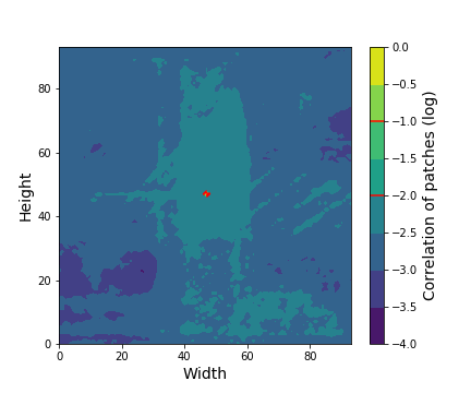
In this section we show that the quantity $q$ defined in Eq. 53, which computes the total correlation between degraded and clean patches, is much smaller than $|P|$. If this is the case, we know that the generalization bound given by Theorem 3.1 decreases with the number of patches $m$ and not with the number of images $n$, which confirms the fact that working at the patch level considerably reduced the amount of required training data.

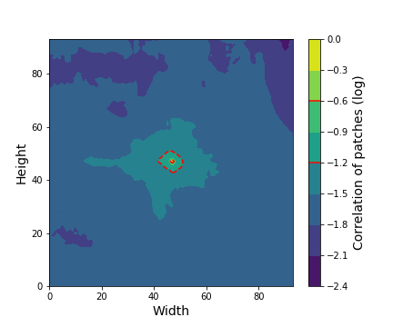
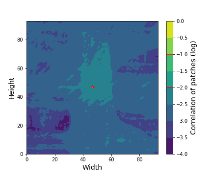
To empirically validate it, we show that the correlation of a patch (measured with the kernel used in our experiments described in Section 5), which uses DCT features, is high with patches of its neighborhood and small with patches far away. Looking at Eq. 53, this implies that the constant $q$ is independent of the total number of patches $|P|$.

We generate $n=250$ blurry images of size $101\times 101$ with the dataset of [29]. For each image, we compute the correlation of the central patch with the other patches. We decompose the images of the toy dataset into $8\times 8$ patches, leading to $|P|=8836$ patches per image. Figure 3 illustrates the average correlation coefficients for the central patch of the images for the 3 first iterations of HQS. At the first iteration, the correlations are computed on the blurry image and the subsequent iterations on the current estimates of the sharp image. One can notice a decay of the correlation coefficients below $1\%$ of the central correlation when we are outside a $5\times 5$ window around the central patch for iterations 2 and 3. For the first iteration, the decay is slower but patches outside a $5\times 5$ window around the central patch have a correlation below $6\%$. This validates the between locality assumption of Section 3.

Iteration 1.

Iteration 2.

Iteration 3.

Figure 3: Correlation of the central patch of the image with the rest of patches. We use DCT features and a Gaussian kernel with the same bandwidth than in our experiments.

C.2 Implementation Details

In this section, we present more details on the setting used to run the experiments and give a canvas of our Python implementation of SDCA with gap sampling.

C.2.1 Code of SDCA with gap sampling

We present here a simplified code canvas in Python for implementing Algorithm 1 with gap sampling, for clarity’s sake. We choose to use Pytorch to easily run the code on a GPU.

The variable “xtr” stands for the training images $\text{x}^{(i)}$ ($i=1,\dots,m$). The variable “gaps” is a $m\times|P|$ matrix that contains the dual gap for each pair of training sample $\text{x}^{(i)}$ and test patch $x_{p}$. Summing over the first axis yields the $|P|$ dual gaps for performing gap sampling.

⬇

1import torch

2

3def compute_dual_gaps(z, x, mu, alpha, xtr, beta):

4 # mu: shape (m,P,ps,ps)

5 # alpha: shape (m,P,1,1)

6 alpha = alpha.squeeze(-1).squeeze(-1)

7 z = z.unsqueeze(0)

8 x = x.unsqueeze(0)

9 xtr = xtr.unsqueeze(1)

10 g = alpha*(z - xtr).norm(p=2, dim=(-1,-2))

11 g += torch.einsum("ijkl,ijkl->ij", [mu, z-xtr])

12 return g

13

14def SDCA(x, alpha, xtr, beta, K, epsilon=1e-5):

15 # x: shape (P, ps, ps): initial guess

16 # alpha: shape (m, P, 1, 1)

17 # xtr: (m, ps, ps)

18 ## create the variables

19 n, P = alpha.shape[:2]

20 ps = xtr.shape[-1]

21 z = x

22 mu = torch.zeros(m, P, ps, ps)

23 ## compute first dual gaps

24 gaps = compute_dual_gaps(z, x, mu, alpha, xtr, beta)

25 ## do loop

26 k = 0

27 while gaps.sum(0).max() > epsilon and k < K:

28 _, i = gaps.max(dim=0) # gap sampling

29 b = z - mu[i] / beta - xtr[i]

30 nb = b.norm(p=2, dim=(-1,-2), keepdim=True)

31 mu_i = -b * torch.min(alpha[i] / nb, beta)

32 z += (mu_i - mu[i]) / beta

33 mu[i] = mu_i

34 # update all the gaps

35 gaps = compute_dual_gaps(z, x, mu, alpha, xtr, beta)

36 k += 1

37 return z

Listing 1: Python template for SDCA with gap sampling (Algorithm 1).

C.2.2 Additional details

We run the code on a NVIDIA V100 GPU with 32Gb of graphic memory.

One crucial element of our implementation is the design of the bandwidth $\sigma_{k}$ of the Gaussian kernel $k$. We compute the DCT features for the training patches $\text{x}^{(i)}$ ($i=1,\dots,m$), resulting in a $m\times d$ matrix (for $8\times 8$ patches, $d=64$). We then compute the standard deviations $\sigma^{1},\dots,\sigma^{d}$, one for each row of the feature matrix. Finally, we choose the bandwidth as $\sigma_{k}=s\|(\sigma^{1},\dots,\sigma^{d})\|_{2}$ with $s$ a scalar set to 0.2 in our implementation.

In practice, recomputing the dual gaps at each SDCA iterations is time-consuming. Instead, we update the dual gaps every 25 SDCA steps to reduce the computation time of the update of $z$. We have not noticed a drop of performance by doing so, compared to recomputing the dual gap at each iteration.

For deblurring, we run $T=8$ iterations of HQS in 6 minutes for a $321\times 481$ image of BSD68 [29] with $m=10000$ training samples. It could be greatly reduced by selecting a smaller set of training samples, i.e., selecting a smaller $m$, and is one of our lines of research. As a comparison, EPLL runs $T=6$ steps of HQS in about 3 minutes on our workstation for the same images.

C.3 Further Experiments

In this section, we present an ablation study we have run to select images to collect training patches from and our current results and observations for denoising.

C.3.1 Choice of datasets.

We first evaluate the impact of the diversity of the images used to build our training set of patches. We select 5 images depicting penguins, tigers, bears and buildings from the training set of BSD300 [29], select one from each class as test image and use the four others as training images to sample $m$ training pairs $(\text{x}^{(i)},\text{y}^{(i)})$. The images are blurred with kernel 2 from [23] and have $1\%$ additive Gaussian noise. In Table 3, the rows correspond to the test images to be deblurred an the columns are the compositions of the datasets. We use the same experimental setting than in the main paper for deblurring. “Penguin”, “Tiger”, “Bear” and “Building” correspond to sets of 4 images of the same class and “Hybrid” is a set made of one image of each class.

Table 3: Deblurring performance depending of the composition of the training set.

Tr. classes	Penguin	Tiger	Bear	Building	Hybrid
Penguin	29.64	29.51	29.31	28.68	29.69
Tiger	26.91	26.90	26.81	26.74	26.89
Bear	30.92	30.81	30.61	29.59	30.94
Building	24.44	24.49	24.46	24.81	24.49
Average	27.98	27.93	27.80	27.46	28.00

In Table 3, we show that when restoring an image with patches taken from images of the class, deblurring results are better. If now one restores a picture of an animal with images of another animal, performance are in the same ballpark, validating the fact that useful patches can be found in other images than the ones of the same class. Now if one takes images of buildings to restore images of animals, the performance drops on the images of the penguin and the bear by -1dB. A similar effect exists if one wants to restore an image of a building with images of animals where a drop of -0.4dB can be observed on the PSNR score the test image depicting a building.

This can be understood by the fact that images of buildings contain regular structures such as lines whereas images of animals feature landscapes and highly-textured surfaces such as furs and grass. Restraining the training patches to the sole building structures is less effective to restore these details.

Considering three images of animals and one image of a building leads to marginally better results in average than using specific classes for training. One can see that using only building images leads to a drop of -0.5dB in average compared to the other configurations, showing that variety of the training patches can have an important impact on the restoration performance.

Blurry image (21.51dB).

EPLL (31.93dB).

Ours ($\ell_{2}$, 30.11dB).

Ground-truth image.

Figure 4: A denoising example from Set12 [51], with $\sigma=15$, better seen on a computer screen. Even though our methods removes most of the noise and produces a decent result, it oversmooths textures and keep residual noise at the salient edges of the image such as the hands of the man whereas EPLL filters out the noise and conserves the high-frequency details, explaining the gap of nearly 2dB with our restored image.

C.3.2 Denoising

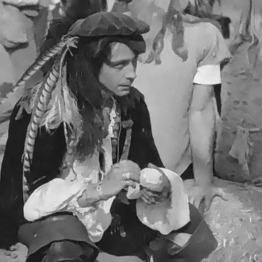
We use the classical dataset of 12 images used in [51] for denoising evaluation. We add Gaussian noise of standard deviation 15, 25 and 50 (for pixel values in [0,255]). We show comparisons with a sparse coding technique [15], a non-local means approach [13] and a GMM-based prior [52] in Table 4. We set $T=5$, $\delta=2$, $\beta_{0}=0.015$ and $\gamma=64,32$ and 16 for $\sigma=15,25$ and 50.

Table 4: Average PSNR for denoising.

Methods	KSVD [15]	BM3D [13]	EPLL [52]	Ours ($\ell_{2}$)
$\sigma=15$	31.98	32.36	32.10	29.39
$\sigma=25$	29.33	29.91	29.62	27.31
$\sigma=50$	24.82	26.20	26.32	24.44

We are clearly below standard variational methods for the task of denoising by margins of about -2dB to -3db for each considered noise level in terms of PSNR. This might be explained by the fact that denoising is a less structured problem than deblurring or upsampling, i.e., no information can be exploited from a forward operator $B$ that is in this case the identity. Thus, one must carefully design the coefficients $\alpha$ to filter out some noise during reconstruction. The DCT features appear to not be robust enough to noise and we will explore different features to circumvent this issue and improve the denoising performance of the proposed framework. A denoising example is given in Figure 4 where one can observe that most of the noise is removed and artifacts appear at the edges of the elements of the image such as the fingers of the man.

Appendix D Additional Images

In this section, we present additional images for non-blind deblurring and upsampling. The images are better seen on a computer screen. The metric is the PSNR.

D.1 Non-blind deblurring

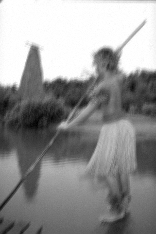
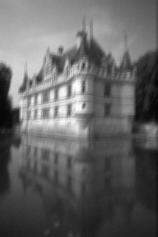
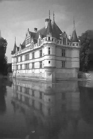
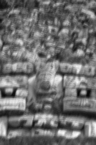
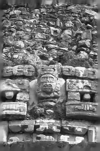
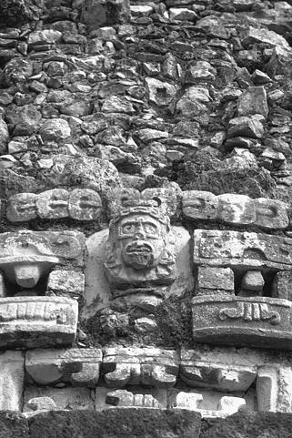
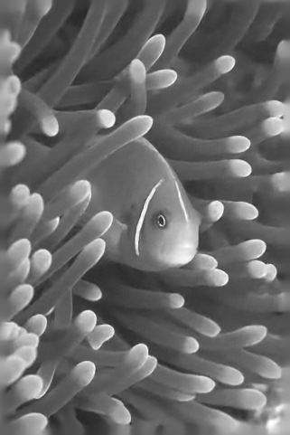
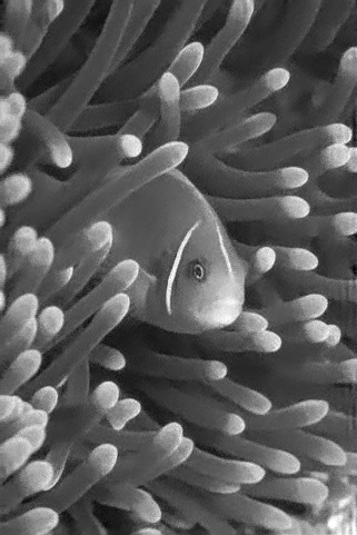
In this section we present more non-blind deblurring examples comparing EPLL and the $\ell_{2}$ version of the proposed framework on the test set of BSD [29] with the same experimental setting than presented in the main paper. The results are shown in Figures 5, 6, 7, 8 and 9. This demonstrates the practical ability of structured prediction to handle this task as well as a standard variational framework, i.e., EPLL [52], with a prior learned over 200000 patches.

Blurry image (24.28dB).

EPLL (28.10dB).

Ours ($\ell_{2}$, 29.60dB).

Ground-truth image.

Figure 5: A non-blind deblurring example from BSD68 [29].

Blurry image (24.37dB).

EPLL (29.84dB).

Ours ($\ell_{2}$, 28.89dB).

Ground-truth image.

Figure 6: A non-blind deblurring example from BSD68 [29].

Blurry image (21.51dB).

EPLL (22.76dB).

Ours ($\ell_{2}$, 23.65dB).

Ground-truth image.

Figure 7: A non-blind deblurring example from BSD68 [29].

Blurry image (24.07dB).

EPLL (29.49dB).

Ours ($\ell_{2}$, 31.71dB).

Ground-truth image.

Figure 8: A non-blind deblurring example from BSD68 [29].

Blurry image (24.60dB).

EPLL (29.20dB).

Ours ($\ell_{2}$, 28.77dB).

Ground-truth image.

Figure 9: A non-blind deblurring example from BSD68 [29].

D.2 Upsampling

In this section, we present qualitative results for upsampling by a factor $\times 2$ by comparing the $\ell_{2}$ version of our method with an image obtained by bicubic interpolation, KSVD [49], GR and ANR, two variants of [43]. The images are taken from the Set5 dataset [43] and we followed the same experimental protocol than in the paper. The results are shown in Figures 10, 11 and 12. For each image we do better than bicubic interpolation but fail behind ANR and KSVD. The differences explaining are results below other standard dictionary learning methdods are aliasing artifacts on the beak of the bird in Figure 10, the black edges on the wings of the butterfly Figure 11 and the fingeres and sleeves of the woman Figure 12. These details are better seen on a computer screen.

Bicubic (36.8dB).

KSVD (39.9dB).

GR (39.0dB).

ANR (40.0dB).

Ours ($\ell_{2}$, 38.9dB).

Ground-truth image.

Figure 10: An upsampling example from Set5 [43].

Bicubic (27.4dB).

KSVD (30.6dB).

GR (29.1dB).

ANR (30.5dB).

Ours ($\ell_{2}$, 30.0dB).

Ground-truth image.

Figure 11: An upsampling example from Set5 [43].

Bicubic (32.1dB).

KSVD (34.5dB).

GR (33.7dB).

ANR (34.5dB).

Ours ($\ell_{2}$, 34.0dB).

Ground-truth image.

Figure 12: An upsampling example from Set5 [43].

References

- [1] A. Abdelhamed, S. Lin, and M. S. Brown. A high-quality denoising dataset for smartphone cameras. In Proceedings of the conference on Computer Vision and Pattern Recognition, pages 1692–1700, 2018.
- [2] R. A. Adams and J. J. Fournier. Sobolev spaces. Elsevier, 2003.
- [3] N. Aronszajn. Theory of reproducing kernels. Transactions of the American mathematical society, 68(3):337–404, 1950.
- [4] A. Berlinet and C. Thomas-Agnan. Reproducing kernel Hilbert spaces in probability and statistics. Springer Science & Business Media, 2011.
- [5] A. Buades, B. Coll, and J. Morel. A non-local algorithm for image denoising. In Proceedings of the conference on Computer Vision and Pattern Recognition, pages 60–65, 2005.
- [6] A. Caponnetto and E. De Vito. Optimal rates for the regularized least-squares algorithm. Foundations of Computational Mathematics, 7(3):331–368, 2007.
- [7] P. Chatterjee and P. Milanfar. Patch-based near-optimal image denoising. IEEE Transactions on Image Processing, 21(4):1635–1649, 2012.
- [8] Y. Chen and T. Pock. Trainable nonlinear reaction diffusion: A flexible framework for fast and effective image restoration. IEEE Transactions on Pattern Analysis and Machine Intelligence, 39(6):1256–1272, 2017.
- [9] C. Ciliberto, F. Bach, and A. Rudi. Localized structured prediction. In Advances on Neural Information Processing Systems, pages 7299–7309, 2019.
- [10] C. Ciliberto, L. Rosasco, and A. Rudi. A consistent regularization approach for structured prediction. In Advances on Neural Information Processing Systems, pages 4412–4420, 2016.
- [11] C. Ciliberto, L. Rosasco, and A. Rudi. A general framework for consistent structured prediction with implicit loss embeddings. Journal of Machine Learning Research, page to appear, 2020.
- [12] C. Ciliberto, A. Rudi, L. Rosasco, and M. Pontil. Consistent multitask learning with nonlinear output relations. In Advances on Neural Information Processing Systems, pages 1986–1996, 2017.
- [13] K. Dabov, A. Foi, V. Katkovnik, and K. O. Egiazarian. Image denoising by sparse 3-D transform-domain collaborative filtering. IEEE Transactions on Image Processing, 16(8):2080–2095, 2007.
- [14] C. Dong, C. C. Loy, K. He, and X. Tang. Image super-resolution using deep convolutional networks. IEEE Transactions on Pattern Analysis and Machine Intelligence, 38(2):295–307, 2016.
- [15] M. Elad and M. Aharon. Image denoising via sparse and redundant representations over learned dictionaries. IEEE Transactions on Image Processing, 15(12):3736–3745, 2006.
- [16] S. Farsiu, M. D. Robinson, M. Elad, and P. Milanfar. Advances and challenges in super-resolution. International Journal on Imaging Systems and Technology, 14(2):47–57, 2004.
- [17] W. T. Freeman, T. R. Jones, and E. C. Pasztor. Example-based super-resolution. IEEE Computer Graphics and Applications, 22(2):56–65, 2002.
- [18] D. Geman and C. Yang. Nonlinear image recovery with half-quadratic regularization. IEEE Transactions on Image Processing, 5(7):932–946, 1995.
- [19] D. Glasner, S. Bagon, and M. Irani. Super-resolution from a single image. In Proceedings of the International Conference on Computer Vision, pages 349–356, 2009.
- [20] K. He and J. Sun. Image completion approaches using the statistics of similar patches. IEEE Transactions on Pattern Analysis and Machine Intelligence, 36(12):2423–2435, 2014.
- [21] L. Jacob, G. Obozinski, and J. Vert. Group lasso with overlap and graph lasso. In Proceedings of the International Conference on Machine Learning, pages 433–440, 2009.
- [22] V. Katkovnik, A. Foi, K. O. Egiazarian, and J. Astola. From local kernel to nonlocal multiple-model image denoising. International Journal on Computer Vision, 86(1):1–32, 2010.
- [23] D. Krishnan and R. Fergus. Fast image deconvolution using hyper-Laplacian priors. In Advances on Neural Information Processing Systems, pages 1033–1041, 2009.
- [24] R. Le Priol, A. Piché, and S. Lacoste-Julien. Adaptive stochastic dual coordinate ascent for conditional random fields. In Proceedings of the Conference on Uncertainty in Artificial Intelligence (UAI), pages 815–824, 2018.
- [25] J. Mairal, F. Bach, and J. Ponce. Sparse modeling for image and vision processing. Foundations and Trends® in Computer Graphics and Vision, 8(2-3):85–283, 2014.
- [26] J. Mairal, F. Bach, J. Ponce, and G. Sapiro. Online learning for matrix factorization and sparse coding. Journal of Machine Learning Research, 11:19–60, 2010.
- [27] J. Mairal, F. Bach, J. Ponce, G. Sapiro, and A. Zisserman. Non-local sparse models for image restoration. In Proceedings of the International Conference on Computer Vision, pages 2272–2279, 2009.
- [28] U. Marteau-Ferey, F. Bach, and A. Rudi. Globally convergent newton methods for ill-conditioned generalized self-concordant losses. In Advances in Neural Information Processing Systems, pages 7634–7644, 2019.
- [29] D. R. Martin, C. C. Fowlkes, D. Tal, and J. Malik. A database of human segmented natural images and its application to evaluating segmentation algorithms and measuring ecological statistics. In Proceedings of the International Conference on Computer Vision, pages 416–425, 2001.
- [30] E. A. Nadaraya. On estimating regression. Teor. Veroyatnost. i Primenen., 9(1):157–159, 1964.
- [31] A. Osokin, J. Alayrac, I. Lukasewitz, P. K. Dokania, and S. Lacoste-Julien. Minding the gaps for block frank-wolfe optimization of structured svms. In Proceedings of the International Conference on Machine Learning (ICML), pages 593–602, 2016.
- [32] N. Parikh and S. P. Boyd. Proximal algorithms. Foundations and Trends in Optimization, 1(3):127–239, 2014.
- [33] E. Parzen. On estimation of a probability density function and mode. The annals of mathematical statistics, 33(3):1065–1076, 1962.
- [34] R. T. Rockafellar. Convex analysis. Number 28. Princeton university press, 1970.
- [35] L. I. Rudin, S. Osher, and E. Fatemi. Nonlinear total variation based noise removal algorithms. Physica D, 60:259–268, 1992.
- [36] B. Schölkopf, A. J. Smola, F. Bach, et al. Learning with kernels: support vector machines, regularization, optimization, and beyond. MIT press, 2002.
- [37] S. Shalev-Shwartz. SDCA without duality, regularization, and individual convexity. In Proceedings of the International Conference on Machine Learning, pages 747–754, 2016.
- [38] S. Shalev-Shwartz. Sdca without duality, regularization, and individual convexity. In International Conference on Machine Learning, pages 747–754, 2016.
- [39] S. Shalev-Shwartz and T. Zhang. Stochastic dual coordinate ascent methods for regularized loss minimization. Journal of Machine Learning Research, 14(Feb):567–599, 2013.
- [40] J. Starck and F. Murtagh. Astronomical Image and Data Analysis, Second Edition. Astronomy and Astrophysics Library. Springer, 2006.
- [41] J. Sun, J. Zhu, and M. F. Tappen. Context-constrained hallucination for image super-resolution. In Proceedings of the conference on Computer Vision and Pattern Recognition, pages 231–238, 2010.
- [42] H. Takeda, S. Farsiu, and P. Milanfar. Kernel regression for image processing and reconstruction. IEEE Transactions on Image Processing, 16(2):349–366, 2007.
- [43] R. Timofte, V. D. Smet, and L. V. Gool. Anchored neighborhood regression for fast example-based super-resolution. In Proceedings of the International Conference on Computer Vision, pages 1920–1927, 2013.
- [44] V. Vapnik. The nature of statistical learning theory. Springer science & business media, 2013.
- [45] R. Vershynin. High-dimensional probability: An introduction with applications in data science, volume 47. Cambridge university press, 2018.
- [46] Y. Wang, J. Yang, W. Yin, and Y. Zhang. A new alternating minimization algorithm for total variation image reconstruction. SIAM Journal on Imaging Sciences, 1(3):248–272, 2008.
- [47] M. Weigert, U. Schmidt, T. Boothe, A. Müller, A. Dibrov, A. Jain, B. Wilhelm, D. Schmidt, C. Broaddus, S. Culley, M. Rocha-Martins, F. Segovia-Miranda, C. Norden, R. Henriques, M. Zerial, M. Solimena, J. Rink, P. Tomancak, L. Royer, F. Jug, and E. W. Myers. Content-aware image restoration: Pushing the limits of fluorescence microscopy. Nature Methods, 15(12):1090–1097, 2018.
- [48] N. Wiener. Extrapolation, Interpolation, and Smoothing of Stationary Time Series. Wiley, 1949.
- [49] R. Zeyde, M. Elad, and M. Protter. On single image scale-up using sparse-representations. In Proceedings of the International Conference on Curves and Surfaces, pages 711–730, 2010.
- [50] J. Zhang, J. Pan, W. Lai, R. W. H. Lau, and M. Yang. Learning fully convolutional networks for iterative non-blind deconvolution. In Proceedings of the conference on Computer Vision and Pattern Recognition, pages 6969–6977, 2017.
- [51] K. Zhang, W. Zuo, Y. Chen, D. Meng, and L. Zhang. Beyond a gaussian denoiser: Residual learning of deep CNN for image denoising. IEEE Transactions on Image Processessing, 26(7):3142–3155, 2017.
- [52] D. Zoran and Y. Weiss. From learning models of natural image patches to whole image restoration. In Proceedings of the International Conference on Computer Vision, pages 479–486, 2011.