Abstract

We study the problem of corralling stochastic bandit algorithms, that is combining multiple bandit algorithms designed for a stochastic environment, with the goal of devising a corralling algorithm that performs almost as well as the best base algorithm. We give two general algorithms for this setting, which we show benefit from favorable regret guarantees. We show that the regret of the corralling algorithms is no worse than that of the best algorithm containing the arm with the highest reward, and depends on the gap between the highest reward and other rewards.

1 Introduction

We study the problem of corralling multi-armed bandit algorithms in a stochastic environment. This consists of selecting, at each round, one out of a fixed collection of bandit algorithms and playing the action returned by that algorithm. Note that the corralling algorithm does not directly select an arm, but only a base algorithm. It never requires knowledge of the action set of each base algorithm. The objective of the corralling algorithm is to achieve a large cumulative reward or a small pseudo-regret, over the course of its interactions with the environment. This problem was first introduced and studied by Agarwal et al. (2016). Here, we are guided by the same motivation but consider the stochastic setting and seek more favorable guarantees. Thus, we assume that the reward, for each arm, is drawn from an unknown distribution.

In the simplest setting of our study, we assume that each base bandit algorithm has access to a distinct set of arms. This scenario appears in several applications. As an example, consider the online contractual display ads allocation problem (BasuMallick, 2020): when users visit a website, say some page of the online site of a national newspaper, an ads allocation algorithm chooses an ad to display at each specific slot with the goal of achieving the largest value. This could be an ad for a clothing item, which could be meant for the banner of the online front page of that newspaper. To do so, the ads allocation algorithm chooses one out of a large set of advertisers, each a clothing brand or company in this case, which have signed a contract with the ads allocation company. Each clothing company has its own marketing strategy and thus its own bandit algorithm with its own separate set of clothing items or arms. There is no sharing of information between these companies which are typically competitors. Furthermore, the ads allocation algorithm is not provided with any detailed information about the base bandits algorithms of these companies, since that is proprietary information private to each company. The allocation algorithm cannot choose a specific arm or clothing item, it can only choose a base advertiser. The number of ads or arms can be very large. The number of advertisers can also be relatively large in practice, depending on the domain. The number of times the ads allocation is run is in the order of millions or even billions per day, depending on the category of items.

A similar problem arises with online mortgage broker companies offering loans to new applicants. The mortgage broker algorithm must choose a bank, each with different mortgage products. The broker brings a new application exclusively to one of the banks, as part of the contract, which also entitles them to incentives. The bank’s online algorithm can be a bandit algorithm proposing a product, and the details of the algorithm are not accessible to the broker; for instance, the bank’s credit rate and incentives may depend on the financial and credit history of the applicant. The number of mortgage products is typically fairly large, and the number of online loan requests per day is in the order of several thousands. Other instances of this problem appear when an algorithm can only select one of multiple bandit algorithms and, for privacy or regulatory reasons, it cannot directly select an arm or receive detailed information about the base algorithms.

In the most general setting we study, there may be an arbitrary sharing of arms between the bandit algorithms. We will only assume that only one algorithm has

access to the arm with maximal expected reward, which implies a positive gap between the expected reward of the best arm of any algorithm and that of the best algorithm. This is because we seek to devise a corralling algorithm with favorable gap-dependent pseudo-regret guarantees.

Related work. The previous work most closely related to this study is the seminal contribution by Agarwal et al. (2016) who initiated the general problem of corralling bandit algorithms. The authors gave a general algorithm for this problem, which is an instance of the generic Mirror Descent algorithm with an appropriate mirror map (Log-Barrier-OMD), (Foster et al., 2016; Wei and Luo, 2018), and which includes a carefully constructed non-decreasing step-size schedule, also used by Bubeck et al. (2017). The algorithm of Agarwal et al. (2016), however, cannot in general achieve regret bounds better than $\tilde{O}(\sqrt{T})$ in the time horizon, unless optimistic instance-dependent regret bounds are known for the corralled algorithms. Prior to their work, Arora et al. (2012) presented an algorithm for learning deterministic Markov decision processes (MDPs) with adversarial rewards, using an algorithm for corralling bandit linear optimization algorithms. In an even earlier work, Maillard and Munos (2011) attempted to corral EXP3 algorithms (Auer et al., 2002b) with a top algorithm that is a slightly modified version of EXP4. The resulting regret bounds are in $\tilde{O}(T^{2/3})$.

Our work can also be viewed as selecting the best algorithm for a given unknown environment and, in this way, is similar in spirit to the literature solving the best of both worlds problem (Audibert and Bubeck, 2009; Bubeck and Slivkins, 2012; Seldin and Slivkins, 2014; Auer and Chiang, 2016; Seldin and Lugosi, 2017; Wei and Luo, 2018; Zimmert and Seldin, 2018; Zimmert et al., 2019) and the model selection problem for linear bandit (Foster et al., 2019; Chatterji et al., 2019).

Very recently, Pacchiano et al. (2020) also considered the problem of corralling stochastic bandit algorithms. The authors seek to treat the problem of model selection, where multiple algorithms might share the best arm. More precisely, the authors consider a setting in which there are $K$ stochastic contextual bandit algorithms and try to minimize the regret with respect to the best overall policy belonging to any of the bandit algorithms. They propose two corralling algorithms, one based on the work of (Agarwal et al., 2016) and one based on EXP3.P (Auer et al., 2002b). The main novelty in their work is a smoothing technique for each of the base algorithms, which avoids having to restart the base algorithms throughout the $T$ rounds, as was proposed in (Agarwal et al., 2016). The proposed regret bounds are of the order $\tilde{\Theta}(\sqrt{T})$. We expect that the smoothing technique is also applicable to one of the corralling algorithms we propose. Since Pacchiano et al. (2020) allow for algorithms with shared best arms, their main results do not discuss the optimistic setting in which there is a gap between the reward of the optimal policy and all other competing policies, and do not achieve the optimistic guarantees we provide. Further, they show a min-max lower bound which states that even if one of the base algorithms is optimistic and contains the best arm, there is still no hope to achieve regret better than $\tilde{\Omega}(\sqrt{T})$ if the best arm is shared by an algorithm with regret $\tilde{\Omega}(\sqrt{T})$. We view their contributions as complementary to ours.

In general, some caution is needed when designing a corralling algorithm, since aggressive strategies may discard or disregard a base learner that admits an arm with the best mean reward if it performs poorly in the initial rounds. Furthermore, as noted by Agarwal et al. (2016), additional assumptions are required on each of the base learners if one hopes to achieve non-trivial corralling guarantees.

Contributions. We first motivate our key assumption that all of the corralled algorithms must have favorable regret guarantees during all rounds. To do so, in Section 3, we show that if one does not assume anytime regret guarantees, then even when corralling simple stochastic bandit algorithms, each with $o(\sqrt{T})$ regret, any corralling strategy will have to incur $\Omega(\sqrt{T})$ regret. Therefore, for the rest of the paper we assume that each base learner admits anytime guarantees. In Section 4 and Section 5, we present two general corralling algorithms whose pseudo-regret guarantees admit a dependency on the gaps between base learners, that is their best arms, and only poly-logarithmic dependence on time horizon. These bounds are syntactically similar to the instance-dependent guarantees for the stochastic multi-armed bandit problem (Auer et al., 2002a). Thus, our corralling algorithm performs almost as well as the best base learner, if it were to be used on its own, modulo gap-dependent terms and logarithmic factors. The algorithm in Section 4 uses the standard UCB ideas combined with a boosting technique, which runs multiple copies of the same base learner. In Section 4.1, we show that simply using UCB-style corralling without boosting can incur linear regret. If, additionally, we assume that each of the base learners satisfy the stability condition adopted in (Agarwal et al., 2016), then, in Section 5 we show that it suffices to run a single copy of each base learner by using a corralling approach based on OMD. We show that UCB-I (Auer et al., 2002a) can be made to satisfy the stability condition, as long as the confidence bound is rescaled and changed by an additive factor. In Section 6, to further examine the properties of our algorithms, we report the results of experiments with our algorithms for synthetic datasets. Finally, while our main motivation is not model selection, in Section 7, we briefly discuss some related matters and show that our algorithms can help recover several known results in that area.

2 Preliminaries

We consider the problem of corralling $K$ stochastic multi-armed bandit algorithms $\mathcal{A}_{1},\ldots,\mathcal{A}_{K}$, which we often refer to as base algorithms (base learners). At each round $t$, a corralling algorithm selects a base algorithm $\mathcal{A}_{i_{t}}$, which plays action $a_{i_{t},j_{t}}$. The corralling algorithm is not informed of the identity of this action but it does observe its reward $r_{t}(a_{i_{t},j_{t}})$. The top algorithm then updates its decision rule and provides feedback to each of the base learners $\mathcal{A}_{i}$. We note that the feedback may be just the empty set, in which case the base learners do not update their state. We will also assume access to the parameters controlling the behavior of each $\mathcal{A}_{i}$ such as the step size for mirror descent-type algorithms, or the confidence bounds for UCB-type algorithms. Our goal is to minimize the cumulative pseudo-regret of the corralling algorithm as defined in Equation 1:

$$\mathbb{E}[R(T)]=T\mu_{1,1}-\mathbb{E}\left[\sum_{t=1}^{T}r_{t}(a_{i_{t},j_{t}})\right],$$ (1)

where $\mu_{1,1}$ is the mean reward of the best arm.

Notation. We denote by $\mathrm{e}_{i}$ the $i$th standard basis vector, by $\boldsymbol{0}_{K}\in\mathbb{R}^{K}$ the vector of all $0$s, and by $\boldsymbol{1}_{K}\in\mathbb{R}^{K}$ the vector of all $1$s. For two vectors $x,y\in\mathbb{R}^{K}$, $x\odot y$ denotes their Hadamard product. We also denote the line segment between $x$ and $y$ as $[x,y]$. $w_{t,i}$ denotes the $i$-th entry of a vector $w_{t}\in\mathbb{R}^{K}$. $\Delta^{K-1}$ denotes the probability simplex in $\mathbb{R}^{K}$, $D_{\Psi}(x,y)$ the Bregman divergence induced by the potential $\Psi$, whose conjugate function we denote by $\Psi^{*}$. We use $\mathrm{I}_{C}$ to denote the indicator function of a set $C$. For any $k\in\mathbb{N}$, we use the shorthand $[k]:=\{1,2,\ldots,k\}$.

For the base algorithms $\mathcal{A}_{1},\ldots,\mathcal{A}_{K}$, let $T_{i}(t)$ be the number of times algorithm $\mathcal{A}_{i}$ has been played until time $t$. Let $T_{i,j}(t)$ be the number of times action $j$ has been proposed by algorithm $\mathcal{A}_{i}$ until time $t$. Let $[k_{i}]$ denote the set of arms or action set of algorithm $\mathcal{A}_{i}$. We denote the reward of arm $j$ in the action set of algorithm $i$ at time $t$ as $r_{t}(a_{i,j})$ and denote its mean reward by $\mu_{i,j}$. We also use $a_{i,j_{t}}$ to denote the arm proposed by algorithm $\mathcal{A}_{i}$ during time $t$. Further, the algorithm played at time $t$ is denoted as $i_{t}$, its action played at time $t$ is $a_{i_{t},j_{t}}$ and the reward for that action is $r_{t}(a_{i_{t},j_{t}})$ with mean $\mu_{i_{t},j_{t}}$. Let $i^{*}$ denote the index of the base algorithm that contains the arm with the highest mean reward. Without loss of generality, we will assume that $i^{*}=1$. Similarly, we assume that $a_{i,1}$ is the arm with highest reward in algorithm $\mathcal{A}_{i}$. We assume that the best arm of the best algorithm has a gap to the best arm of every other algorithm. We denote the gap between the best arm of $\mathcal{A}_{1}$ and the best arm of $\mathcal{A}_{i}$ as $\Delta_{i}$: $\Delta_{i}=\mu_{i^{*},1}-\mu_{i,1}>0$ for $i\neq i^{*}$. Further, we denote the intra-algorithm gaps by $\Delta_{i,j}=\mu_{i,1}-\mu_{i,j}$. We denote by $\bar{R}_{i}(t)$ an upper bound on the regret of algorithm $\mathcal{A}_{i}$ at time $t$ and by $R_{i}(t)$ the actual regret of $\mathcal{A}_{i}$, so that $\mathbb{E}[R_{i}(t)]$ is the expected regret of algorithm $\mathcal{A}_{i}$ at time $t$. The asymptotic notations $\tilde{\Omega}$ and $\tilde{O}$ are equal to $\Omega$ and $O$ up to poly-logarithmic factors.

3 Lower bounds without anytime regret guarantees

We begin by showing a simple and yet instructive lower bound that helps guide our intuition regarding the information needed from the base algorithms $\{\mathcal{A}_{i}\}_{i=1}^{K}$ in the design of a corralling algorithm. Our lower bound is based on corralling base algorithms that only admit a fixed-time horizon regret bound and do not enjoy anytime regret guarantees. We further assume that the corralling strategy cannot simulate anytime regret guarantees on the base algorithms, say by using the so-called doubling trick. This result suggests that the base algorithms must admit a strong regret guarantee during every round of the game.

The key idea behind our construction is the following. Suppose one of the corralled algorithms, $\mathcal{A}_{i}$, incurs a linear regret over the first $R_{i}(T)$ rounds. In that case, the corralling algorithm is unable to distinguish between $\mathcal{A}_{i}$ and an another algorithm that mimics the linear regret behavior of $\mathcal{A}_{i}$ throughout all $T$ rounds, unless the corralling algorithm plays $\mathcal{A}_{i}$ at least $R_{i}(T)$ times. The successive elimination algorithm (Even-Dar et al., 2002) benefits from gap-dependent bounds and can have the behavior just described for a base algorithm. Thus, our lower bound is presented for successive elimination base algorithms, all with regret $O(T^{1/4})$. It shows that, with constant probability, no corralling strategy can achieve a more favorable regret than $\tilde{\Omega}(\sqrt{T})$ in that case.

Theorem 3.1.

Let the corralled algorithms be instances of successive elimination defined by a parameter $\alpha$. With probability $1/4$ over the random sampling of $\alpha$, any corralling strategy will incur regret at least $\tilde{\Omega}(\sqrt{T})$, while the gap, $\Delta$, between the best and second best reward is such that $\Delta>\omega(T^{-1/4})$ and all algorithms have a regret bound of $\tilde{O}(1/\Delta)$.

This theorem shows that, even when corralling natural algorithms that benefit from asymptotically better regret bounds, corralling can incur $\tilde{\Omega}(\sqrt{T})$ regret. It can be further proven (Theorem B.3, Appendix B) that, even if the worst case upper bounds on the regret of the base algorithms were known, achieving an optimistic regret guarantee for corralling would not be possible, unless some additional assumptions were made.

4 UCB-style corralling algorithm

The negative result of Section 3 hinge on the fact that the base algorithms do not admit anytime regret guarantees. Therefore, we assume, for the rest of the paper, that the base algorithms, $\{\mathcal{A}_{i}\}$, satisfy the following:

$$\mathbb{E}\left[t\mu_{i,1}-\sum_{s=1}^{t}r_{s}(a_{i_{s},j_{s}})\right]\leq\bar{R}_{i}(t),$$ (2)

for any time $t\in[T]$. For UCB-type algorithms, such bounds can be derived from the fact that the expected number of pulls, $T_{i,j}(t)$, of a suboptimal arm $j$, is bounded as $\mathbb{E}[T_{i,j}(t)]\leq c\frac{\operatorname{log}\left(t\right)}{(\Delta_{i,j})^{2}}$, for some time and gap-independent constant $c$ (e.g., Bubeck (2010)), and take the following form, $\bar{R}_{i}(t)\leq c^{\prime}\sqrt{k_{i}t\operatorname{log}\left(t\right)}$, for some constant $c^{\prime}$.

Suppose that the bound in Equation 2 holds with probability $1-\delta_{t}$. Note that such bounds are available for some UCB-type algorithms (Audibert et al., 2009). We can then adopt the optimism in the face of uncertainty principle for each $\mu_{i,1}$ by overestimating it with $\frac{1}{t}\sum_{s=1}^{t}r_{s}(a_{i,j_{s}})+\frac{1}{t}\bar{R}_{i}(t)$. As long as this occurs with high enough probability, we can construct an upper confidence bound for $\mu_{i,1}$ and use it in a UCB-type algorithm. Unfortunately, the upper confidence bounds required for UCB-type algorithms to work need to hold with high enough probability, which is not readily available from Equation 2 or from probabilistic bounds on the pseudo-regret of anytime stochastic bandit algorithms. In fact, as discussed in Section 4.1, we expect it to be impossible to corral any-time stochastic MAB algorithms with a standard UCB-type strategy. However, a simple boosting technique, in which we run $2\operatorname{log}\left(1/\delta\right)$ copies of each algorithm $\mathcal{A}_{i}$, gives the following high probability version of the bound in Equation 2.

Lemma 4.1.

Suppose we run $2\operatorname{log}\left(1/\delta\right)$ copies of algorithm $\mathcal{A}_{i}$ which satisfies Equation 2. If $\mathcal{A}_{med_{i}}$ is the algorithm with median cumulative reward at time $t$, then $\mathbb{P}[t\mu_{i,1}-\sum_{s=1}^{t}r_{s}(a_{med_{i},j_{s}})\geq 2\bar{R}_{i}(t)]\leq\delta$.

Algorithm 1 UCB-C

0:  Stochastic bandit algorithms $\mathcal{A}_{1},\ldots,\mathcal{A}_{K}$

0:  Sequence of algorithms $(i_{t})_{t=1}^{T}$.

1:  $t=1$

2:  for $i=1,\ldots,K$ 

3:     $\mathbb{A}_{i}=\emptyset$ % contains all copies of $\mathcal{A}_{i}$

4:     for $s=1,\ldots,\lceil 2\operatorname{log}\left(T\right)\rceil$ 

5:        Initialize $\mathcal{A}_{i}(s)$ as a copy of $\mathcal{A}_{i}$, $\widehat{\mu}_{i}(s)=0$

6:        Append $(\mathcal{A}_{i}(s),\widehat{\mu}_{i}(s))$ to $\mathbb{A}_{i}$

7:  for $i=1,\ldots,K$ 

8:     Foreach $(\mathcal{A}_{i}(s),\widehat{\mu}_{i}(s))\in\mathbb{A}_{i}$, play $\mathcal{A}_{i}(s)$, update empirical mean $\widehat{\mu}_{i}(s)$, $t=t+2\operatorname{log}\left(T\right)$

9:     $\widehat{\mu}_{med_{i}}=\texttt{Median}(\{\widehat{\mu}_{i}(s)\}_{s=1}^{\lceil 2\operatorname{log}\left(T\right)\rceil})$

10:  while $t\leq T$ 

11:     $b_{\ell}(t)=\frac{\sqrt{2\bar{R}_{med_{\ell}}(T_{med_{\ell}}(t))}+\sqrt{2T_{med_{\ell}}(t)\operatorname{log}\left(t\right)}}{T_{med_{\ell}}(t)},\forall\ell\in[K]$

12:     $i=\operatorname*{\rm argmax}_{\ell\in[K]}\left\{\widehat{\mu}_{med_{\ell}}+b_{\ell}(t)\right\}$

13:     Foreach $(\mathcal{A}_{i}(s),\widehat{\mu}_{i}(s))\in\mathbb{A}_{i}$, play $\mathcal{A}_{i}(s)$, update empirical mean $\widehat{\mu}_{i}(s)$, $t=t+2\operatorname{log}\left(T\right)$

14:     $\widehat{\mu}_{med_{i}}=\texttt{Median}(\{\widehat{\mu}_{i}(s)\}_{s=1}^{\lceil 2\operatorname{log}\left(T\right)\rceil})$

We consider the following variant of the standard UCB algorithm for corralling. We initialize $2\operatorname{log}\left(T\right)$ copies of each base algorithm $\mathcal{A}_{i}$. Each $\mathcal{A}_{i}$ is associated with the median empirical average reward of its copies. At each round, the corralling algorithm picks the $\mathcal{A}_{i}$ with the highest sum of median empirical average reward and an upper confidence bound based on Lemma 4.1. The pseudocode is given in Algorithm 1. The algorithm admits the following regret guarantees.

Theorem 4.2.

Suppose that algorithms $\mathcal{A}_{1},\ldots,\mathcal{A}_{K}$ satisfy the following regret bound $\mathbb{E}[R_{i}(t)]\leq\sqrt{\alpha k_{i}t\operatorname{log}\left(t\right)}$, respectively for $i\in[K]$. Algorithm 1 selects a sequence of algorithms $i_{1},\ldots,i_{T}$ which take actions $a_{i_{1},j_{1}},\ldots,a_{i_{T},j_{T}}$, respectively, such that

$$\mathbb{E}[R(T)] \leq O\left(\sum_{i\neq i^{*}}\frac{k_{i}\operatorname{log}\left(T\right)^{2}}{\Delta_{i}}+\operatorname{log}\left(T\right)\mathbb{E}\left[R_{i^{*}}(T)\right]\right),$$

$$\mathbb{E}[R(T)] \leq O\left(\operatorname{log}\left(T\right)\sqrt{KT\operatorname{log}\left(T\right)\max_{i\in[K]}(k_{i})}\right).$$

We note that both the optimistic and the worst case regret bounds above involve an additional factor that depends on the number of arms, $k_{i}$, of the base algorithm $\mathcal{A}_{i}$. This dependence reflects the complexity of the decision space of algorithm $\mathcal{A}_{i}$. We conjecture that a complexity-free bound is not possible, in general. To see this, consider a setting where each $\mathcal{A}_{i}$, for $i\neq i^{*}$, only plays arms with equal means $\mu_{i}=\mu_{1,1}-\Delta_{i}$. Standard stochastic bandit regret lower bounds, e.g. (Garivier et al., 2018b), state that any strategy on the combined set of arms of all algorithms will incur regret at least $\Omega(\sum_{i\neq i^{*}}k_{i}\operatorname{log}\left(T\right)/\Delta_{i})$. The $\operatorname{log}\left(T\right)$ factor in front of the regret of the best algorithm comes from the fact that we are running $\Omega(\operatorname{log}\left(T\right))$ copies of it.

4.1 Discussion regarding tightness of bounds

A natural question is if it is possible to achieve bounds that do not have a $\operatorname{log}\left(T\right)^{2}$ scaling. After all, for the simpler stochastic MAB problem, regret upper bounds only scale as $O(\operatorname{log}\left(T\right))$ in terms of the time horizon. As already mentioned, the extra logarithmic factor comes from the boosting technique, or, more precisely, the need for exponentially fast concentration of the true regret to its expected value, when using a UCB-type corralling strategy. We now show that, in the absence of such strong concentration guarantees, if only a single copy of each of the base algorithms in Algorithm 1 is run, then linear regret is unavoidable.

Theorem 4.3.

There exist instances $\mathcal{A}_{1}$ and $\mathcal{A}_{2}$ of UCB-I and a reward distribution, such that, if Algorithm 1 runs a single copy of $\mathcal{A}_{1}$ and $\mathcal{A}_{2}$, then $\mathbb{E}[R(T)]\geq\tilde{\Omega}(\Delta_{2}T).$

Further, for any algorithm $\mathcal{A}_{1}$ such that $\mathbb{P}\left[R_{1}(t)\geq\frac{1}{2}\Delta_{1,2}\tau\right]\geq\frac{1}{\tau^{c}}$, there exists a reward distribution such that if Algorithm 1 runs a single copy of $\mathcal{A}_{1}$ and $\mathcal{A}_{2}$, then $\mathbb{E}[R(T)]\geq\tilde{\Omega}((\Delta_{1,2})^{c}\Delta_{2}T)$.

The proof of the above theorem and further discussion can be found in Appendix C.1. The requirement that the regret of the best algorithm satisfies $\mathbb{P}[R_{1}(t)\geq\frac{1}{2}\Delta_{1,2}\tau]\geq\frac{1}{\tau^{c}}$ in Theorem 4.3 is equivalent to the condition that the regret of the base algorithms admit only a polynomial concentration. Results in (Salomon and Audibert, 2011) suggest that there cannot be a tighter bound on the tail of the regret for anytime algorithms. It is therefore unclear if the $\operatorname{log}\left(T\right)^{2}$ rate can be improved upon or if there exists a matching information-theoretic lower bound.

5 Corralling using Tsallis-INF

In this section, we consider an alternative approach, based on the work of Agarwal et al. (2016), which avoids running multiple copies of base algorithms. Since the approach is based on the OMD framework, which is naturally suited to losses instead of rewards, for the rest of the section we switch to losses.

We design a corralling algorithm that maintains a probability distribution $w\in\Delta^{K-1}$ over the base algorithms, $\{\mathcal{A}_{i}\}_{i=1}^{K}$. At each round, the corralling algorithm samples $i_{t}\sim w$. Next, $\mathcal{A}_{i_{t}}$ plays $a_{i_{t},j_{t}}$ and the corralling algorithm observes the loss $\ell_{t}(a_{i_{t},j_{t}})$. The corralling algorithm updates its distribution over the base algorithms using the observed loss and provides an unbiased estimate $\widehat{\ell}_{t}(a_{i,j_{t}})$ of $\ell_{t}(a_{i,j_{t}})$ to algorithm $\mathcal{A}_{i}$: the feedback provided to $\mathcal{A}_{i}$ is $\widehat{\ell}_{t}(a_{i_{t},j_{t}})=\frac{\ell_{t}(a_{i_{t},j_{t}})}{w_{t,i_{t}}}$, and for all $a_{i,j_{t}}\neq a_{i_{t},j_{t}}$, $\widehat{\ell}_{t}(a_{i,j_{t}})=0$. Notice that $\widehat{\ell}_{t}\in\mathbb{R}^{K}$, as opposed to $\ell_{t}\in[0,1]^{\prod_{i}k_{i}}$. Essentially, the loss fed to $\mathcal{A}_{i}$, with probability $w_{t,i}$, is the true loss rescaled by the probability $w_{t,i}$ to observe the loss, and is equal to $0$ with probability $1-w_{t,i}$.

The change of environment induced by the rescaling of the observed losses is analyzed in Agarwal et al. (2016). Following Agarwal et al. (2016), we denote the environment of the original losses $(\ell_{t})_{t}$ as $\mathcal{E}$ and that of the rescaled losses $(\widehat{\ell}_{t})_{t}$ as $\mathcal{E}^{\prime}$. Therefore, in environment $\mathcal{E}$, algorithm $\mathcal{A}_{i}$ observes $\ell_{t}(a_{i_{t},j_{t}})$ and in environment $\mathcal{E}^{\prime}$, $\mathcal{A}_{i}$ observes $\widehat{\ell}_{t}(a_{i_{t},j_{t}})$. A few important remarks are in order. As in (Agarwal et al., 2016), we need to assume that the base algorithms admit a stability property under the change of environment. In particular, if $w_{s,i}\geq\frac{1}{\rho_{t}}$ for all $s\leq t$ and some $\rho_{t}\in\mathbb{R}$, then $\mathbb{E}[R_{i}(t)]$ under environment $\mathcal{E}^{\prime}$ is bounded by $\mathbb{E}[\sqrt{\rho_{t}}R_{i}(t)]$. For completeness, we provide the definition of stability by Agarwal et al. (2016).

Definition 5.1.

Let $\gamma\in(0,1]$ and let $R\colon\mathbb{N}\rightarrow\mathbb{R}_{+}$ be a non-decreasing function. An algorithm $\mathcal{A}$ with action space $\mathrm{A}$ is $(\gamma,R(\cdot))$-stable with respect to an environment $\mathcal{E}$ if its regret under $\mathcal{E}$ is $R(T)$ and its regret under $\mathcal{E}^{\prime}$ induced by the importance weighting is $\max_{a\in\mathrm{A}}\mathbb{E}\left[\sum_{t=1}^{T}\widehat{\ell}_{t}(a_{i_{t},j_{t}})-\ell_{t}(a)\right]\leq\mathbb{E}[(\rho_{T})^{\gamma}R(T)].$

We show that UCB-I (Auer et al., 2002a) satisfies the stability property above with $\gamma=\frac{1}{2}$. The techniques used in the proof are also applicable to other UCB-type algorithms. Other algorithms for stochastic bandits like Thompson sampling and OMD/FTRL variants have been shown to be $1/2$-stable in (Agarwal et al., 2016).

The corralling algorithm of Agarwal et al. (2016) is based on Online Mirror Descent (OMD), where a key idea is to increase the step size whenever the probability of selecting some algorithm $\mathcal{A}_{i}$ becomes smaller than some threshold. This induces a negative regret term which, coupled with a careful choice of step size (dependent on regret upper bounds of the base algorithms), provides regret bounds that scale as a function of the regret of the best base algorithm.

Unfortunately, the analysis of the corralling algorithm always leads to at least a regret bound of $\tilde{\Omega}(\sqrt{T})$ and also requires knowledge of the regret bound of the best algorithm. Since our goal is to obtain instance-dependent regret bounds, we cannot appeal to this type of OMD approach. Instead, we draw inspiration from the recent work of Zimmert and Seldin (2018), who use a Follow-the-Regularized-Leader (FTRL) type of algorithm to design an algorithm that is simultaneously optimal for both stochastic and adversarially generated losses, without requiring knowledge of instance-dependent parameters such as the sub-optimality gaps to the loss of the best arm. The overall intuition for our algorithm is as follows. We use the FTRL-type algorithm proposed by Zimmert and Seldin (2018) until the probability to sample some arm falls below a threshold. Next, we run an OMD step with an increasing step size schedule which contributes a negative regret term. After the OMD step, we resume the normal step size schedule and updates from the FTRL algorithm. After carefully choosing the initial step size rate, which can be done in an instance-independent way, the accumulated negative regret terms are enough to compensate for the increased regret due to the change of environment.

5.1 Algorithm and the main result

We now describe our corralling algorithm in more detail. The potential function $\Psi_{t}$ used in all of the updates is defined by $\Psi_{t}(w)=-4\sum_{i\in[K]}\frac{1}{\eta_{t,i}}\left(\sqrt{w_{i}}-\frac{1}{2}w_{i}\right)$, where $\eta_{t}=\left[\begin{matrix}\eta_{t,1},\eta_{t,2},\ldots,\eta_{t,K}\end{matrix}\right]$ is the step-size schedule during time $t$. The algorithm proceeds in epochs and begins by running each base algorithm for $\operatorname{log}\left(T\right)+1$ rounds. Each epoch is twice as large as the preceding, so that the number of epochs is bounded by $\operatorname{log}_{2}(T)$, and the step size schedule remains non-increasing throughout the epochs, except when an OMD step is taken. The algorithm also maintains a set of thresholds, $\rho_{1},\rho_{2},\ldots,\rho_{n}$, where $n=O(\operatorname{log}\left(T\right))$. These thresholds are used to determine if the algorithm executes an OMD step, while increasing the step size:

$$w_{t+1} =\operatorname*{\rm argmin}_{w\in\Delta^{K-1}}\langle\widehat{\ell}_{t},w\rangle+D_{\Psi_{t}}(w,w_{t}),$$ (3)

$$\eta_{t+1,i} =\beta\eta_{t,i}\text{ (for $i$ : $w_{t,i}\leq 1/\rho_{s_{i}}$)},$$

$$w_{t+2} =\operatorname*{\rm argmin}_{w\in\Delta^{K-1}}\langle\widehat{\ell}_{t+1},w\rangle+D_{\Psi_{t+1}}(w,w_{t+1}),\rho_{s_{i}}=2\rho_{s_{i}}$$

or the algorithm takes an FTRL step

$$w_{t+1}=\operatorname*{\rm argmin}_{w\in\Delta^{K-1}}\langle\widehat{L}_{t},w\rangle+\Psi_{t+1}(w),$$ (4)

where $\widehat{L}_{t}=\widehat{L}_{t-1}+\widehat{\ell}_{t}$, unless otherwise specified by the algorithm. We note that the algorithm can only increase the step size during the OMD step. For technical reasons, we require an FTRL step after each OMD step. Further, we require that the second step of each epoch be an OMD step if there exists at least one $w_{t,i}\leq\frac{1}{\rho_{1}}$. The algorithm also can enter an OMD step during an epoch if at least one $w_{t,i}$ becomes smaller than a threshold $\frac{1}{\rho_{s_{i}}}$ which has not been exceeded so far.

Algorithm 2 Corralling with Tsallis-INF

0:  Mult. constant $\beta$, thresholds $\{\rho_{i}\}_{i=1}^{n}$, initial step size $\eta$, epochs $\{\tau_{i}\}_{i=1}^{m}$, algorithms $\{\mathcal{A}_{i}\}_{i=1}^{K}$.

0:  Algorithm selection sequence $(i_{t})_{t=1}^{T}$.

1:  Initialize $t=1$, $w_{1}=Unif(\Delta^{K-1})$, $\eta_{1}=\eta$

2:  Initialize current threshold list $\theta\in[n]^{K}$ to $\bf 1$

3:  while $t\leq K\operatorname{log}\left(T\right)+K$ 

4:     for $i\in[K]$ 

5:        $\mathcal{A}_{i}$ plays $a_{i,j_{t}}$, $\widehat{L}_{1,i}+=\ell_{t}(a_{i,j_{t}}),t+=1$

6:  $t=2,w_{2}=\nabla\Phi_{2}(-\widehat{L}_{1}),1/\eta_{t+1}^{2}=1/\eta_{t}^{2}+1$

7:  while $j\leq m$ 

8:     for $t\in\tau_{j}$ 

9:        $\mathcal{R}_{t}=\emptyset$,$\widehat{\ell}_{t}=\texttt{PLAY-ROUND}(w_{t})$

10:        if $t$ is first round of $\tau_{j}$ and $\exists w_{t,i}\leq\frac{1}{\rho_{1}}$ 

11:           for $i\colon w_{t,i}\leq\frac{1}{\rho_{1}}$ 

12:              $\theta_{i}=\min\{s\in[n]\colon w_{t,i}>\frac{1}{\rho_{s}}\}$, $\mathcal{R}_{t}=\mathcal{R}_{t}\bigcup\{i\}$.

13:           $(w_{t+3},\widehat{L}_{t+2})=\texttt{NRS}(w_{t},\widehat{\ell}_{t},\eta_{t},\mathcal{R}_{t},\widehat{L}_{t-1})$, $t=t+2$, $\widehat{\ell}_{t}=\texttt{PLAY-ROUND}(w_{t})$

14:        if $\exists i\colon w_{t,i}\leq\frac{1}{\rho_{\theta_{i}}}$ and prior step was not NRS 

15:           for $i\colon w_{t,i}\leq\frac{1}{\rho_{\theta_{i}}}$ 

16:              $\theta_{i}+=1$, $\mathcal{R}_{t}=\mathcal{R}_{t}\bigcup\{i\}$.

17:           $(w_{t+3},\widehat{L}_{t+2})=\texttt{NRS}(w_{t},\widehat{\ell}_{t},\eta_{t},\mathcal{R}_{t},\widehat{L}_{t-1})$, $t=t+2$, $\widehat{\ell}_{t}=\texttt{PLAY-ROUND}(w_{t})$

18:        else

19:           $1/\eta_{t+1}^{2}=1/\eta_{t}^{2}+1$, $w_{t+1}=\nabla\Phi_{t+1}(-\widehat{L}_{t})$

Algorithm 3 $\texttt{NEG-REG-STEP}(\texttt{NRS})$

0:  Prior iterate $w_{t}$, loss $\widehat{\ell}_{t}$, step size $\eta_{t}$, set of rescaled step-sizes $\mathcal{R}_{t}$, cumulative loss $\widehat{L}_{t-1}$

0:  Plays two rounds of the game and returns distribution $w_{t+3}$ and cumulative loss $\widehat{L}_{t+2}$

1:  $(w_{t+1},\widehat{L}_{t})=\texttt{OMD-STEP}(w_{t},\widehat{\ell}_{t},\eta_{t},\mathcal{R}_{t},\widehat{L}_{t-1})$

2:  $\widehat{\ell}_{t+1}=\texttt{PLAY-ROUND}(w_{t+1})$, $\widehat{L}_{t+1}=\widehat{L}_{t}+\widehat{\ell}_{t+1}$

3:  for  all $i$ such that $w_{t,i}\leq\frac{1}{\rho_{1}}$ 

4:     $\eta_{t+2,i}=\beta\eta_{t,i}$, $\mathcal{R}_{t}=\mathcal{R}_{t}\cup\{i\}$ and restart $\mathcal{A}_{i}$ with updated environment $\theta_{i}=\frac{1}{2w_{t,i}}$

5:  $w_{t+2}=\nabla\Phi_{t+2}(-\widehat{L}_{t+1})$

6:  $\widehat{\ell}_{t+2}=\texttt{PLAY-ROUND}(w_{t+2})$

7:  $\widehat{L}_{t+2}=\widehat{L}_{t+1}+\widehat{\ell}_{t+2},\eta_{t+3}=\eta_{t+2},t=t+2$

8:  $w_{t+1}=\nabla\Phi_{t+1}(-\widehat{L}_{t}),t=t+1$

We set the probability thresholds so that $\rho_{1}=O(1)$, $\rho_{j}=2\rho_{j-1}$ and $\frac{1}{\rho_{n}}\geq\frac{1}{T}$, so that $n\leq\operatorname{log}_{2}(T)$. In the beginning of each epoch, except for the first epoch, we check if $w_{t,i}<\frac{1}{\rho_{1}}$. If it is, we increase the step size as $\eta_{t+1,i}=\beta\eta_{t,i}$ and run the OMD step. The pseudocode for the algorithm is given in Algorithm 2. The routines OMD-STEP and PLAY-ROUND can be found in Algorithm 6 and Algorithm 7 (Appendix D) respectively. OMD-STEP essentially does the update described in Equation 3 and PLAY-ROUND samples and plays an algorithm, after which constructs an unbiased estimator of the losses and feeds these back to all of the sub-algorithms. We show the following regret bound for the corralling algorithm.

Theorem 5.2.

Let $\bar{R}_{i}(\cdot)$ be a function upper bounding the expected regret, $\mathbb{E}[R_{i}(\cdot)]$, of $\mathcal{A}_{i}$ for all $i\in[K]$. For $\beta=e^{1/\operatorname{log}\left(T\right)^{2}}$ and for $\eta$ such that for all $i\in[K]$, $\eta_{1,i}\leq\min_{t\in[T]}\frac{\left(1-\operatorname{exp}\left(-\frac{1}{\operatorname{log}\left(T\right)^{2}}\right)\right)\sqrt{t}}{50\bar{R}_{i}(t)}$, the expected regret of Algorithm 2 is bounded as follows: $\mathbb{E}\left[R(T)\right]\leq O\left(\sum_{i\neq i^{*}}\frac{\operatorname{log}\left(T\right)}{\eta_{1,i}^{2}\Delta_{i}}+\mathbb{E}[R_{i^{*}}(T)]\right).$

To parse the bound above, suppose $\{\mathcal{A}_{i}\}_{i\in[K]}$ are standard stochastic bandit algorithms such as UCB-I. In Theorem 5.4, we show that UCB-I is indeed $\frac{1}{2}$-stable as long as we are allowed to rescale and introduce an additive factor to the confidence bounds. In this case, a worst-case upper bound on the regret of any $\mathcal{A}_{i}$ is $\mathbb{E}[R_{i}(t)]\leq c\sqrt{k_{i}\operatorname{log}\left(t\right)t}$ for all $t\in[T]$ and some universal constant $c$. We note that the min-max regret bound for the stochastic multi-armed bandit problem is $\Theta(\sqrt{KT})$ and most known any-time algorithms solving the problem achieve this bound up to poly-logarithmic factors. Further we note that $\left(1-\operatorname{exp}\left(-\frac{1}{\operatorname{log}\left(T\right)^{2}}\right)\right)>\frac{1}{e\operatorname{log}\left(T\right)^{2}}$. This suggests that the bound in Theorem 5.2 on the regret of the corralling algorithm is at most $O\big{(}\sum_{i\neq i^{*}}\frac{k_{i}\operatorname{log}\left(T\right)^{5}}{\Delta_{i}}+\mathbb{E}[R_{i^{*}}(T)]\big{)}$. In particular, if we instantiate $\mathbb{E}[R_{i^{*}}(T)]$ to the instance-dependent bound of $O\Big{(}\sum_{j\neq 1}\frac{\operatorname{log}\left(T\right)}{\Delta_{i^{*},j}}\Big{)}$, the regret of Algorithm 2 is bounded by $O\Big{(}\sum_{i\neq i^{*}}\frac{k_{i}\operatorname{log}\left(T\right)^{5}}{\Delta_{i}}+\sum_{j\neq 1}\frac{\operatorname{log}\left(T\right)}{\Delta_{i^{*},j}}\Big{)}.$ In general we cannot exactly compare the current bound with that of UCB-C (Algorithm 1), as the regret bound in Theorem 5.2 has worse scaling in the time horizon on the gap-dependent terms, compared to the regret bound in Theorem 4.2, but has no additional scaling in front of the $\mathbb{E}[R_{i^{*}}(T)]$ term. In practice we observe that Algorithm 2 outperforms Algorithm 1.

Since essentially all stochastic multi-armed bandit algorithms enjoy a regret bound, in time horizon, of the order $\tilde{O}(\sqrt{T})$, we are guaranteed that $1/\eta_{t,i}^{2}$ scales only poly-logarithmically with the time horizon. What happens, however, if algorithm $\mathcal{A}_{i}$ has a worst case regret bound of the order $\omega(\sqrt{T})$? For the next part of the discussion, we only focus on time horizon dependence. As a simple example, suppose that $\mathcal{A}_{i}$ has worst case regret of $T^{2/3}$ and that $\mathcal{A}_{i^{*}}$ has a worst case regret of $\sqrt{T}$. In this case, Theorem 5.2 tells us that we should set $\eta_{1,i}=\tilde{O}(1/T^{1/6})$ and hence the regret bound scales at least as $\Omega(T^{1/3}/\Delta_{i}+\mathbb{E}[R_{i^{*}}(T)])$. In general, if the worst case regret bound of $\mathcal{A}_{i}$ is in the order of $T^{\alpha}$ we have a regret bound scaling at least as $T^{2\alpha-1}/\Delta_{i}$. This is not unique to Algorithm 2 and a similar scaling of the regret would occur in the bound for Algorithm 1 due to the scaling of confidence intervals.

Corralling in an adversarial environment. Because Algorithm 2 is based on a best of both worlds algorithm, we can further handle the case when the losses/rewards are generated adversarially or whenever the best overall arm is shared across multiple algorithms, similarly to the settings studied by Agarwal et al. (2016); Pacchiano et al. (2020).

Theorem 5.3.

Let $\bar{R}_{i^{*}}(\cdot)$ be a function upper bounding the expected regret of $\mathcal{A}_{i^{*}}$, $\mathbb{E}[R_{i^{*}}(\cdot)]$. For any $\eta_{1,i^{*}}\leq\min_{t\in[T]}\frac{\left(1-\operatorname{exp}\left(-\frac{1}{\operatorname{log}\left(T\right)^{2}}\right)\right)\sqrt{t}}{50\bar{R}_{i^{*}}(t)}$ and $\beta=e^{1/\operatorname{log}\left(T\right)^{2}}$ it holds that the expected regret of Algorithm 2 is bounded as follows: $\mathbb{E}\left[R(T)\right]\leq O\bigg{(}\max_{w\in\Delta^{K-1}}\sqrt{T}\sum_{i=1}^{K}\frac{\sqrt{w_{i}}}{\eta_{1,i}}+\mathbb{E}[R_{i^{*}}(T)]\bigg{)}.$

The bound in Theorem 5.3 essentially evaluates to $O(\max(\sqrt{TK},\max_{i\in[K]}\bar{R}_{i}(T))+\mathbb{E}[R_{i^{*}}(T)])$. Unfortunately, this is not quite enough to recover the results in (Agarwal et al., 2016; Pacchiano et al., 2020). This is attributed to the fact that we use the $\frac{1}{2}$-Tsallis entropy as the regularizer instead of the log-barrier function. It is possible to improve the above bound for algorithms with stability $\gamma<1/2$, however, because model selection is not the primary focus of this work, we will not present such results here.

Stability of UCB-I. We now briefly discuss how the regret bounds of UCB-I and similar algorithms change whenever the variance of the stochastic losses is rescaled by Algorithm 2. Let us focus on base learner $\mathcal{A}_{i}$ during epoch $\tau_{j}$. During epoch $\tau_{j}$, there is some largest threshold $\rho_{s_{i}}$ which is never exceeded by the inverse probabilities, i.e., $\min_{t\in\tau_{j}}w_{t,i}\geq 1/\rho_{s_{i}}$. This implies that the rescaled losses are in $[0,\rho_{s_{i}}]$. Further, their variance is bounded by $\mathbb{E}[\widehat{\ell}_{t}(i)^{2}]=\mathbb{E}[\ell_{t}(a_{i,j_{t}})^{2}/w_{t,i}]\leq\rho_{s_{i}}$. Using a version of Freedman’s inequality (Freedman, 1975), we show the following.

Theorem 5.4 (Informal).

Suppose that during epoch $\tau_{j}$ of size $\mathcal{T}_{j}$, UCB-I (Auer et al., 2002a) uses an upper confidence bound $\sqrt{\frac{4\rho_{s_{i}}\operatorname{log}\left(t\right)}{T_{i,j}(t)}}+\frac{4\rho_{s_{i}}\operatorname{log}\left(t\right)}{3T_{i,j}(t)}$ for arm $j$ at time $t$. Then, the expected regret of $\mathcal{A}_{i}$ under the rescaled rewards is at most $\mathbb{E}[R_{i}(\mathcal{T}_{j})]\leq\sqrt{8\rho_{s_{i}}k_{i}\mathcal{T}_{j}\operatorname{log}\left(\mathcal{T}_{j}\right)}.$

We expect that other UCB-type algorithms (Audibert et al., 2009; Garivier and Cappé, 2011; Bubeck et al., 2013; Garivier et al., 2018a) should also be $\frac{1}{2}$-stable.

6 Empirical results

In this section, we further examine the empirical properties of our algorithms via experiments on synthetically generated datasets. We compare Algorithm 1 and Algorithm 2 to the Corral algorithm (Agarwal et al., 2016)[Algorithm 1], which is also used in (Pacchiano et al., 2020). We note that Pacchiano et al. (2020) also use Exp3.P as a corralling algorithm. Recent work (Lee et al., 2020) suggests that Corral exhibits similar high probability regret guarantees as Exp3.P and that Corral would completely outperform Exp3.P.

Experimental setup.

The algorithms that we corral are UCB-I, Thompson sampling (TS), and FTRL with $\frac{1}{2}$-Tsallis entropy reguralizer (Tsallis-INF). When implementing Algorithm 2 and Corral, we make an important deviation from what theory prescribes: we never restart the corralled algorithms and run them with their default parameters. In all our experiments, we corral two instances of UCB-I, TS, and Tsallis-INF for a total of six algorithms. The algorithm containing the best arm plays over $10$ arms. Every other algorithm plays over $5$ arms. The rewards for each base algorithm are Bernoulli random variables with expectations set so that for all $i>2$ and $j>1$, $\Delta_{i,j}=0.01$. We run two sets of experiments with $\Delta_{i}$ equal to either $0.2$ or $0.02$. This setting implies that Algorithm 1 always contains the best arm and that the best arm of each base algorithm is arm one. Even though $\Delta_{i,j}=0.01$ implies large regret for all sub-optimal algorithms, it also reduces the variance of the total reward for these algorithms thereby making the corralling problem harder. Finally, the time horizon is set to $T=10^{6}$. For a more extensive discussion, about our choice of algorithms and parameters for the experimental setup we refer the reader to Appendix A.

Large gap experiments.

Corral	Algorithm 2	Algorithm 1

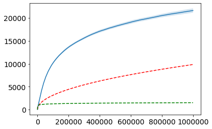
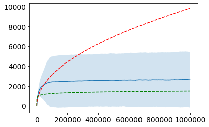
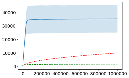
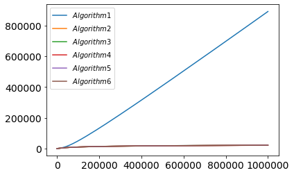
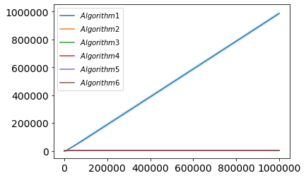
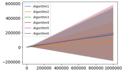
Table 1: Regret for corralling when $\Delta_{i}=0.2$

Table 1 reports the regret (top) and number of plays of each algorithm found in our experiments when $\Delta_{i}=0.2$. The plots represent the average regret, in blue, and the average number of pulls of each algorithm (color according to the legend) over $75$ runs of each experiment. The standard deviation is represented by the shaded blue region. The algorithm that contains the optimal arm is $\mathcal{A}_{1}$ and is an instance of UCB-I. The red dotted line in the top plots is given by $4\sqrt{KT}+\mathbb{E}[R_{1}(T)]$, and the green dotted line is given by $4\sum_{i\neq 1}\frac{k_{i}\operatorname{log}\left(T\right)}{\Delta_{i}}+\mathbb{E}[R_{1}(T)]$. These lines serve as a reference across experiments and we believe they are more accurate upper bounds for the regret of the proposed and existing algorithms. As expected, we see that, in the large gap regime, the Corral algorithm exhibits $\Omega(\sqrt{T})$ regret, while the regret of Algorithm 2 remains bounded in $O(\operatorname{log}\left(T\right))$. Algorithm 1 admits two regret phases. In the initial phase, its regret is linear, while in the second phase it is logarithmic. This is typical of UCB strategies in the stochastic MAB problem (Garivier et al., 2018b).

Small gap experiments

Corral	Algorithm 2	Algorithm 1

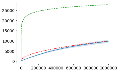
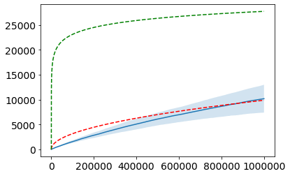
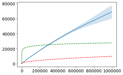
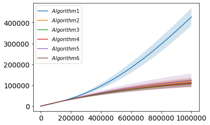
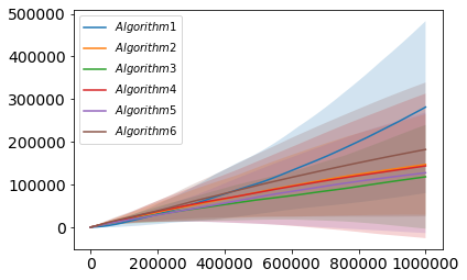
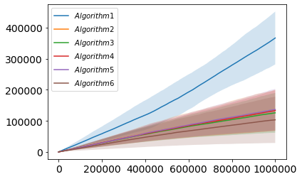
Table 2: Regret for corralling when $\Delta_{i}=0.02$

Table 2 reports the results of our experiments for $\Delta_{i}=0.02$. The setting of the experiments is the same as in the large gap case. We observe that both Corral and Algorithm 2 behave according to the $O(\sqrt{T})$ bounds. This is expected since, when $\Delta_{i}=0.02$, the optimistic bound dominates the $\sqrt{T}$-bound. The result for Algorithm 1 might be somewhat surprising, as its regret exceeds both the green and red lines. We emphasize that this experiment does not contradict Theorem 4.2. Indeed, if we were to plot the green and red lines according to the bounds of Theorem 4.2, the regret would remain below both lines.

Our experiments suggest that Algorithm 2 is the best corralling algorithm. A tighter analysis would potentially yield optimistic regret bounds in the order of $O\left(\sum_{i\neq i^{*}}\frac{k_{i}\operatorname{log}\left(T\right)}{\Delta_{i}}+\mathbb{E}[R_{i^{*}}(T)]\right)$. Furthermore, we expect that the bounds of Theorem 4.2 are tight. For more detailed experiments, we refer the reader to Appendix A.

7 Model selection for linear bandits

While the main focus of the paper is corralling MAB base learners when there exists a best overall base algorithm, we now demonstrate that several known model selection results can be recovered using Algorithm 2.

We begin by recalling the model selection problem for linear bandits. The learner is given access to a set of loss functions $\mathcal{F}\colon\mathcal{X}\times\mathcal{A}\rightarrow\mathbb{R}$ mapping from contexts $\mathcal{X}$ and actions $\mathcal{A}$ to losses. In the linear bandits setting, $\mathcal{F}$ is structured as a nested sequence of classes $\mathcal{F}_{1}\subseteq\mathcal{F}_{2}\subseteq\ldots\subseteq\mathcal{F}_{K}=\mathcal{F}$, where each $\mathcal{F}_{i}$ is defined as

$$\mathcal{F}_{i}=\{(x,a)\rightarrow\langle\beta_{i},\phi_{i}(x,a)\rangle:\beta_{i}\in\mathbb{R}^{d_{i}}\},$$

for some feature embedding $\phi_{i}\colon\mathcal{X}\times\mathcal{A}\rightarrow\mathbb{R}^{d_{i}}$. It is assumed that each feature embedding $\phi_{i}$ contains $\phi_{i-1}$ as its first $d_{i-1}$ coordinates. It is further assumed that there exists a smallest $i^{*}\leq K$ to which the optimal parameter $\beta^{*}$ belongs, that is the observed losses for each context-action pair $(x,a)$ satisfy $\ell_{t}(x,a)=\mathbb{E}\left[\langle\beta^{*},\phi_{d_{i^{*}}}(x,a)\rangle\right]$. The goal in the model selection problem is to identify $i^{*}$ and compete against the smallest loss for the $t$-th context in $\mathbb{R}^{d_{i^{*}}}$ by minimizing the regret:

$$R_{i^{*}}(T)=\sum_{t=1}^{T}\Big{(}\mathbb{E}[\langle\beta^{*},\phi_{i^{*}}(x_{t},a_{t})\rangle]$$

$$\hskip 100.0pt-\min_{a\in\mathcal{A}}\mathbb{E}[\langle\beta^{*},\phi_{i^{*}}(x_{t},a)\rangle]\Big{)},$$

where the expectation is with respect to all randomness in the sampling of the contexts $x_{t}\sim\mathcal{D}$, actions and additional noise. We adopt the standard assumption that, given $x_{t}$, the observed loss for any $a$ can be expressed as follows: $\langle\beta,\phi_{i}(x_{t},a)\rangle+\xi_{t}$, where $\xi_{t}$ is a zero-mean, sub-Gaussian random variable with variance proxy $1$ and for each of the context-action pairs it holds that $\langle\beta,\phi_{i}(x_{t},a)\rangle\in[0,1]$.

7.1 Algorithm and main result

We assume that there are $K$ base learners $\{\mathcal{A}_{i}\}_{i=1}^{K}$ such that the regret of $\mathcal{A}_{i}$, for $i\geq i^{*}$, is bounded by $\tilde{O}(d_{i}^{\alpha}\sqrt{T})$. That is, whenever the model is correctly specified, the $i$-th algorithm admits a meaningful regret guarantee. In the setting of Foster et al. (2019), $\mathcal{A}_{i}$ can be instantiated as LinUCB and in that case $\alpha=1/2$. Further, in the setting of infinite arms, $\mathcal{A}_{i}$ can be instantiated as OFUL (Abbasi-Yadkori et al., 2011), in which case $\alpha=1$. Both $\alpha=1/2$ and $\alpha=1$ govern the min-max optimal rates in the respective settings. Our algorithm is now a simple modification of Algorithm 2. At every time-step $t$, we update $\widehat{L}_{t}=\widehat{L}_{t-1}+\widehat{\ell}_{t}+\mathbf{d}$, where $\mathbf{d}_{i}=\frac{d_{i}^{2\alpha}}{\sqrt{T}}$. Intuitively, our modification creates a gap between the losses of $\mathcal{A}_{i^{*}}$ and any $\mathcal{A}_{i}$ for $i>i^{*}$ of the order $d_{i}^{2\alpha}$. On the other hand for any $i<i^{*}$, perturbing the loss can result in at most additional $d_{i^{*}}^{2\alpha}\sqrt{T}$ regret. With the above observations, the bound guaranteed by Theorem 5.2 implies that the modified algorithm should incur at most $\tilde{O}(d_{i^{*}}^{2\alpha}\sqrt{T})$ regret. In Appendix F, we show the following regret bound.

Theorem 7.1.

Assume that every base learner $\mathcal{A}_{i}$, $i\geq i^{*}$, admits a $\tilde{O}(d_{i}^{\alpha}\sqrt{T})$ regret. Then, there exists a corralling strategy with expected regret bounded by $\tilde{O}(d_{i^{*}}^{2\alpha}\sqrt{T}+K\sqrt{T})$. Moreover, under the additional assumption that the following holds for any $i<i^{*}$, for all $(x,a)\in\mathcal{X}\times\mathcal{A}$

$$\mathbb{E}[\langle\beta_{i},\phi_{i}(x,a)\rangle]-\min_{a\in\mathcal{A}}\mathbb{E}[\langle\beta^{*},\phi_{i^{*}}(x,a)\rangle]\geq 2\frac{d_{i^{*}}^{2\alpha}-d_{i}^{2\alpha}}{\sqrt{T}},$$

the expected regret of the same strategy is bounded as $\tilde{O}(d_{i^{*}}^{\alpha}\sqrt{T}+K\sqrt{T})$.

Typically, we have $K=O(\operatorname{log}\left(T\right))$ and thus Theorem 7.1 guarantees a regret of at most $\tilde{O}(d_{i^{*}}^{2\alpha}\sqrt{T})$. Furthermore, under a gap-assumption, which implies that the value of the smallest loss for the optimal embedding $i^{*}$ is sufficiently smaller compared to the value of any sub-optimal embedding $i<i^{*}$, we can actually achieve a corralling regret of the order $R_{i^{*}}(T)$. In particular, for the setting of Foster et al. (2019), our strategy yields the desired $\tilde{O}(\sqrt{d_{i^{*}}T})$ regret bound. Notice that the regret guarantees are only meaningful as long as $d_{i^{*}}=o(T^{1/(2\alpha)})$. In such a case, the second assumption on the gap is that the gap is lower bounded by $o(1)$. This is a completely problem-dependent assumption and in general we expect that it cannot be satisfied.

8 Conclusion

We presented an extensive analysis of the problem of corralling stochastic bandits. Our algorithms are applicable to a number of different contexts where this problem arises. There are also several natural extensions and related questions relevant to our study. One natural extension is the case where the set of arms accessible to the base algorithms admit some overlap and where the reward observed by one algorithm could serve as side-information to another algorithm. Another extension is the scenario of corralling online learning algorithms with feedback graphs. In addition to these and many other interesting extensions, our analysis may have some connection with the study of other problems such as model selection in contextual bandits (Foster et al., 2019) or active learning.

Appendix A Additional experiments

We now provide more detailed plots for our experiments, including number of times each corralled algorithm has been played and the distribution over corralled distribution each of the corralling algorithm keeps (in the case of Algorithm 1 this is just the empirical distribution of played algorithms). We additionally present experiments in which the corralled algorithm containing the best arm is FTRL with $\frac{1}{2}$-Tsallis entropy regularization and Thompson sampling.

Detailed experimental setup.

The algorithms which we corral are UCB-I, Thompson sampling (TS), and FTRL with $\frac{1}{2}$-Tsallis entropy reguralizer (Tsallis-INF). We chose these algorithms as they all come with regret guarantees for the stochastic multi-armed problem and they broadly represent three different classes of algorithms, i.e, algorithms based on the optimism in the face of uncertainty principle, algorithms based on posterior sampling, and algorithms based on online mirror descent. As already discussed in Section 6, when implementing Algorithm 2 and Corral, we never restart the corralled algorithms and run them with their default parameters. Even though, there are no theoretical guarantees for this modification of the corralling algorithms, we will see that the regret bounds remain meaningful in practice. In all of the experiments we corral two instances of UCB-I, TS, and FTRL for a total of six algorithms. The best algorithm plays over 10 arms. Every other algorithm plays over 5 arms. Intuitively, the higher the number of arms implies higher complexity of the best algorithm which would lead to higher regret and a harder corralling problem. The rewards for each algorithm are Bernoulli random variables setup according to the following parameters: base_reward, in_gap, out_gap, and low_reward. The best overall arm has expected reward $\textsc{base\_reward}+\textsc{in\_gap}+\textsc{out\_gap}$. Every other arm of Algorithm 1 has expected reward equal to low_reward. For all other algorithms the best arm has reward $\textsc{base\_reward}+\textsc{in\_gap}$ and other arms have reward base_reward. In all of the experiments we set $\textsc{base\_reward}=0.5,\textsc{in\_gap}=0.01,\textsc{low\_reward}=0.2$. While a small in_gap implies a large regret for the algorithms containing sub-optimal arms, it also reduces the likelihood that said algorithms would have small average reward. Combined with setting $\textsc{low\_reward}=0.2$, this will make the average reward of $\mathcal{A}_{1}$ look small in the initial number of rounds, compared to the average reward of $\mathcal{A}_{i},i>1$ and hence makes the corralling problem harder. We run two set of experiments, an easy set for which $\textsc{out\_gap}=0.19$, which translates to gaps $\Delta_{i}=0.2$ in our regret bounds, and a hard set for which $\textsc{out\_gap}=0.01$ which implies $\Delta_{i}=0.02$. Finally time horizon is set to $T=1000000$.

A.1 UCB-I contains best arm

Experiments can be found in Figure 1 for $\Delta_{i}=0.2$ and in Figure 2 for $\Delta_{i}=0.02$.

(a) Corral regret

(b) Corral number of pulls

(c) Corral distribution

(d) Algorithm 2 regret

(e) Algorithm 2 number of pulls

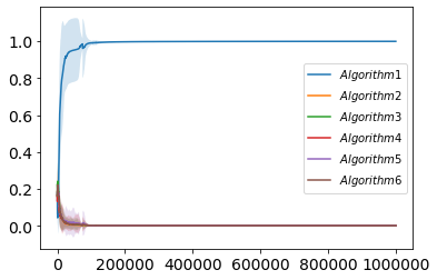
(f) Algorithm 2 distribution

(g) Algorithm 1 regret

(h) Algorithm 1 number of pulls

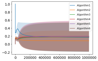
(i) Algorithm 1 distribution

Figure 1: UCB-I contains best arm,$\Delta_{i}=0.2,\textsc{ALG}_{1:2}=\textsc{UCB-I},\textsc{ALG}_{3:4}=\textsc{Tsallis-INF},\textsc{ALG}_{5:6}=\textsc{TS}$.

(a) Corral regret

(b) Corral number of pulls

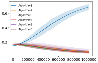
(c) Corral distribution

(d) Algorithm 2 regret

(e) Algorithm 2 number of pulls

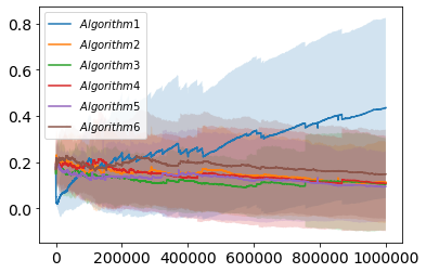
(f) Algorithm 2 distribution

(g) Algorithm 1 regret

(h) Algorithm 1 number of pulls

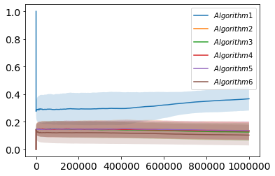
(i) Algorithm 1 distribution

Figure 2: UCB-I contains best arm,$\Delta_{i}=0.02,\textsc{ALG}_{1:2}=\textsc{UCB-I},\textsc{ALG}_{3:4}=\textsc{Tsallis-INF},\textsc{ALG}_{5:6}=\textsc{TS}$.

A.2 Tsallis-INF contains best arm

Experiments can be found in Figure 3 for $\Delta_{i}=0.2$ and in Figure 4 for $\Delta_{i}=0.02$.

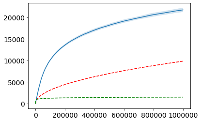
(a) Corral regret

(b) Corral number of pulls

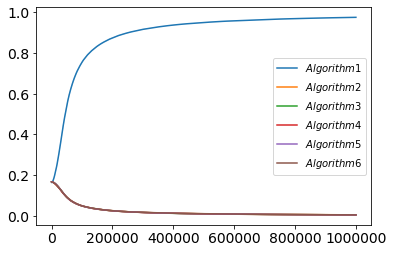
(c) Corral distribution

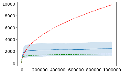
(d) Algorithm 2 regret

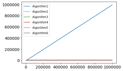
(e) Algorithm 2 number of pulls

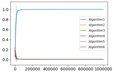
(f) Algorithm 2 distribution

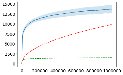
(g) Algorithm 1 regret

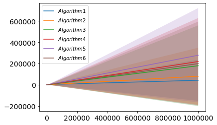
(h) Algorithm 1 number of pulls

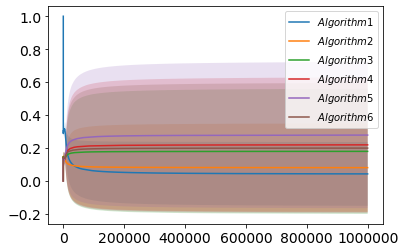
(i) Algorithm 1 distribution

Figure 3: Tsallis-INF contains best arm,$\Delta_{i}=0.2,\textsc{ALG}_{1:2}=\textsc{Tsallis-INF},\textsc{ALG}_{3:4}=\textsc{UCB-I},\textsc{ALG}_{5:6}=\textsc{TS}$.

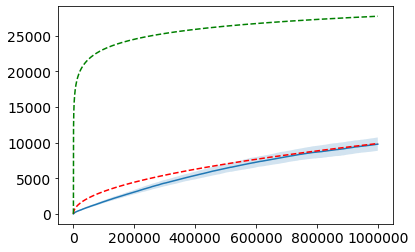
(a) Corral regret

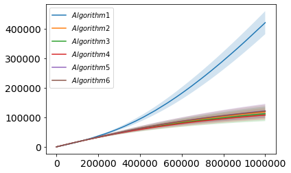
(b) Corral number of pulls

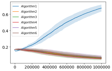
(c) Corral distribution

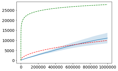
(d) Algorithm 2 regret

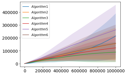
(e) Algorithm 2 number of pulls

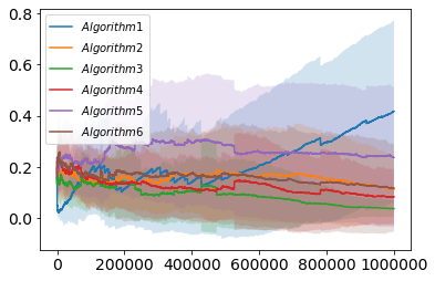
(f) Algorithm 2 distribution

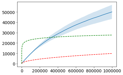
(g) Algorithm 1 regret

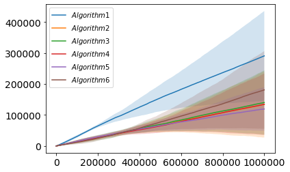
(h) Algorithm 1 number of pulls

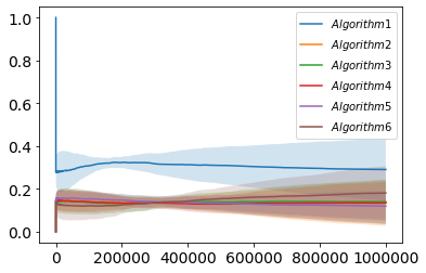
(i) Algorithm 1 distribution

Figure 4: Tsallis-INF contains best arm,$\Delta_{i}=0.02,\textsc{ALG}_{1:2}=\textsc{Tsallis-INF},\textsc{ALG}_{3:4}=\textsc{UCB-I},\textsc{ALG}_{5:6}=\textsc{TS}$.

A.3 Thompson sampling contains best arm

Experiments can be found in Figure 5 for $\Delta_{i}=0.2$ and in Figure 6 for $\Delta_{i}=0.02$.

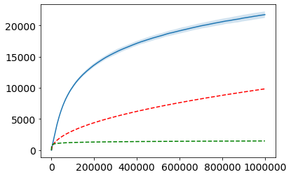
(a) Corral regret

(b) Corral number of pulls

(c) Corral distribution

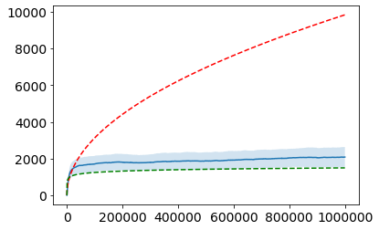
(d) Algorithm 2 regret

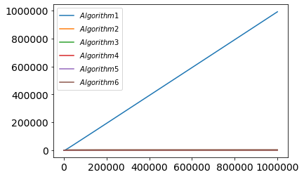
(e) Algorithm 2 number of pulls

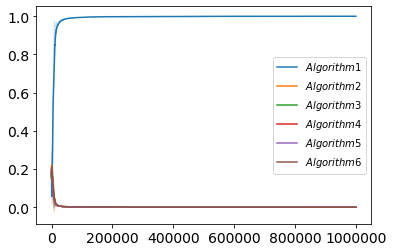
(f) Algorithm 2 distribution

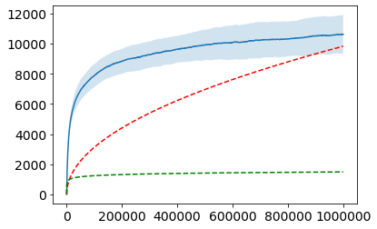
(g) Algorithm 1 regret

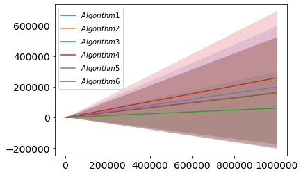
(h) Algorithm 1 number of pulls

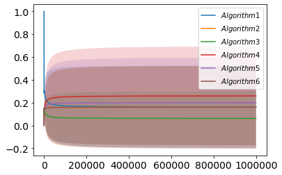
(i) Algorithm 1 distribution

Figure 5: Thompson sampling (TS) contains best arm,$\Delta_{i}=0.2,\textsc{ALG}_{1:2}=\textsc{TS},\textsc{ALG}_{3:4}=\textsc{UCB-I},\textsc{ALG}_{5:6}=\textsc{Tsallis-INF}$.

(a) Corral regret

(b) Corral number of pulls

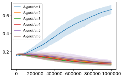
(c) Corral distribution

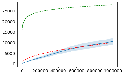
(d) Algorithm 2 regret

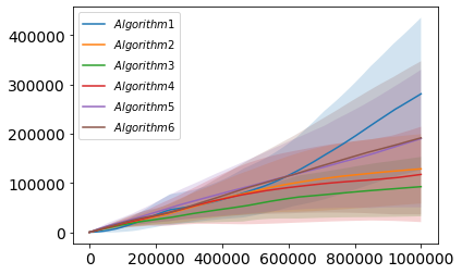
(e) Algorithm 2 number of pulls

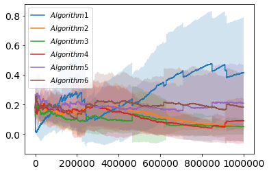
(f) Algorithm 2 distribution

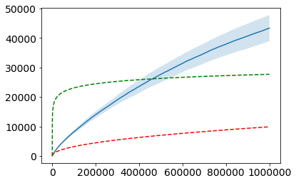
(g) Algorithm 1 regret

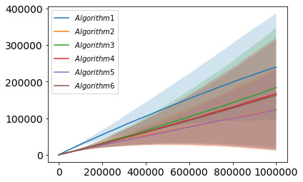
(h) Algorithm 1 number of pulls

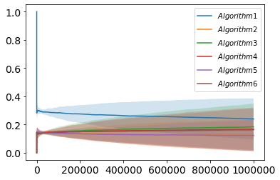
(i) Algorithm 1 distribution

Figure 6: TS contains best arm,$\Delta_{i}=0.02,\textsc{ALG}_{1:2}=\textsc{TS},\textsc{ALG}_{3:4}=\textsc{UCB-I},\textsc{ALG}_{5:6}=\textsc{Tsallis-INF}$.

Appendix B Proofs from Section 3

We first introduce the formal construction briefly described in Section 3.

B.1 First lower bound

Assume that the corralling algorithm can play one of two algorithms, $\mathcal{A}_{1}$ or $\mathcal{A}_{2}$, with the rewards of each arm played by these algorithms distributed according to a Bernoulli random variable. Algorithm $\mathcal{A}_{1}$ plays a single arm with expected reward $\mu_{1}$ and algorithm $\mathcal{A}_{2}$ is defined as follows.

Let $\beta$ be drawn according to the Bernoulli distribution $\beta\sim\text{Ber}(\frac{1}{2})$ and let $\alpha$ be drawn uniformly over the unit interval, $\alpha\sim\text{Unif}[0,1]$. If $\beta=1$, $\mathcal{A}_{2}$ alternates between playing an arm with mean $\mu_{2}$ and an arm with mean $\mu_{3}$ every round, so that the algorithm incurs linear regret. We set $\mu_{i}$s such that $\mu_{2}>\mu_{1}>\frac{\mu_{2}+\mu_{3}}{2}$. If $\beta=0$, then $\mathcal{A}_{2}$ behaves in the same way as if $\beta=1$ for the first $T^{(1-\alpha)}$ rounds and for the remaining $T-T^{(1-\alpha)}$ rounds $\mathcal{A}_{2}$ only pulls the arm with mean $\mu_{2}$. Notice that, in this setting, $\mathcal{A}_{2}$ admits sublinear regret almost surely.

We denote by $\mathbb{P}(\cdot|r_{1}(a_{i_{1},j_{1}}),\ldots,r_{t}(a_{i_{t},j_{t}}),\beta=i)$ the natural measure on the $\sigma$-algebra generated by the observed rewards under the environment $\beta=i$ and all the randomness of the player’s algorithm. To simplify the notation, we denote by $r_{1:t}$ the sequence $\{r_{s}(a_{i_{s},j_{s}})\}_{s=1}^{t}$. Let $N$ denote the random variable counting the number of times the corralling strategy selected $\mathcal{A}_{1}$. Information-theoretically, the player can obtain a good approximation of $\mu_{1}$ in time $O(\operatorname{log}\left(T\right))$ and, therefore, for simplicity, we assume that the player knows $\mu_{1}$ exactly. Note that this can only make the problem easier for the player. Given this information, we can assume that the player begins by playing algorithm $\mathcal{A}_{2}$ for $T-N+1$ rounds and then switches to $\mathcal{A}_{1}$ for the rest of the game. In particular, we assume that $T-N+1$ is the time when the player can figure out that $\beta=1$. We note that at time $T^{(1-\alpha)}$ we have $\mathbb{P}(\cdot|r_{1:T^{(1-\alpha)}},\beta=1)=\mathbb{P}(\cdot|r_{1:T^{(1-\alpha)}},\beta=0)$, as the distribution of the rewards provided by $\mathcal{A}_{2}$ do not differ between $\beta=1$ and $\beta=0$. Furthermore, any random strategy would also need to select algorithm $\mathcal{A}_{2}$ at least $T^{(1-\alpha)}+1$ rounds before it is able to distinguish between $\beta=1$ or $\beta=0$. It is also important to note that under the event that $\beta=1$, the corralling algorithm does not receive any information about the value of $\alpha$. This allows us to show that in the setting constructed above, with at least constant probability the best algorithm i.e., $\mathcal{A}_{1}$ when $\beta=1$ and $\mathcal{A}_{2}$ when $\beta=0$, has sublinear regret. Finally, a direct computation of the regret of this corralling strategy gives the following result.

Theorem B.1.

Let algorithms $\mathcal{A}_{1}$ and $\mathcal{A}_{2}$ follow the construction in Section 3. Then, with probability at least $1/2$ over the random choice of $\alpha$, any corralling strategy incurs regret at least $\tilde{\Omega}(T)$, while the regret of the best algorithm is at most $O(\sqrt{T})$.

Proof.

Let $R(T)$ denote the regret of the corralling algorithm. Direct computation shows that if $\beta=1$ the corralling regret is

$$\mathbb{E}[R(T)|\beta=1,r_{1:T^{(1-\alpha)}},\alpha]=\mathbb{E}\left[\left(\mu_{1}-\frac{\mu_{2}+\mu_{3}}{2}\right)(T-N)|\beta=1,r_{1:T^{(1-\alpha)}},\alpha\right]$$

Further if $\beta=0$ and $\mathcal{A}_{2}$ is the best algorithm the regret of corralling is

$$\mathbb{E}[R(T)|\beta=0,r_{1:T^{(1-\alpha)}},\alpha]=\mathbb{E}\left[T^{(1-\alpha)}\mu_{2}+(T-T^{(1-\alpha)})\mu_{2}|\beta=0,r_{1:T^{(1-\alpha)}},\alpha\right]$$

$$\geq \mathbb{E}\left[\frac{\mu_{2}+\mu_{3}}{2}T^{(1-\alpha)}+\mu_{2}(T-T^{(1-\alpha)})\right.$$

$$- \left.\mu_{1}N-\chi_{(N\leq T-T^{(1-\alpha)})}\left(\frac{\mu_{2}+\mu_{3}}{2}T^{(1-\alpha)}+\mu_{2}(T-T^{(1-\alpha)}-N)\right)\right.$$

$$- \left.\chi_{(N>T-T^{(1-\alpha)})}\frac{\mu_{2}+\mu_{3}}{2}(T-N)|\beta=0,r_{1:T^{(1-\alpha)}},\alpha\right],$$

where the characteristic functions describe the event in which we pull $\mathcal{A}_{1}$ less times than is needed for $\mathcal{A}_{2}$ to switch to playing the best action. Notice that the total regret for corralling is at least the above as we also need to add the regret of the best algorithm to the above.

We first consider the case $\beta=1$. Notice that in this case the corralling algorithm does not receive any information about $\alpha$ because $\mathcal{A}_{2}$ alternates between $\mu_{2}$ and $\mu_{3}$ at all rounds. This implies $\mathbb{E}[R(T)|\beta=1,\alpha]=\mathbb{E}[R(T)|\beta=1]$. Condition on the event $N\leq T-T^{(1-\alpha)}$. We have

$$\mathbb{E}[R(T)|\beta=1,N\leq T-T^{(1-\alpha)},r_{1:T^{(1-\alpha)}},\alpha] =$$

$$\mathbb{E}[R(T)|\beta=1,N\leq T-T^{(1-\alpha)},r_{1:T^{(1-\alpha)}}] \geq\left(\mu_{1}-\frac{\mu_{2}+\mu_{3}}{2}\right)\mathbb{E}[T^{(1-\alpha)}|\beta=1]$$

$$=\left(\mu_{1}-\frac{\mu_{2}+\mu_{3}}{2}\right)\mathbb{E}[T^{(1-\alpha)}]$$

$$=\left(\mu_{1}-\frac{\mu_{2}+\mu_{3}}{2}\right)\frac{T-1}{\operatorname{log}\left(T\right)},$$

where in the first inequality we have replaced $N$ by $T-T^{1-\alpha}$. Next consider the case $\beta=0$. Condition on the event $N>T-T^{(1-\alpha)}$. We have

$$\mathbb{E}[R(T)|\beta=0,N>T-T^{(1-\alpha)},r_{1:T^{(1-\alpha)}},\alpha]$$

$$=\mathbb{E}\left[\frac{\mu_{2}-\mu_{3}}{2}(T-T^{(1-\alpha)})-\left(\mu_{1}-\frac{\mu_{2}+\mu_{3}}{2}\right)N|\beta=0,N>T-T^{(1-\alpha)},r_{1:T^{(1-\alpha)}},\alpha\right]$$

$$\geq\mathbb{E}\left[(\mu_{2}-\mu_{1})T-\frac{\mu_{2}}{2}T^{(1-\alpha)}|\beta=0,N>T-T^{(1-\alpha)},r_{1:T^{(1-\alpha)}},\alpha\right]$$

$$=\mathbb{E}\left[(\mu_{2}-\mu_{1})T-\frac{\mu_{2}}{2}T^{1-\alpha}|\alpha\right],$$

where in the inequality we have used the fact that $N>T-T^{1-\alpha}$ to bound $-\mu_{1}N$ and $T\geq N$ to bound $\frac{\mu_{1}+\mu_{3}}{2}N$. Let $A$ denote the event $N\leq T-T^{(1-\alpha)}$. We are now ready to lower bound the regret of the player’s strategy as follows.

$$\mathbb{E}\left[R(T)|\alpha\right] =\frac{1}{2}\mathbb{E}\left[\mathbb{E}[R(T)|r_{1:T^{(1-\alpha)}},\beta=1,\alpha]+\mathbb{E}[R(T)|r_{1:T^{(1-\alpha)}},\beta=0,\alpha]|\alpha\right]$$

$$\geq\frac{1}{2}\mathbb{E}\left[\mathbb{P}(A|r_{1:T^{(1-\alpha)}},\beta=1,\alpha)\mathbb{E}[R(T)|r_{1:T^{(1-\alpha)}},\beta=1,A,\alpha]\right.$$

$$\left.+\mathbb{P}(A^{c}|r_{1:T^{(1-\alpha)}},\beta=1,\alpha)\mathbb{E}[R(T)|r_{1:T^{(1-\alpha)}},\beta=0,A^{c},\alpha]|\alpha\right]$$

$$\geq\frac{1}{2}\mathbb{E}\left[\mathbb{P}(A|r_{1:T^{(1-\alpha)}},\beta=1,\alpha)\left(\mu_{1}-\frac{\mu_{2}+\mu_{3}}{2}\right)\frac{T-1}{2\operatorname{log}\left(T\right)}\right.$$

$$\left.+(1-\mathbb{P}(A|r_{1:T^{(1-\alpha)}},\beta=1),\alpha)(\mu_{2}-\mu_{1})T-\frac{\mu_{2}}{2}T^{1-\alpha}|\alpha\right],$$

where in the first inequality we have used the fact that the conditional measures induced by $\beta=1$ and $\beta=0$ are equal for the first $T^{1-\alpha}$ rounds. Because $\alpha\geq 1/2$ with probability at least $1/2$ it holds that the random variable $\mathbb{E}[R(T)|\alpha]>\tilde{\Omega}(T)$ with probability at least $1/2$ and that the regret of $\mathcal{A}_{2}$ when $\beta=1$ is at most $O(\sqrt{T})$. ∎

B.2 A realistic setting for Algorithm 2

The behavior of $\mathcal{A}_{2}$ for the setting given by $\beta=0$, in the construction above, may seem somewhat artificial: a stochastic bandit algorithm may not be expected to behave in that manner when the gap between $\mu_{2}$ and $\mu_{3}$ is large enough. Here, we describe how to set $\mu_{1}$, $\mu_{2}$ and $\mu_{3}$ such that the successive elimination algorithm (Even-Dar et al., 2002) admits a similar behavior to $\mathcal{A}_{2}$ with $\beta=0$. Recall that successive elimination needs at least $1/\Delta^{2}$ rounds to distinguish between the arm with mean $\mu_{2}$ and the arm with mean $\mu_{3}$. In other words, for at least $1/\Delta^{2}$ rounds, it will alternate between the two arms. Therefore, we set $\frac{1}{\Delta^{2}}=T^{(1-\alpha)}$ or, equivalently, $\Delta=\frac{1}{T^{(1-\alpha)/2}}$, and $\mu_{1}=\mu_{2}-\frac{1}{4T^{(1-\alpha)/2}}$ to yield behavior similar to $\mathcal{A}_{2}$. For this construction, we show the following lower bound.

Theorem B.2 (Theorem 3.1 formal).

Let algorithms $\mathcal{A}_{1}$ and $\mathcal{A}_{2}$ follow the construction in Section B.2. With probability at least $1/4$ over the random choice of $\alpha$ any corralling strategy will incur regret at least $\tilde{\Omega}(\sqrt{T})$ while the gap between $\mu_{2}$ and $\mu_{3}$ is such that $\Delta>\omega(T^{-1/4})$ and hence the regret of the best algorithm is at most $o(T^{1/4})$.

Proof.

From the proof of Theorem B.1 we can compute, when $\beta=1$, we can directly compute

$$\mathbb{E}\left[R(T)|\beta=1,N\leq T-T^{(1-\alpha)},r_{1:T^{(1-\alpha)}},\alpha\right]$$

$$\geq \mathbb{E}\left[\left(\mu_{1}-\frac{\mu_{2}+\mu_{3}}{2}\right)T^{(1-\alpha)}|\beta=1,N\leq T-T^{(1-\alpha)},r_{1:T^{(1-\alpha)}},\alpha\right]$$

$$= \mathbb{E}\left[\frac{1}{4T^{(1-\alpha)/2}}T^{(1-\alpha)}|\beta=1,N\leq T-T^{(1-\alpha)},r_{1:T^{(1-\alpha)}}\right]=\frac{\sqrt{T}-1}{2\operatorname{log}\left(T\right)},$$

Where in the equality we again used the fact that if $\beta=1$, the corralling algorithm receives no information about $\alpha$. Further when $\beta=0$ we have

$$\mathbb{E}\left[R(T)|\beta=0,N>T-T^{(1-\alpha)},r_{1:T^{(1-\alpha)}}(a_{T^{(1-\alpha)}}),\alpha\right]$$

$$\geq \mathbb{E}\left[(\mu_{2}-\mu_{1})T-\frac{\mu_{2}}{2}T^{(1-\alpha)}|\beta=0,N>T-T^{(1-\alpha)},r_{1:T^{(1-\alpha)}},\alpha\right]$$

$$= \mathbb{E}\left[\frac{T^{(1+\alpha)/2}}{4}|\alpha\right]-\mathbb{E}\left[\frac{T^{(1-\alpha)}}{2}|\alpha\right].$$

Again we note that with probability $1/2$ we have $\alpha\geq 1/2$ and the above expression becomes asymptotically larger than $\sqrt{T}$. The same computation as in the proof of Theorem B.1 finishes the proof. ∎

We note that, in our construction, if $\beta=1$, then the inequality $\Delta\gg\frac{1}{\sqrt{T}}$ holds almost surely. In this setting, the instance-dependent regret bound for $\mathcal{A}_{2}$ and successive elimination is asymptotically smaller compared to the worst-case instance-independent regret bounds for stochastic bandit algorithms, which scale as $\tilde{O}(\sqrt{T})$ with the time horizon. This suggests that, even though $\mathcal{A}_{2}$ enjoys asymptotically better regret bounds than $\tilde{O}(\sqrt{T})$, the corralling algorithm will necessarily incur $\tilde{\Omega}(\sqrt{T})$ regret.

B.3 A lower bound when a worst case regret bound is known

Next, suppose that we know a worst case regret bound of $R_{2}(T)$ for algorithm $\mathcal{A}_{2}$. As before, we sample $\beta$ according to a Bernoulli distribution. If $\beta=1$, then algorithm $\mathcal{A}_{2}$ has a single arm with reward distributed as $\text{Ber}((\mu_{2}+\mu_{3})/2)$; in that case, $\mathcal{A}_{2}$ admits a regret equal to $0$. If $\beta=0$, then $\mathcal{A}_{2}$ has two arms distributed according to $\text{Ber}(\mu_{2})$ and $\text{Ber}(\mu_{3})$, respectively. We sample $\alpha\sim\text{Unif}[0,1]$, and let $\mathcal{A}_{2}$ play an arm uniformly at random for the first $R_{2}(T)^{(1-\alpha)}$ rounds. In particular, during each of the first $R_{2}(T)^{(1-\alpha)}$ rounds, $\mathcal{A}_{2}$ plays with equal probability the arm with mean $\mu_{2}$ and the arm with mean $\mu_{3}$. On round $R_{2}(T)^{(1-\alpha)}$, the algorithm switches to playing $\mu_{1}$ until the rest of the game. Notice that the rewards up to time $R_{2}(T)^{(1-\alpha)}$, whether $\beta=1$ or $\beta=0$, have the same distribution. Hence, $\mathbb{P}(\cdot|r_{1:R_{2}(T)^{(1-\alpha)}},\beta=1)=\mathbb{P}(\cdot|r_{1:R_{2}(T)^{(1-\alpha)}},\beta=0)$. Then, following the arguments in the proof of Theorem B.1, we can prove the following lower bound.

Theorem B.3.

Let algorithms $\mathcal{A}_{1}$ and $\mathcal{A}_{2}$ follow the construction in Section B.3. Suppose that the worst case known regret bound for Algorithm is $R_{2}(T)$. With probability at least $1/2$ over the random choice of $\alpha$ any corralling strategy will incur regret at least $\tilde{\Omega}(R_{2}(T))$ while the regret of $\mathcal{A}_{2}$ is at most $O(\sqrt{R_{2}(T)})$.

Appendix C Proofs from Section 4

Lemma C.1.

Suppose we run $2\operatorname{log}\left(1/\delta\right)$ copies of algorithm $\mathcal{A}_{i}$ which satisfies Equation 2. Let $\mathcal{A}_{med_{i}}$ denote the algorithm with median reward at time $t$. Then,

$$\mathbb{P}\left[t\mu_{med_{i},1}-\sum_{s=1}^{t}r_{s}(a_{med_{i},j_{s}})\geq 2\bar{R}_{med_{i}}(t)\right]\leq\delta.$$

Proof of Lemma 4.1.

First note that $\mu_{med_{i},1}=\mu_{i_{s},1}$ and $\bar{R}_{i_{s}}(t)=\bar{R}_{med_{i}}(t)$for all $s$ and $t$. The assumption in Equation 2 together with Markov’s inequality implies that for every copy $\mathcal{A}_{i_{s}}$ of $\mathcal{A}_{i}$ at time $t$ it holds that

$$\mathbb{P}\left[t\mu_{med_{i},1}-\sum_{s=1}^{t}r_{s}(a_{i,j_{s}})\geq 2\bar{R}_{med_{i}}(t)\right]\leq\frac{1}{2}.$$

Let $\mathcal{A}_{i_{1}},\ldots,\mathcal{A}_{i_{n}}$ be the algorithms which have reward smaller than $\mathcal{A}_{med_{i}}$ at time $t$. We have

$$\mathbb{P}\left[t\mu_{med_{i},1}-\sum_{s=1}^{t}r_{s}(a_{med_{i},j_{s}})\geq 2\bar{R}_{med_{i}}(t)\right] \leq\mathbb{P}\left[\bigcap_{l\in[n]}\left\{t\mu_{l,1}-\sum_{s=1}^{t}r_{s}(a_{i_{l},j_{s}})\geq 2\bar{R}_{med_{i}}(t)\right\}\right]$$

$$\leq\left(\frac{1}{2}\right)^{\operatorname{log}\left(1/\delta\right)}\leq\delta,$$

where the first inequality follows from the definition of $\mathcal{A}_{med_{i}}$ and $\mathcal{A}_{i_{l}}$ for $l\in[n]$. ∎

Theorem C.2.

Suppose that algorithms $\mathcal{A}_{1},\ldots,\mathcal{A}_{k}$ satisfy the following regret bound $\mathbb{E}[R_{i}(t)]\leq\sqrt{\alpha k_{i}t\operatorname{log}\left(t\right)}$. Then after $T$ rounds, Algorithm 1 produces a sequence of actions $a_{1},\ldots,a_{T}$, such that

$$T\mu_{1,1}-\mathbb{E}\left[\sum_{t=1}^{T}r_{t}(a_{i_{t},j_{t}})\right] \leq O\left(\sum_{i\neq i^{*}}\frac{k_{i}\operatorname{log}\left(T\right)^{2}}{\Delta_{i}}+\operatorname{log}\left(T\right)\mathbb{E}\left[R_{i^{*}}(T)\right]\right),$$

$$T\mu_{1,1}-\mathbb{E}\left[\sum_{t=1}^{T}r_{t}(a_{i_{t},j_{t}})\right] \leq O\left(\operatorname{log}\left(T\right)\sqrt{KT\operatorname{log}\left(T\right)\max_{i\in[K]}(k_{i})}\right).$$

Proof of Theorem 4.2.

For simplicity we assume that $\lceil\operatorname{log}\left(T\right)\rceil=\operatorname{log}\left(T\right)$. For the rest of the proof we let $t_{\ell}=T_{\ell}(t)$ to simplify notation. Further, since $\bar{R}_{\ell_{s}}=\bar{R}_{\ell},\forall s\in[\operatorname{log}\left(T\right)]$, we use $\bar{R}_{\ell}$ as the upper bound on the regret for all algorithms in $\mathbb{A}_{\ell}$. Let $\psi_{\ell}(t)=2\sqrt{\frac{2\operatorname{log}\left(t\right)}{t_{\ell}}}+\frac{\sqrt{2\bar{R}_{\ell}(t_{\ell})}}{t_{\ell}}$. The proof follows the standard ideas behind analyses of UCB type algorithms. If at time $t$ algorithm $\ell\neq 1$ is selected then one of the following must hold true:

$$\mu_{1,1}\geq\widehat{\mu}_{\bar{1}}(t_{1})+\frac{\sqrt{2\bar{R}_{1}(t_{1})}+\sqrt{2t_{1}\operatorname{log}\left(t\right)}}{t_{1}},$$ (5)

$$\widehat{\mu}_{med_{\ell}}(t_{\ell})>\mu_{1,1}+\sqrt{\frac{2\operatorname{log}\left(t\right)}{t_{\ell}}},$$ (6)

$$\Delta_{\ell}<2\sqrt{\frac{2\operatorname{log}\left(t\right)}{t_{\ell}}}+\frac{\sqrt{2\bar{R}_{\ell}(t_{\ell})}}{t_{\ell}}.$$ (7)

The above conditions can be derived by considering the case when the UCB for $\mathcal{A}_{1}$ is smaller than the UCB for $\mathcal{A}_{\ell}$ and every algorithm has been selected a sufficient number of times. Suppose that the three conditions above are false at the same time. Then we have

$$\widehat{\mu}_{\bar{1}}(t_{1}) +\frac{\sqrt{2\bar{R}_{1}(t_{1})}+\sqrt{2t_{1}\operatorname{log}\left(t\right)}}{t_{1}}>\mu_{1,1}=\mu_{1,\ell}+\Delta_{\ell}$$

$$\geq\Delta_{\ell}+\widehat{\mu}_{med_{\ell}}(t_{\ell})-\sqrt{\frac{2\operatorname{log}\left(t\right)}{t_{\ell}}}$$

$$\geq\widehat{\mu}_{med_{\ell}}(t_{\ell})+\frac{\sqrt{2\bar{R}_{\ell}(t_{\ell})}+\sqrt{2t_{\ell}\operatorname{log}\left(t\right)}}{t_{\ell}},$$

which contradicts the assumption that algorithm $\mathcal{A}_{\ell}$ was selected. With slight abuse of notation we use $[k_{\ell}]$ to denote the set of arms belonging to algorithm $\mathcal{A}_{\ell}$. Next we bound the expected number of times each sub-optimal algorithm is played up to time $T$. Let $\delta$ be an upper bound on the probability of the event that $\widehat{\mu}_{\bar{1}}(s)$ exceeds the UCB for $\mathcal{A}_{1}$.

$$\mathbb{E}[T_{\ell}] =\sum_{t=1}^{T}\mathbb{E}[\chi_{a_{i_{t},j_{t}}\in[k_{\ell}]}]\leq\psi_{\ell}^{-1}(\Delta_{\ell})+\sum_{t>\psi_{\ell}^{-1}(\Delta_{\ell})}\mathbb{P}\left[\text{Equation~{}\ref{eq:ucb_cond_1} or Equation~{}\ref{eq:ucb_cond_2} hold}\right]$$

$$\leq\psi_{\ell}^{-1}(\Delta_{\ell})+\sum_{t>\psi_{\ell}^{-1}(\Delta_{\ell})}\mathbb{P}\left[\exists s\in[t]:\mu_{1,1}\geq\widehat{\mu}_{\bar{1}}(s)+\frac{\sqrt{2\bar{R}_{1}(s)}+\sqrt{2s\operatorname{log}\left(t\right)}}{s}\right]$$

$$+\sum_{t>\psi_{\ell}^{-1}(\Delta_{\ell})}\mathbb{P}\left[\exists s\in[t]:\widehat{\mu}_{med_{\ell}}(s)>\mu_{1,1}+\sqrt{\frac{2\operatorname{log}\left(t\right)}{s}}\right]$$

$$\leq\sum_{t>\psi_{\ell}^{-1}(\Delta_{\ell})}t\delta+\sum_{t>\psi_{\ell}^{-1}(\Delta_{\ell})}\frac{1}{t}+\psi^{-1}(\Delta_{\ell}),$$

where the last inequality follows from the definition of $\delta$ and the fact that $\widehat{\mu}_{med_{\ell}}(s)\leq\widehat{\mu}_{med_{\ell},1}(s)$ (empirical mean of arm $1$ for algorithm $\mathcal{A}_{med_{\ell}}$ at time $s$) and the standard argument in the analysis of UCB-I. Setting $\delta=\frac{1}{T^{2}}$ finishes the bound on the number of suboptimal algorithm pulls. Next we consider bounding the regret incurred only by playing the median algorithms $\mathcal{A}_{med_{\ell}}$

$$t\mu_{1,1}-\mathbb{E}\left[\sum_{s=1}^{t}r_{s}(a_{i_{s},j_{s}})\right] =t\mu_{1,1}-\mathbb{E}\left[\sum_{\ell}t_{\ell}\mu_{\ell,1}+\sum_{\ell}\sum_{i}T_{med_{\ell},i}(t_{\ell})\mu_{\ell,i}-\sum_{\ell}t_{\ell}\mu_{\ell,1}\right]$$

$$=\mathbb{E}\left[\sum_{\ell\neq 1}t_{\ell}\Delta_{\ell}\right]+\sum_{\ell\neq 1}\mathbb{E}[R_{med_{\ell}}(t_{\ell})]+\mathbb{E}\left[R_{med_{1}}(t)\right]$$

$$\leq\sum_{\ell\neq 1}\Delta_{\ell}\psi^{-1}(\Delta_{\ell})+2\operatorname{log}\left(T\right)+\sum_{\ell\neq 1}\mathbb{E}[\sqrt{\alpha k_{\ell}t_{\ell}\operatorname{log}\left(t\right)}]+\mathbb{E}\left[R_{med_{1}}(t)\right]$$

$$\leq\sum_{\ell\neq 1}\Delta_{\ell}\psi^{-1}(\Delta_{\ell})+2\operatorname{log}\left(T\right)+\sum_{\ell\neq 1}\sqrt{\alpha k_{\ell}\mathbb{E}[t_{\ell}]\operatorname{log}\left(t\right)}+\mathbb{E}\left[R_{med_{1}}(t)\right]$$

$$\leq\sum_{\ell\neq 1}\Delta_{\ell}\psi^{-1}(\Delta_{\ell})+2\operatorname{log}\left(T\right)+\sum_{\ell\neq 1}\sqrt{\alpha k_{\ell}\psi^{-1}(\Delta_{\ell})\operatorname{log}\left(t\right)}$$

$$+\mathbb{E}\left[R_{med_{1}}(t)\right]+\sqrt{\alpha k_{\ell}}\operatorname{log}\left(t\right).$$

Now for the assumed regret bound on the algorithms, we have $\psi_{\ell}(t)=2\sqrt{\frac{2\operatorname{log}\left(t\right)}{t_{\ell}}}+\sqrt{2\frac{\alpha k_{\ell}\operatorname{log}\left(t_{\ell}\right)}{t_{\ell}}}$. This implies that $\psi_{\ell}^{-1}(\Delta_{\ell})\leq\frac{\alpha^{\prime}k_{\ell}\operatorname{log}\left(t\right)}{\Delta_{\ell}^{2}}$, for some other constant $\alpha^{\prime}$. To get the instance independent bound we first notice that by Jensen’s inequality we have

$$\sum_{\ell}\sqrt{\alpha^{\prime}k_{\ell}\mathbb{E}[t_{\ell}]\operatorname{log}\left(t\right)} \leq K\sqrt{\frac{1}{K}\sum_{\ell}\alpha^{\prime}\mathbb{E}[t_{\ell}]k_{\ell}\operatorname{log}\left(t\right)}$$

$$\leq\sqrt{\alpha^{\prime}Kt\operatorname{log}\left(t\right)\max_{\ell}(k_{\ell})}.$$

Next we can bound $\mathbb{E}\left[\sum_{\ell\neq 1}t_{\ell}\Delta_{\ell}\right]$ in the following way

$$\mathbb{E}\left[\sum_{\ell\neq 1}t_{\ell}\Delta_{\ell}\right] \leq\sum_{\ell}\Delta_{\ell}\sqrt{\mathbb{E}[t_{\ell}]}\sqrt{\mathbb{E}[t_{\ell}]}=\sum_{\ell}\sqrt{\Delta_{\ell}^{2}\mathbb{E}[t_{\ell}]}\sqrt{\mathbb{E}[t_{\ell}]}$$

$$=\sum_{\ell}\sqrt{\alpha^{\prime}k_{\ell}\mathbb{E}[t_{\ell}]\operatorname{log}\left(t\right)}\leq\sqrt{\alpha^{\prime}Kt\operatorname{log}\left(t\right)\max_{\ell}(k_{\ell})}$$

The theorem now follows. ∎

C.1 Proof of Theorem 4.3

Consider an instance of Algorithm 1, except that it runs a single copy of each base learner $\mathcal{A}_{i}$. Let $\mathcal{A}_{1}$ be a UCB algorithm with two arms with means $\mu_{1}>\mu_{2}$, respectively. The arm with mean $\mu_{1}$ is set according to a Bernoulli random variable, and the arm with mean $\mu_{2}$ is deterministic. Let algorithm $\mathcal{A}_{2}$ have a single deterministic arm with mean $\mu_{3}$, such that $\mu_{1}>\mu_{3}$ and $\mu_{3}>\mu_{2}$. Let $\Delta=\mu_{1}-\mu_{3}$. We now follow the lower bounding technique of Audibert et al. (2009).

Consider the event that in the first $q$ pulls of arm $a_{1}^{\mathcal{A}_{1}}$, we have $r_{t}(a_{1,1})=0$, i.e. $\mathscr{E}=\{r_{1}(a_{1,1})=0,r_{2}(a_{1,1})=0,\ldots,r_{q}(a_{1,1})=0\}$. This event occurs with probability $(1-\mu_{1})^{q}$. Notice that on event $\mathscr{E}$, the upper confidence bound for $\mu_{1}$ as per $\mathcal{A}_{1}$ is $\sqrt{\frac{\alpha\operatorname{log}\left(T_{1}(t)\right)}{q}}$ during time $t$. This implies that for $a_{1,1}$ to be pulled again we need $\sqrt{\frac{\alpha\operatorname{log}\left(T_{1}(t)\right)}{q}}>\mu_{2}$ and hence for the first $\operatorname{exp}\left(q\mu_{2}^{2}/\alpha\right)$ rounds in which $\mathcal{A}_{1}$ is selected by the corralling algorithm, $a_{1,1}$ is only pulled $q$ times. Further, on $\mathscr{E}$, the upper confidence bound for $\mathcal{A}_{1}$ as per the corralling algorithm is of the form $\sqrt{\frac{2\beta\operatorname{log}\left(t\right)}{T_{1}(t)}}$. This implies that for $\mathcal{A}_{1}$ to be selected again we need $\mu_{2}+\sqrt{\frac{2\beta\operatorname{log}\left(t\right)}{T_{1}(t)}}>\mu_{3}$. Let $\tilde{\Delta}=\mu_{3}-\mu_{2}$. Then, the above implies that in the first $t\leq\operatorname{exp}\left(T_{1}(t)\tilde{\Delta}^{2}/(2\beta)\right)$ rounds, $\mathcal{A}_{1}$ is pulled at most $T_{1}(t)$ times. Combining with the bound for the number of pulls of $a_{1,1}$ we arrive at the fact that on $\mathscr{E}$, $a_{1,1}$ can not be pulled more than $q$ times in the first $\operatorname{exp}\left(\frac{\tilde{\Delta}^{2}\operatorname{exp}\left(q\mu_{2}^{2}/\alpha\right)}{2\beta}\right)$ rounds. Let $q$ be large enough so that $q\leq\frac{1}{2}\operatorname{exp}\left(\frac{\tilde{\Delta}^{2}\operatorname{exp}\left(q\mu_{2}^{2}/\alpha\right)}{2\beta}\right)$. Then, for large enough $T$, we have that the pseudo-regret of the corralling algorithm is $\widehat{R}(T)\geq\frac{1}{2}\Delta\operatorname{exp}\left(\frac{\tilde{\Delta}^{2}\operatorname{exp}\left(q\mu_{2}^{2}/\alpha\right)}{2\beta}\right)$. Taking $q=\operatorname{log}\left(\frac{2\beta}{\tilde{\Delta}^{2}}\operatorname{log}\left(\tau\frac{\alpha}{\mu_{2}^{2}}\right)\right)$, we get

$$\mathbb{P}\left[\widehat{R}(T)\geq\frac{1}{2}\Delta\tau\right]\geq\mathbb{P}\left[\mathscr{E}\right]=(1-\mu_{1})^{q}=\frac{1}{\operatorname{exp}\left(q\right)^{\operatorname{log}\left(1/(1-\mu_{1})\right)}}=\Big{(}\frac{\tilde{\Delta}^{2}}{2\beta\operatorname{log}\left(\tau\right)}\Big{)}^{\frac{\alpha}{\mu_{2}^{2}}\operatorname{log}\left(1/(1-\mu_{1})\right)}.$$

Let $\gamma=\frac{\alpha}{\mu_{2}^{2}}\operatorname{log}\left(1/(1-\mu_{1})\right)$. We can now bound the expected pseudo-regret of the algorithm by integrating over $2\leq\tau\leq T$, to get

$$\mathbb{E}[\widehat{R}(T)] \geq\frac{1}{2}\Delta\int_{2}^{T}\Big{(}\frac{\tilde{\Delta}^{2}}{2\beta\operatorname{log}\left(\tau\right)}\Big{)}^{\frac{\alpha}{\mu_{2}^{2}}\operatorname{log}\left(1/(1-\mu_{1})\right)}d\tau=\frac{1}{2}\Delta\Big{(}\frac{\tilde{\Delta}^{2}}{2\beta}\Big{)}^{\gamma}\int_{2}^{T}\left(\frac{1}{\operatorname{log}\left(\tau\right)}\right)^{\gamma}d\tau$$

$$\geq\frac{1}{2}\Delta\Big{(}\frac{\tilde{\Delta}^{2}}{2\beta}\Big{)}^{\gamma}\frac{T-2}{\left(\operatorname{log}\left(\frac{T+2}{2}\right)\right)^{\gamma}},$$

where the last inequality follows from the Hermite-Hadamart inequality.

It is important to note that the above reasoning will fail if $\gamma$ is a function of $T$. This might occur if in the UCB for $\mathcal{A}_{1}$ we have $\alpha=\operatorname{log}\left(T\right)$. In such a case the lower bounds become meaningless as $\frac{1}{\operatorname{log}\left((T+2)/2\right)}^{\gamma}\leq o(1/T)$. Further, it should actually be possible to avoid boosting in this case as the tail bound of the regret will now be upper bounded as $\mathbb{P}[R_{1}(t)\geq\Delta\tau]\leq\frac{1}{T\tau^{c}}$.

General Approach if Regret has a Polynomial Tail.

Assume that, in general, the best algorithm has the following regret tail:

$$\mathbb{P}\left[R_{1}(t)\geq\frac{1}{2}\Delta_{1,1}\tau\right]\geq\frac{1}{\tau^{c}},$$

for some constant $c$. Results in Salomon and Audibert (2011) suggest that for stochastic bandit algorithms which enjoy anytime regret bounds we can not have a much tighter high probability regret bound. Let $\mathscr{E}_{T_{1}(t)}=\{R_{1}(T_{1}(t))\geq T_{1}(t)(\mu_{1}-\frac{1}{\sqrt{2}}\mu_{3})\}$. After $T_{1}(t)$ pulls of $\mathcal{A}_{1}$ the reward plus the UCB for $\mathcal{A}_{1}$ is at most $\frac{\sum_{s=1}^{T_{1}(t)}r_{s}(a_{1,j_{s}})}{T_{1}(t)}+\sqrt{\frac{\alpha k_{1}\operatorname{log}\left(t\right)}{T_{1}(t)}}$, and on $\mathscr{E}_{T_{1}(t)}$, we have $\frac{\sum_{s=1}^{T_{1}(t)}r_{s}(a_{1,j_{s}})}{T_{1}(t)}\leq\frac{1}{\sqrt{2}}\mu_{3}$. This implies that in the first $t$ rounds, $\mathcal{A}_{1}$ could not have been pulled more than

$$\frac{\alpha k_{1}\operatorname{log}\left(t\right)}{\left(\mu_{3}-\frac{\sum_{s=1}^{T_{1}(t)}r_{s}(a_{1,j_{s}})}{T_{1}(t)}\right)^{2}}\leq\frac{2\alpha k_{1}\operatorname{log}\left(t\right)}{\mu_{3}^{2}}.$$

Setting $T_{1}(t)=\frac{2\alpha k_{1}\operatorname{log}\left(T\right)}{\mu_{3}^{2}}$, we have that $\mathscr{E}_{T_{1}(t)}$ occurs with probability at least $\left(\frac{\Delta_{1,2}\mu_{3}^{2}}{4\alpha k_{1}\operatorname{log}\left(T\right)}\right)^{c}$ and hence the expected regret of the corralling algorithm is at least

$$\left(\frac{\Delta_{1,2}\mu_{3}^{2}}{4\alpha k_{1}\operatorname{log}\left(T\right)}\right)^{c}\Delta\left(T-\frac{2\alpha k_{1}\operatorname{log}\left(T\right)}{\mu_{3}^{2}}\right).$$

We have just showed the following.

Theorem C.3.

There exist instances $\mathcal{A}_{1}$ and $\mathcal{A}_{2}$ of UCB-I and a reward distribution, such that if Algorithm 1 runs a single copy of $\mathcal{A}_{1}$ and $\mathcal{A}_{2}$ the expected regret of the algorithm is at least

$$\mathbb{E}[R(T)]\geq\tilde{\Omega}(\Delta T).$$

Further, for any algorithm $\mathcal{A}_{1}$ such that $\mathbb{P}\left[R_{1}(t)\geq\frac{1}{2}\Delta_{1,1}\tau\right]\geq\frac{1}{\tau^{c}}$, there exists a reward distribution such that if Algorithm 1 runs a single copy of $\mathcal{A}_{1}$ the expected regret of the algorithm is at least

$$\mathbb{E}[R(T)]\geq\tilde{\Omega}((\Delta_{1,2})^{c}\Delta T).$$

Appendix D Proof of Theorem 5.2

D.1 Potential function and auxiliary lemmas

First we recall the definition of conjugate of a convex function $f$, denoted as $f^{*}$

$$f^{*}(y)=\max_{x\in\mathbb{R}^{d}}\langle x,y\rangle-f(x).$$

In our algorithm, we are going to use the following potential at time $t$

$$\Psi_{t}(w) =-4\sum_{i=1}^{K}\frac{\sqrt{w_{i}}-\frac{1}{2}w_{i}}{\eta_{t,i}}$$ (8)

$$\nabla\Psi_{t}(w)_{i} =-2\frac{\frac{1}{\sqrt{w_{i}}}-1}{\eta_{t,i}}$$

$$\nabla^{2}\Psi_{t}(w)_{i,i} =\frac{1}{w_{i}^{3/2}\eta_{t,i}},\nabla^{2}\Psi_{t}(w)_{i,j}=0$$

$$\nabla\Psi_{t}^{*}(Y)_{i} =\frac{1}{\left(-\frac{\eta_{t,i}}{2}Y_{i}+1\right)^{2}}$$

$$\Phi_{t}(Y) =\max_{w\in\Delta^{K-1}}\langle Y,w\rangle-\Psi_{t}(w)=\left(\Psi_{t}+\mathrm{I}_{\Delta^{K-1}}\right)^{*}(Y).$$

Further for a function $f$ we use $D_{f}(x,y)$ to denote the Bregman divergence between $x$ and $y$ induced by $f$ equal to

$$D_{f}(x,y)=f(x)-f(y)-\langle\nabla f(y),x-y\rangle=f(x)+f^{*}(\nabla f(y))-\langle\nabla f(y),x\rangle,$$

where the second inequality follows by the Fenchel duality equality $f^{*}(\nabla f(y))+f(y)=\langle\nabla f(y),y\rangle$. We now present a bandit algorithm is going to be the basis for the corralling algorithm. Let $\eta_{t}=\begin{pmatrix}\eta_{t,1}\\ \eta_{t,2}\\ \vdots\\ \eta_{t,K}\end{pmatrix}$ be the step size schedule for time $t$. The algorithm proceeds in epochs. Each epoch is twice as large as the preceding and the step size schedule remains non-increasing throughout the epochs, except when an OMD step is taken. In each epoch the algorithm makes a choice to either take two mirror descent steps, while increasing the step size:

$$\widehat{w}_{t+1} =\operatorname*{\rm argmin}_{w\in\Delta^{K-1}}\langle\widehat{\ell}_{t},w\rangle+D_{\Psi_{t}}(w,w_{t}),$$ (9)

$$\eta_{t+1,i} =\beta\eta_{t,i} \text{for $i:w_{t,i}\leq 1/\rho_{s_{i}}$},$$

$$\widehat{w}_{t+2} =\operatorname*{\rm argmin}_{w\in\Delta^{K-1}}\langle\widehat{\ell}_{t+1},w\rangle+D_{\Psi_{t+1}}(w,\widehat{w}_{t+1}),$$

$$\rho_{s_{i}} =2\rho_{s_{i}},$$

or the algorithm takes a FTRL step

$$w_{t+1}=\operatorname*{\rm argmin}_{w\in\Delta^{K-1}}\langle\widehat{L}_{t},w\rangle+\Psi_{t+1}(w),$$ (10)

where $\widehat{L}_{t}=\widehat{L}_{t-1}+\widehat{\ell}_{t}$ unless otherwise specified by the algorithm. We note that the algorithm can only increase the step size during the OMD step. For technical reasons we require a FTRL step after each OMD step. Further we require that the second step of each epoch be an OMD step, if there exists at least one $w_{t,i}\leq\frac{1}{\rho_{1}}$. The algorithm also can enter an OMD step during an epoch if at least one $w_{t,i}\leq\frac{1}{\rho_{n_{i}}}$. The intuition behind this behavior is as follows. Increasing the step size and doing an OMD step will give us negative regret during that round and we only require negative regret for a certain arm if the probability of pulling said arm becomes smaller than some threshold. The pseudo-code can be found in Algorithm 2. For the rest of the proofs and discussion we denote an iterate from the FTRL update as $w_{t}$ and an iterate from the OMD update as $\widehat{w}_{t}$. Further, intermediate iterates of OMD are denotes as $\tilde{w}_{t}$. We now present a couple of auxiliary lemmas useful for analyzing the OMD and FTRL updates.

Lemma D.1.

For any $x,y\in\Delta^{K-1}$ it holds

$$D_{\Psi_{t}}(x,y)=D_{\Phi_{t}}(\nabla\Phi_{t}^{*}(y),\nabla\Phi_{t}^{*}(x)).$$

Proof.

Since $\Psi_{t}+\mathrm{I}_{\Delta^{K-1}}$ is a convex, closed function on $\Delta^{K-1}$ it holds that $\Psi_{t}+\mathrm{I}_{\Delta^{K-1}}=((\Psi_{t}+\mathrm{I}_{\Delta^{K-1}})^{*})^{*}$ (see for e.g. (Brezis, 2010) Theorem 1.11). Further, $\Phi_{t}^{*}(x)=((\Psi_{t}+\mathrm{I}_{\Delta^{K-1}})^{*})^{*}(x)=\Psi_{t}(x)$. The above implies

$$D_{\Psi_{t}}(x,y)=D_{\Phi_{t}^{*}}(x,y)=D_{\Phi_{t}}(\nabla\Phi_{t}^{*}(y),\nabla\Phi_{t}^{*}(x)).$$

∎

Lemma D.2.

For any positive $\widehat{L}_{t}$ and $w_{t+1}$ generated according to update 10 we have

$$w_{t+1}=\nabla\Phi_{t+1}(-\widehat{L}_{t})=\nabla\Psi_{t+1}^{*}(-\widehat{L}_{t}+\nu_{t+1}\boldsymbol{1}),$$

for some scalar $\nu_{t}$. Further $(\widehat{L}_{t}-\nu_{t+1}\boldsymbol{1})_{i}>0$ for all $i\in[K]$.

Proof.

The proof is contained in Section 4.3 in Zimmert and Seldin (2018). ∎

Lemma D.3 (Lemma 16 Zimmert and Seldin (2018)).

Let $w\in\Delta^{K-1}$ and $\tilde{w}=\nabla\Psi_{t}^{*}(\nabla\Psi_{t}(w)-\ell)$. If $\eta_{t,i}\leq\frac{1}{4}$, then for all $\ell>-1$ it holds that $\tilde{w}_{i}^{3/2}\leq 2w_{i}^{3/2}$.

Algorithm 4 Corralling with Tsallis-INF

0:  Mult. constant $\beta$, thresholds $\{\rho_{i}\}_{i=1}^{n}$, initial step size $\eta$, epochs $\{\tau_{i}\}_{i=1}^{m}$, algorithms $\{\mathcal{A}_{i}\}_{i=1}^{K}$.

0:  Algorithm selection sequence $(i_{t})_{t=1}^{T}$.

1:  Initialize $t=1$, $w_{1}=Unif(\Delta^{K-1})$, $\eta_{1}=\eta$

2:  Initialize current threshold list $\theta\in[n]^{K}$ to $\bf 1$

3:  while $t\leq\operatorname{log}\left(T\right)+1$ 

4:     for $i\in[K]$ 

5:        Algorithm $i$ plays action $a_{i,j_{t}}$ and $\widehat{L}_{1,i}+=\ell_{t}(a_{i,j_{t}})$

6:     $t+=1$

7:  $t=2,w_{2}=\nabla\Phi_{2}(-\widehat{L}_{1}),1/\eta_{t+1}^{2}=1/\eta_{t}^{2}+1$

8:  while $j\leq m$ 

9:     for $t\in\tau_{j}$ 

10:        $\mathcal{R}_{t}=\emptyset$,$\widehat{\ell}_{t}=\texttt{PLAY-ROUND}(w_{t})$

11:        if $t$ is the first round of epoch $\tau_{j}$ and $\exists w_{t,i}\leq\frac{1}{\rho_{1}}$ 

12:           for $i\colon w_{t,i}\leq\frac{1}{\rho_{1}}$ 

13:              $\theta_{i}=\min\{s\in[n]\colon w_{t,i}>\frac{1}{\rho_{s}}\}$, $\mathcal{R}_{t}=\mathcal{R}_{t}\bigcup\{i\}$.

14:           $(w_{t+3},\widehat{L}_{t+2})=\texttt{NEG-REG-STEP}(w_{t},\widehat{\ell}_{t},\eta_{t},\mathcal{R}_{t},\widehat{L}_{t-1})$, $t=t+2$, $\widehat{\ell}_{t}=\texttt{PLAY-ROUND}(w_{t})$

15:        if $\exists i\colon w_{t,i}\leq\frac{1}{\rho_{\theta_{i}}}$ and prior step was not NEG-REG-STEP 

16:           for $i\colon w_{t,i}\leq\frac{1}{\rho_{\theta_{i}}}$ 

17:              $\theta_{i}+=1$, $\mathcal{R}_{t}=\mathcal{R}_{t}\bigcup\{i\}$.

18:           $(w_{t+3},\widehat{L}_{t+2})=\texttt{NEG-REG-STEP}(w_{t},\widehat{\ell}_{t},\eta_{t},\mathcal{R}_{t},\widehat{L}_{t-1})$, $t=t+2$, $\widehat{\ell}_{t}=\texttt{PLAY-ROUND}(w_{t})$

19:        else

20:           $1/\eta_{t+1}^{2}=1/\eta_{t}^{2}+1$, $w_{t+1}=\nabla\Phi_{t+1}(-\widehat{L}_{t})$

Algorithm 5 NEG-REG-STEP

0:  Previous iterate $w_{t}$, current loss $\widehat{\ell}_{t}$, step size $\eta_{t}$, set of rescaled step-sizes $\mathcal{R}_{t}$, cumulative loss $\widehat{L}_{t-1}$

0:  Plays two rounds of the game and returns distribution $w_{t+3}$ and cumulative loss $\widehat{L}_{t+2}$

1:  $(w_{t+1},\widehat{L}_{t})=\texttt{OMD-STEP}(w_{t},\widehat{\ell}_{t},\eta_{t},\mathcal{R}_{t},\widehat{L}_{t-1})$

2:  $\widehat{\ell}_{t+1}=\texttt{PLAY-ROUND}(w_{t+1})$, $\widehat{L}_{t+1}=\widehat{L}_{t}+\widehat{\ell}_{t+1}$

3:  for $i\in\mathcal{R}_{t}$ 

4:     $\eta_{t+2,i}=\beta\eta_{t,i}$ and restart $\mathcal{A}_{i}$ with updated environment $\theta_{i}=\frac{2}{w_{t,i}}$

5:  $w_{t+2}=\nabla\Phi_{t+2}(-\widehat{L}_{t+1})$

6:  $\widehat{\ell}_{t+2}=\texttt{PLAY-ROUND}(w_{t+2})$

7:  $\widehat{L}_{t+2}=\widehat{L}_{t+1}+\widehat{\ell}_{t+2},\eta_{t+3}=\eta_{t+2},t=t+2$

8:  $w_{t+1}=\nabla\Phi_{t+1}(-\widehat{L}_{t}),t=t+1$

Algorithm 6 OMD-STEP

0:  Previous iterate $w_{t}$, current loss $\widehat{\ell}_{t}$, step size $\eta_{t}$, set of rescaled step-sizes $\mathcal{R}_{t}$, cumulative loss $\widehat{L}_{t-1}$

0:  New iterate $w_{t+1}$, cumulative loss $\widehat{L}_{t}$

1:  $\nabla\Psi_{t}(\tilde{w}_{t+1})=\nabla\Psi_{t}(w_{t})-\widehat{\ell}_{t}$

2:  $w_{t+1}=\operatorname*{\rm argmin}_{w\in\Delta^{K-1}}D_{\Phi_{t}}(w,\tilde{w}_{t+1})$.

3:  $\mathrm{e}=\sum_{i\in\mathcal{R}_{t}}\mathrm{e}_{i}$

4:  $\tilde{L}_{t-1}=(\boldsymbol{1}_{k}-\mathrm{e})\odot(\widehat{L}_{t-1}-(\nu_{t-2}+\nu_{t-1})\boldsymbol{1}_{k})+\frac{1}{\beta}\mathrm{e}\odot((\widehat{L}_{t-1}-(\nu_{t-2}+\nu_{t-1})\boldsymbol{1}_{k}))$ // $\nu_{t-2}$ and $\nu_{t-1}$ are the Lagrange multipliers from the previous two FTRL steps.

5:  $\widehat{L}_{t}=\tilde{L}_{t-1}+\widehat{\ell}_{t}$

Algorithm 7 PLAY-ROUND

0:  Sampling distribution $w_{t}$

0:  Loss vector $\widehat{\ell}_{t}$

1:  Sample algorithm $i_{t}$ according to $\bar{w}_{t}=\left(1-\frac{1}{Tk}\right)w_{t}+\frac{1}{Tk}Unif(\Delta^{K-1})$.

2:  Algorithm $i_{t}$ plays action $a_{i_{t},j_{t}}$. Observe loss $\ell_{t}(a_{i_{t},j_{t}})$ and construct unbiased estimator $\widehat{\ell}_{t}=\frac{\ell_{t}(a_{i_{t},j_{t}})}{\bar{w}_{t,i_{t}}}\mathrm{e}_{i_{t}}$ of $\ell_{t}$.

3:  Give feedback to $i$-th algorithm as $\widehat{\ell}_{t}(a_{i,j_{t}})$, where $a_{i,j_{t}}$ was action provided by $\mathcal{A}_{i}$

D.2 Regret bound

We begin by studying the instantaneous regret of the FTRL update. The bound follows the one in Zimmert and Seldin (2018). Let $u=e_{i^{*}}$ be the unit vector corresponding to the optimal algorithm $\mathcal{A}_{i^{*}}$. First we decompose the regret into a stability term and a penalty term:

$$\langle\widehat{\ell}_{t},w_{t}-u\rangle =\langle\widehat{\ell}_{t},w_{t}\rangle+\Phi_{t}(-\widehat{L}_{t})-\Phi_{t}(-\widehat{L}_{t-1})\textit{ (Stability)}$$

$$-\Phi_{t}(-\widehat{L}_{t})+\Phi_{t}(-\widehat{L}_{t-1})-\langle\widehat{\ell}_{t},u\rangle\textit{ (Penalty)}.$$

The bound on the stability term follows from Lemma 11 in Zimmert and Seldin (2018), however, we will show this carefully, since parts of the proof will be needed to bound other terms. Recall the definition of $\Phi_{t}(Y)=\max_{w\in\Delta^{K-1}}\langle Y,w\rangle-\Psi_{t}(w)$. Since $w$ is in the simplex we have $\Phi_{t}(Y+\alpha\boldsymbol{1}_{k})=\max_{w\in\Delta^{K-1}}\langle Y,w\rangle+\langle\alpha\boldsymbol{1},w\rangle-\Psi_{t}(w)=\Phi_{t}(Y)+\alpha$. We also note that from Lemma D.2 it follows that we can write $\nabla\Psi_{t}(w_{t})=-\widehat{L}_{t-1}+\nu_{t}\boldsymbol{1}$. Combining the two facts we have

$$\langle\ell_{t},w_{t}\rangle+\Phi_{t}(-\widehat{L}_{t})-\Phi_{t}(-\widehat{L}_{t-1}) =\langle\ell_{t},w_{t}\rangle+\Phi_{t}(\nabla\Psi_{t}(w_{t})-\widehat{\ell}_{t}-\nu_{t}\boldsymbol{1})-\Phi_{t}(\nabla\Psi_{t}(w_{t})-\nu_{t}\boldsymbol{1})$$

$$=\langle\ell_{t}-\alpha\boldsymbol{1}_{k},w_{t}\rangle+\Phi_{t}(\nabla\Psi_{t}(w_{t})-\widehat{\ell}_{t}+\alpha\boldsymbol{1}_{k})-\Phi_{t}(\nabla\Psi_{t}(w_{t}))$$

$$\leq\langle\ell_{t}-\alpha\boldsymbol{1}_{k},w_{t}\rangle+\Psi_{t}^{*}(\nabla\Psi_{t}(w_{t})-\widehat{\ell}_{t}+\alpha\boldsymbol{1}_{k})-\Psi_{t}^{*}(\nabla\Psi_{t}(w_{t}))$$

$$=D_{\Psi_{t}^{*}}(\nabla\Psi_{t}(w_{t})-\widehat{\ell}_{t}+\alpha\boldsymbol{1}_{k},\nabla\Psi_{t}(w_{t}))$$

$$\leq\max_{z\in[\nabla\Psi_{t}(w_{t})-\widehat{\ell}_{t}+\alpha\boldsymbol{1}_{k},\nabla\Psi_{t}(w_{t})]}\frac{1}{2}\|\widehat{\ell}_{t}-\alpha\boldsymbol{1}\|_{\nabla^{2}\Psi_{t}*(z)}^{2}$$

$$=\max_{w\in[w_{t},\nabla\Psi_{t}^{*}(\nabla\Psi_{t}(w_{t})-\widehat{\ell}_{t}+\alpha\boldsymbol{1}_{k})]}\frac{1}{2}\|\widehat{\ell}_{t}-\alpha\boldsymbol{1}\|_{\nabla^{2}\Psi_{t}^{-1}(w)}^{2},$$

where the first inequality holds since $\Psi_{t}^{*}\geq\Phi_{t}$ and $\Psi_{t}^{*}(\nabla\Psi(w_{t}))=\langle\nabla\Psi(w_{t}),w_{t}\rangle-\Psi_{t}(w_{t})=\Phi_{t}(\nabla\Psi(w_{t}))$ and the second inequality follows since by Taylor’s theorem there exists a $z$ on the line segment between $\nabla\Psi_{t}(w_{t})-\widehat{\ell}_{t}+\alpha\boldsymbol{1}_{k}$ and $\Psi_{t}(w_{t})$ such that $D_{\Psi_{t}^{*}}(\nabla\Psi_{t}(w_{t})-\widehat{\ell}_{t}+\alpha\boldsymbol{1}_{k},\nabla\Psi_{t}(w_{t}))=\frac{1}{2}\|\widehat{\ell}_{t}-\alpha\boldsymbol{1}\|_{\nabla^{2}\Psi_{t}*(z)}^{2}$.

Lemma D.4.

Let $w_{t}\in\Delta^{K-1}$ and let $i_{t}\sim w_{t}$. Let $\widehat{\ell}_{t,i_{t}}=\frac{\ell_{t,i_{t}}}{w_{t,i_{t}}}$ and $\widehat{\ell}_{t,i}=0$ for all $i\neq i_{t}$. It holds that

$$\mathbb{E}\left[\max_{w\in[w_{t},\nabla\Psi_{t}^{*}(\nabla\Psi_{t}(w_{t})-\widehat{\ell}_{t}+\alpha\boldsymbol{1}_{k})]}\|\widehat{\ell}_{t}\|_{\nabla^{2}\Psi_{t}^{-1}(w)}^{2}\right] \leq\sum_{i=1}^{K}\frac{\eta_{t,i}}{2}\sqrt{\mathbb{E}[w_{t,i}]}$$

$$\mathbb{E}\left[\max_{w\in[w_{t},\nabla\Psi_{t}^{*}(\nabla\Psi_{t}(w_{t})-\widehat{\ell}_{t}+\alpha\boldsymbol{1}_{k})]}\|\widehat{\ell}_{t}-\chi_{(i_{t}=j)}\ell_{t,j}\boldsymbol{1}\|_{\nabla^{2}\Psi_{t}^{-1}(w)}^{2}\right] \leq\sum_{i\neq j}\frac{\eta_{t,i}}{2}\sqrt{\mathbb{E}[w_{t,i}]}+\frac{\eta_{t,i}+\eta_{t,j}}{2}\mathbb{E}[w_{t,i}].$$

Proof.

First notice that:

$$\mathbb{E}\left[\max_{w\in[w_{t},\nabla\Psi_{t}^{*}(\nabla\Psi_{t}(w_{t})-\widehat{\ell}_{t}+\alpha\boldsymbol{1}_{k})]}\|\widehat{\ell}_{t}-\alpha\boldsymbol{1}_{k}\|_{\nabla^{2}\Psi_{t}^{-1}(w)}^{2}\right]$$

$$\leq \mathbb{E}\left[\sum_{i=1}^{K}\max_{w_{i}\in[w_{t,i},\nabla\Psi_{t}^{*}(\nabla\Psi_{t}(w_{t})-\widehat{\ell}_{t}+\alpha\boldsymbol{1}_{k})_{i}]}\frac{\eta_{t,i}}{2}w_{i}^{3/2}(\widehat{\ell}_{t,i}-\alpha)^{2}\right]$$

From the definition of $\nabla\Psi^{*}(Y)_{i}$ (Equation 8) we know that $\nabla\Psi^{*}(Y)_{i}$ is increasing on $(-\infty,0]$ and hence for $\alpha=0$ we have $w_{t,i}\geq\nabla\Psi_{t}^{*}(\nabla\Psi_{t}(w_{t})-\widehat{\ell}_{t})_{i}$. This implies the maximum of each of the terms is attained at $w_{i}=w_{t,i}$. Thus

$$\mathbb{E}\left[\sum_{i=1}^{K}\max_{w_{i}\in[w_{t,i},\nabla\Psi_{t}^{*}(\nabla\Psi_{t}(w_{t})-\widehat{\ell}_{t}+\alpha\boldsymbol{1}_{k})_{i}]}\frac{\eta_{t,i}}{2}w_{i}^{3/2}(\widehat{\ell}_{t,i})^{2}\right]$$

$$= \mathbb{E}\left[\sum_{i=1}^{K}\frac{\eta_{t,i}}{2}w_{t,i}^{3/2}\chi_{(i_{t}=i)}\frac{\ell_{t,i}^{2}}{w_{t,i}^{2}}\right]=\mathbb{E}\left[\sum_{i=1}^{K}\frac{\eta_{t,i}}{2}w_{t,i}^{3/2}\frac{\ell_{t,i}^{2}}{w_{t,i}}\right]\leq\sum_{i=1}^{K}\frac{\eta_{t,i}}{2}\sqrt{\mathbb{E}[w_{t,i}]}.$$

When $\alpha=\chi_{(i_{t}=j)}\ell_{t,j}$ we consider several cases. First if $i_{t}\neq j$ the same bound as above holds. Next if $i_{t}=j$ for all $i\neq j$ we have $\widehat{\ell}_{t,i}-\alpha=-\alpha=-\ell_{t,j}\geq-1$ and for $\nabla\Phi_{t}^{*}(\nabla\Phi_{t}(w_{t})-\widehat{\ell}_{t}+\ell_{t,j})=\nabla\Phi_{t}^{*}(\nabla\Phi_{t}(w_{t})+\ell_{t,j})\leq 2^{2/3}w_{t,i}$ by Lemma D.3. This implies that in this case the maximum in the terms is bounded by $2w_{t,i}^{3/2}\ell_{t,j}^{2}$. Finally if $i_{t}=j$ for the $j$-th term we again use the fact that $w_{t,j}\geq\nabla\Psi_{t}^{*}(\nabla\Psi_{t}(w_{t})-\widehat{\ell}_{t}+\ell_{t,j})_{j}$ since $-\widehat{\ell}_{t,j}+\ell_{t,j}\leq 0$. Combining all of the above we have

$$\mathbb{E}\left[\max_{w\in[w_{t},\nabla\Psi_{t}^{*}(\nabla\Psi_{t}(w_{t})-\widehat{\ell}_{t}+\alpha\boldsymbol{1}_{k})]}\|\widehat{\ell}_{t}-\chi_{(i_{t}=j)}\ell_{t,j}\boldsymbol{1}\|_{\nabla^{2}\Psi_{t}^{-1}(w)}^{2}\right]\leq\sum_{i\neq j}\frac{\eta_{t,i}}{2}\sqrt{\mathbb{E}[w_{t,i}]}$$

$$+ \mathbb{E}\left[\chi_{(i_{t}=j)}\left(\frac{\eta_{t,j}}{2}\left(\frac{\ell_{t,j}}{w_{t,j}}-\ell_{t,j}\right)^{2}w_{t,j}^{3/2}+\sum_{i\neq j}\ell_{t,j}^{2}\frac{\eta_{t,i}}{2}w_{t,i}^{3/2}\right)\right]$$

$$= \sum_{i\neq j}\frac{\eta_{t,i}}{2}\sqrt{\mathbb{E}[w_{t,i}]}+\mathbb{E}\left[\frac{\eta_{t,j}}{2}\left(\ell_{t,j}(1-w_{t,j})\right)^{2}w_{t,j}^{1/2}+\sum_{i\neq j}\ell_{t,j}^{2}\frac{\eta_{t,i}}{2}w_{t,i}^{3/2}w_{t,j}\right]$$

$$\leq \sum_{i\neq j}\frac{\eta_{t,i}+\eta_{t,j}}{2}\left(\sqrt{\mathbb{E}[w_{t,i}]}+\mathbb{E}[w_{t,i}]\right).$$

∎

Now the stability term is bounded by Lemma D.4. Next we proceed to bound the penalty term in a slightly different way. Direct computation yields

$$D_{\Phi_{t}}(-\widehat{L}_{t-1},\nabla\Phi_{t}^{*}(u))-D_{\Phi_{t}}(-\widehat{L}_{t},\nabla\Phi_{t}^{*}(u)) =-\Phi_{t}(-\widehat{L}_{t})+\Phi_{t}(-\widehat{L}_{t-1})-\langle-\widehat{L}_{t-1}+\widehat{L}_{t},u\rangle$$ (11)

$$+\Phi_{t}(\nabla\Phi_{t}^{*}(u))-\Phi_{t}(\nabla\Phi_{t}^{*}(u))$$

$$=-\Phi_{t}(-\widehat{L}_{t})+\Phi_{t}(-\widehat{L}_{t-1})-\langle\widehat{\ell}_{t},u\rangle.$$

Using the next lemma and telescoping will result in a bound for the sum of the penalty terms

Lemma D.5.

Let $u=e_{i^{*}}$ be the optimal algorithm. For any $w_{t+1}$ such that $w_{t+1}=\nabla\Phi_{t+1}(-\widehat{L}_{t})$ and $\eta_{t+1}\leq\eta_{t}$ it holds that

$$D_{\Phi_{t+1}}(-\widehat{L}_{t},\nabla\Phi_{t+1}^{*}(u))-D_{\Phi_{t}}(-\widehat{L}_{t},\nabla\Phi_{t}^{*}(u))\leq 4\sum_{i\neq i^{*}}\left(\frac{1}{\eta_{t+1,i}}-\frac{1}{\eta_{t,i}}\right)\left(\sqrt{w_{t+1,i}}-\frac{1}{2}w_{t+1,i}\right).$$

Proof.

$$D_{\Phi_{t+1}}(-\widehat{L}_{t},\nabla\Phi_{t+1}^{*}(u))-D_{\Phi_{t}}(-\widehat{L}_{t},\nabla\Phi_{t}^{*}(u)) =\Phi_{t+1}(-\widehat{L}_{t})-\Phi_{t}(-\widehat{L}_{t})+\Phi_{t+1}^{*}(u)-\Phi_{t}^{*}(u)$$

$$-\langle u,\widehat{L}_{t}-\widehat{L}_{t}\rangle$$

$$=\Phi_{t+1}(-\widehat{L}_{t})-\Phi_{t}(-\widehat{L}_{t})+\Psi_{t+1}(u)-\Psi_{t}(u)$$

$$=\Phi_{t+1}(-\widehat{L}_{t})-\Phi_{t}(-\widehat{L}_{t})-2\left(\frac{1}{\eta_{t+1,i^{*}}}-\frac{1}{\eta_{t,i^{*}}}\right)$$

$$=\langle w_{t+1},-\widehat{L}_{t}\rangle-\Psi_{t+1}(w_{t+1})-\Phi_{t}(-\widehat{L}_{t})$$

$$-2\left(\frac{1}{\eta_{t+1,i^{*}}}-\frac{1}{\eta_{t,i^{*}}}\right)$$

$$\leq\langle w_{t+1},-\widehat{L}_{t}\rangle-\Psi_{t+1}(w_{t+1})-\langle w_{t+1},-\widehat{L}_{t}\rangle+\Psi_{t}(w_{t+1})$$

$$-2\left(\frac{1}{\eta_{t+1,i^{*}}}-\frac{1}{\eta_{t,i^{*}}}\right)$$

$$\leq 4\sum_{i\neq i^{*}}\left(\frac{1}{\eta_{t+1,i}}-\frac{1}{\eta_{t,i}}\right)\left(\sqrt{w_{t+1,i}}-\frac{1}{2}w_{t+1,i}\right).$$

The first equality holds by Fenchel duality and the definition of Bregman divergence. The second equality holds by the fact that on the simplex $\Phi_{t}^{*}(\cdot)=\Psi_{t}(\cdot)$. The third equality holds because $\Psi_{t}(u)=-4(\sqrt{1}-\frac{1}{2})$. The fourth equality holds because $w_{t+1}$ is the maximizer of $\langle-\widehat{L}_{t},w\rangle+\Psi_{t+1}(w)$ and this is exactly how $\Phi_{t+1}(-\widehat{L}_{t})$ is defined. The first inequality holds because

$$-\Phi_{t}(-\widehat{L}_{t}) =\max_{w\in\Delta^{K-1}}\langle-\widehat{L}_{t},w\rangle+\Psi_{t}(w)$$

$$\leq\langle-\widehat{L}_{t},w_{t+1}\rangle+\Psi_{t}(w_{t+1}).$$

The final inequality holds because $\Psi_{t}(w_{t+1})-\Psi_{t+1}(w_{t+1})=4\sum_{i}(1/\eta_{t+1,i}-1/\eta_{t,i})(\sqrt{w_{t+1,i}}-w_{t+1,i}/2)$ and the fact that $\sqrt{w_{t+1,i^{*}}}-\frac{1}{2}w_{t+1,i^{*}}\leq\frac{1}{2}$. ∎

Next we focus on the OMD update. By the 3-point rule for Bregman divergence we can write

$$\langle\widehat{\ell}_{t},w_{t}-u\rangle =\langle\nabla\Psi_{t}(w_{t})-\nabla\Psi_{t}(\tilde{w}_{t+1}),w_{t}-u\rangle=D_{\Psi_{t}}(u,w_{t})-D_{\Psi_{t}}(u,\tilde{w}_{t+1})+D_{\Psi_{t}}(w_{t},\tilde{w}_{t+1})$$

$$\leq D_{\Psi_{t}}(u,w_{t})-D_{\Psi_{t}}(u,\widehat{w}_{t+1})+D_{\Psi_{t}}(w_{t},\tilde{w}_{t+1}),$$

$$\langle\widehat{\ell}_{t+1},\widehat{w}_{t+1}-u\rangle \leq D_{\Psi_{t+1}}(u,\widehat{w}_{t+1})-D_{\Psi_{t+1}}(u,\widehat{w}_{t+2})+D_{\Psi_{t+1}}(\widehat{w}_{t+1},\tilde{w}_{t+2}),$$

where the first inequality follows from the fact that $D_{\Psi_{t}}(u,\tilde{w}_{t+1})\leq D_{\Psi_{t}}(u,\widehat{w}_{t+1})$ as $\widehat{w}_{t+1}$ is the projection of $\tilde{w}_{t+1}$ with respect to the Bregman divergence onto $\Delta^{K-1}$.

We now explain how to control each of the terms. First we begin by matching $D_{\Psi_{t+1}}(u,\widehat{w}_{t+1})$ with $-D_{\Psi_{t}}(u,\widehat{w}_{t+1})$.

$$D_{\Psi_{t+1}}(u,\widehat{w}_{t+1})-D_{\Psi_{t}}(u,\widehat{w}_{t+1}) = \Psi_{t+1}(u)-\Psi_{t}(u)+\Psi_{t}(\widehat{w}_{t+1})-\Psi_{t+1}(\widehat{w}_{t+1})$$

$$+\langle\nabla\Psi_{t}(\widehat{w}_{t+1}),u-\widehat{w}_{t+1}\rangle-\langle\nabla\Psi_{t+1}(\widehat{w}_{t+1}),u-\widehat{w}_{t+1}\rangle$$

$$= -2\left(\frac{1}{\eta_{t+1,i^{*}}}-\frac{1}{\eta_{t,i^{*}}}\right)$$

$$-4\sum_{i}\left(\sqrt{\widehat{w}_{t+1,i}}-\frac{1}{2}\widehat{w}_{t+1,i}\right)\left(\frac{1}{\eta_{t,i}}-\frac{1}{\eta_{t+1,i}}\right)$$

$$-2\left(\frac{1}{\sqrt{\widehat{w}_{t+1,i^{*}}}}-1\right)\left(\frac{1}{\eta_{t,i^{*}}}-\frac{1}{\eta_{t+1,i^{*}}}\right)$$

$$+2\sum_{i}\widehat{w}_{t+1,i}\left(\frac{1}{\sqrt{\widehat{w}_{t+1,i}}}-1\right)\left(\frac{1}{\eta_{t,i}}-\frac{1}{\eta_{t+1,i}}\right),$$

$$= 2\left(\frac{1}{\eta_{t,i^{*}}}-\frac{1}{\eta_{t+1,i^{*}}}\right)$$

$$-2\left(\frac{1}{\sqrt{\widehat{w}_{t+1,i^{*}}}}-1\right)\left(\frac{1}{\eta_{t,i^{*}}}-\frac{1}{\eta_{t+1,i^{*}}}\right)$$

$$-2\sum_{i}\sqrt{\widehat{w}_{t+1,i}}\left(\frac{1}{\eta_{t,i}}-\frac{1}{\eta_{t+1,i}}\right),$$

where we have set $u=e_{i^{*}}$. Since the step size schedule is non-decreasing during OMD updates, we have that the above is bounded by

$$D_{\Psi_{t+1}}(u,\widehat{w}_{t+1})-D_{\Psi_{t}}(u,\widehat{w}_{t+1}) \leq 2\left(\frac{1}{\eta_{t,i^{*}}}-\frac{1}{\eta_{t+1,i^{*}}}\right)-2\left(\frac{1}{\sqrt{\widehat{w}_{t+1,i^{*}}}}-1\right)\left(\frac{1}{\eta_{t,i^{*}}}-\frac{1}{\eta_{t+1,i^{*}}}\right)$$ (12)

$$\leq-2\left(\frac{1}{\sqrt{\widehat{w}_{t+1,i^{*}}}}-2\right)\left(\frac{1}{\eta_{t,i^{*}}}-\frac{1}{\eta_{t+1,i^{*}}}\right).$$

Next we explain how to control the terms $D_{\Psi_{t}}(w_{t},\tilde{w}_{t+1})$ and $D_{\Psi_{t+1}}(\widehat{w}_{t+1},\tilde{w}_{t+2})$. These can be thought of as the stability terms in the FTRL update.

Lemma D.6.

For iterates generated by the OMD step in Equation 9 and any $j$ it holds that

$$\mathbb{E}[D_{\Psi_{t}}(w_{t},\tilde{w}_{t+1})] \leq\sum_{i=1}^{K}\frac{\eta_{t,i}}{2}\sqrt{\mathbb{E}[w_{t,i}]},$$

$$\mathbb{E}[D_{\Psi_{t}}(w_{t},\tilde{w}_{t+1})] \leq\sum_{i\neq j}\frac{\eta_{t,i}}{2}\sqrt{\mathbb{E}[w_{t,i}]}+\frac{\eta_{t,i}+\eta_{t,j}}{2}\mathbb{E}[w_{t,i}],$$

$$\mathbb{E}[D_{\Psi_{t+1}}(\widehat{w}_{t+1},\tilde{w}_{t+2})] \leq\sum_{i=1}^{K}\frac{\eta_{t+1,i}}{2}\sqrt{\mathbb{E}[\widehat{w}_{t+1,i}]},$$

$$\mathbb{E}[D_{\Psi_{t+1}}(\widehat{w}_{t+1},\tilde{w}_{t+2})] \leq\sum_{i\neq j}\frac{\eta_{t+1,i}}{2}\sqrt{\mathbb{E}[w_{t,i}]}+\frac{\eta_{t+1,i}+\eta_{t+1,j}}{2}\mathbb{E}[w_{t,i}],$$

where $\tilde{w}_{t+1}$ is any iterate such that $\widehat{w}_{t+1}=\operatorname*{\rm argmin}_{w\in\Delta^{K-1}}D_{\Psi_{t}}(w,\tilde{w}_{t+1})$.

Proof.

We show the first two inequalities. The second couple of inequalities follow similarly. First we notice that we have

$$\widehat{w}_{t+1}=\operatorname*{\rm argmin}_{w\in\Delta^{K-1}}\langle w,\widehat{\ell}_{t}\rangle+D_{\Psi_{t}}(w,w_{t+1})=\operatorname*{\rm argmin}_{w\in\Delta^{K-1}}\langle w,\widehat{\ell}_{t}-\alpha\boldsymbol{1}_{k}\rangle+D_{\Psi_{t}}(w,w_{t+1}),$$

for any $\alpha$. This implies that $\widehat{w}_{t+1}=\operatorname*{\rm argmin}_{w\in\Delta^{K-1}}D_{\Psi_{t}}(w,\tilde{w}_{t+1})$ for $\tilde{w}_{t+1}=\operatorname*{\rm argmin}_{w\in\mathbb{R}^{K}}\langle w,\widehat{\ell}_{t}-\alpha\boldsymbol{1}_{k}\rangle+D_{\Psi_{t}}(w,w_{t+1})$. We can now write

$$D_{\Psi_{t}^{*}}(\nabla\Psi_{t}(\tilde{w}_{t+1}),\nabla\Psi_{t}(w_{t})) =D_{\Psi_{t}^{*}}(\nabla\Psi_{t}(w_{t})-\widehat{\ell}_{t}+\alpha\boldsymbol{1}_{k},\nabla\Psi_{t}(w_{t}))$$

$$\leq\max_{w\in[w_{t},\nabla\Psi_{t}^{*}(\nabla\Psi_{t}(w_{t})-\widehat{\ell}_{t}+\alpha\boldsymbol{1}_{k})]}\|\widehat{\ell}_{t}-\alpha\boldsymbol{1}_{k}\|_{\nabla^{2}\Psi_{t}^{-1}(w)}^{2}.$$

The proof is finished by Lemma D.4. ∎

Finally we explain how to control $D_{\Psi_{t}}(u,w_{t})$ and $D_{\Psi_{t+1}}(u,\widehat{w}_{t+2})$. First by Lemma D.1 it holds that

$$D_{\Psi_{t}}(u,w_{t})=D_{\Phi_{t}}(-L_{t-1},\nabla\Phi_{t}^{*}(u)).$$

This term can now be combined with the term $-D_{\Phi_{t-1}}(-L_{t-1},\nabla\Phi_{t-1}^{*}(u))$ coming from the prior FTRL update and both terms can be controlled through Lemma D.5. To control $-D_{\Psi_{t+1}}(u,\widehat{w}_{t+2})$ we show that $-D_{\Psi_{t+1}}(u,\widehat{w}_{t+2})=-D_{\Phi_{t+1}}(-\widehat{L}_{t+1},\nabla\Phi_{t+1}^{*}(u))$. This is done by showing that if $\widehat{w}_{t+1}$ and $\widehat{w}_{t+2}$ are defined as in Equation 9 we can equivalently write $\widehat{w}_{t+2}$ as an FTRL step coming from a slightly different loss.

Lemma D.7.

Let $\widehat{w}_{t+2}$ be defined as in Equation 9. Let $\nu_{t+1}$ be the constant such that $\nabla\Phi_{t+1}(-\widehat{L}_{t})=\nabla\Psi_{t+1}^{*}(-\widehat{L}_{t}+\nu_{t}\boldsymbol{1}_{k})$. Let $\widehat{L}_{t+1}=(\boldsymbol{1}_{k}-\mathrm{e})\odot(\widehat{L}_{t}-(\nu_{t-1}+\nu_{t})\boldsymbol{1}_{k})+\frac{1}{\beta}\mathrm{e}\odot((\widehat{L}_{t}-(\nu_{t-1}+\nu_{t})\boldsymbol{1}_{k}))+\widehat{\ell}_{t+1}$ and $\eta_{t+2}=\eta_{t+1}$. Then $(\widehat{L}_{t+1})_{i}\geq 0$ for all $i\in[K]$ and $\widehat{w}_{t+2}=w_{t+2}=\nabla\Phi_{t+2}(-\widehat{L}_{t+1})$.

Proof.

By the definition of the update we have

$$\widehat{w}_{t+1} =\nabla\Phi_{t}(\nabla\Psi_{t}(w_{t})-\widehat{\ell}_{t})=\nabla\Phi_{t}(-\widehat{L}_{t}+\nu_{t-1}\boldsymbol{1}_{k})$$

$$=\nabla\Psi_{t}^{*}(-\widehat{L}_{t}+(\nu_{t-1}+\nu_{t})\boldsymbol{1}_{k}),$$

$$\widehat{w}_{t+2} =\nabla\Phi_{t+1}(\nabla\Psi_{t+1}(\widehat{w}_{t+1})-\widehat{\ell}_{t+1}),$$

where in the first equality we have used the fact that $\nabla\Psi_{t}(w_{t})=-L_{t-1}+\nu_{t-1}\boldsymbol{1}_{k}$. For any $i$ such that the OMD update increased the step size, i.e. $\eta_{t+1,i}=\beta\eta_{t,i}$ it holds from the definition of $\nabla\Psi_{t+1}(\cdot)$ that $\nabla\Psi_{t+1}(w)_{i}=\frac{1}{\beta}\nabla\Psi_{t}(w)_{i}$. Since $\nabla\Psi_{t}^{*}$ inverts $\nabla\Psi_{t}$ coordinate wise, we can write

$$\nabla\Psi_{t+1}(\widehat{w}_{t+1})_{i}=\frac{1}{\beta}\nabla\Psi_{t}(\widehat{w}_{t+1})_{i}=\frac{1}{\beta}(-\widehat{L}_{t}+(\nu_{t-1}+\nu_{t})\boldsymbol{1}_{k})_{i}.$$

If we let $e$ be the the sum of all $e_{i}$’s such that $\eta_{t+1,i}=\beta\eta_{t,i}$ we can write

$$\widehat{w}_{t+2}=\nabla\Phi_{t+1}\left((\boldsymbol{1}_{k}-e)\odot(-\widehat{L}_{t}+(\nu_{t-1}+\nu_{t})\boldsymbol{1}_{k})+\frac{1}{\beta}e\odot((-\widehat{L}_{t}+(\nu_{t-1}+\nu_{t})\boldsymbol{1}_{k}))-\widehat{\ell}_{t+1}\right).$$

The fact that $\widehat{L}_{t+1,i}\geq 0$ for any $i$ follows since any coordinate $\nabla\Psi_{t}(\widehat{w}_{t+1})_{i}\leq 0$ which implies that any coordinate of $(-\widehat{L}_{t}+(\nu_{t-1}+\nu_{t})\boldsymbol{1}_{k})_{i}\leq 0$. ∎

We can finally couple $-D_{\Phi_{t+1}}(-\widehat{L}_{t+1},\nabla\Phi_{t+1}^{*}(u))$ with the term from the next FTRL step which is $D_{\Phi_{t+2}}(-\widehat{L}_{t+1},\nabla\Phi_{t+2}^{*}(u))$ and use Lemma D.5 to bound the sum of this two terms. Putting everything together we arrive at the following regret guarantee.

Theorem D.8.

The regret bound for Algorithm 2 for any step size schedule which is non-increasing on the FTRL steps and any $T_{0}$ satisfies

$$\mathbb{E}\left[\sum_{t=1}^{T}\langle\widehat{\ell}_{t},w_{t}-u\rangle\right] \leq\sum_{t=T_{0}+1}^{T}\sum_{i\neq i^{*}}\mathbb{E}[\frac{3}{2}\eta_{t,i}\sqrt{w_{t,i}}+\frac{\eta_{t,i}+\eta_{t,i^{*}}}{2}w_{t,i}]+\sum_{t=1}^{T_{0}}\sum_{i=1}^{K}\mathbb{E}\left[\frac{\eta_{t,i}}{2}\sqrt{w_{t,i}}\right]$$

$$+\sum_{t\in\mathcal{T}_{OMD}}\mathbb{E}\left[-2\left(\frac{1}{\sqrt{\widehat{w}_{t+1,i^{*}}}}-3\right)\left(\frac{1}{\eta_{t,i^{*}}}-\frac{1}{\eta_{t+1,i^{*}}}\right)\right]$$

$$+\mathbb{E}\left[\Psi_{1}(u)-\Psi_{1}(w_{1})\right]+\mathbb{E}\left[\sum_{t\in[T]\setminus\mathcal{T}_{OMD}}4\sum_{i\neq i^{*}}\left(\frac{1}{\eta_{t,i}}-\frac{1}{\eta_{t-1,i}}\right)\left(\sqrt{w_{t,i}}\right)\right].$$

Proof.

Let $\mathcal{T}_{FTRL}$ be the set of all rounds in which the FTRL step is taken except for all rounds immediately before the OMD step and immediately after the OMD step. Let $\mathcal{T}_{OMD}$ be the set of all round immediately before the OMD step. The regret is bounded as follows:

$$\mathbb{E}\left[\sum_{t=1}^{T}\langle\widehat{\ell}_{t},w_{t}-u\rangle\right] =\sum_{t\in\mathcal{T}_{FTRL}}\mathbb{E}\left[\langle\widehat{\ell}_{t},w_{t}-u\rangle\right]+\sum_{t\in[T]\setminus\mathcal{T}_{FTRL}}\mathbb{E}\left[\langle\widehat{\ell}_{t},w_{t}-u\rangle\right]$$

$$=\sum_{t\in[T]\setminus\mathcal{T}_{FTRL}}\mathbb{E}\left[\langle\widehat{\ell}_{t},w_{t}-u\rangle\right]+\sum_{t\in\mathcal{T}_{FTRL}}\mathbb{E}\left[\langle\widehat{\ell}_{t},w_{t}\rangle+\Phi_{t}(-\widehat{L}_{t})-\Phi_{t}(-\widehat{L}_{t-1})\right.$$

$$\left.+D_{\Phi_{t}}(-\widehat{L}_{t-1},\nabla\Phi_{t}^{*}(u))-D_{\Phi_{t}}(-\widehat{L}_{t},\nabla\Phi_{t}^{*}(u))\right].$$

For any $T_{0}$, by the stability bound in Lemma D.4 we have

$$\sum_{t\in\mathcal{T}_{FTRL}}\mathbb{E}\left[\langle\widehat{\ell}_{t},w_{t}\rangle+\Phi_{t}(-\widehat{L}_{t})-\Phi_{t}(-\widehat{L}_{t-1})\right] \leq\sum_{t\in\mathcal{T}_{FTRL}\bigcap\{[T_{0}]\}}\sum_{i=1}^{K}\frac{\eta_{t,i}}{2}\sqrt{\mathbb{E}[w_{t,i}]}$$

$$+\sum_{t\in\mathcal{T}_{FTRL}\setminus\{[T_{0}]\}}\sum_{i\neq i^{*}}\mathbb{E}[\frac{\eta_{t,i}}{2}(\sqrt{w_{t,i}}+w_{t,i})].$$

Next we consider the penalty term

$$\sum_{t\in\mathcal{T}_{FTRL}}\mathbb{E}\left[D_{\Phi_{t}}(-\widehat{L}_{t-1},\nabla\Phi_{t}^{*}(u))-D_{\Phi_{t}}(-\widehat{L}_{t},\nabla\Phi_{t}^{*}(u))\right]=\mathbb{E}\left[D_{\Phi_{1}}(0,\nabla\Phi_{1}^{*}(u))\right]$$

$$+ \sum_{t+1\in\mathcal{T}_{FTRL}}\mathbb{E}\left[D_{\Phi_{t+1}}(-\widehat{L}_{t},\nabla\Phi_{t}^{*}(u))-D_{\Phi_{t}}(-\widehat{L}_{t},\nabla\Phi_{t}^{*}(u))\right]-\mathbb{E}\left[\sum_{t\in\mathcal{T}_{OMD}}D_{\Phi_{t-1}}(-\widehat{L}_{t-1},\nabla\Phi_{t-1}^{*}(u))\right]$$

$$+ \mathbb{E}\left[\sum_{t\in\mathcal{T}_{OMD}}D_{\Phi_{t+2}}(-\widehat{L}_{t+1},\nabla\Phi_{t+2}^{*}(u))\right]-\mathbb{E}\left[D_{\Phi_{T}}(-\widehat{L}_{T},\nabla\Phi_{T}^{*}(u))\right].$$

We are now going to complete the penalty term by considering the extra terms which do not bring negative regret from $\sum_{t\in[T]\setminus\mathcal{T}_{FTRL}}\mathbb{E}[\langle\widehat{\ell}_{t},w_{t}-u\rangle]$.

$$\sum_{t\in[T]\setminus\mathcal{T}_{FTRL}}\mathbb{E}[\langle\widehat{\ell}_{t},w_{t}-u\rangle]\leq\sum_{t\in\mathcal{T}_{OMD}}\mathbb{E}\left[D_{\Psi_{t}}(u,w_{t})-D_{\Psi_{t}}(u,\widehat{w}_{t+1})+D_{\Psi_{t}}(w_{t},\tilde{w}_{t+1})\right]$$

$$+ \sum_{t\in\mathcal{T}_{OMD}}\mathbb{E}\left[D_{\Psi_{t+1}}(u,\widehat{w}_{t+1})-D_{\Psi_{t+1}}(u,\widehat{w}_{t+2})+D_{\Psi_{t+1}}(\widehat{w}_{t+1},\tilde{w}_{t+2})\right]$$

$$+ \sum_{t\in\mathcal{T}_{OMD}}\mathbb{E}\left[\langle\widehat{\ell}_{t+2},w_{t+2}\rangle+\Phi_{t+2}(-\widehat{L}_{t+2})-\Phi_{t+2}(-\widehat{L}_{t+1})\right]$$

$$+ \sum_{t\in\mathcal{T}_{OMD}}\mathbb{E}\left[D_{\Phi_{t+2}}(-\widehat{L}_{t+1},\nabla\Phi_{t+2}^{*}(u))-D_{\Phi_{t+2}}(-\widehat{L}_{t+2},\nabla\Phi_{t+2}^{*}(u))\right]$$

$$= \sum_{t\in\mathcal{T}_{OMD}}\mathbb{E}\left[\langle\widehat{\ell}_{t+2},w_{t+2}\rangle+\Phi_{t+2}(-\widehat{L}_{t+2})-\Phi_{t+2}(-\widehat{L}_{t+1})+D_{\Psi_{t}}(w_{t},\tilde{w}_{t+1})+D_{\Psi_{t+1}}(\widehat{w}_{t+1},\tilde{w}_{t+2})\right]$$

$$+ \sum_{t\in\mathcal{T}_{OMD}}\mathbb{E}\left[D_{\Psi_{t+1}}(u,\widehat{w}_{t+1})-D_{\Psi_{t}}(u,\widehat{w}_{t+1})\right]$$

$$+ \sum_{t\in\mathcal{T}_{OMD}}\mathbb{E}\left[D_{\Phi_{t}}(-\widehat{L}_{t-1},\nabla\Phi_{t}^{*}(u))-D_{\Phi_{t+2}}(-\widehat{L}_{t+2},\nabla\Phi_{t+2}^{*}(u))\right]$$

$$+ \sum_{t\in\mathcal{T}_{OMD}}\mathbb{E}\left[D_{\Phi_{t+2}}(-\widehat{L}_{t+1},\nabla\Phi_{t+2}^{*}(u))-D_{\Psi_{t+1}}(u,\widehat{w}_{t+2})\right],$$

where in the first inequality we have used the 3-point rule for Bregman divergence and the definition of the set $\tau_{FTRL}$. For any $T_{0}$ the term

$$\sum_{t\in\mathcal{T}_{OMD}}\mathbb{E}\left[\langle\widehat{\ell}_{t+2},w_{t+2}\rangle+\Phi_{t+2}(-\widehat{L}_{t+2})-\Phi_{t+2}(-\widehat{L}_{t+1})+D_{\Psi_{t}}(w_{t},\tilde{w}_{t+1})+D_{\Psi_{t+1}}(\widehat{w}_{t+1},\tilde{w}_{t+2})\right]$$

is bounded by Lemma D.4 and Lemma D.6 as follows

$$\sum_{t\in\mathcal{T}_{OMD}}\mathbb{E}\left[\langle\widehat{\ell}_{t+2},w_{t+2}\rangle+\Phi_{t+2}(-\widehat{L}_{t+2})-\Phi_{t+2}(-\widehat{L}_{t+1})+D_{\Psi_{t}}(w_{t},\tilde{w}_{t+1})+D_{\Psi_{t+1}}(\widehat{w}_{t+1},\tilde{w}_{t+2})\right]$$

$$\leq \sum_{t\in\mathcal{T}_{OMD}\setminus\{[T_{0}]\}}\sum_{i\neq i^{*}}\mathbb{E}[\eta_{t+2,i}\sqrt{w_{t+2,i}}+\frac{\eta_{t+2,i}+\eta_{t+2,i^{*}}}{2}w_{t+2,i}]+\sum_{t\in\mathcal{T}_{OMD}\bigcap\{[T_{0}]\}}\sum_{i=1}^{K}\frac{\eta_{t,i}}{2}\sqrt{\mathbb{E}[w_{t+2,i}]},$$

where we have used the $i\neq i^{*}$ bound from the above lemmas for all terms past $T_{0}$ and the bound which includes all $i\in[K]$ for the first $T_{0}$ terms. The term $\sum_{t\in\mathcal{T}_{OMD}}\mathbb{E}\left[D_{\Psi_{t+1}}(u,\widehat{w}_{t+1})-D_{\Psi_{t}}(u,\widehat{w}_{t+1})\right]$ is bounded from Equation 12 as follows

$$\sum_{t\in\mathcal{T}_{OMD}}\mathbb{E}\left[D_{\Psi_{t+1}}(u,\widehat{w}_{t+1})-D_{\Psi_{t}}(u,\widehat{w}_{t+1})\right]\leq\sum_{t\in\mathcal{T}_{OMD}}\mathbb{E}\left[-2\left(\frac{1}{\sqrt{\widehat{w}_{t+1,i^{*}}}}-2\right)\left(\frac{1}{\eta_{t,i^{*}}}-\frac{1}{\eta_{t+1,i^{*}}}\right)\right].$$

By Lemma D.7 and Lemma D.1

$$\sum_{t\in\mathcal{T}_{OMD}}\mathbb{E}\left[D_{\Phi_{t+2}}(-\widehat{L}_{t+1},\nabla\Phi_{t+2}^{*}(u))-D_{\Psi_{t+1}}(u,\widehat{w}_{t+2})\right]$$

$$= \sum_{t\in\mathcal{T}_{OMD}}\mathbb{E}\left[D_{\Phi_{t+2}}(-\widehat{L}_{t+1},\nabla\Phi_{t+2}^{*}(u))-D_{\Phi_{t+1}}(-\widehat{L}_{t+1},\nabla\Phi_{t+1}^{*}(u))\right].$$

Combining all of the above we have

$$\mathbb{E}\left[\sum_{t=1}^{T}\langle\widehat{\ell}_{t},w_{t}-u\rangle\right] \leq\sum_{t=T_{0}+1}^{T}\sum_{i\neq i^{*}}\mathbb{E}[\frac{3}{2}\eta_{t,i}\sqrt{w_{t,i}}+\frac{\eta_{t,i}+\eta_{t,i^{*}}}{2}w_{t,i}]+\sum_{t=1}^{T_{0}}\sum_{i=1}^{K}\mathbb{E}\left[\frac{\eta_{t,i}}{2}\sqrt{w_{t,i}}\right]$$ (13)

$$+\sum_{t\in\mathcal{T}_{OMD}}\mathbb{E}\left[-2\left(\frac{1}{\sqrt{\widehat{w}_{t+1,i^{*}}}}-2\right)\left(\frac{1}{\eta_{t,i^{*}}}-\frac{1}{\eta_{t+1,i^{*}}}\right)\right]$$

$$+\sum_{t\in[T]\setminus\mathcal{T}_{OMD}}\mathbb{E}\left[D_{\Phi_{t+1}}(-\widehat{L}_{t},\nabla\Phi_{t+1}^{*}(u))-D_{\Phi_{t}}(-\widehat{L}_{t},\nabla\Phi_{t}^{*}(u))\right]$$

$$+\mathbb{E}[D_{\Phi_{1}}(0,\nabla\Phi_{1}^{*}(u))]-\mathbb{E}[D_{\Phi_{T}}(-\widehat{L}_{T},\nabla\Phi_{T}^{*}(u))].$$

Using Lemma D.5 we have that

$$\sum_{t\in[T]\setminus\mathcal{T}_{OMD}}\mathbb{E}\left[D_{\Phi_{t+1}}(-\widehat{L}_{t},\nabla\Phi_{t+1}^{*}(u))-D_{\Phi_{t}}(-\widehat{L}_{t},\nabla\Phi_{t}^{*}(u))\right]\leq$$

$$\sum_{t\in[T]\setminus\mathcal{T}_{OMD}}\mathbb{E}\left[4\sum_{i\neq i^{*}}\left(\frac{1}{\eta_{t+1,i}}-\frac{1}{\eta_{t,i}}\right)\left(\sqrt{w_{t+1,i}}-\frac{1}{2}w_{t+1,i}\right)\right].$$

By definition of $w_{1}$ we have $D_{\Phi_{1}}(0,\nabla\Phi_{1}^{*}(u))=\Psi_{1}(u)-\Psi_{1}(w_{1})$. Plugging back into Equation 13 we have

$$\mathbb{E}\left[\sum_{t=1}^{T}\langle\widehat{\ell}_{t},w_{t}-u\rangle\right] \leq\sum_{t=T_{0}+1}^{T}\sum_{i\neq i^{*}}\mathbb{E}[\frac{3}{2}\eta_{t,i}\sqrt{w_{t,i}}+\frac{\eta_{t,i}+\eta_{t,i^{*}}}{2}w_{t,i}]+\sum_{t=1}^{T_{0}}\sum_{i=1}^{K}\mathbb{E}\left[\frac{\eta_{t,i}}{2}\sqrt{w_{t,i}}\right]$$

$$+\sum_{t\in\mathcal{T}_{OMD}}\mathbb{E}\left[-2\left(\frac{1}{\sqrt{\widehat{w}_{t+1,i^{*}}}}-3\right)\left(\frac{1}{\eta_{t,i^{*}}}-\frac{1}{\eta_{t+1,i^{*}}}\right)\right]$$

$$+\mathbb{E}\left[\Psi_{1}(u)-\Psi_{1}(w_{1})\right]+\mathbb{E}\left[\sum_{t\in[T]\setminus\mathcal{T}_{OMD}}4\sum_{i\neq i^{*}}\left(\frac{1}{\eta_{t,i}}-\frac{1}{\eta_{t-1,i}}\right)\left(\sqrt{w_{t,i}}\right)\right].$$

∎

The algorithm begins by running each algorithm for $\operatorname{log}\left(T\right)+1$ rounds. We set the probability thresholds so that $\rho_{1}=36$, $\rho_{j}=2\rho_{j-1}$ and $\frac{1}{\rho_{n}}\geq\frac{1}{KT}$, because we mix each $w_{t}$ with the uniform distribution weighted by $1/KT$. This implies $n\leq\operatorname{log}_{2}(T)$. The algorithm now proceeds in epochs. The sizes of the epochs are as follows. The first epoch was of size $K\operatorname{log}\left(T\right)+K$, each epoch after doubles the size of the preceding one so that the number of epochs is bounded by $\operatorname{log}\left(T\right)$. In the beginning of each epoch, except for the first epoch we check if $w_{t,i}<\frac{1}{\rho_{1}}$. If it is we increase the step size $\eta_{t+1,i}=\beta\eta_{t,i}$ and run the OMD step. Let the $\tau$-th epoch have size $s_{\tau}$. Let $\frac{1}{\rho_{\tau}}$ be the largest threshold which was not exceeded during epoch $\tau$. We require that each of the algorithms have the following expected regret bound under the unbiased rescaling of the losses $\bar{R}_{i}(t)$: $\mathbb{E}[\bar{R}_{i}(\sum_{\tau=1}^{S}s_{\tau})]\leq\sum_{\tau=1}^{S}\mathbb{E}[\sqrt{\rho_{\tau}}R(s_{\tau})]$. This can be ensured by restarting the algorithms in the beginning of the epochs if at the beginning of epoch $\tau$ it happens that $w_{t,i}>\frac{1}{\rho_{\tau-1}}$. Let $\ell_{t}$ be the loss over all possible actions. Let $i_{t}$ be the algorithm selected by the corralling algorithm at time $t$. Let $a^{*}$ be the best overall action.

Lemma D.9.

Let $\bar{R}_{i^{*}}(\cdot)$ be a function upper bounding the expected regret of $\mathcal{A}_{i^{*}}$, $\mathbb{E}[R_{i^{*}}(\cdot)]$. For any $\eta$ such that $\eta_{1,i}\leq\min_{t\in[T]}\frac{\left(1-\operatorname{exp}\left(-\frac{1}{\operatorname{log}\left(T\right)^{2}}\right)\right)\sqrt{t}}{50\bar{R}_{i}(t)},\forall i\in[K]$ it holds that

$$\mathbb{E}\left[\sum_{t=1}^{T}\ell_{t}(a_{i_{t},j_{t}})-\ell_{t}(a^{*})\right]\leq\sum_{t=T_{0}+1}^{T}\sum_{i\neq i^{*}}\mathbb{E}[\frac{3}{2}(\eta_{t,i}+\eta_{t,i^{*}})(\sqrt{w_{t,i}}+w_{t,i})]+\sum_{t=1}^{T_{0}}\sum_{i=1}^{K}\mathbb{E}\left[\frac{\eta_{t,i}}{2}\sqrt{w_{t,i}}\right]$$

$$+ \mathbb{E}\left[\Psi_{1}(u)-\Psi_{1}(w_{1})\right]+\mathbb{E}\left[\sum_{t\in[T]\setminus\mathcal{T}_{OMD}}4\sum_{i\neq i^{*}}\left(\frac{1}{\eta_{t,i}}-\frac{1}{\eta_{t-1,i}}\right)\left(\sqrt{w_{t,i}}\right)\right]+1+36\mathbb{E}[R_{i^{*}}(T)].$$

Proof.

First we note that $\mathbb{E}[\widehat{\ell}_{t}(i^{*})]=\mathbb{E}\left[w_{i^{*},t}\frac{\ell_{t}(a_{i^{*},j_{t}})}{w_{i^{*},t}}\right]=\mathbb{E}[\ell_{t}(a_{i^{*},j_{t}})]$. Using Theorem D.8 we have

$$\sum_{t=1}^{T}\mathbb{E}\left[\ell_{t}(a_{i_{t},j_{t}})-\ell_{t}(a^{*})\right] =\sum_{t=1}^{T}\mathbb{E}\left[\ell_{t}(a_{i^{*},j_{t}})-\ell_{t}(a^{*})\right]+\sum_{t=1}^{T}\mathbb{E}\left[\langle\widehat{\ell}_{t},\bar{w}_{t}-u\rangle\right]\leq\sum_{t=1}^{T}\mathbb{E}\left[\widehat{\ell}_{t}(i^{*})-\ell_{t}(a^{*})\right]$$

$$+\sum_{t=T_{0}+1}^{T}\sum_{i\neq i^{*}}\mathbb{E}[\frac{3}{2}(\eta_{t,i}+\eta_{t,i^{*}})(\sqrt{w_{t,i}}+w_{t,i})]+\sum_{t=1}^{T_{0}}\sum_{i=1}^{K}\mathbb{E}\left[\frac{\eta_{t,i}}{2}\sqrt{w_{t,i}}\right]$$

$$+\sum_{t\in\mathcal{T}_{OMD}}\mathbb{E}\left[-2\left(\frac{1}{\sqrt{\widehat{w}_{t+1,i^{*}}}}-3\right)\left(\frac{1}{\eta_{t,i^{*}}}-\frac{1}{\eta_{t+1,i^{*}}}\right)\right]$$

$$+\mathbb{E}\left[\Psi_{1}(u)-\Psi_{1}(w_{1})\right]+\mathbb{E}\left[\sum_{t\in[T]\setminus\mathcal{T}_{OMD}}4\sum_{i\neq i^{*}}\left(\frac{1}{\eta_{t,i}}-\frac{1}{\eta_{t-1,i}}\right)\left(\sqrt{w_{t,i}}\right)\right]+1.$$

Let us focus on $\sum_{t=1}^{T}\mathbb{E}\left[\widehat{\ell}_{t}(i^{*})-\ell_{t}(a^{*})\right]-2\sum_{t\in\mathcal{T}_{OMD}}\mathbb{E}\left[\left(\frac{1}{\sqrt{\widehat{w}_{t+1,i^{*}}}}-3\right)\left(\frac{1}{\eta_{t,i^{*}}}-\frac{1}{\eta_{t+1,i^{*}}}\right)\right]$. By our assumption on $\mathcal{A}_{i^{*}}$ it holds that

$$\sum_{t=1}^{T}\mathbb{E}\left[\widehat{\ell}_{t}(i^{*})-\ell_{t}(a^{*})\right]\leq\mathbb{E}\left[R_{i^{*}}(\sum_{\tau=1}^{\operatorname{log}\left(T\right)}s_{\tau})\right]\leq\sum_{\tau=1}^{\operatorname{log}\left(T\right)}\mathbb{E}[\sqrt{\rho_{\tau}}R_{i^{*}}(s_{\tau})].$$

We now claim that during epoch $\tau$ there is a $t$ in that epoch such that also $t\in\mathcal{T}_{OMD}$ and for which $w_{t,i^{*}}\leq\frac{1}{\rho_{\tau-1}}$. We consider two cases, first if OMD was invoked because at least one of the probability thresholds $\rho_{s}$ was passed by a $w_{t_{s},i^{*}}$, we must have $\rho_{s}\leq\rho_{\tau}$. Also by definition of $\rho_{\tau}$ as the largest threshold not passed by any $w_{t,i^{*}}$ there exists at least one $t^{\prime}\geq t_{s}$ for which $\frac{1}{\rho_{\tau-1}}\geq w_{t^{\prime},i^{*}}>\frac{1}{\rho_{\tau}}$. This implies that we have subtracted at least $2\mathbb{E}\left[\left(\frac{1}{\sqrt{\widehat{w}_{t^{\prime}+1,i^{*}}}}-3\right)\left(\frac{1}{\eta_{t^{\prime},i^{*}}}-\frac{1}{\eta_{t^{\prime}+1,i^{*}}}\right)\right]\geq 2\mathbb{E}\left[\left(\sqrt{\rho_{\tau-1}}-3\right)\left(\frac{1}{\eta_{t^{\prime},i^{*}}}-\frac{1}{\eta_{t^{\prime}+1,i^{*}}}\right)\right]$. In the second case we have that for all $t$ in epoch $\tau$ it holds that $\frac{1}{\rho_{\tau-1}}\geq w_{t,i^{*}}>\frac{1}{\rho_{\tau}}$ or $w_{t,i^{*}}>\frac{1}{\rho_{1}}$. In the second case we only incur regret $\mathbb{E}[R_{1}(t)]$ scaled by $36$ and in the first case the OMD played in the beginning of the epoch has resulted in at least $-2\mathbb{E}\left[\left(\sqrt{\rho_{\tau-1}}-3\right)\left(\frac{1}{\eta_{t,i^{*}}}-\frac{1}{\eta_{t+1,i^{*}}}\right)\right]$ negative contribution, where $t$ indexes the beginning of the epoch. We set $\beta=e^{1/\operatorname{log}\left(T\right)^{2}}$ and now evaluate the difference $\frac{1}{\eta_{t,i^{*}}}-\frac{1}{\eta_{t+1,i^{*}}}\geq\left(1-\frac{1}{\beta}\right)\frac{\sqrt{t}}{25\eta_{1,i^{*}}}$. Where we have used the fact that $\eta_{t,i^{*}}\leq\frac{\eta_{1,i^{*}}\beta^{\operatorname{log}_{2}(T)^{2}}}{\sqrt{t}}\leq\frac{25\eta_{1,i^{*}}}{\sqrt{t}}$. This follows by noting that there are $\operatorname{log}_{2}(T)$ epochs and during each epoch one can call the OMD step only $\operatorname{log}_{2}(T)$ times. Let $\beta^{\prime}=\left(1-\frac{1}{\beta}\right)$. Thus if $t_{\tau}$ is the beginning of epoch $\tau$ we subtract at least $\frac{\beta^{\prime}\sqrt{t_{\tau}\rho_{\tau-1}}}{25\eta_{1,i^{*}}}$. Notice that the length of each epoch $s_{\tau}$ does not exceed $2t_{\tau}$, thus we have

$$\sum_{\tau=1}^{\operatorname{log}\left(T\right)}\mathbb{E}[\sqrt{\rho_{\tau}}R_{i^{*}}(s_{\tau})]\leq\sum_{\tau=1}^{\operatorname{log}\left(T\right)}\mathbb{E}[\sqrt{\rho_{\tau}}R_{i^{*}}(2t_{\tau})],$$

and so as long as we set $\eta_{1,i^{*}}\leq\frac{\beta^{\prime}\sqrt{2t_{\tau}}}{50\bar{R}_{i^{*}}(2t_{\tau})}$, where $\mathbb{E}[R_{{i^{*}}}(2t_{\tau})]\leq\bar{R}_{i^{*}}(2t_{\tau})$ we have

$$\sum_{\tau=1}^{\operatorname{log}\left(T\right)}\mathbb{E}[\sqrt{\rho_{\tau}}R_{i^{*}}(2t_{\tau})] -2\sum_{t\in\mathcal{T}_{OMD}}\mathbb{E}\left[\left(\frac{1}{\sqrt{\widehat{w}_{t+1,i^{*}}}}-3\right)\left(\frac{1}{\eta_{t,i^{*}}}-\frac{1}{\eta_{t+1,i^{*}}}\right)\right]$$

$$\leq\sum_{\tau=1}^{\operatorname{log}\left(T\right)}\mathbb{E}[\sqrt{\rho_{\tau}}R_{i^{*}}(2t_{\tau})-\sqrt{\rho_{\tau}}R_{i^{*}}(2t_{\tau})]\leq 0.$$

∎

We can now use the self-bounding trick of the regret as in Zimmert and Seldin (2018) to finish the proof. Let $\mu^{*}$ denote the reward of the best arm. First note that we can write

$$\mathbb{E}\left[\sum_{t=1}^{T}\ell_{t}(a_{i_{t},j_{t}})-\ell_{t}(a^{*})\right] = \mathbb{E}\left[\sum_{t=1}^{T}\chi_{i_{t}\neq i^{*}}(\ell_{t}(a_{i_{t},j_{t}})-\mu^{*})\right]+\mathbb{E}\left[R_{i^{*}}(T_{i^{*}}(T))\right]$$

$$\geq \mathbb{E}\left[\sum_{t=1}^{T}\sum_{i=1}^{K}w_{t,i}\chi_{i_{t}\neq i^{*}}(\ell_{t}(a_{i_{t},j_{t}})-\mu^{*})\right]$$

$$\geq \mathbb{E}\left[\sum_{t=1}^{T}\sum_{i\neq i^{*}}w_{t,i}\Delta_{i}\right].$$

Theorem D.10.

Let $\bar{R}_{i^{*}}(\cdot)$ be a function upper bounding the expected regret of $\mathcal{A}_{i^{*}}$, $\mathbb{E}[R_{i^{*}}(\cdot)]$. For any $\eta$ such that $\eta_{1,i}\leq\min_{t\in[T]}\frac{\left(1-\operatorname{exp}\left(-\frac{1}{\operatorname{log}\left(T\right)^{2}}\right)\right)\sqrt{t}}{50\bar{R}_{i}(t)},\forall i\in[K]$ and $\beta=e^{1/\operatorname{log}\left(T\right)^{2}}$ it holds that the expected regret of Algorithm 2 is bounded as

$$\mathbb{E}\left[R(T)\right] \leq\sum_{i\neq i^{*}}\frac{1500(1/\eta_{1,i}+\eta_{1,i})^{2}}{\Delta_{i}}\left(\operatorname{log}\left(\frac{T\Delta_{i}-15\eta_{1,i}}{T_{0}\Delta_{i}-15\eta_{1,i}}\right)+\operatorname{log}\left(225\eta_{1,i}^{2}\Delta_{i}/\Delta_{1}\right)\right)$$

$$+\sum_{i\in[K]}\frac{8}{\eta_{1,i}\sqrt{K}}+2+72R_{i^{*}}(T),$$

where $T_{0}=\max_{i\neq i^{*}}\frac{225\eta_{1,i}^{2}}{\Delta_{i}}$.

Proof of Theorem 5.2.

By Lemma D.9 we have that the overall regret is bounded by

$$\mathbb{E}[R(T)] \leq \sum_{t=T_{0}+1}^{T}\sum_{i\neq i^{*}}\mathbb{E}[\frac{3}{2}(\eta_{t,i}+\eta_{t,i^{*}})(\sqrt{w_{t,i}}+w_{t,i})]+\sum_{t=1}^{T_{0}}\sum_{i=1}^{K}\mathbb{E}\left[\frac{\eta_{t,i}}{2}\sqrt{w_{t,i}}\right]$$

$$+\mathbb{E}\left[\Psi_{1}(u)-\Psi_{1}(w_{1})\right]+\mathbb{E}\left[\sum_{t\in[T]\setminus\mathcal{T}_{OMD}}4\sum_{i\neq i^{*}}\left(\frac{1}{\eta_{t,i}}-\frac{1}{\eta_{t-1,i}}\right)\left(\sqrt{w_{t,i}}\right)\right]$$

$$+1+36\mathbb{E}[R_{{i^{*}}}(T)]$$

$$\leq \sum_{t=T_{0}+1}^{T}\sum_{i\neq i^{*}}\mathbb{E}[\frac{75\eta_{1,i}}{2\sqrt{t}}(\sqrt{w_{t,i}}+w_{t,i})]+\sum_{t=1}^{T_{0}}\sum_{i=1}^{K}\mathbb{E}\left[\frac{25\eta_{1,i}}{2\sqrt{t}}\sqrt{w_{t,i}}\right]$$

$$+\mathbb{E}\left[\Psi_{1}(u)-\Psi_{1}(w_{1})\right]+\mathbb{E}\left[\sum_{t=1}^{T}\sum_{i\neq i^{*}}\frac{10}{\eta_{1,i}\sqrt{t}}\left(\sqrt{w_{t,i}}\right)\right]$$

$$+1+36\mathbb{E}[R_{{i^{*}}}(T)]$$

$$\leq \sum_{t=T_{0}+1}^{T}\sum_{i\neq i^{*}}\mathbb{E}[\frac{75\eta_{1,i}}{2\sqrt{t}}(\sqrt{w_{t,i}}+w_{t,i})]+\sum_{t=1}^{T_{0}}\sum_{i=1}^{K}\mathbb{E}\left[\frac{25\eta_{1,i}}{2\sqrt{t}}\sqrt{w_{t,i}}\right]$$

$$+\mathbb{E}\left[\Psi_{1}(u)-\Psi_{1}(w_{1})\right]+\mathbb{E}\left[\sum_{t=1}^{T}\sum_{i\neq i^{*}}\frac{10}{\eta_{1,i}\sqrt{t}}\left(\sqrt{w_{t,i}}\right)\right]$$

$$+1+36\mathbb{E}[R_{{i^{*}}}(T)]+\mathbb{E}[R(T)]-\mathbb{E}\left[\sum_{t=1}^{T}\sum_{i\neq i^{*}}w_{t,i}\Delta_{i}\right]$$

$$\leq \sum_{t=T_{0}+1}^{T}\sum_{i\neq i^{*}}\mathbb{E}[\frac{75\eta_{1,i}}{\sqrt{t}}(\sqrt{w_{t,i}}+w_{t,i})]+\sum_{t=1}^{T_{0}}\sum_{i=1}^{K}\mathbb{E}\left[\frac{25\eta_{1,i}}{\sqrt{t}}\sqrt{w_{t,i}}\right]$$

$$+2\mathbb{E}\left[\Psi_{1}(u)-\Psi_{1}(w_{1})\right]+\mathbb{E}\left[\sum_{t=1}^{T}\sum_{i\neq i^{*}}\frac{20}{\eta_{1,i}\sqrt{t}}\left(\sqrt{w_{t,i}}\right)\right]$$

$$+2+3672\mathbb{E}[R_{{i^{*}}}(T)]-\mathbb{E}\left[\sum_{t=1}^{T}\sum_{i\neq i^{*}}w_{t,i}\Delta_{i}\right].$$

In the first inequality we used the fact that for any $i$ we have $\eta_{t,i}\leq 25\eta_{1,i}/\sqrt{t}$, in the second inequality we have used the self bounding property derived before the statement of the theorem and in the third inequality we again used the bound on the expected regret $\mathbb{E}[R(T)]$ from the first inequality. We are now going to use the fact that for any $w>0$ it holds that $2\alpha\sqrt{w}-\beta w\leq\frac{\alpha^{2}}{\beta}$. For $t\leq T_{0}$ we have

$$\sum_{t=1}^{T_{0}}\sum_{i\neq i^{*}}\left(20\frac{\sqrt{w_{t,i}}}{\sqrt{t}}\left(\frac{1}{\eta_{1,i}}+\eta_{1,i}\right)-\Delta_{i}w_{t,i}\right)\leq\sum_{t=1}^{T_{0}}\sum_{i\neq i^{*}}\frac{1500(1/\eta_{1,i}+\eta_{1,i})^{2}}{t\Delta_{i}}.$$

For $t>T_{0}$ we have

$$\sum_{T_{0}+1}^{T}\sum_{i\neq i^{*}}\left(\frac{\sqrt{w_{t,i}}}{\sqrt{t}}\left(\frac{20}{\eta_{1,i}}+75\eta_{1,i}\right)-\left(\!\!\Delta_{i}-\frac{15\eta_{1,i}}{\sqrt{t}}\right)w_{t,i}\!\!\right) \leq\sum_{t=T_{0}+1}^{T}\sum_{i\neq i^{*}}\frac{1500(1/\eta_{1,i}+\eta_{1,i})^{2}}{t\Delta_{i}-15\eta_{1,i}\sqrt{t}}$$

$$\leq\sum_{i\neq i^{*}}\int_{T_{0}}^{T}\frac{1500(1/\eta_{1,i}+\eta_{1,i})^{2}}{t\Delta_{i}-15\eta_{1,i}\sqrt{t}}dt$$

$$=\frac{1500(1/\eta_{1,i}+\eta_{1,i})^{2}}{\Delta_{i}}\operatorname{log}\left(\frac{15\eta_{1,i}-T\Delta_{i}}{15\eta_{1,i}-T_{0}\Delta_{i}}\right).$$

We now choose $T_{0}=\max_{i\neq i^{*}}\frac{225\eta_{1,i}^{2}}{\Delta_{i}}$. To bound $\mathbb{E}\left[\Psi_{1}(u)-\Psi_{1}(w_{1})\right]$ we have set $w_{1}$ to be the uniform distribution over the $K$ algorithms and recall that $\Psi_{1}(w)=-4\sum_{i}\frac{\sqrt{w_{i}}-\frac{1}{2}w_{i}}{\eta_{1,i}}$. This implies $\Psi_{1}(u)-\Psi_{1}(w_{1})\leq\sum_{i\in[K]}\frac{4}{\eta_{1,i}\sqrt{K}}$. Putting everything together we have

$$\mathbb{E}\left[R(T)\right] \leq\sum_{i\neq i^{*}}\frac{1500(1/\eta_{1,i}+\eta_{1,i})^{2}}{\Delta_{i}}\left(\operatorname{log}\left(\frac{T\Delta_{i}-15\eta_{1,i}}{T_{0}\Delta_{i}-15\eta_{1,i}}\right)+\operatorname{log}\left(225\eta_{1,i}^{2}/\Delta_{i}\right)\right)$$

$$+\sum_{i\in[K]}\frac{8}{\eta_{1,i}\sqrt{K}}+2+72R_{i^{*}}(T)$$

∎

To parse the above regret bound in the stochastic setting we note that the min-max regret bound for the $k$-armed problem is $\Theta(\sqrt{kT})$. Most popular algorithms like UCB, Thompson sampling and mirror descent have a regret bound which is (up to poly-logarithmic factors) $O(\sqrt{kT})$. If we were to corral only such algorithms, the condition of the theorem implies that $\frac{1}{\eta_{1,i}}\in\tilde{O}(\sqrt{k})$ as $\frac{\sqrt{t}}{\bar{R}_{i}(t)}\leq O(1),\forall t\in[T]$. What happens, however, if algorithm $\mathcal{A}_{i}$ has a worst case regret bound of the order $\omega(\sqrt{T})$? For the next part of the discussion we only focus on time horizon dependence. As a simple example suppose that $\mathcal{A}_{i}$ has worst case regret of $T^{2/3}$ and that $\mathcal{A}_{i^{*}}$ has a worst case regret of $\sqrt{T}$. In this case Theorem D.8 tells us that we should set $\eta_{1,i}=\tilde{O}(1/T^{1/6})$ and hence the regret bound scales at least as $\Omega(T^{1/3}/\Delta_{i}+\mathbb{E}[R_{i^{*}}(T)])$. In general if the worst case regret bound of $\mathcal{A}_{i}$ is in the order of $T^{\alpha}$ we have a regret bound scaling at least as $T^{2\alpha-1}/\Delta_{i}$.

D.3 Stability of UCB and UCB-like algorithms under a change of environment

In this section we discuss how the regret bounds for UCB and similar algorithms change whenever the variance of the stochastic losses is rescaled by Algorithm 2. Assume that the UCB algorithm plays against stochastic rewards bounded in $[0,1]$. We begin by noting that after every call to OMD-STEP (Algorithm 6) the UCB algorithm should be restarted with a change in the environment which reflects that the variance of the losses has now been rescaled. Let the UCB algorithm of interest be $\mathcal{A}_{i}$. If the OMD step occurred at time $t^{\prime}$ and it was the case that $\frac{1}{\rho_{s-1}}\geq w_{t^{\prime},i}>\frac{1}{\rho_{s}}$, then we know that the rescaled rewards will be in $[0,\rho_{s}]$ until the next time the UCB algorithm is restarted. This suggests that the confidence bound for arm $j$ at time $t$ should become $\sqrt{\frac{\rho_{s}^{2}\operatorname{log}\left(t\right)}{T_{i,j}(t)}}$. However, we note that the second moment of the rescaled rewards is only $\frac{\ell_{t}(a_{i,j_{t}})^{2}}{w_{t,i}}$. A slightly more careful analysis using Bernstein’s inequality for martingales (e.g. Lemma 10 Bartlett et al. (2008)) allows us to show the following.

Theorem D.11 (Theorem 5.4 formal).

Suppose that during epoch $\tau$ of size $\mathcal{T}$ UCB-I is restarted and its environment was changed by $\rho_{s}$ so that the upper confidence bound is changed to $\sqrt{\frac{4\rho_{s}\operatorname{log}\left(t\right)}{T_{i,j}(t)}}+\frac{4\rho_{s}\operatorname{log}\left(t\right)}{3T_{i,j}(t)}$ for arm $j$ at time $t$. Then the expected regret of the algorithm is bounded by

$$\mathbb{E}[R_{i}(\mathcal{T})]\leq\sqrt{8\rho_{s}k_{i}\mathcal{T}\operatorname{log}\left(\mathcal{T}\right)}$$

Proof of Theorem 5.4.

Let the reward of arm $j$ at time $t$ be $r_{t,j}$ and the rescaled reward be $\widehat{r}_{t,j}$. Without loss of generality assume that the arm with highest reward is $j=1$. Denote the mean of arm $j$ as $\mu_{j}$ and denote the mean of the best arm as $\mu^{*}$. During this run of UCB we know that each $|\widehat{r}_{t,j}|\leq\rho_{s}$. Further if we denote the probability with which the algorithm is sampled at time $t$ as $w_{t,i}$ we have $\mathbb{E}[\widehat{r}_{t,j}-\mu_{j}|w_{1:t-1,i}]=0$ and hence $r_{t,j}-\mu_{j}$ is a martingale difference. Further notice that the conditional second moment of $r_{t,j}$ is $\mathbb{E}[\widehat{r}_{t,j}^{2}|w_{1:t-1,i}]=\mathbb{E}[w_{t,i}\frac{r_{t,j}^{2}}{w_{t,i}^{2}}+0|w_{1:t-1,i}]\leq\rho$. Let $Y_{t}=(\widehat{r}_{\tau,j}-\mu_{j})$. Bernstein’s inequality for martingales (Bartlett et al. (2008)[Lemma 10]) now implies that $\mathbb{P}\left[\sum_{t=1}^{\mathcal{T}}Y_{t}>\sqrt{2\mathcal{T}\rho\operatorname{log}\left(1/\delta\right)}+\frac{2}{3}\rho\operatorname{log}\left(1/\delta\right)\right]\leq\delta$. This implies that the confidence bound should be changed to

$$\sqrt{\frac{4\rho_{s}\operatorname{log}\left(t\right)}{T_{i,j}(t)}}+\frac{4\rho_{s}\operatorname{log}\left(t\right)}{3T_{i,j}(t)}.$$

Following the standard proof of UCB we can now conclude that a suboptimal arm can be pulled at most $T_{i,j}(t)$ times up to time $t$ where

$$2\Delta_{j}\geq\sqrt{\frac{4\rho_{s}\operatorname{log}\left(t\right)}{T_{i,j}(t)}}+\frac{4\rho_{s}\operatorname{log}\left(t\right)}{3T_{i,j}(t)}.$$

This implies that

$$\mathbb{E}\left[T_{i,j}(t)\right]\leq\frac{8\rho_{s}\operatorname{log}\left(t\right)}{\Delta_{j}^{2}}.$$

Next we bound the regret of the algorithm up to time $t$ as follows:

$$\mathbb{E}[R_{i}(t)] \leq\sum_{j\neq 1}\Delta_{j}\mathbb{E}\left[T_{i,j}(t)\right]=\sum_{j\neq j^{*}}\sqrt{\mathbb{E}\left[T_{i,j}(t)\right]}\sqrt{\Delta_{j}^{2}\mathbb{E}\left[T_{i,j}(t)\right]}$$

$$\leq\sum_{j\neq j^{*}}\sqrt{\mathbb{E}\left[T_{i,j}(t)\right]}\sqrt{8\rho_{s}\operatorname{log}\left(t\right)}\leq k_{i}\sqrt{\frac{1}{k_{i}}\sum_{j}\mathbb{E}[T_{i,j}(t)]}=\sqrt{8\rho_{s}k_{i}t\operatorname{log}\left(t\right)}.$$

∎

In general the argument can be repeated for other UCB-type algorithms (e.g. Successive Elimination) and hinges on the fact that the rescaled rewards $\widehat{r}_{t,j}$ have second moment bounded by $\rho$ since with probability $w_{t,i}$ we have $\widehat{r}_{t,j}^{2}=\frac{r_{t,j}^{2}}{w_{t,i}^{2}}$ and with probability $1-w_{t,i}$ it equals $\widehat{r}_{t,j}^{2}=0$. We are not sure if similar arguments can be carried out for more delicate versions of UCB, like KL-UCB and leave it as future work to check.

Appendix E Regret bound in the adversarial setting

We now consider the setting in which the best overall arm does not maintain a gap at every round. Following the proof of Theorem D.8 we are able to show the following.

Theorem E.1.

The regret bound for Algorithm 2 for any step size schedule which is non-increasing on the FTRL steps satisfies

$$\mathbb{E}\left[\sum_{t=1}^{T}\langle\widehat{\ell}_{t},w_{t}-u\rangle\right] \leq 4\max_{w\in\Delta^{K-1}}\sqrt{T}\sum_{i=1}^{K}\left(\eta_{1,i}+\frac{1}{\eta_{1,i}}\right)\sqrt{w_{i}}$$

$$+\sum_{t\in\mathcal{T}_{OMD}}\mathbb{E}\left[-2\left(\frac{1}{\sqrt{\widehat{w}_{t+1,i^{*}}}}-3\right)\left(\frac{1}{\eta_{t,i^{*}}}-\frac{1}{\eta_{t+1,i^{*}}}\right)\right].$$

Proof.

From the proof of Theorem D.8 we have

$$\mathbb{E}\left[\sum_{t=1}^{T}\langle\widehat{\ell}_{t},w_{t}-u\rangle\right] =\sum_{t\in[T]\setminus\mathcal{T}_{FTRL}}\mathbb{E}\left[\langle\widehat{\ell}_{t},w_{t}-u\rangle\right]+\sum_{t\in\mathcal{T}_{FTRL}}\mathbb{E}\left[\langle\widehat{\ell}_{t},w_{t}\rangle+\Phi_{t}(-\widehat{L}_{t})-\Phi_{t}(-\widehat{L}_{t-1})\right.$$

$$\left.+D_{\Phi_{t}}(-\widehat{L}_{t-1},\nabla\Phi_{t}^{*}(u))-D_{\Phi_{t}}(-\widehat{L}_{t},\nabla\Phi_{t}^{*}(u))\right].$$

Lemma D.4 implies

$$\sum_{t\in\mathcal{T}_{FTRL}}\mathbb{E}\left[\langle\widehat{\ell}_{t},w_{t}\rangle+\Phi_{t}(-\widehat{L}_{t})-\Phi_{t}(-\widehat{L}_{t-1})\right] \leq\sum_{t\in\mathcal{T}_{FTRL}}\sum_{i=1}^{K}\frac{\eta_{t,i}}{2}\sqrt{\mathbb{E}[w_{t,i}]}.$$

As before the penalty term is decomposed as follows

$$\sum_{t\in\mathcal{T}_{FTRL}}\mathbb{E}\left[D_{\Phi_{t}}(-\widehat{L}_{t-1},\nabla\Phi_{t}^{*}(u))-D_{\Phi_{t}}(-\widehat{L}_{t},\nabla\Phi_{t}^{*}(u))\right]=\mathbb{E}\left[D_{\Phi_{1}}(0,\nabla\Phi_{1}^{*}(u))\right]$$

$$+ \sum_{t+1\in\mathcal{T}_{FTRL}}\mathbb{E}\left[D_{\Phi_{t+1}}(-\widehat{L}_{t},\nabla\Phi_{t}^{*}(u))-D_{\Phi_{t}}(-\widehat{L}_{t},\nabla\Phi_{t}^{*}(u))\right]-\mathbb{E}\left[\sum_{t\in\mathcal{T}_{OMD}}D_{\Phi_{t-1}}(-\widehat{L}_{t-1},\nabla\Phi_{t-1}^{*}(u))\right]$$

$$+ \mathbb{E}\left[\sum_{t\in\mathcal{T}_{OMD}}D_{\Phi_{t+2}}(-\widehat{L}_{t+1},\nabla\Phi_{t+2}^{*}(u))\right]-\mathbb{E}\left[D_{\Phi_{T}}(-\widehat{L}_{T},\nabla\Phi_{T}^{*}(u))\right].$$

Next the term $\sum_{t\in[T]\setminus\mathcal{T}_{FTRL}}\mathbb{E}[\langle\widehat{\ell}_{t},w_{t}-u\rangle]$ is again decomposed as in the proof of Theorem D.8

$$\sum_{t\in[T]\setminus\mathcal{T}_{FTRL}}\mathbb{E}[\langle\widehat{\ell}_{t},w_{t}-u\rangle]$$

$$\leq \sum_{t\in\mathcal{T}_{OMD}}\mathbb{E}\left[\langle\widehat{\ell}_{t+2},w_{t+2}\rangle+\Phi_{t+2}(-\widehat{L}_{t+2})-\Phi_{t+2}(-\widehat{L}_{t+1})+D_{\Psi_{t}}(w_{t},\tilde{w}_{t+1})+D_{\Psi_{t+1}}(\widehat{w}_{t+1},\tilde{w}_{t+2})\right]$$

$$+ \sum_{t\in\mathcal{T}_{OMD}}\mathbb{E}\left[D_{\Psi_{t+1}}(u,\widehat{w}_{t+1})-D_{\Psi_{t}}(u,\widehat{w}_{t+1})\right]$$

$$+ \sum_{t\in\mathcal{T}_{OMD}}\mathbb{E}\left[D_{\Phi_{t}}(-\widehat{L}_{t-1},\nabla\Phi_{t}^{*}(u))-D_{\Phi_{t+2}}(-\widehat{L}_{t+2},\nabla\Phi_{t+2}^{*}(u))\right]$$

$$+ \sum_{t\in\mathcal{T}_{OMD}}\mathbb{E}\left[D_{\Phi_{t+2}}(-\widehat{L}_{t+1},\nabla\Phi_{t+2}^{*}(u))-D_{\Psi_{t+1}}(u,\widehat{w}_{t+2})\right].$$

Using Lemma D.4 and Lemma D.6 we bound the first term of the above inequality as

$$\sum_{t\in\mathcal{T}_{OMD}}\mathbb{E}\left[\langle\widehat{\ell}_{t+2},w_{t+2}\rangle+\Phi_{t+2}(-\widehat{L}_{t+2})-\Phi_{t+2}(-\widehat{L}_{t+1})+D_{\Psi_{t}}(w_{t},\tilde{w}_{t+1})+D_{\Psi_{t+1}}(\widehat{w}_{t+1},\tilde{w}_{t+2})\right]$$

$$\leq \sum_{t\in\mathcal{T}_{OMD}}\sum_{i=1}^{K}\frac{\eta_{t,i}}{2}\sqrt{\mathbb{E}[w_{t+2,i}]}$$

The term $\sum_{t\in\mathcal{T}_{OMD}}\mathbb{E}\left[D_{\Psi_{t+1}}(u,\widehat{w}_{t+1})-D_{\Psi_{t}}(u,\widehat{w}_{t+1})\right]$ is bounded from Equation 12 as follows

$$\sum_{t\in\mathcal{T}_{OMD}}\mathbb{E}\left[D_{\Psi_{t+1}}(u,\widehat{w}_{t+1})-D_{\Psi_{t}}(u,\widehat{w}_{t+1})\right]\leq\sum_{t\in\mathcal{T}_{OMD}}\mathbb{E}\left[-2\left(\frac{1}{\sqrt{\widehat{w}_{t+1,i^{*}}}}-2\right)\left(\frac{1}{\eta_{t,i^{*}}}-\frac{1}{\eta_{t+1,i^{*}}}\right)\right].$$

By Lemma D.7 and Lemma D.1

$$\sum_{t\in\mathcal{T}_{OMD}}\mathbb{E}\left[D_{\Phi_{t+2}}(-\widehat{L}_{t+1},\nabla\Phi_{t+2}^{*})-D_{\Psi_{t+1}}(u,\widehat{w}_{t+2})\right]$$

$$= \sum_{t\in\mathcal{T}_{OMD}}\mathbb{E}\left[D_{\Phi_{t+2}}(-\widehat{L}_{t+1},\nabla\Phi_{t+2}^{*})-D_{\Phi_{t+1}}(-\widehat{L}_{t+1},\nabla\Phi_{t+2}^{*})\right].$$

Combining all of the above we have

$$\mathbb{E}\left[\sum_{t=1}^{T}\langle\widehat{\ell}_{t},w_{t}-u\rangle\right] \leq\sum_{t=1}^{T}\sum_{i=1}^{K}\mathbb{E}\left[\frac{\eta_{t,i}}{2}\sqrt{w_{t,i}}\right]+\sum_{t\in\mathcal{T}_{OMD}}\mathbb{E}\left[-2\left(\frac{1}{\sqrt{\widehat{w}_{t+1,i^{*}}}}-2\right)\left(\frac{1}{\eta_{t,i^{*}}}-\frac{1}{\eta_{t+1,i^{*}}}\right)\right]$$ (14)

$$+\sum_{t\in[T]\setminus\mathcal{T}_{OMD}}\mathbb{E}\left[D_{\Phi_{t+1}}(-\widehat{L}_{t},\nabla\Phi_{t}^{*}(u))-D_{\Phi_{t}}(-\widehat{L}_{t},\nabla\Phi_{t}^{*}(u))\right]$$

$$+\mathbb{E}[D_{\Phi_{1}}(0,\nabla\Phi_{1}^{*}(u))]-\mathbb{E}[D_{\Phi_{T}}(-\widehat{L}_{T},\nabla\Phi_{T}^{*}(u))].$$

The last two terms are bounded in the same way as in the proof of Theorem D.8

$$\!\!\!\!\!\!\!\!\!\!\!\!\!\!\!\!\sum_{t\in[T]\setminus\mathcal{T}_{OMD}}\mathbb{E}\left[D_{\Phi_{t+1}}(-\widehat{L}_{t},\nabla\Phi_{t}^{*}(u))-D_{\Phi_{t}}(-\widehat{L}_{t},\nabla\Phi_{t}^{*}(u))\right]$$

$$\qquad\qquad\qquad+\mathbb{E}[D_{\Phi_{1}}(0,\nabla\Phi_{1}^{*}(u))]-\mathbb{E}[D_{\Phi_{T}}(-\widehat{L}_{T},\nabla\Phi_{T}^{*}(u))]$$

$$\leq \mathbb{E}\left[\Psi_{1}(u)-\Psi_{1}(w_{1})\right]+\mathbb{E}\left[\sum_{t\in[T]\setminus\mathcal{T}_{OMD}}4\sum_{i\neq i^{*}}\left(\frac{1}{\eta_{t,i}}-\frac{1}{\eta_{t-1,i}}\right)\left(\sqrt{w_{t,i}}\right)\right]$$

Plugging back into Equation 14 we have

$$\mathbb{E}\left[\sum_{t=1}^{T}\langle\widehat{\ell}_{t},w_{t}-u\rangle\right] \leq\sum_{t=1}^{T}\sum_{i=1}^{K}\mathbb{E}\left[\frac{\eta_{t,i}}{2}\sqrt{w_{t,i}}\right]+\mathbb{E}\left[\Psi_{1}(u)-\Psi_{1}(w_{1})\right]$$

$$+4\mathbb{E}\left[\sum_{t\in[T]\setminus\mathcal{T}_{OMD}}\sum_{i=1}^{K}\left(\frac{1}{\eta_{t,i}}-\frac{1}{\eta_{t-1,i}}\right)\left(\sqrt{w_{t,i}}\right)\right]$$

$$+\sum_{t\in\mathcal{T}_{OMD}}\mathbb{E}\left[-2\left(\frac{1}{\sqrt{\widehat{w}_{t+1,i^{*}}}}-3\right)\left(\frac{1}{\eta_{t,i^{*}}}-\frac{1}{\eta_{t+1,i^{*}}}\right)\right]$$

$$\leq\sum_{t=1}^{T}4\sum_{i=1}^{K}\left(\eta_{1,i}+\frac{1}{\eta_{1,i}}\right)\sqrt{\frac{w_{t,i}}{t}}$$

$$+\sum_{t\in\mathcal{T}_{OMD}}\mathbb{E}\left[-2\left(\frac{1}{\sqrt{\widehat{w}_{t+1,i^{*}}}}-3\right)\left(\frac{1}{\eta_{t,i^{*}}}-\frac{1}{\eta_{t+1,i^{*}}}\right)\right]$$

$$\leq 4\max_{w\in\Delta^{K-1}}\sqrt{T}\sum_{i=1}^{K}\left(\eta_{1,i}+\frac{1}{\eta_{1,i}}\right)\sqrt{w_{i}}$$

$$+\sum_{t\in\mathcal{T}_{OMD}}\mathbb{E}\left[-2\left(\frac{1}{\sqrt{\widehat{w}_{t+1,i^{*}}}}-3\right)\left(\frac{1}{\eta_{t,i^{*}}}-\frac{1}{\eta_{t+1,i^{*}}}\right)\right],$$

where the last inequality follows from the fact that the maximizer of the function $\sum_{i=1}^{K}\sqrt{\frac{w_{i}}{t}}\alpha_{i}$ over the simplex, for $\alpha_{i}\geq 0$ is the same for all $t\in[T]$. ∎

Following the proof of Lemma D.9 and replacing the bound on $\mathbb{E}\left[\sum_{t=1}^{T}\langle\widehat{\ell}_{t},w_{t}-u\rangle\right]$ from Theorem D.8 with the one from Theorem E.1 yields the next result.

Theorem E.2 (Theorem 5.3).

Let $\bar{R}_{i^{*}}(\cdot)$ be a function upper bounding the expected regret of $\mathcal{A}_{i^{*}}$, $\mathbb{E}[R_{i^{*}}(\cdot)]$. For any $\eta_{1,i^{*}}\leq\min_{t\in[T]}\frac{\left(1-\operatorname{exp}\left(-\frac{1}{\operatorname{log}\left(T\right)^{2}}\right)\right)\sqrt{t}}{50\bar{R}_{i^{*}}(t)}$ and $\beta=e^{1/\operatorname{log}\left(T\right)^{2}}$ it holds that the expected regret of Algorithm 2 is bounded as

$$\mathbb{E}\left[\sum_{t=1}^{T}\ell_{t}(a_{t})-\ell_{t}(a^{*})\right]\leq 4\max_{w\in\Delta^{K-1}}\sqrt{T}\sum_{i=1}^{K}\left(\eta_{1,i}+\frac{1}{\eta_{1,i}}\right)\sqrt{w_{i}}+36R_{i^{*}}(T).$$

A few remarks are in order. First, when the rewards obey the stochastically constrained adversarial setting i.e., there exists a gap $\Delta_{i}$ at every round between the best action and every other action during all rounds $t\in[T]$, then the regret for corralling bandit algorithms with worst case regret bounds of the order $\tilde{O}(\sqrt{T})$ in time horizon is at most $\tilde{O}(\sum_{i\neq i^{*}}\frac{\operatorname{log}\left(T\right)^{5}}{\Delta_{i}}+R_{i^{*}}(T))$. On the other hand, if there is no gap in the rewards then a worst case regret bound is still $\tilde{O}(\max\{\sqrt{KT},\max_{i}\bar{R}_{i}(T)\}+R_{i^{*}}(T))$. This implies that Algorithm 2 can be used as a model selection tool when we are not sure what environment we are playing against. For example, if we are not sure if we should use a contextual bandit algorithm, a linear bandit algorithm or a stochastic multi-armed bandit algorithm, we can corral all of them and Algorithm 2 will perform almost as well as the algorithm for the best environment. Further, if we are in a distributed setting where we have access to multiple algorithms of the same type but not the arms they are playing, we can do almost as well as an algorithm which plays on all the arms simultaneously. We believe that our algorithm will have numerous other applications outside of the scope of the above examples.

Appendix F Proof of Theorem 7.1

Recall the gap assumption made in Theorem 7.1:

Assumption F.1.

For any $i<i^{*}$ it holds that for all $(x,a)\in\mathcal{X}\times\mathcal{A}$

$$\mathbb{E}[\langle\beta_{i},\phi_{i}(x,a)\rangle]-\min_{a\in\mathcal{A}}\mathbb{E}[\langle\beta^{*},\phi_{i^{*}}(x,a)\rangle]\geq 2\frac{d_{i^{*}}^{2\alpha}-d_{i}^{2\alpha}}{\sqrt{T}}.$$

Since the losses might not be bounded in $[0,1]$ as $d_{K}=\Theta(T)$ we need to slightly modify the bound for the Stability term in Lemma D.4 and the term $D_{\Psi_{t}}(w_{t},\tilde{w}_{t+1})$ in Lemma D.6. Recall that we need to bound the term $\mathbb{E}\left[\max_{w\in[w_{t},\nabla\Psi_{t}^{*}(\nabla\Psi_{t}(w_{t})-\widehat{\ell}_{t}+\alpha\boldsymbol{1}_{k})]}\|\widehat{\ell}_{t}\|_{\nabla^{2}\Psi_{t}^{-1}(w)}^{2}\right]$. The argument is the same as in D.4 up to

$$\mathbb{E}\left[\max_{w\in[w_{t},\nabla\Psi_{t}^{*}(\nabla\Psi_{t}(w_{t})-\widehat{\ell}_{t}+\alpha\boldsymbol{1}_{k})]}\|\widehat{\ell}_{t}\|_{\nabla^{2}\Psi_{t}^{-1}(w)}^{2}\right]\leq\mathbb{E}\left[\sum_{i=1}^{K}\frac{\eta_{t,i}}{2}w_{t,i}^{3/2}(\widehat{\ell}_{t,i})^{2}\right].$$

Let $\ell_{t,i}=\langle\beta_{i_{t}},\phi_{i_{t}}(x_{t},a_{i_{t},j_{t}}\rangle+\xi_{t})$, then we have

$$\mathbb{E}\left[\frac{\eta_{t,i}}{2}w_{t,i}^{3/2}(\widehat{\ell}_{t,i})^{2}\right]\leq\mathbb{E}\left[\eta_{t,i}\chi_{(i_{t}=i)}w_{t,i}^{3/2}\frac{\ell_{t,i}^{2}}{w_{t,i}^{2}}+\eta_{t,i}w_{t,i}^{3/2}\frac{d_{i}^{4\alpha}}{T}\right]\leq\mathbb{E}\left[\eta_{t,i}w_{t,i}\frac{d_{i}^{4\alpha}}{T}\right]+2\mathbb{E}\left[\eta_{t,i}\sqrt{w_{t,i}}\right],$$

where in the last inequality we have used the fact that $w_{t,i}\geq w_{t,i}^{3/2}$ together with the our assumption that $\xi_{t}$ is zero-mean with variance proxy $1$. Following the proof of Lemma D.9 with the bound on the stability term we can bound

$$\mathbb{E}\left[\sum_{t=1}^{T}\ell_{t}(a_{i_{t},j_{t}})-\ell_{t}(a^{*})\right] =\sum_{t=1}^{T}\mathbb{E}\left[\ell_{t}(a_{i^{*},j_{t}})-\ell_{t}(a^{*})\right]+\sum_{t=1}^{T}\mathbb{E}\left[\langle\widehat{\ell}_{t}+\mathbf{d},w_{t}-u\rangle\right]-\sum_{t=1}^{T}\mathbb{E}\left[\langle\mathbf{d},w_{t}-u\rangle\right]+1$$

$$\leq\sum_{t=1}^{T}\mathbb{E}\left[\widehat{\ell}_{t}(i^{*})-\ell_{t}(a^{*})\right]+2\sum_{t=1}^{T}\sum_{i=1}^{K}\mathbb{E}\left[\eta_{t,i}\sqrt{w_{t,i}}+\eta_{t,i}w_{t,i}\frac{d_{i}^{4\alpha}}{T}\right]+4\sum_{t=1}^{T}\sum_{i=1}^{K}\left(\frac{1}{\eta_{t,i}}-\frac{1}{\eta_{t-1,i}}\right)\sqrt{w_{t,i}}$$

$$-\sum_{t=1}^{T}\mathbb{E}[\langle\mathbf{d},w_{t}-u\rangle]-\sum_{t\in\mathcal{T}_{OMD}}\mathbb{E}\left[2\left(\frac{1}{\sqrt{\widehat{w}_{t+1,i^{*}}}}-3\right)\left(\frac{1}{\eta_{t,i^{*}}}-\frac{1}{\eta_{t+1,i^{*}}}\right)\right]+\sqrt{K}+1$$

$$\leq 4\sum_{t=1}^{T}\sum_{i=1}^{K}\sqrt{\frac{w_{t,i}}{t}}\left(\eta_{1,i}+\frac{1}{\eta_{t,i}}\right)+2\sum_{t=1}^{T}\sum_{i=1}^{K}\mathbb{E}\left[\eta_{t,i}w_{t,i}\frac{d_{i}^{4\alpha}}{T}\right]-\sum_{t=1}^{T}\mathbb{E}[\langle\mathbf{d},w_{t}-u\rangle]+36\mathbb{E}[R_{i^{*}}(T)].$$

For a fixed $t$ we have

$$-\langle\mathbf{d},w_{t}-u\rangle=\frac{d_{i^{*}}^{2\alpha}}{\sqrt{T}}(1-w_{t,{i^{*}}})-\sum_{i\neq i^{*}}w_{t,i}\frac{d_{i}^{2\alpha}}{\sqrt{T}}=\sum_{i<i^{*}}w_{t,i}\frac{d_{i^{*}}^{2\alpha}-d_{i}^{2\alpha}}{\sqrt{T}}-\sum_{i>i^{*}}w_{t,i}\frac{d_{i}^{2\alpha}-d_{i^{*}}^{2\alpha}}{\sqrt{T}}.$$

First we consider the terms $i>i^{*}$. Assume WLOG that $d_{K}^{2\alpha}\leq T/4$, as otherwise the learning guarantees are trivial. For these terms we have

$$\sqrt{\frac{w_{t,i}}{t}}\frac{1}{\eta_{1,i}}+w_{t,i}\left(\frac{\eta_{1,i}}{\sqrt{t}}\frac{d_{i}^{4\alpha}}{T}-\frac{d_{i}^{2\alpha}}{\sqrt{T}}\right)\leq\sqrt{\frac{w_{t,i}}{t}}\frac{1}{\eta_{1,i}}-w_{t,i}\frac{d_{i}^{2\alpha}}{2\sqrt{T}}\leq\frac{\sqrt{T}}{td_{i}^{2\alpha}\eta_{1,i}^{2}}.$$

Since $\eta_{1,i}=\tilde{\Theta}(1/d_{i}^{\alpha})$ we have that the above is further bounded by $\tilde{O}(\sqrt{T}/t)$.

Next we consider the terms for $i<i^{*}$ given by $w_{t,i}\frac{d_{i^{*}}^{2\alpha}-d_{i}^{2\alpha}}{\sqrt{T}}$. Here we use our assumption that the regret $\mathbb{E}\left[\sum_{t=1}^{T}\ell_{t}(a_{i_{t},j_{t}})-\ell_{t}(a^{*})\right]\geq\mathbb{E}\left[w_{t,i}\Delta_{i}\right]$, where $\Delta_{i}=\mathbb{E}[\langle\beta_{i},\phi_{i}(x,a)\rangle]-\min_{a\in\mathcal{A}}\mathbb{E}[\langle\beta^{*},\phi_{i^{*}}(x,a)\rangle]$. Using the self-bounding trick we can cancel out the terms $w_{t,i}\frac{d_{i^{*}}^{2\alpha}-d_{i}^{2\alpha}}{\sqrt{T}}$ as soon as $\Delta_{i}\geq 2w_{t,i}\frac{d_{i^{*}}^{2\alpha}-d_{i}^{2\alpha}}{\sqrt{T}}$, which holds by Assumption F.1. All other terms in the regret bound are bounded by $\tilde{O}(d_{i^{*}}^{\alpha}\sqrt{T})$. Thus we have shown that the regret of the corralling algorithm is bounded as

$$\mathbb{E}\left[\sum_{t=1}^{T}\ell_{t}(a_{i_{t},j_{t}})-\ell_{t}(a^{*})\right]\leq\tilde{O}\left(\mathbb{E}[R_{i^{*}}(T)]+K\sqrt{T}\right).$$

References

- Abbasi-Yadkori et al. (2011) Yasin Abbasi-Yadkori, Dávid Pál, and Csaba Szepesvári. Improved algorithms for linear stochastic bandits. In NIPS, volume 11, pages 2312–2320, 2011.
- Agarwal et al. (2016) Alekh Agarwal, Haipeng Luo, Behnam Neyshabur, and Robert E Schapire. Corralling a band of bandit algorithms. arXiv preprint arXiv:1612.06246, 2016.
- Arora et al. (2012) Raman Arora, Ofer Dekel, and Ambuj Tewari. Deterministic MDPs with adversarial rewards and bandit feedback. In Proceedings of the Twenty-Eighth Conference on Uncertainty in Artificial Intelligence, pages 93–101, 2012.
- Audibert and Bubeck (2009) Jean-Yves Audibert and Sébastien Bubeck. Minimax policies for adversarial and stochastic bandits. In COLT, pages 217–226, 2009.
- Audibert et al. (2009) Jean-Yves Audibert, Rémi Munos, and Csaba Szepesvári. Exploration–exploitation tradeoff using variance estimates in multi-armed bandits. Theoretical Computer Science, 410(19):1876–1902, 2009.
- Auer and Chiang (2016) Peter Auer and Chao-Kai Chiang. An algorithm with nearly optimal pseudo-regret for both stochastic and adversarial bandits. In Conference on Learning Theory, pages 116–120, 2016.
- Auer et al. (2002a) Peter Auer, Nicolo Cesa-Bianchi, and Paul Fischer. Finite-time analysis of the multiarmed bandit problem. Machine learning, 47(2-3):235–256, 2002a.
- Auer et al. (2002b) Peter Auer, Nicolo Cesa-Bianchi, Yoav Freund, and Robert E Schapire. The nonstochastic multiarmed bandit problem. SIAM journal on computing, 32(1):48–77, 2002b.
- Bartlett et al. (2008) Peter L Bartlett, Varsha Dani, Thomas Hayes, Sham Kakade, Alexander Rakhlin, and Ambuj Tewari. High-probability regret bounds for bandit online linear optimization. In Conference on Learning Theory, 2008.
- BasuMallick (2020) Chiradeep BasuMallick. What is display advertising? definition, targeting process, management, network, types, and examples. https://marketing.toolbox.com/articles/what-is-display-advertising-definition-targeting-process-management-network-types-and-examples, 2020.
- Brezis (2010) Haim Brezis. Functional analysis, Sobolev spaces and partial differential equations. Springer Science & Business Media, 2010.
- Bubeck (2010) Sébastien Bubeck. Bandits games and clustering foundations. PhD thesis, INRIA Nord Europe (Lille, France), 2010.
- Bubeck and Slivkins (2012) Sébastien Bubeck and Aleksandrs Slivkins. The best of both worlds: Stochastic and adversarial bandits. In Conference on Learning Theory, pages 42–1, 2012.
- Bubeck et al. (2013) Sébastien Bubeck, Nicolo Cesa-Bianchi, and Gábor Lugosi. Bandits with heavy tail. IEEE Transactions on Information Theory, 59(11):7711–7717, 2013.
- Bubeck et al. (2017) Sébastien Bubeck, Yin Tat Lee, and Ronen Eldan. Kernel-based methods for bandit convex optimization. In Proceedings of the 49th Annual ACM SIGACT Symposium on Theory of Computing, pages 72–85, 2017.
- Chatterji et al. (2019) Niladri S Chatterji, Vidya Muthukumar, and Peter L Bartlett. Osom: A simultaneously optimal algorithm for multi-armed and linear contextual bandits. arXiv preprint arXiv:1905.10040, 2019.
- Even-Dar et al. (2002) Eyal Even-Dar, Shie Mannor, and Yishay Mansour. Pac bounds for multi-armed bandit and markov decision processes. In International Conference on Computational Learning Theory, pages 255–270. Springer, 2002.
- Foster et al. (2016) Dylan J. Foster, Zhiyuan Li, Thodoris Lykouris, Karthik Sridharan, and Éva Tardos. Learning in games: Robustness of fast convergence. In Proceedings of NIPS, pages 4727–4735, 2016.
- Foster et al. (2019) Dylan J Foster, Akshay Krishnamurthy, and Haipeng Luo. Model selection for contextual bandits. In Advances in Neural Information Processing Systems, pages 14714–14725, 2019.
- Freedman (1975) David A Freedman. On tail probabilities for martingales. the Annals of Probability, pages 100–118, 1975.
- Garivier and Cappé (2011) Aurélien Garivier and Olivier Cappé. The kl-ucb algorithm for bounded stochastic bandits and beyond. In Proceedings of the 24th annual conference on learning theory, pages 359–376, 2011.
- Garivier et al. (2018a) Aurélien Garivier, Hédi Hadiji, Pierre Menard, and Gilles Stoltz. Kl-ucb-switch: optimal regret bounds for stochastic bandits from both a distribution-dependent and a distribution-free viewpoints. arXiv preprint arXiv:1805.05071, 2018a.
- Garivier et al. (2018b) Aurélien Garivier, Pierre Ménard, and Gilles Stoltz. Explore first, exploit next: The true shape of regret in bandit problems. Mathematics of Operations Research, 44(2):377–399, 2018b.
- Lee et al. (2020) Chung-Wei Lee, Haipeng Luo, Chen-Yu Wei, and Mengxiao Zhang. Bias no more: high-probability data-dependent regret bounds for adversarial bandits and mdps. arXiv preprint arXiv:2006.08040, 2020.
- Maillard and Munos (2011) Odalric-Ambrym Maillard and Rémi Munos. Adaptive bandits: Towards the best history-dependent strategy. In Proceedings of AISTATS, pages 570–578, 2011.
- Pacchiano et al. (2020) Aldo Pacchiano, My Phan, Yasin Abbasi-Yadkori, Anup Rao, Julian Zimmert, Tor Lattimore, and Csaba Szepesvari. Model selection in contextual stochastic bandit problems. arXiv preprint arXiv:2003.01704, 2020.
- Salomon and Audibert (2011) Antoine Salomon and Jean-Yves Audibert. Deviations of stochastic bandit regret. In International Conference on Algorithmic Learning Theory, pages 159–173. Springer, 2011.
- Seldin and Lugosi (2017) Yevgeny Seldin and Gábor Lugosi. An improved parametrization and analysis of the exp3++ algorithm for stochastic and adversarial bandits. In The 30th Annual Conference on Learning Theory (COLT) Conference on Learning Theory, pages 1743–1759. Proceedings of Machine Learning Research, 2017.
- Seldin and Slivkins (2014) Yevgeny Seldin and Aleksandrs Slivkins. One practical algorithm for both stochastic and adversarial bandits. In ICML, pages 1287–1295, 2014.
- Wei and Luo (2018) Chen-Yu Wei and Haipeng Luo. More adaptive algorithms for adversarial bandits. In Proceedings of COLT 2018, pages 1263–1291, 2018.
- Zimmert and Seldin (2018) Julian Zimmert and Yevgeny Seldin. An optimal algorithm for stochastic and adversarial bandits. arXiv preprint arXiv:1807.07623, 2018.
- Zimmert et al. (2019) Julian Zimmert, Haipeng Luo, and Chen-Yu Wei. Beating stochastic and adversarial semi-bandits optimally and simultaneously. In Proceedings of ICML, pages 7683–7692, 2019.