Modeling Graph Structure via Relative Position for Text Generation from Knowledge Graphs

Abstract

We present Graformer, a novel Transformer-based encoder-decoder architecture for graph-to-text generation. With our novel graph self-attention, the encoding of a node relies on all nodes in the input graph – not only direct neighbors – facilitating the detection of global patterns. We represent the relation between two nodes as the length of the shortest path between them. Graformer learns to weight these node-node relations differently for different attention heads, thus virtually learning differently connected views of the input graph. We evaluate Graformer on two popular graph-to-text generation benchmarks, AGENDA and WebNLG, where it achieves strong performance while using many fewer parameters than other approaches.

1 Introduction

A knowledge graph (KG) is a flexible data structure commonly used to store both general world knowledge (Auer et al., 2008) and specialized information, e.g., in biomedicine (Wishart et al., 2018) and computer vision (Krishna et al., 2017). Generating a natural language description of such a graph (KG$\to$text) makes the stored information accessible to a broader audience of end users. It is therefore important for KG-based question answering (Bhowmik and de Melo, 2018), data-to-document generation (Moryossef et al., 2019; Koncel-Kedziorski et al., 2019) and interpretability of KGs in general (Schmitt et al., 2020).

Recent approaches to KG$\to$text employ encoder-decoder architectures: the encoder first computes vector representations of the graph’s nodes, the decoder then uses them to predict the text sequence. Typical encoder choices are graph neural networks based on message passing between direct neighbors in the graph (Kipf and Welling, 2017; Veličković et al., 2018) or variants of Transformer (Vaswani et al., 2017) that apply self-attention on all nodes together, including those that are not directly connected. To avoid losing information, the latter approaches use edge or node labels from the shortest path when computing the attention between two nodes (Zhu et al., 2019; Cai and Lam, 2020). Assuming the existence of a path between any two nodes is particularly problematic for KGs: a set of KG facts often does not form a connected graph.

We propose a flexible alternative that neither needs such an assumption nor uses label information to model graph structure: a Transformer-based encoder that interprets the lengths of shortest paths in a graph as relative position information and thus, by means of multi-head attention, dynamically learns different structural views of the input graph with differently weighted connection patterns. We call this new architecture Graformer.

Following previous work, we evaluate Graformer on two benchmarks: (i) the AGENDA dataset (Koncel-Kedziorski et al., 2019), i.e., the generation of scientific abstracts from automatically extracted entities and relations specific to scientific text, and (ii) the WebNLG challenge dataset (Gardent et al., 2017), i.e., the task of generating text from DBPedia subgraphs. On both datasets, Graformer achieves more than 96% of the state-of-the-art performance while using only about half as many parameters.

In summary, our contributions are as follows: (1) We develop Graformer, a novel graph-to-text architecture that interprets shortest path lengths as relative position information in a graph self-attention network. (2) Graformer achieves competitive performance on two popular KG-to-text generation benchmarks, showing that our architecture can learn about graph structure without any guidance other than its text generation objective. (3) To further investigate what Graformer learns about graph structure, we visualize the differently connected graph views it has learned and indeed find different attention heads for more local and more global graph information. Interestingly, direct neighbors are considered particularly important even without any structural bias, such as introduced by a graph neural network. (4) Analyzing the performance w.r.t. different input graph properties, we find evidence that Graformer’s more elaborate global view on the graph is an advantage when it is important to distinguish between distant but connected nodes and truly unreachable ones.

2 Related Work

Most recent approaches to graph-to-text generation employ a graph neural network (GNN) based on message passing through the input graph’s topology as the encoder in their encoder-decoder architectures (Marcheggiani and Perez-Beltrachini, 2018; Koncel-Kedziorski et al., 2019; Ribeiro et al., 2019; Guo et al., 2019). As one layer of these encoders only considers immediate neighbors, a large number of stacked layers can be necessary to learn about distant nodes, which in turn also increases the risk of propagating noise (Li et al., 2018).

Other approaches (Zhu et al., 2019; Cai and Lam, 2020) base their encoder on the Transformer architecture (Vaswani et al., 2017) and thus, in each layer, compute self-attention on all nodes, not only direct neighbors, facilitating the information flow between distant nodes. Like Graformer, these approaches incorporate information about the graph topology with some variant of relative position embeddings (Shaw et al., 2018). They, however, assume that there is always a path between any pair of nodes, i.e., there are no unreachable nodes or disconnected subgraphs. Thus they use an LSTM (Hochreiter and Schmidhuber, 1997) to compute a relation embedding from the labels along this path. However, in contrast to the AMR graphs used for their evaluation, KGs are frequently disconnected. Graformer is more flexible and makes no assumption about connectivity. Furthermore, its relative position embeddings only depend on the lengths of shortest paths i.e., purely structural information, not labels. It thus effectively learns differently connected views of its input graph.

Deficiencies in modeling long-range dependencies in GNNs have been considered a serious limitation before. Various solutions orthogonal to our approach have been proposed in recent work: By incorporating a connectivity score into their graph attention network, Zhang et al. (2020) manage to increase the attention span to k-hop neighborhoods but, finally, only experiment with $k=2$. Our graph encoder efficiently handles dependencies between much more distant nodes. Pei et al. (2020) define an additional neighborhood based on Euclidean distance in a continuous node embedding space. Similar to our work, a node can thus receive information from distant nodes, given their embeddings are close enough. However, Pei et al. (2020) compute these embeddings only once before training whereas in our approach node similarity is based on the learned representation in each encoder layer. This allows Graformer to dynamically change node interaction patterns during training.

Recently, Ribeiro et al. (2020) use two GNN encoders – one using the original topology and one with a fully connected version of the graph – and combine their output in various ways for graph-to-text generation. This approach can only see two extreme versions of the graph: direct neighbors and full connection. Our approach is more flexible and dynamically learns a different structural view per attention head. It is also more parameter-efficient as our multi-view encoder does not need a separate set of parameters for each view.

3 The Graformer Model

Graformer follows the general multi-layer encoder-decoder pattern known from the original Transformer (Vaswani et al., 2017). In the following, we first describe our formalization of the KG input and then how it is processed by Graformer.

(a) Original knowledge graph

(b) Directed hypergraph (token graph)

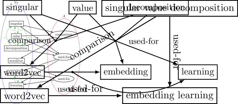
(c) Incidence graph with $\textsc{same}{}_{p}$ edges (dashed green)

Figure 1: Different representations of the same KG (types are omitted for clarity).

3.1 Graph data structure

Knowledge graph. We formalize a knowledge graph (KG) as a directed, labeled multigraph $G_{\mathit{KG}}=\left(V,A,s,t,l_{V},l_{A},\mathcal{E},\mathcal{R}\right)$ with $V$ a set of vertices (the KG entities), $A$ a set of arcs (the KG facts), $s,t:A\to V$ functions assigning to each arc its source/target node (the subject/object of a KG fact), and $l_{V}:V\to\mathcal{E},l_{A}:A\to\mathcal{R}$ providing labels for vertices and arcs, where $\mathcal{R}$ is a set of KG-specific relations and $\mathcal{E}$ a set of entity names.

Token graph. Entity names usually consist of more than one token or subword unit. Hence, a tokenizer $\mathit{tok}:\mathcal{E}\to\Sigma_{T}^{*}$ is needed that splits an entity’s label into its components from the vocabulary $\Sigma_{T}$ of text tokens. Following recent work (Ribeiro et al., 2020), we mimic this compositionality of node labels in the graph structure by splitting each node into as many nodes as there are tokens in its label. We thus obtain a directed hypergraph $G_{T}=\left(V_{T},A,s_{T},t_{T},l_{T},l_{A},\Sigma_{T},\mathcal{R},\mathit{same}{}\right)$, where $s_{T},t_{T}:A\to\mathcal{P}\left(V_{T}\right)$ now assign a set of source (resp. target) nodes to each (hyper-) arc and all nodes are labeled with only one token, i.e., $l_{T}:V_{T}\to\Sigma_{T}$. Unlike Ribeiro et al. (2020), we additionally keep track of all token nodes’ origins: $\mathit{same}{}:V_{T}\to\mathcal{P}\left(V_{T}\times\mathbb{Z}\right)$ assigns to each node $n$ all other nodes $n^{\prime}$ stemming from the same entity together with the relative position of $l_{T}(n)$ and $l_{T}(n^{\prime})$ in the original tokenized entity name. Fig. 1(b) shows the token graph corresponding to the KG in Fig. 1(a).

Incidence graph. For ease of implementation, our final data structure for the KG is the hypergraph’s incidence graph, a bipartite graph where hyper-arcs are represented as nodes and edges are unlabeled: $G=\left(N,E,l,\Sigma,\left\{\,\textsc{same}{}_{p}\mid p\in\mathbb{Z}\,\right\}\right)$ where $N=V_{T}\cup A$ is the set of nodes, $E=\left\{\,\left(n_{1},n_{2}\right)\mid n_{1}\in s_{T}(n_{2})\lor n_{2}\in t_{T}(n_{1})\,\right\}$ the set of directed edges, $l:N\to\Sigma$ a label function, and $\Sigma=\Sigma_{T}\cup\mathcal{R}$ the vocabulary. We introduce $\textsc{same}{}_{p}$ edges to fully connect $\mathit{same}$ clusters: $\textsc{same}{}_{p}=\left\{\,\left(n_{1},n_{2}\right)\mid\left(n_{2},p\right)\in\mathit{same}{}(n_{1})\,\right\}$ where $p$ differentiates between different relative positions in the original entity string, similar to (Shaw et al., 2018). See Fig. 1(c) for an example.

3.2 Graformer encoder

The initial graph representation $\bm{H}^{(0)}\in\mathbb{R}^{\left|N\right|\times d}$ is obtained by looking up embeddings for the node labels in the learned embedding matrix $\bm{E}\in\mathbb{R}^{\left|\Sigma\right|\times d}$, i.e., $\bm{H}_{i}^{(0)}=\bm{e}^{l(n_{i})}\bm{E}$ where $\bm{e}^{l(n_{i})}$ is the one-hot-encoding of the $i$th node’s label.

To compute the node representation $\bm{H}^{(L)}$ in the $L$th layer, we follow Vaswani et al. (2017), i.e., we first normalize the input from the previous layer $\bm{H}^{(L-1)}$ via layer normalization $\mathit{LN}$, followed by multi-head graph self-attention $\mathit{SelfAtt}_{g}$ (see § 3.3 for details), which – after dropout regularization $\mathit{Dr}$ and a residual connection – yields the intermediate representation $\bm{\mathcal{I}}$ (cf. Eq. 1). A feedforward layer $\mathit{FF}$ with one hidden layer and GeLU (Hendrycks and Gimpel, 2016) activation computes the final layer output (cf. Eq. 2). As recommended by Chen et al. (2018), we apply an additional layer normalization step to the output $\bm{H}^{(L_{E})}$ of the last encoder layer $L_{E}$.

$$\bm{\mathcal{I}}^{(L)} =\mathit{Dr}(\mathit{SelfAtt}_{g}(\mathit{LN}(\bm{H}^{(L-1)})))+\bm{H}^{(L-1)}$$ (1)

$$\bm{H}^{(L)} =\mathit{Dr}(\mathit{FF}(\mathit{LN}(\bm{\mathcal{I}}^{(L)})))+\bm{\mathcal{I}}^{(L)}$$ (2)

$\mathit{SelfAtt}_{g}$ computes a weighted sum of $\bm{H}^{(L-1)}$:

$$\mathit{SelfAtt}_{g}(\bm{H})_{i}=\sum_{j=1}^{\left|N\right|}\alpha_{ij}^{g}(\bm{H}_{j}\bm{W}^{V_{g}})$$ (3)

where $\bm{W}^{V_{g}}\in\mathbb{R}^{d\times d}$ is a learned parameter matrix.

In the next section, we derive the definition of the graph-structure-informed attention weights $\alpha_{ij}^{g}$.

3.3 Self-attention for text and graphs with relative position embeddings

In this section, we describe the computation of attention weights for multi-head self-attention. Note that the formulas describe the computations for one head. The output of multiple heads is combined as in the original Transformer (Vaswani et al., 2017).

Text self-attention. Shaw et al. (2018) introduced position-aware self-attention in the Transformer by (i) adding a relative position embedding $\bm{\mathsfit{A}}^{K}\in\mathbb{R}^{M\times M\times d}$ to $\bm{X}$’s key representation, when computing the softmax-normalized attention scores $\bm{\alpha}_{i}$ between $\bm{X}_{i}\in\mathbb{R}^{d}$ and the complete input embedding matrix $\bm{X}\in\mathbb{R}^{M\times d}$ (cf. Eq. 4), and (ii) adding a second type of position embedding $\bm{\mathsfit{A}}^{V}\in\mathbb{R}^{M\times M\times d}$ to $\bm{X}$’s value representation when computing the weighted sum (cf. Eq. 5):

$$\bm{\alpha}_{i} =\sigma\left(\frac{\bm{X}_{i}\bm{W}^{Q}(\bm{X}\bm{W}^{K}+\bm{\mathsfit{A}}^{K}_{i})^{\top}}{\sqrt{d}}\right)$$ (4)

$$\bm{V}_{i} =\sum_{j=1}^{n}\alpha_{ij}(\bm{X}_{j}\bm{W}^{V}+\bm{\mathsfit{A}}_{ij}^{V})$$ (5)

where $\sigma\left(\cdot\right)$ denotes the softmax function, i.e.,

$$\sigma\left(\bm{b}\right)_{i}=\frac{\exp\left(b_{i}\right)}{\sum_{j=1}^{J}\exp\left(b_{j}\right)},\quad\text{for $\bm{b}\in\mathbb{R}^{J}$.}$$

Recent work (Raffel et al., 2019) has adopted a simplified form where value-modifying embeddings $\bm{\mathsfit{A}}^{V}$ are omitted and key-modifying embeddings $\bm{\mathsfit{A}}^{K}$ are replaced with learned scalar embeddings $\bm{S}\in\mathbb{R}^{M\times M}$ that – based on relative position – directly in- or decrease attention scores before normalization, i.e., Eq. 4 becomes Eq. 6.

$$\bm{\alpha}_{i}=\sigma\left(\frac{\bm{X}_{i}\bm{W}^{Q}(\bm{X}\bm{W}^{K})^{\top}}{\sqrt{d}}+\bm{S}_{i}\right)$$ (6)

Shaw et al. (2018) share their position embeddings across attention heads but learn separate embeddings for each layer as word representations from different layers can vary a lot. Raffel et al. (2019) learn separate $\bm{S}$ matrices for each attention head but share them across layers. We use Raffel et al. (2019)’s form of relative position encoding for text self-attention in our decoder (§ 3.4).

	$V_{T}$						$A$
	s	v	d	w	e	l	c	u1	u2
s	0	4	5	2	2	2	1	1	3
v	-4	0	4	2	2	2	1	1	3
d	-5	-4	0	2	2	2	1	1	3
w	-2	-2	-2	0	2	2	-1	$\infty$	1
e	-2	-2	-2	-2	0	4	-3	-1	-1
l	-2	-2	-2	-2	-4	0	-3	-1	-1
c	-1	-1	-1	1	3	3	0	$\infty$	2
u1	-1	-1	-1	$\infty$	1	1	$\infty$	0	$\infty$
u2	-3	-3	-3	-1	1	1	-2	$\infty$	0

Figure 2: $\bm{R}$ matrix for the graph in Fig. 1(c) ($\delta_{\mathit{max}}=3$).

Graph self-attention. Analogously to self-attention on text, we define our structural graph self-attention as follows:

$$\bm{\alpha}_{i}^{g}=\sigma\left(\frac{\bm{H}_{i}\bm{W}^{Q_{g}}(\bm{H}\bm{W}^{K_{g}})^{\top}}{\sqrt{d}}+\gamma(\bm{R})_{i}\right)$$ (7)

$\bm{W}^{K_{g}},\bm{W}^{Q_{g}}\in\mathbb{R}^{d\times d}$ are learned matrices and $\gamma:\mathbb{Z}\cup\left\{\infty\right\}\to\mathbb{R}$ looks up learned scalar embeddings for the relative graph positions in $\bm{R}\in\mathbb{R}^{N\times N}$.

We define the relative graph position $R_{ij}$ between the nodes $n_{i}$ and $n_{j}$ with respect to two factors: (i) the text relative position $p$ in the original entity name if $n_{i}$ and $n_{j}$ stem from the same original entity, i.e., $\left(n_{i},n_{j}\right)\in\textsc{same}{}_{p}$ for some $p$ and (ii) shortest path lengths otherwise:

$$R_{ij}=\begin{cases}\infty,&\text{if }\delta(n_{i},n_{j})=\infty\\ &\text{and }\delta(n_{j},n_{i})=\infty\\ \mathit{encode}(p),&\text{if }\left(n_{i},n_{j}\right)\in\textsc{same}{}_{p}\\ \delta(n_{i},n_{j}),&\text{if }\delta(n_{i},n_{j})\leq\delta(n_{j},n_{i})\\ -\delta(n_{j},n_{i}),&\text{if }\delta(n_{i},n_{j})>\delta(n_{j},n_{i})\end{cases}$$ (8)

where $\delta(n_{i},n_{j})$ is the length of the shortest path from $n_{i}$ to $n_{j}$, which we define to be $\infty$ if and only if there is no such path. $\mathit{encode}$ maps a text relative position $p\in\mathbb{Z}\setminus\left\{0\right\}$ to an integer outside $\delta$’s range to avoid clashes. Concretely, we use $\mathit{encode}(p):=\mathit{sgn}(p)\cdot\delta_{\mathit{max}}+p$ where $\delta_{\mathit{max}}$ is the maximum graph diameter, i.e., the maximum value of $\delta$ over all graphs under consideration.

Thus, we model graph relative position as the length of the shortest path using either only forward edges ($R_{ij}>0$) or only backward edges ($R_{ij}<0$). Additionally, two special cases are considered: (i) Nodes without any purely forward or purely backward path between them ($R_{ij}=\infty$) and (ii) token nodes from the same entity. Here the relative position in the original entity string $p$ is encoded outside the range of path length encodings (which are always in the interval $\interval{-\delta_{\mathit{max}}}{\delta_{\mathit{max}}}$).

In practice, we use two thresholds, $n_{\delta}$ and $n_{p}$. All values of $\delta$ exceeding $n_{\delta}$ are set to $n_{\delta}$ and analogously for $p$. This limits the number of different positions a model can distinguish.

Intuition. Our definition of relative position in graphs combines several advantages: (i) Any node can attend to any other node – even unreachable ones – while learning a suitable attention bias for different distances. (ii) $\textsc{same}{}_{p}$edges are treated differently in the attention mechanism. Thus, entity representations can be learned like in a regular transformer encoder, given that tokens from the same entity are fully connected with $\textsc{same}{}_{p}$ edges with $p$ providing relative position information. (iii) The lengths of shortest paths often have an intuitively useful interpretation in our incidence graphs and the sign of the entries in $\bm{R}$ also captures the important distinction between incoming and outgoing paths. In this way, Graformer can, e.g., capture the difference between the subject and object of a fact, which is expressed as a relative position of $-1$ vs. $1$. The subject and object nodes, in turn, see each other as $2$ and $-2$, respectively.

Fig. 2 shows the $\bm{R}$ matrix corresponding to the graph from Fig. 1(c). Note how token nodes from the same entity, e.g., s, v, and d, form clusters as they have the same distances to other nodes, and how the relations inside such a cluster are encoded outside the interval $\interval{-3}{3}$, i.e., the range of shortest path lengths. It is also insightful to compare node pairs with the same value in $\bm{R}$. E.g., both s and w see e at a distance of $2$ because the entities SVD and word2vec are both the subject of a fact with embedding learning as the object. Likewise, s sees both c and u1 at a distance of $1$ because its entity SVD is subject to both corresponding facts.

3.4 Graformer decoder

Our decoder follows closely the standard Transformer decoder (Vaswani et al., 2017), except for the modifications suggested by Chen et al. (2018).

Hidden decoder representation. The initial decoder representation $\bm{Z}^{(0)}\in\mathbb{R}^{M\times d}$ embeds the (partially generated) target text $\bm{T}\in\mathbb{R}^{M\times\left|\Sigma\right|}$, i.e., $\bm{Z}^{(0)}=\bm{T}\bm{E}$. A decoder layer $L$ then obtains a contextualized representation via self-attention as in the encoder (§ 3.2):

$$\bm{C}^{(L)}=\mathit{Dr}(\mathit{SelfAtt}_{t}(\mathit{LN}(\bm{Z}^{(L-1)})))+\bm{Z}^{(L-1)}$$ (9)

$\mathit{SelfAtt}_{t}$ differs from $\mathit{SelfAtt}_{g}$ by using different position embeddings in Eq. 7 and, obviously, $R_{ij}$ is defined in the usual way for text. $\bm{C}^{(L)}$ is then modified via multi-head attention $\mathit{MHA}$ on the output $\bm{H}^{(L_{E})}$ of the last graph encoder layer $L_{E}$. As in § 3.2, we make use of residual connections, layer normalization $\mathit{LN}$, and dropout $\mathit{Dr}$:

$$\bm{U}^{(L)} =\mathit{Dr}(\mathit{MHA}(\mathit{LN}(\bm{C}^{(L)}),\bm{H}^{(L_{E})}))+\bm{C}^{(L)}$$ (10)

$$\bm{Z}^{(L)} =\mathit{Dr}(\mathit{FF}(\mathit{LN}(\bm{U}^{(L)})))+\bm{U}^{(L)}$$ (11)

where

$$\mathit{MHA}(\bm{C},\bm{H})_{i}=\sum_{j=1}^{\left|N\right|}\alpha_{ij}(\bm{H}_{j}\bm{W}^{V_{t}})$$ (12)

$$\bm{\alpha}_{i}=\sigma\left(\frac{\bm{C}_{i}\bm{W}^{Q_{t}}(\bm{H}\bm{W}^{K_{t}})^{\top}}{\sqrt{d}}\right)$$ (13)

Generation probabilities. The final representation $\bm{Z}^{(L_{D})}$ of the last decoder layer $L_{D}$ is used to compute the probability distribution $\bm{P}_{i}\in\interval{0}{1}^{\left|\Sigma\right|}$ over all words in the vocabulary $\Sigma$ at time step $i$:

$$\bm{P}_{i}=\sigma\left(\bm{Z}_{i}^{(L_{D})}\bm{E}^{\top}\right)$$ (14)

Note that $\bm{E}\in\mathbb{R}^{\left|\Sigma\right|\times d}$ is the same matrix that is also used to embed node labels and text tokens.

3.5 Training

We train Graformer by minimizing the standard negative log-likelihood loss based on the likelihood estimations described in the previous section.

4 Experiments

4.1 Datasets

We evaluate our new architecture on two popular benchmarks for KG-to-text generation, AGENDA (Koncel-Kedziorski et al., 2019) and WebNLG (Gardent et al., 2017). While the latter contains crowd-sourced texts corresponding to subgraphs from various DBPedia categories, the former was automatically created by applying an information extraction tool (Luan et al., 2018) on a corpus of scientific abstracts (Ammar et al., 2018). As this process is noisy, we corrected 7 train instances where an entity name was erroneously split on a special character and, for the same reason, deleted 1 train instance entirely. Otherwise, we use the data as is, including the train/dev/test split.

We list the number of instances per data split, as well as general statistics about the graphs in Table 1. Note that the graphs in WebNLG are human-authored subgraphs of DBpedia while the graphs in AGENDA were automatically extracted. This leads to a higher number of disconnected graph components. Nearly all WebNLG graphs consist of a single component, i.e., are connected graphs, whereas for AGENDA this is practically never the case. We also report statistics that depend on the tokenization (cf. § 4.2) as factors like the length of target texts and the percentage of tokens shared verbatim between input graph and target text largely impact the task difficulty.

	AGENDA	WebNLG
#instances in train	38,719	18,102
#instances in val	1,000	872
#instances in test	1,000	971
#relation types	7	373
avg #entities in KG	13.4	4.0
% connected graphs	0.3	99.9
avg #graph components	8.4	1.0
avg component size	1.6	3.9
avg #token nodes in graph	98.0	36.0
avg #tokens in text	157.9	31.5
avg % text tokens in graph	42.7	56.1
avg % graph tokens in text	48.6	49.0
Vocabulary size $\left|\Sigma\right|$	24,100	2,100
Character coverage in %	99.99	100.0

Table 1: Statistics of AGENDA and the dataset from the WebNLG challenge as used in our experiments. Upper part: data splits and original KGs. Lower part: token graphs and BPE settings.

4.2 Data preprocessing

Following previous work on AGENDA (Ribeiro et al., 2020), we put the paper title into the graph as another entity. In contrast to Ribeiro et al. (2020), we also link every node from a real entity to every node from the title by title2txt and txt2title edges. The type information provided by AGENDA is, as usual for KGs, expressed with one dedicated node per type and has-type arcs that link entities to their types. We keep the original pretokenized texts but lowercase the title as both node labels and target texts are also lowercased.

For WebNLG, we follow previous work (Gardent et al., 2017) by replacing underscores in entity names with whitespace and breaking apart camel-cased relations. We furthermore follow the evaluation protocol of the original challenge by converting all characters to lowercased ASCII and separating all punctuation from alphanumeric characters during tokenization.

For both datasets, we train a BPE vocabulary using sentencepiece (Kudo and Richardson, 2018) on the train set, i.e., a concatenation of node labels and target texts. See Table 1 for vocabulary sizes. Note that for AGENDA, only 99.99% of the characters found in the train set are added to the vocabulary. This excludes exotic Unicode characters that occur in certain abstracts.

We prepend entity and relation labels with dedicated $\langle E\rangle$ and $\langle R\rangle$ tags.

4.3 Hyperparameters and training details

We train Graformer with the Adafactor optimizer (Shazeer and Stern, 2018) for 40 epochs on AGENDA and 200 epochs on WebNLG. We report test results for the model yielding the best validation performance measured in corpus-level BLEU (Papineni et al., 2002). For model selection, we decode greedily. The final results are generated by beam search. Following Ribeiro et al. (2020), we couple beam search with a length penalty (Wu et al., 2016) of $5.0$. See Appendix A for more details and a full list of hyperparameters.

4.4 Epoch curriculum

We apply a data loading scheme inspired by the bucketing approach of Koncel-Kedziorski et al. (2019) and length-based curriculum learning (Platanios et al., 2019): We sort the train set by target text length and split it into four buckets of two times $40\%$ and two times $10\%$ of the data. After each training epoch, the buckets are shuffled internally but their global order stays the same from shorter target texts to longer ones. This reduces padding during batching as texts of similar lengths stay together and introduces a mini-curriculum from presumably easier examples (i.e., shorter targets) to more difficult ones for each epoch. This enables us to successfully train Graformer even without a learning rate schedule.

5 Results and Discussion

5.1 Overall performance

Table 2 shows the results of our evaluation on AGENDA in terms of BLEU (Papineni et al., 2002), METEOR (Banerjee and Lavie, 2005), and CHRF++ (Popović, 2017). Like the models we compare with, we report the average and standard deviation of 4 runs with different random seeds.

Our model outperforms previous Transformer-based models that only consider first-order neighborhoods per encoder layer (Koncel-Kedziorski et al., 2019; An et al., 2019). Compared to the very recent models by Ribeiro et al. (2020), Graformer performs very similarly. Using both a local and a global graph encoder, Ribeiro et al. (2020) combine information from very distant nodes but at the same time need extra parameters for the second encoder. Graformer is more efficient and still matches their best model’s BLEU and METEOR scores within a standard deviation.

The results on the test set of seen categories of WebNLG (Table 3) look similar. Graformer outperforms most original challenge participants and more recent work. While not performing on par with CGE-LW on WebNLG, Graformer still achieves more than 96% of its performance while using only about half as many parameters.

	BLEU	METEOR	CHRF++	#P
Ours	$17.80$ $\pm 0.31$	$22.07$ $\pm 0.23$	$45.43$ $\pm 0.39$	36.3
GT	$14.30$ $\pm 1.01$	$18.80$ $\pm 0.28$	–	–
GT+RBS	$15.1$ $\pm 0.97$	$19.5$ $\pm 0.29$	–	–
CGE-LW	$18.01$ $\pm 0.14$	$22.34$ $\pm 0.07$	$46.69$ $\pm 0.17$	69.8

Table 2: Experimental results on AGENDA. GT (Graph Transformer) from (Koncel-Kedziorski et al., 2019); GT+RBS from (An et al., 2019); CGE-LW from (Ribeiro et al., 2020). Number of parameters in millions.

	BLEU	METEOR	CHRF++	#P
Ours	$61.15$ $\pm 0.22$	$43.38$ $\pm 0.17$	$75.43$ $\pm 0.19$	5.3
UPF-FORGe	40.88	40.00	–	–
Melbourne	54.52	41.00	70.72	–
Adapt	60.59	44.00	76.01	–
Graph Conv.	55.90	39.00	–	4.9
GTR-LSTM	58.60	40.60	–	–
E2E GRU	57.20	41.00	–	–
CGE-LW-LG	$63.69$ $\pm 0.10$	$44.47$ $\pm 0.12$	$76.66$ $\pm 0.10$	10.4

Table 3: Experimental results on the WebNLG test set with seen categories. CGE-LW-LG from (Ribeiro et al., 2020); Adapt, Melbourne and UPF-FORGe from (Gardent et al., 2017); Graph Conv. from (Marcheggiani and Perez-Beltrachini, 2018); GTR-LSTM from (Trisedya et al., 2018); E2E GRU from (Castro Ferreira et al., 2019). Number of parameters in millions.

$\mu_{c}$		BLEU	METEOR	CHRF++
${}<1.25$	Ours	15.44	20.59	43.23
(213)	CGE-LW	15.34	20.64	43.56
${}<1.5$	Ours	17.45	22.03	45.67
(338)	CGE-LW	17.29	22.32	45.88
${}<2.0$	Ours	18.94	22.86	46.49
(294)	CGE-LW	19.46	23.76	47.78
${}\geq 2.0$	Ours	21.72	24.22	48.79
(155)	CGE-LW	20.97	24.98	49.83

(a) Average size $\mu_{c}$ of graph components.

$\mathsf{d}$		BLEU	METEOR	CHRF++
1	Ours	16.48	21.16	43.94
(368)	CGE-LW	16.33	21.16	44.16
2	Ours	18.46	22.70	46.85
(414)	CGE-LW	18.20	23.14	47.28
${}\geq 3$	Ours	19.44	23.17	47.29
(218)	CGE-LW	20.32	24.42	49.25

(b) Largest diameter $\mathsf{d}$ across all of a graph’s components.

Table 4: Performance of a single run on the test split of AGENDA w.r.t. different input graph properties. The number of data points in each split is indicated in parentheses.

(a) AGENDA

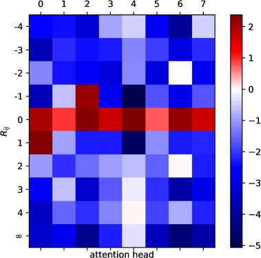
(b) WebNLG

Figure 3: Attention bias $\gamma$ learned by Graformer on the two datasets. $\textsc{same}{}_{p}$ edges are omitted.

5.2 Performance on different types of graphs

We investigate whether Graformer is more suitable for disconnected graphs by comparing its performance on different splits of the AGENDA test set according to two graph properties: (i) the average number of nodes per connected component ($\mu_{c}$) and (ii) the largest diameter across all of a graph’s components ($\mathsf{d}$).

We can see in Table 4 that the performance of both Graformer and CGE-LW (Ribeiro et al., 2020) increases with more graph structure (larger $\mu_{c}$ and $\mathsf{d}$), i.e., more information leads to more accurate texts. Besides, Graformer outperforms CGE-LW on BLEU for graphs with smaller components ($0<\mu_{c}<1.5$) and smaller diameters ($\mathsf{d}\!<\!3$). Although METEOR and CHRF++ scores always favor CGE-LW, the performance difference is also smaller for cases where BLEU favors Graformer.

We conjecture that Graformer benefits from its more elaborate global view, i.e., its ability to distinguish between distant but connected nodes and unreachable ones. CGE-LW’s global encoder cannot make this distinction because it only sees a fully connected version of the graph.

Curiously, Graformer’s BLEU is also better for larger components ($\mu_{c}\geq 2.0$). With multiple larger components, Graformer might also better distinguish nodes that are part of the same component from those that belong to a different one.

Only for $1.5<\mu_{c}<2.0$, CGE-LW clearly outperforms Graformer in all metrics. It seems that Graformer is most helpful for extreme cases, i.e., when either most components are isolated nodes or when isolated nodes are the exception.

Model	BLEU	METEOR	CHRF++
Graformer	18.09	22.29	45.77
-length penalty	17.99	22.19	45.63
-beam search	17.33	21.74	44.87
-epoch curriculum	13.55	18.91	39.22

Table 5: Ablation study for a single run on the test portion of AGENDA.

5.3 Ablation study

In a small ablation study, we examine the impact of beam search, length penalty, and our new epoch curriculum training. We find that beam search and length penalty do contribute to the overall performance but to a relatively small extent. Training with our new epoch curriculum, however, proves crucial for good performance. Platanios et al. (2019) argue that curriculum learning can replace a learning rate schedule, which is usually essential to train a Transformer model. Indeed we successfully optimize Graformer without any learning rate schedule, when applying the epoch curriculum.

6 Learned graph structure

We visualize the learned attention bias $\gamma$ for different relative graph positions $R_{ij}$ (cf. § 3.3; esp. Eq. 7) after training on AGENDA and WebNLG in Fig. 3. The eight attention heads (x-axis) have learned different weights for each graph position $R_{ij}$ (y-axis). Note that AGENDA has more possible $R_{ij}$ values because $n_{\delta}=6$ whereas we set $n_{\delta}=4$ for WebNLG.

For both datasets, we notice that one attention head primarily focuses on global information (5 for AGENDA, 4 for WebNLG). AGENDA even dedicates head 6 entirely to unreachable nodes, showing the importance of such nodes for this dataset. In contrast, most WebNLG heads suppress information from unreachable nodes.

For both datasets, we also observe that nearer nodes generally receive a high weight (focus on local information): In Fig. 3(b), e.g., head 2 concentrates solely on direct incoming edges and head 0 on direct outgoing ones. Graformer can learn empirically based on its task where direct neighbors are most important and where they are not, showing that the strong bias from graph neural networks is not necessary to learn about graph structure.

7 Conclusion

We presented Graformer, a novel encoder-decoder architecture for graph-to-text generation based on Transformer. The Graformer encoder uses a novel type of self-attention for graphs based on shortest path lengths between nodes, allowing it to detect global patterns by automatically learning appropriate weights for higher-order neighborhoods. In our experiments on two popular benchmarks for text generation from knowledge graphs, Graformer achieved competitive results while using many fewer parameters than alternative models.

Appendix A Hyperparameter details

For AGENDA and WebNLG, a minimum and maximum decoding length were set according to the shortest and longest target text in the train set. Table 6 lists the hyperparameters used to obtain final results on both datasets. Input dropout is applied on the word embeddings directly after lookup for node labels and target text tokens before they are fed into encoder or decoder. Attention dropout is applied to all attention weights computed during multi-head (self-)attention.

For hyperparameter optimization, we only train for the first 10 (AGENDA) or 50 (WebNLG) epochs to save time. We use a combination of manual tuning and a limited number of randomly sampled runs. For the latter we apply Optuna with default parameters (Akiba et al., 2019; Bergstra et al., 2011) and median pruning, i.e., after each epoch of a particular hyperparameter run we check if the best performance so far is worse than the median performance of previous runs at the same epoch and if so, abort. For hyperparameter tuning, we decode greedily and measure performance in corpus-level BLEU (Papineni et al., 2002).

Hyperparameter	WebNLG	AGENDA
model dimension $d$	256	400
# heads	8	8
# encoder layers $L_{E}$	3	4
# decoder layers $L_{D}$	3	5
feedforward dimension	512	2000
attention dropout	0.3	0.1
dropout	0.1	0.1
input dropout	0.0	0.1
text self-attention range $n_{t}$	25	50
graph self-attention range $n_{\delta}$	4	6
same range $n_{p}$	10	10
gradient accumulation	3	2
gradient clipping	1.0	1.0
label smoothing	0.25	0.3
$L_{2}$ regularizer	$3\cdot 10^{-3}$	$3\cdot 10^{-4}$
batch size	4	8
# beams	2	2
length penalty	5.0	5.0

Table 6: Hyperparameters used to obtain final experimental results on WebNLG and AGENDA.

Appendix B Qualitative examples

Table 7 shows three example generations from our Graformer model and the CGE-LW system by Ribeiro et al. (2020). Often CGE-LW generations have a high surface overlap with the reference text while Graformer texts fluently express the same content.

Ref.	julia morgan has designed many significant buildings , including the los angeles herald examiner building .
CGE-LW	julia morgan has designed many significant buildings including the los angeles herald examiner building .
Ours	one of the significant buildings designed by julia morgan is the los angeles herald examiner building .
Ref.	asam pedas is a dish of fish cooked in a sour and hot sauce that comes from indonesia .
CGE-LW	the main ingredients of asam pedas are fish cooked in a sour and hot sauce and comes from indonesia .
Ours	the main ingredients of asam pedas are fish cooked in sour and hot sauce . the dish comes from indonesia .
Ref.	banana is an ingredient in binignit which is a dessert . a cookie is also a dessert .
CGE-LW	banana is an ingredient in binignit , a cookie is also a dessert .
Ours	a cookie is a dessert , as is binignit , which contains banana as one of its ingredients .

Table 7: Example references and texts generated by CGE-LW (Ribeiro et al., 2020) and Graformer (marked Ours) for samples from the WebNLG test set. In case of multiple references, only one is shown for brevity.

References

- Akiba et al. (2019) Takuya Akiba, Shotaro Sano, Toshihiko Yanase, Takeru Ohta, and Masanori Koyama. 2019. Optuna: A next-generation hyperparameter optimization framework. In Proceedings of the 25rd ACM SIGKDD International Conference on Knowledge Discovery and Data Mining.
- Ammar et al. (2018) Waleed Ammar, Dirk Groeneveld, Chandra Bhagavatula, Iz Beltagy, Miles Crawford, Doug Downey, Jason Dunkelberger, Ahmed Elgohary, Sergey Feldman, Vu Ha, Rodney Kinney, Sebastian Kohlmeier, Kyle Lo, Tyler Murray, Hsu-Han Ooi, Matthew Peters, Joanna Power, Sam Skjonsberg, Lucy Wang, Chris Wilhelm, Zheng Yuan, Madeleine van Zuylen, and Oren Etzioni. 2018. Construction of the literature graph in semantic scholar. In Proceedings of the 2018 Conference of the North American Chapter of the Association for Computational Linguistics: Human Language Technologies, Volume 3 (Industry Papers), pages 84–91, New Orleans - Louisiana. Association for Computational Linguistics.
- An et al. (2019) Bang An, Xuannan Dong, and Changyou Chen. 2019. Repulsive bayesian sampling for diversified attention modeling. 4th workshop on Bayesian Deep Learning (NeurIPS 2019).
- Auer et al. (2008) Sören Auer, Chris Bizer, Georgi Kobilarov, Jens Lehmann, Richard Cyganiak, and Zachary Ives. 2008. DBpedia: A nucleus for a web of open data. In Proceedings of the 6th International Semantic Web Conference (ISWC), volume 4825 of Lecture Notes in Computer Science, pages 722–735. Springer.
- Banerjee and Lavie (2005) Satanjeev Banerjee and Alon Lavie. 2005. METEOR: An automatic metric for MT evaluation with improved correlation with human judgments. In Proceedings of the ACL Workshop on Intrinsic and Extrinsic Evaluation Measures for Machine Translation and/or Summarization, pages 65–72, Ann Arbor, Michigan. Association for Computational Linguistics.
- Bergstra et al. (2011) James S. Bergstra, Rémi Bardenet, Yoshua Bengio, and Balázs Kégl. 2011. Algorithms for hyper-parameter optimization. In J. Shawe-Taylor, R. S. Zemel, P. L. Bartlett, F. Pereira, and K. Q. Weinberger, editors, Advances in Neural Information Processing Systems 24, pages 2546–2554. Curran Associates, Inc.
- Bhowmik and de Melo (2018) Rajarshi Bhowmik and Gerard de Melo. 2018. Generating fine-grained open vocabulary entity type descriptions. In Proceedings of the 56th Annual Meeting of the Association for Computational Linguistics (Volume 1: Long Papers), pages 877–888, Melbourne, Australia. Association for Computational Linguistics.
- Cai and Lam (2020) Deng Cai and Wai Lam. 2020. Graph transformer for graph-to-sequence learning. AAAI Conference on Artificial Intelligence.
- Castro Ferreira et al. (2019) Thiago Castro Ferreira, Chris van der Lee, Emiel van Miltenburg, and Emiel Krahmer. 2019. Neural data-to-text generation: A comparison between pipeline and end-to-end architectures. In Proceedings of the 2019 Conference on Empirical Methods in Natural Language Processing and the 9th International Joint Conference on Natural Language Processing (EMNLP-IJCNLP), pages 552–562, Hong Kong, China. Association for Computational Linguistics.
- Chen et al. (2018) Mia Xu Chen, Orhan Firat, Ankur Bapna, Melvin Johnson, Wolfgang Macherey, George Foster, Llion Jones, Mike Schuster, Noam Shazeer, Niki Parmar, Ashish Vaswani, Jakob Uszkoreit, Lukasz Kaiser, Zhifeng Chen, Yonghui Wu, and Macduff Hughes. 2018. The best of both worlds: Combining recent advances in neural machine translation. In Proceedings of the 56th Annual Meeting of the Association for Computational Linguistics (Volume 1: Long Papers), pages 76–86, Melbourne, Australia. Association for Computational Linguistics.
- Gardent et al. (2017) Claire Gardent, Anastasia Shimorina, Shashi Narayan, and Laura Perez-Beltrachini. 2017. The WebNLG challenge: Generating text from RDF data. In Proceedings of the 10th International Conference on Natural Language Generation, pages 124–133, Santiago de Compostela, Spain. Association for Computational Linguistics.
- Guo et al. (2019) Zhijiang Guo, Yan Zhang, Zhiyang Teng, and Wei Lu. 2019. Densely connected graph convolutional networks for graph-to-sequence learning. Transactions of the Association for Computational Linguistics, 7:297–312.
- Hendrycks and Gimpel (2016) Dan Hendrycks and Kevin Gimpel. 2016. Gaussian error linear units (gelus). Computing Research Repository, arXiv:1606.08415.
- Hochreiter and Schmidhuber (1997) Sepp Hochreiter and Jürgen Schmidhuber. 1997. Long short-term memory. Neural computation, 9:1735–80.
- Kipf and Welling (2017) Thomas N. Kipf and Max Welling. 2017. Semi-supervised classification with graph convolutional networks. In International Conference on Learning Representations (ICLR).
- Koncel-Kedziorski et al. (2019) Rik Koncel-Kedziorski, Dhanush Bekal, Yi Luan, Mirella Lapata, and Hannaneh Hajishirzi. 2019. Text Generation from Knowledge Graphs with Graph Transformers. In Proceedings of the 2019 Conference of the North American Chapter of the Association for Computational Linguistics: Human Language Technologies, Volume 1 (Long and Short Papers), pages 2284–2293, Minneapolis, Minnesota. Association for Computational Linguistics.
- Krishna et al. (2017) Ranjay Krishna, Yuke Zhu, Oliver Groth, Justin Johnson, Kenji Hata, Joshua Kravitz, Stephanie Chen, Yannis Kalantidis, Li-Jia Li, David A. Shamma, Michael S. Bernstein, and Fei-Fei Li. 2017. Visual genome: Connecting language and vision using crowdsourced dense image annotations. International Journal of Computer Vision, 123:32–73.
- Kudo and Richardson (2018) Taku Kudo and John Richardson. 2018. SentencePiece: A simple and language independent subword tokenizer and detokenizer for neural text processing. In Proceedings of the 2018 Conference on Empirical Methods in Natural Language Processing: System Demonstrations, pages 66–71, Brussels, Belgium. Association for Computational Linguistics.
- Li et al. (2018) Qimai Li, Zhichao Han, and Xiao ming Wu. 2018. Deeper insights into graph convolutional networks for semi-supervised learning. AAAI Conference on Artificial Intelligence.
- Luan et al. (2018) Yi Luan, Luheng He, Mari Ostendorf, and Hannaneh Hajishirzi. 2018. Multi-task identification of entities, relations, and coreference for scientific knowledge graph construction. In Proceedings of the 2018 Conference on Empirical Methods in Natural Language Processing, pages 3219–3232, Brussels, Belgium. Association for Computational Linguistics.
- Marcheggiani and Perez-Beltrachini (2018) Diego Marcheggiani and Laura Perez-Beltrachini. 2018. Deep graph convolutional encoders for structured data to text generation. In Proceedings of the 11th International Conference on Natural Language Generation, pages 1–9, Tilburg University, The Netherlands. Association for Computational Linguistics.
- Moryossef et al. (2019) Amit Moryossef, Yoav Goldberg, and Ido Dagan. 2019. Step-by-step: Separating planning from realization in neural data-to-text generation. In Proceedings of the 2019 Conference of the North American Chapter of the Association for Computational Linguistics: Human Language Technologies, Volume 1 (Long and Short Papers), pages 2267–2277, Minneapolis, Minnesota. Association for Computational Linguistics.
- Papineni et al. (2002) Kishore Papineni, Salim Roukos, Todd Ward, and Wei-Jing Zhu. 2002. Bleu: a method for automatic evaluation of machine translation. In Proceedings of the 40th Annual Meeting of the Association for Computational Linguistics, pages 311–318, Philadelphia, Pennsylvania, USA. Association for Computational Linguistics.
- Pei et al. (2020) Hongbin Pei, Bingzhe Wei, Kevin Chen-Chuan Chang, Yu Lei, and Bo Yang. 2020. Geom-gcn: Geometric graph convolutional networks. In International Conference on Learning Representations (ICLR).
- Platanios et al. (2019) Emmanouil Antonios Platanios, Otilia Stretcu, Graham Neubig, Barnabas Poczos, and Tom Mitchell. 2019. Competence-based curriculum learning for neural machine translation. In Proceedings of the 2019 Conference of the North American Chapter of the Association for Computational Linguistics: Human Language Technologies, Volume 1 (Long and Short Papers), pages 1162–1172, Minneapolis, Minnesota. Association for Computational Linguistics.
- Popović (2017) Maja Popović. 2017. chrF++: words helping character n-grams. In Proceedings of the Second Conference on Machine Translation, pages 612–618, Copenhagen, Denmark. Association for Computational Linguistics.
- Raffel et al. (2019) Colin Raffel, Noam Shazeer, Adam Roberts, Katherine Lee, Sharan Narang, Michael Matena, Yanqi Zhou, Wei Li, and Peter J. Liu. 2019. Exploring the limits of transfer learning with a unified text-to-text transformer. Computing Research Repository, arXiv:1910.10683.
- Ribeiro et al. (2019) Leonardo F. R. Ribeiro, Claire Gardent, and Iryna Gurevych. 2019. Enhancing AMR-to-text generation with dual graph representations. In Proceedings of the 2019 Conference on Empirical Methods in Natural Language Processing and the 9th International Joint Conference on Natural Language Processing (EMNLP-IJCNLP), pages 3183–3194, Hong Kong, China. Association for Computational Linguistics.
- Ribeiro et al. (2020) Leonardo F. R. Ribeiro, Yue Zhang, Claire Gardent, and Iryna Gurevych. 2020. Modeling global and local node contexts for text generation from knowledge graphs. Transactions of the Association for Computational Linguistics, 8(0):589–604.
- Schmitt et al. (2020) Martin Schmitt, Sahand Sharifzadeh, Volker Tresp, and Hinrich Schütze. 2020. An unsupervised joint system for text generation from knowledge graphs and semantic parsing. In Proceedings of the 2020 Conference on Empirical Methods in Natural Language Processing (EMNLP), pages 7117–7130, Online. Association for Computational Linguistics.
- Shaw et al. (2018) Peter Shaw, Jakob Uszkoreit, and Ashish Vaswani. 2018. Self-attention with relative position representations. In Proceedings of the 2018 Conference of the North American Chapter of the Association for Computational Linguistics: Human Language Technologies, Volume 2 (Short Papers), pages 464–468, New Orleans, Louisiana. Association for Computational Linguistics.
- Shazeer and Stern (2018) Noam Shazeer and Mitchell Stern. 2018. Adafactor: Adaptive learning rates with sublinear memory cost. In Proceedings of the 35th International Conference on Machine Learning, volume 80 of Proceedings of Machine Learning Research, pages 4596–4604. PMLR.
- Trisedya et al. (2018) Bayu Distiawan Trisedya, Jianzhong Qi, Rui Zhang, and Wei Wang. 2018. GTR-LSTM: A triple encoder for sentence generation from RDF data. In Proceedings of the 56th Annual Meeting of the Association for Computational Linguistics (Volume 1: Long Papers), pages 1627–1637, Melbourne, Australia. Association for Computational Linguistics.
- Vaswani et al. (2017) Ashish Vaswani, Noam Shazeer, Niki Parmar, Jakob Uszkoreit, Llion Jones, Aidan N Gomez, Łukasz Kaiser, and Illia Polosukhin. 2017. Attention is all you need. In I. Guyon, U. V. Luxburg, S. Bengio, H. Wallach, R. Fergus, S. Vishwanathan, and R. Garnett, editors, Advances in Neural Information Processing Systems 30, page 5998–6008. Curran Associates, Inc.
- Veličković et al. (2018) Petar Veličković, Guillem Cucurull, Arantxa Casanova, Adriana Romero, Pietro Liò, and Yoshua Bengio. 2018. Graph Attention Networks. In International Conference on Learning Representations (ICLR).
- Wishart et al. (2018) David S Wishart, Yannick D Feunang, An C Guo, Elvis J Lo, Ana Marcu, Jason R Grant, Tanvir Sajed, Daniel Johnson, Carin Li, Zinat Sayeeda, Nazanin Assempour, Ithayavani Iynkkaran, Yifeng Liu, Adam Maciejewski, Nicola Gale, Alex Wilson, Lucy Chin, Ryan Cummings, Diana Le, Allison Pon, Craig Knox, and Michael Wilson. 2018. DrugBank 5.0: a major update to the DrugBank database for 2018. Nucleic Acids Research, 46(D1):D1074–D1082.
- Wu et al. (2016) Yonghui Wu, Mike Schuster, Zhifeng Chen, Quoc V. Le, Mohammad Norouzi, Wolfgang Macherey, Maxim Krikun, Yuan Cao, Qin Gao, Klaus Macherey, Jeff Klingner, Apurva Shah, Melvin Johnson, Xiaobing Liu, Łukasz Kaiser, Stephan Gouws, Yoshikiyo Kato, Taku Kudo, Hideto Kazawa, Keith Stevens, George Kurian, Nishant Patil, Wei Wang, Cliff Young, Jason Smith, Jason Riesa, Alex Rudnick, Oriol Vinyals, Greg Corrado, Macduff Hughes, and Jeffrey Dean. 2016. Google’s neural machine translation system: Bridging the gap between human and machine translation. Computing Research Repository, arXiv:1609.08144.
- Zhang et al. (2020) Kai Zhang, Yaokang Zhu, Jun Wang, and Jie Zhang. 2020. Adaptive structural fingerprints for graph attention networks. In International Conference on Learning Representations (ICLR).
- Zhu et al. (2019) Jie Zhu, Junhui Li, Muhua Zhu, Longhua Qian, Min Zhang, and Guodong Zhou. 2019. Modeling graph structure in transformer for better AMR-to-text generation. In Proceedings of the 2019 Conference on Empirical Methods in Natural Language Processing and the 9th International Joint Conference on Natural Language Processing (EMNLP-IJCNLP), pages 5459–5468, Hong Kong, China. Association for Computational Linguistics.