Hessian-Free High-Resolution Nesterov Acceleration For Sampling

Abstract

Nesterov’s Accelerated Gradient (NAG) for optimization has better performance than its continuous time limit (noiseless kinetic Langevin) when a finite step-size is employed (Shi et al., 2021). This work explores the sampling counterpart of this phenonemon and proposes a diffusion process, whose discretizations can yield accelerated gradient-based MCMC methods. More precisely, we reformulate the optimizer of NAG for strongly convex functions (NAG-SC) as a Hessian-Free High-Resolution ODE, change its high-resolution coefficient to a hyperparameter, inject appropriate noise, and discretize the resulting diffusion process. The acceleration effect of the new hyperparameter is quantified and it is not an artificial one created by time-rescaling. Instead, acceleration beyond underdamped Langevin in $W_{2}$ distance is quantitatively established for log-strongly-concave-and-smooth targets, at both the continuous dynamics level and the discrete algorithm level. Empirical experiments in both log-strongly-concave and multi-modal cases also numerically demonstrate this acceleration.

1 Introduction

Optimization is a major machinery that drives the theory and practice of machine learning in recent years. Since the seminal work of Nesterov (1983), acceleration has played a key role in gradient-based optimization methods. A notable example is Nesterov’s Accelerated Gradient (NAG), which is an instance of a more general family of “momentum methods”. NAG consists of multiple methods, including NAG-C and NAG-SC, respectively for convex and strongly convex functions. Both provably converge faster than vanilla gradient descent (GD) in their corresponding setups (Nesterov, 1983, 2013). Newer perspectives of acceleration continue to be revealed, e.g., (Su et al., 2014; Wibisono et al., 2016; Wilson et al., 2021; Hu & Lessard, 2017; Attouch et al., 2018; Shi et al., 2021), many based on the interplay between continuous and discrete times. This work aims at turning NAG-SC into a sampler based on this interplay.

In fact, approaches for sampling statistical distributions, such as gradient-based Markov Chain Monte Carlo (MCMC) methods, are also of great importance in machine learning, for example due to their links to statistical inference and abilities to represent uncertainties lacking in optimization-based methods. Although not entirely the same thing, optimization and sampling are closely related: besides seeing a large class of sampling dynamics as optimization dynamics with additional noise, viewing sampling as optimization in probability space also led to important discoveries (e.g., Jordan et al., 1998; Liu & Wang, 2016; Dalalyan, 2017a; Wibisono, 2018; Zhang et al., 2018; Frogner & Poggio, 2020; Chizat & Bach, 2018; Chen et al., 2018a; Ma et al., 2021; Erdogdu & Hosseinzadeh, 2021). In fact, an unadjusted Euler-Maruyama discretization of overdamped Langevin dynamics (abbreviated as OLD here) is commonly considered as the analog of GD in sampling (although many other discretizations are also possible), and often referred to as Unadjusted Langevin Algorithm (ULA) (Roberts et al., 1996) and/or Langevin Monte Carlo (LMC). The convergence properties of the continuous dynamics of OLD, as well as asymptotic and non-asymptotic analyses of its discretizations have been extensively studied (e.g., Roberts et al., 1996; Villani, 2008; Pavliotis, 2014; Dalalyan, 2017b; Durmus & Moulines, 2016; Dalalyan, 2017a; Durmus et al., 2019; Durmus & Moulines, 2019; Vempala & Wibisono, 2019; Cheng & Bartlett, 2018; Dwivedi et al., 2019; Ma et al., 2019; Chewi et al., 2021; Erdogdu & Hosseinzadeh, 2021).

Meanwhile, the notion of acceleration is less quantified in sampling compared to that in optimization, although attention has been rapidly building up. Along this direction, one line is based on diffusion processes such as underdamped Langevin dynamics (ULD). For example, the convergence and nonasymptotics of discretized ULD have been studied by Cheng et al. (2018); Dalalyan & Riou-Durand (2020); Ma et al. (2021), and were demonstrated provably faster than discretized OLD in suitable setups. These are not only great progresses but also forming perspectives complementary to the extensive studies of the convergence of continuous ULD in the mathematical community (e.g, Mattingly et al., 2002; Cao et al., 2019; Dolbeault et al., 2009, 2015; Villani, 2009; Eckmann & Hairer, 2003; Baudoin, 2017; Eberle et al., 2019). Another important line of research is related to accelerating particle-based approaches for optimization in probability spaces (Liu et al., 2019; Taghvaei & Mehta, 2019; Wang & Li, 2019), although we note there is no clear boundary between these two lines (e.g., Leimkuhler et al., 2018). Additional interesting ideas also include (Chen et al., 2018b; Deng et al., 2020; Ding et al., 2021; Li et al., 2022a; Liang & Chen, 2022). In general, it has been known that adding an irreversible part to the reversible dynamics of OLD accelerates its convergence (e.g., Hwang et al., 2005; Lelievre et al., 2013; Ohzeki & Ichiki, 2015; Rey-Bellet & Spiliopoulos, 2015; Duncan et al., 2016), and this work can be viewed to be under this umbrella. Note, though, the discretization of an accelerated continuous process is also important, and it will also be discussed.

Specifically, we propose a class of accelerated gradient-based MCMC algorithms termed HFHR. It is motivated by a simple question: how to appropriately inject noise to NAG algorithm in discrete time, so that it is turned into an algorithm for momentum-accelerated sampling? Note we don’t add noise to the learning-rate$\to 0$ limit of NAG (this has been studied in Ma et al., 2021), because a finite-step-size discretization of this limiting ODE may not converge as fast as NAG with the same learning rate. However, we will still use continuous dynamics as intermediate steps.

More precisely, our first step is to combine existing tools to prepare a non-asymptotic formulation for the later steps. The goal is to better account for NAG’s behavior when a finite (not infinitesimal) learning rate is used. As pointed out in Shi et al. (2021), a low-resolution limiting ODE (Su et al., 2014), albeit being a milestone leading to important research (e.g, Wibisono et al., 2016), does not fully capture the acceleration enabled by NAG — for example, it can’t distinguish between NAG and another momentum method of heavy ball (Polyak, 1964). A reason is, the low-resolution ODE describes the $h\to 0$ limit of NAG, but in practice NAG uses a finite (nonzero) $h$. High-resolution ODE was thus proposed to include additional $\mathcal{O}(h)$ terms to account for the finite $h$ effect (Shi et al., 2021). The original form of high-resolution ODE involves Hessian of the objective function, which is computationally expensive to evaluate and store for high-dimensional problems, but this is a small obstacle that can be overcome (see e.g., Alvarez et al., 2002; Attouch et al., 2020), and we’ll be able to derive a High-Resolution and Hessian-Free limiting ODE for NAG.

Then we replace the high-resolution term’s coefficient in the HFHR ODE by a hyperparameter $\alpha\geq 0$, and then add noise to the resulting ODE in a specific way, which turns it into an SDE suitable for the sampling purpose. This SDE will be termed as HFHR dynamics.

To obtain an actual algorithm, the HFHR SDE is then discretized. We will see, both theoretically and empirically, that nonzero $\alpha$ can lead to accelerated convergence of the sampling algorithm; this acceleration is not an artificial consequence of time-rescaling, which would not give acceleration after discretization with an appropriate step size. For demonstrating this, we will be primarily working with just a 1st-order discretization, which uses 1 (full-)gradient evaluation per iteration and thus suits particularly well low-to-medium-accuracy downstream applications; comparisons will be mainly against other methods that use 1 gradient per step as well. However, since high-order discretizations can improve statistical accuracy and even the speed of convergence (see e.g., Chen et al., 2015; Li et al., 2019; Shen & Lee, 2019), we will also provide a high-order discretization in Appendix F, which again exhibits acceleration and suits high-accuracy applications.

Our presentation is as follows: After detailing the construction of HFHR, we will analyze its convergence, at both the continuous level (HFHR dynamics) and the discrete level (HFHR algorithm). For precise theoretical results, we will consider the setup of log-strongly-concave target distributions, which are commonly considered in the literature (Kim et al., 2016; Bubeck et al., 2018; Dalalyan, 2017b; Dalalyan & Riou-Durand, 2020; Dwivedi et al., 2019; Shen & Lee, 2019). The additional acceleration of HFHR when compared to ULD in continuous time will be demonstrated explicitly in Thm.5.1. For our discretized HFHR algorithm, a non-asymptotic error bound will be obtained (Thm.5.2), which confirms that the additional acceleration in continuous time carries through to the discrete territory. Finally, numerical experiments are provided, verifying the validity and tightness of our theoretical results, and empirically showing HFHR remains advantageous for the nonconvex and high-dim. problems, e.g., Bayesian Neural Networks.

The main contribution of this article is the idea of turning NAG-SC optimizer into a sampler, and the introduction of a new dynamics that is neither overdamped or underdamped Langevin. Theoretical analyses (e.g., Thm.5.2, Cor.5.4 & Rmk.5.5) and numerical experiments (Sec.6) are provided for quantifying the effectiveness of this idea.

2 Background: Langevin Dynamics

Consider sampling from Gibbs measure $\mu$ whose density is $d\mu=\frac{1}{\int e^{-f(\boldsymbol{y})}d\boldsymbol{y}}e^{-f(\boldsymbol{x})}d\boldsymbol{x}$, where $f\mathrel{\mathop{\mathchar 58\relax}}\mathbb{R}^{d}\mapsto\mathbb{R}$ will be called the potential function. Two diffusion processes popular for sampling (and modeling important physical processes too) are named after Langevin. One is overdamped Langevin dynamics (OLD), and the other is kinetic Langevin dynamics (abbreviated as ULD to comply with a convention of calling it underdamped Langevin). They are respectively given by

$$\mbox{(OLD)}\quad d\boldsymbol{q}_{t}=-\nabla f(\boldsymbol{q}_{t})dt+\sqrt{2}d\boldsymbol{W}_{t}$$

$$\mbox{(ULD)}\quad\begin{cases}d\boldsymbol{q}_{t}=\boldsymbol{p}_{t}dt\\ d\boldsymbol{p}_{t}=-\gamma\boldsymbol{p}_{t}dt-\nabla f(\boldsymbol{q}_{t})dt+\sqrt{2\gamma}d\boldsymbol{B}_{t}\end{cases}$$

where $\boldsymbol{q}_{t},\boldsymbol{p}_{t}\in\mathbb{R}^{d}$, $\boldsymbol{W}_{t},\boldsymbol{B}_{t}$ are i.i.d. Wiener processes in $\mathbb{R}^{d}$, and $\gamma>0$ is a friction coefficient. Under mild conditions (e.g., Pavliotis, 2014), OLD converges to $\mu$ and ULD converges to $d\pi(\boldsymbol{q},\boldsymbol{p})=d\mu(\boldsymbol{q})\nu(\boldsymbol{p})d\boldsymbol{p},\,\text{where }\nu(\boldsymbol{p})=(2\pi)^{-\frac{d}{2}}e^{-\nicefrac{{\|\boldsymbol{p}\|^{2}}}{{2}}}$ , so its $\boldsymbol{q}$ marginal follows $\mu$.

OLD and ULD are closely related. In fact, OLD is the $\gamma\to\infty$ overdamping limit of ULD after time dilation (e.g., Pavliotis, 2014). However, OLD is a reversible Markov process but ULD is irreversible, and thus both their equilibrium and non-equilibrium statistical mechanics are different, although closely related too. We will only focus on the convergence to statistical equilibrium (see e.g., Souza & Tao, 2019 for non-equilibrium aspects).

Many celebrated approaches exist for establishing the exponential convergence (a.k.a. geometric ergodicity) of OLD, including the seminal work of (Roberts et al., 1996), the ones using spectral gap (e.g., Dalalyan, 2017b, Lemma 1), synchronous coupling (Villani, 2008, p33-35; Durmus & Moulines, 2019, Proposition 1), functional inequalities such as Poincaré’s inequality (Pavliotis, 2014, Theorem 4.4) and log Sobolev inequality (Vempala & Wibisono, 2019, Theorem 1). There are also fruitful results for ULD, including the ones leveraging Lyapunov function (Mattingly et al., 2002, Theorem 3.2), hypocoercivity (Villani, 2009; Dolbeault et al., 2009, 2015; Roussel & Stoltz, 2018), coupling (Cheng et al., 2018, Theorem 5; Dalalyan & Riou-Durand, 2020, Theorem 1; Eberle et al., 2019, Theorem 2.3), LSI (Ma et al., 2021, Section 3.1), modified Poincaré’s inequality (Cao et al., 2019, Theorem 1), and spectral analysis (Kozlov, 1989; Eckmann & Hairer, 2003).

The study of asymptotic convergence of discretized OLD dates back to at least the 1990s (Meyn et al., 1994; Roberts et al., 1996). The non-asymptotic analysis of LMC discretization of OLD can be found in (Dalalyan, 2017b) and it shows the discretization achieves $\epsilon$ error, in TV distance, in $\tilde{\mathcal{O}}(\nicefrac{{d}}{{\epsilon^{2}}})$ steps. Subsequent results include $\tilde{\mathcal{O}}(\nicefrac{{d}}{{\epsilon^{2}}})$ in $W_{2}$ (Durmus & Moulines, 2016), $\tilde{\mathcal{O}}(\nicefrac{{d}}{{\epsilon}})$ in KL (Cheng & Bartlett, 2018), $\tilde{\mathcal{O}}(\nicefrac{{d}}{{\epsilon}})$ in $W_{2}$ under additional 3rd-order regularity (Durmus & Moulines, 2019), and $\tilde{\mathcal{O}}(\nicefrac{{\sqrt{d}}}{{\epsilon}})$ in $W_{2}$ under additional 3rd-order regularity (Li et al., 2022b). For discretized ULD, one has $\tilde{\mathcal{O}}(\nicefrac{{\sqrt{d}}}{{\epsilon}})$ iteration complexity in $W_{2}$ (Cheng et al., 2018; Dalalyan & Riou-Durand, 2020) and $\tilde{\mathcal{O}}(\nicefrac{{\sqrt{d}}}{{\sqrt{\epsilon}}})$ in KL (Ma et al., 2021). ULD is still generally conceived to be advantageous over OLD and sometimes understood as its momentum-accelerated version.

3 Notations and Conditions

We will use 2-Wasserstein distance to quantify convergence, i.e. $W_{2}(\mu_{1},\mu_{2})=\left(\inf_{\pi\in\Pi(\mu_{1},\mu_{2})}\mathbb{E}_{(\boldsymbol{X},\boldsymbol{Y})\sim\pi}\mathinner{\!\left\lVert\boldsymbol{X}-\boldsymbol{Y}\right\rVert}^{2}\right)^{\frac{1}{2}}$ where $\Pi(\mu_{1},\mu_{2})$ is the set of all couplings of $\mu_{1}$ and $\mu_{2}$.

Assume WLOG that $\boldsymbol{0}\in\mathop{\rm argmin}_{\boldsymbol{x}\in\mathbb{R}^{d}}f(\boldsymbol{x})$. The following condition will also be frequently used.

Assumption 3.1.

(Standard Strong-Convexity and Smoothness Condition) A function $f\in\mathcal{C}^{1}(\mathbb{R}^{d},\mathbb{R})$ is $m$-stronly-convex and $L$-smooth, if there exist constants $m,L>0$ such that $\forall\boldsymbol{x},\boldsymbol{y}\in\mathbb{R}^{d}$, we have

$$\|\nabla f(\boldsymbol{y})-\nabla f(\boldsymbol{x})\|\leq L\|\boldsymbol{y}-\boldsymbol{x}\|\qquad\mbox{ and }$$

$$f(\boldsymbol{y})\geq f(\boldsymbol{x})+\langle\nabla f(\boldsymbol{x}),\boldsymbol{y}-\boldsymbol{x}\rangle+\frac{m}{2}\|\boldsymbol{y}-\boldsymbol{x}\|^{2}$$

For $f\in\mathcal{C}^{2}$, this is equivalent to $mI\preceq\nabla^{2}f\preceq LI$.

The condition number of $f$ is defined as $\kappa\mathrel{\mathop{\mathchar 58\relax}}=\nicefrac{{L}}{{m}}$.

4 The Construction of HFHR dynamics

HFHR is obtained by formulating NAG-SC as a Hessian free high-resolution ODE, lifting the high-resolution term’s coefficient as a free parameter, and adding appropriate noises.

More precisely, let’s start with NAG-SC algorithm:

$$\boldsymbol{x}_{k+1} =\boldsymbol{y}_{k}-s\nabla f(\boldsymbol{y}_{k})$$ (1)

$$\boldsymbol{y}_{k+1} =\boldsymbol{x}_{k+1}+c(\boldsymbol{x}_{k+1}-\boldsymbol{x}_{k})$$ (2)

where $s$ is the learning rate (also known as step size), and $c=\frac{1-\sqrt{ms}}{1+\sqrt{ms}}$ is a constant based on $s$ and the strong convexity coefficient $m$ of $f$; the method also works for non-strongly-convex $f$ though.

A high-resolution ODE description of Eq.(1) & (2) is obtained in Shi et al. (2021, Section 2)

$$\ddot{\boldsymbol{y}}+\sqrt{s}\left(\frac{2(1-c)}{s(1+c)}+\nabla^{2}f(\boldsymbol{y})\right)\dot{\boldsymbol{y}}+\frac{2}{1+c}\nabla f(\boldsymbol{y})=\boldsymbol{0},$$ (3)

which can better account for the effect of non-infinitesimal $s$ than the $s\to 0$ limit (note $c$ depends on $s$). However, in this original form, Hessian of $f$ is involved, which is expensive to compute and store for high-dimensional problems.

To obtain a Hessian-free high-resolution ODE description of Eq.(1) & (2), we first turn the iteration into a ‘mechanical’ version by introducing position $\boldsymbol{q}_{k}=\boldsymbol{y}_{k}$ and momentum $\boldsymbol{p}_{k}=\nicefrac{{(\boldsymbol{y}_{k}-\boldsymbol{x}_{k})}}{{h}}$. Replacing $\boldsymbol{x}_{k+1}$ in (1) and the first $\boldsymbol{x}_{k+1}$ in (2) by $\boldsymbol{q}_{k+1}$ and $\boldsymbol{p}_{k+1}$, the second $\boldsymbol{x}_{k+1}$ in (2) by $\boldsymbol{q}_{k}-s\nabla f(\boldsymbol{q}_{k})$, and the $\boldsymbol{x}_{k}$ in (2) by $\boldsymbol{q}_{k}$ and $\boldsymbol{p}_{k}$, we obtain

$$\begin{cases}\boldsymbol{p}_{k+1}=c\boldsymbol{p}_{k}-c\frac{s}{h}\nabla f(\boldsymbol{q}_{k})\\ \boldsymbol{q}_{k+1}=\boldsymbol{q}_{k}+h\boldsymbol{p}_{k+1}-s\nabla f(\boldsymbol{q}_{k})\end{cases}$$

Now, choose $\gamma$, $\alpha$ and $h$ as $h=\sqrt{cs},\gamma=\frac{1-c}{h},\alpha=\frac{s}{h}$. We see that $\gamma>0$, $\alpha>0$, and NAG-SC exactly rewrites as

$$\begin{cases}\boldsymbol{p}_{k+1}=\boldsymbol{p}_{k}-h\gamma\boldsymbol{p}_{k}-h\nabla f(\boldsymbol{q}_{k})\\ \boldsymbol{q}_{k+1}=\boldsymbol{q}_{k}+h\boldsymbol{p}_{k+1}-h\alpha\nabla f(\boldsymbol{q}_{k})\end{cases}.$$ (4)

Note the technique for bypassing the Hessian without introducing any approximation is already well studied in the literature (e.g., Alvarez et al., 2002; Attouch et al., 2020).

So far, both $h$ and $\alpha$ are actually determined by the hyperparameter $s$ of NAG-SC. However, if we now consider $\alpha$ as an independent variable (i.e., ‘lift’ it) and let $h\to 0$, we see (4) is a 1st-order discretization (with step size $h$) of

$$\begin{cases}\dot{\boldsymbol{q}}=\boldsymbol{p}-\alpha\nabla f(\boldsymbol{q})\\ \dot{\boldsymbol{p}}=-\gamma\boldsymbol{p}-\nabla f(\boldsymbol{q})\end{cases}.$$ (5)

Note $\alpha$, if inherited from NAG-SC, should be $\alpha=\sqrt{s/c}=\mathcal{O}(h)$, which, in a low-resolution ODE, will be discarded, and this eventually leads to ULD rather than HFHR. However, we now allow it to be a free parameter and will see that $\alpha\neq\mathcal{O}(h)$ can be advantageous.

Before quantifying these advantages, we finish the construction by appropriately injecting Gaussian noises to (5). This is just like how OLD can be obtained by adding noise to gradient flow. The right amount and structure of noise turn the ODE into a Markov process that can serve the purpose of sampling, and the detailed form of our noise is given by:

$$\begin{cases}d\boldsymbol{q}_{t}=(\boldsymbol{p}_{t}-\alpha\nabla f(\boldsymbol{q}_{t}))dt+\sqrt{2\alpha}d\boldsymbol{W}_{t}\\ d\boldsymbol{p}_{t}=(-\gamma\boldsymbol{p}_{t}-\nabla f(\boldsymbol{q}_{t}))dt+\sqrt{2\gamma}d\boldsymbol{B}_{t}\end{cases}.$$ (6)

Here $\alpha\geq 0,\gamma>0$ are constant parameters, and $\boldsymbol{W}_{t},\boldsymbol{B}_{t}$ are independent standard Brownian motions in $\mathbb{R}^{d}$. This irreversible process will be named as Hessian-Free High-Resolution(HFHR) dynamics. We write it as HFHR$(\alpha,\gamma)$ to emphasize the dependence on $\alpha$ and $\gamma$ when needed.

Substitution into Fokker-Planck PDE shows HFHR dynamics is unbiased (proof in Appendix B.1):

Theorem 4.1.

$\pi$ is the invariant distribution of HFHR described in Eq.(6), just like ULD.

Remark 4.2.

Although the right hand side of (6) can be formally viewed as the sum of OLD and ULD’s right hand sides, HFHR dynamics can be very different from both OLD and ULD. In fact, it is generally true that a differential equation, whose right hand side is the sum of the right hand sides of two other differential equations, can behave very differently from either of the two; this is studied under the subject of ‘operator splitting’ (e.g., Trotter, 1959).

5 Theoretical Analysis of the HFHR Dynamics and Algorithm

5.1 HFHR Dynamics in Continuous Time

We now quantify the exponential convergence of HFHR dynamics and its additional acceleration over ULD, when the target measure has a strongly-convex and smooth potential.

Theorem 5.1.

Assume Conditions A3.1 holds and further assume $\gamma^{2}>L+m$ and $\alpha\leq\frac{\gamma^{2}-L-m}{m\gamma}$. Denote the law of $\boldsymbol{q}_{t}$ by $\mu_{t}$. Then there exists $\kappa^{\prime}>0$ depending only on $\alpha$ and $\gamma$, such that

$$W_{2}(\mu_{t},\mu)\leq\kappa^{\prime}e^{-(\frac{m}{\gamma}+m\alpha)t}W_{2}(\mu_{0},\mu).$$

Detailed expression of $\kappa^{\prime}$ can be found in Appendix A.

Thm. 5.1 state that HFHR dynamics converges to the target distribution exponentially fast in log-strongly-concave-and-smooth setups. There is an additional acceleration created by $\alpha$ (the HFHR correction) in the exponent.

As a sanity check, note for ULD (i.e. HFHR($\alpha=0$,$\gamma$)), Dalalyan & Riou-Durand (2020, Theorem  1) obtained exponential convergence result in 2-Wasserstein distance with rate $\frac{\sqrt{m}}{\sqrt{\kappa}+\sqrt{\kappa-1}}$ using a simple and elegant coupling approach, and showed this rate is optimal as it is achieved by the bivariate function $f(x,y)=\frac{m}{2}x^{2}+\frac{L}{2}y^{2}$. In this case, Thm 5.1 gives an (asymptotically) equivalent rate $\frac{\sqrt{m}}{2\sqrt{\kappa}}$, and thus our result passes the check. Also in this sense, we’re not making a shaky claim of advantage by comparing bounds (as they may not be tight); instead, bounds that are being compared here can actually be attained (see Rmk.5.6 for an analogue after discretization).

Now, given that both $\gamma$ and $\alpha$ are hyperparameters that affect the convergence rate and they are dependent due to the constraints, we illustrate the acceleration enabled by $\alpha$ more precisely by considering a low bound of it: set $\gamma=2\sqrt{L}$ and push $\alpha$ to the upper bound specified in Thm. 5.1; then we obtain an $\mathcal{O}(\sqrt{L})$ rate in the log-strongly-concave setup. Compared with the rate in (Dalalyan & Riou-Durand, 2020), this is a speed-up of order $\kappa$.

5.2 HFHR Algorithm in Discrete Time

To obtain an implementable method, we now discretize the time of HFHR dynamics. As our main goal is to show the acceleration enabled by $\alpha$ won’t disappear after discretization (unlike a fake acceleration due to time rescaling), we’ll just analyze a 1st-order discretization (but a high-accuracy discretization adapted from RMA (Shen & Lee, 2019) will also be provided and compared with RMA, in Appendix F).

For simplicity, we work with constant step size $h$. Inspired by Strang splitting for differential equations (Strang, 1968; McLachlan & Quispel, 2002), consider a symmetric composition for update: $\boldsymbol{x}_{k+1}\mathrel{\mathop{\mathchar 58\relax}}=\phi^{\frac{h}{2}}\circ\psi^{h}\circ\phi^{\frac{h}{2}}(\boldsymbol{x}_{k})$ where $\boldsymbol{x}_{k}=\begin{bmatrix}\boldsymbol{q}_{kh}\\ \boldsymbol{p}_{kh}\end{bmatrix}$, $\phi$ and $\psi$ correspond to solution flows of split SDEs, respectively given by

$$\phi\mathrel{\mathop{\mathchar 58\relax}}\begin{cases}d\boldsymbol{q}=\boldsymbol{p}dt\\ d\boldsymbol{p}=-\gamma\boldsymbol{p}dt+\sqrt{2\gamma}d\boldsymbol{B}\end{cases},$$

$$\psi\mathrel{\mathop{\mathchar 58\relax}}\begin{cases}d\boldsymbol{q}=-\alpha\nabla f(\boldsymbol{q})dt+\sqrt{2\alpha}d\boldsymbol{W}\\ d\boldsymbol{p}=-\nabla f(\boldsymbol{q})dt\end{cases},$$

and $\phi^{t}(\boldsymbol{x}_{0})$ and $\psi^{t}(\boldsymbol{x}_{0})$ mean $x$’s value after evolving $\phi$ and $\psi$ for $t$ time with initial condition $\boldsymbol{x}_{0}$.

Note that $\phi$ flow can be solved explicitly since the second equation is an Ornstein-Unlenbeck process and integrating the second equation followed by integrating the first one gives us an explicit solution

$$\begin{cases}\boldsymbol{q}_{t}=\boldsymbol{q}_{0}+\frac{1-e^{-\gamma t}}{\gamma}\boldsymbol{p}_{0}+\sqrt{2\gamma}\int_{0}^{t}\frac{1-e^{-\gamma(t-s)}}{\gamma}d\boldsymbol{B}(s),\\ \boldsymbol{p}_{t}=e^{-\gamma t}\boldsymbol{p}_{0}+\sqrt{2\gamma}\int_{0}^{t}e^{-\gamma(t-s)}d\boldsymbol{B}(s).\end{cases}$$ (7)

For an implementation of the stochastic integral part in Equation 7, denoting $\boldsymbol{X}=\sqrt{2\gamma}\int_{0}^{t}\frac{1-e^{-\gamma(t-s)}}{\gamma}d\boldsymbol{B}(s)$ and $\boldsymbol{Y}=\sqrt{2\gamma}\int_{0}^{t}e^{-\gamma(t-s)}d\boldsymbol{B}(s)$, and the covariance matrix of $(\boldsymbol{X},\boldsymbol{Y})$ is $\mbox{Cov}(\boldsymbol{X},\boldsymbol{Y})={\small\begin{bmatrix}\frac{\gamma h+4e^{-\gamma\frac{h}{2}}-e^{-\gamma h}-3}{\gamma^{2}}I_{d}&\frac{(1-e^{-\gamma\frac{h}{2}})^{2}}{\gamma}I_{d}\\ \frac{(1-e^{-\gamma\frac{h}{2}})^{2}}{\gamma}I_{d}&(1-e^{-\gamma h})I_{d}\end{bmatrix}}.$ As mean and covariance fully determine a Gaussian distribution, $\begin{bmatrix}\boldsymbol{X}\\ \boldsymbol{Y}\end{bmatrix}=M\boldsymbol{\xi}$ where $M$ is the Cholesky decomposition of $\mbox{Cov}(\boldsymbol{X},\boldsymbol{Y})$, $\boldsymbol{\xi}$ is a $2d$ standard Gaussian random vector, i.i.d. at each step, and $\phi^{t}$ can thus be exactly simulated.

However, $\psi$ flow is generally not explicitly solvable unless $f$ is a quadratic function in $\boldsymbol{q}$. We simply choose to approximate $\psi^{h}(\boldsymbol{x}_{0})$ with one-step Euler-Maruyama integration $\psi^{h}(\boldsymbol{x}_{0})\approx\widetilde{\psi}^{h}(\boldsymbol{x}_{0})\text{ given by }\begin{cases}\boldsymbol{q}_{h}=\boldsymbol{q}_{0}-\alpha\nabla f(\boldsymbol{q}_{0})h+\sqrt{2\alpha h}\boldsymbol{\eta}\\ \boldsymbol{p}_{h}=\boldsymbol{p}_{0}-\nabla f(\boldsymbol{q}_{0})h\end{cases}$ where $\boldsymbol{\eta}$ is a standard $d$-dimensional Gaussian random vector, again i.i.d. each time $\tilde{\psi}$ is called.

Altogether, one step of an implementable Strang’s splitting of HFHR is hence $\phi^{\frac{h}{2}}\circ\widetilde{\psi}^{h}\circ\phi^{\frac{h}{2}}$ and we call this numerical scheme the HFHR algorithm, summarized in Alg.1.

Algorithm 1 A 1st-order HFHR Algorithm

1:  Input: potential function $f$ and its gradient $\nabla f$, damping coefficients $\alpha$ and $\gamma$, step size $h$, initial condition $(\boldsymbol{q}_{0},\boldsymbol{p}_{0})$

2:  procedure 1st-order HFHR($f,\nabla f,\alpha,\gamma,h,\boldsymbol{q}_{0},\boldsymbol{p}_{0}$)

3:     $k=0$ and initialize $\begin{bmatrix}\boldsymbol{q}_{0}\\ \boldsymbol{p}_{0}\end{bmatrix}$

4:     while not converge do

5:        Generate independent standard Gaussian random vectors $\boldsymbol{\eta}_{k+1}\in\mathbb{R}^{d},\boldsymbol{\xi}^{1}_{k+1},\boldsymbol{\xi}^{2}_{k+1}\in\mathbb{R}^{2d}$

6:        Run $\phi^{\frac{h}{2}}$ : $\begin{bmatrix}\boldsymbol{q}_{1}\\ \boldsymbol{p}_{1}\end{bmatrix}=\begin{bmatrix}\boldsymbol{q}_{kh}+\frac{1-e^{-\gamma\frac{h}{2}}}{\gamma}\boldsymbol{p}_{kh}\\ e^{-\gamma\frac{h}{2}}\boldsymbol{p}_{kh}\end{bmatrix}+M\boldsymbol{\xi}^{1}_{k+1}$

7:        Run $\widetilde{\psi}^{h}$ : $\begin{bmatrix}\boldsymbol{q}_{2}\\ \boldsymbol{p}_{2}\end{bmatrix}=\begin{bmatrix}\boldsymbol{q}_{1}-\alpha\nabla f(\boldsymbol{q}_{1})h+\sqrt{2\alpha h}\boldsymbol{\eta}_{k+1}\\ \boldsymbol{p}_{1}-\nabla f(\boldsymbol{q}_{1})h\end{bmatrix}$

8:        Run $\phi^{\frac{h}{2}}$ : $\begin{bmatrix}\boldsymbol{q}_{3}\\ \boldsymbol{p}_{3}\end{bmatrix}=\begin{bmatrix}\boldsymbol{q}_{2}+\frac{1-e^{-\gamma\frac{h}{2}}}{\gamma}\boldsymbol{p}_{2}\\ e^{-\gamma\frac{h}{2}}\boldsymbol{p}_{2}\end{bmatrix}+M\boldsymbol{\xi}^{2}_{k+1}$

9:        $\begin{bmatrix}\boldsymbol{q}_{(k+1)h}\\ \boldsymbol{p}_{(k+1)h}\end{bmatrix}\leftarrow\begin{bmatrix}\boldsymbol{q}_{3}\\ \boldsymbol{p}_{3}\end{bmatrix}$

10:        $k\leftarrow k+1$

11:     end while

12:  end procedure

As $\psi$ in Strang splitting is replaced by a 1st-order approximation $\tilde{\psi}$, the method is of order 1, however with good constant. This is rigorously established by the following theorem (interested readers are referred to Appendix D.5-D.7 and (Li et al., 2022b) for more technical details):

Theorem 5.2.

Under Assumption 3.1, we further assume $\gamma-\frac{L+m}{\gamma}\geq m\alpha$ and $\nabla\Delta f$ satisfies a third-order growth condition, i.e., $\mathinner{\!\left\lVert\nabla\Delta f(\boldsymbol{q})\right\rVert}\leq G\sqrt{1+\mathinner{\!\left\lVert\boldsymbol{q}\right\rVert}^{2}},\forall\boldsymbol{q}\in\mathbb{R}^{d}$ for some $G>0$. If $(\boldsymbol{q}_{0},\boldsymbol{p}_{0})\sim\pi_{0}$, then there exists $h_{0},C>0$ such that when $0<h<h_{0}$, we have

$$W_{2}(\mu_{k},\mu)\leq\kappa^{\prime}e^{-(\frac{m}{\gamma}+m\alpha)kh}W_{2}(\pi_{0},\pi)+Ch$$ (8)

where $\kappa^{\prime}$ is a constant depending only on $L,m,\gamma,\alpha$ (details in Appendix A), $\mu_{k}$ is the law of the $q$ marginal of the $k$-th iterate in Alg.1, and $\mu$ is the $q$ marginal of the invariant distribution $\pi$. In particular, $C=\mathcal{O}(\sqrt{d})$ and there exists $b>0$, independent of $\alpha$ and is of order $\mathcal{O}(\sqrt{d})$, s.t.

$$C\leq\frac{b}{m}(\alpha^{2}-\frac{\alpha}{\gamma}+\frac{1}{\gamma^{2}}).$$ (9)

Remark 5.3.

The linear growth (at infinity) condition on $\nabla\Delta f$ is actually not as restrictive as it appears. For example, for monomial potentials, i.e., $f(x)=x^{p},p\in\mathbb{Z}_{+}$, our linear growth condition is met when $p\leq 4$, whereas a standard condition (Pavliotis, 2014, Theorem 3.1) for the existence of SDE solutions holds only when $p\leq 2$. In addition, our condition is related to the Hessian Lipschitz condition commonly used in the literature (e.g., Durmus & Moulines, 2019; Ma et al., 2021). Smoothness and Hessian Lipschitzness imply the growth condition. Meanwhile, examples that satisfy linear growth condition but are not Hessian Lipschitz exist, e.g., $f(x)=x^{4}$, and thus linear growth condition is not necessarily stronger than Hessian Lipschitzness.

Inspecting the role of $\alpha$ in Equation (8), we see it clearly increases the rate of exponential decay, but at the same time it can also increase the discretization error (see (9); assuming $h$ is fixed). However, as the following Cor.5.4 and its remark will show, the net effect of having a positive $\alpha>0$, at least for some $\alpha^{\star}$, is reduced iteration complexity.

Corollary 5.4.

Consider the same assumption as in Thm. 5.2. If $(\boldsymbol{q}_{0},\boldsymbol{p}_{0})\sim\pi_{0}$, then there exists $h_{0},C>0$ (same as that in Theorem 5.2; recall $C=\mathcal{O}(\sqrt{d})$) such that for any target error tolerance $\epsilon>0$, if we choose $h=h^{\star}\triangleq\min\{h_{0},\frac{\epsilon}{2C}\}$, then for $\epsilon<2Ch_{0}$, after

$$k^{\star}=2\frac{C}{\frac{m}{\gamma}+m\alpha}\frac{1}{\epsilon}\log\frac{2\kappa^{\prime}W_{2}(\pi_{0},\pi)}{\epsilon}=\tilde{\mathcal{O}}\left(\frac{\sqrt{d}}{\epsilon}\right).$$ (10)

steps, we have $W_{2}(\mu_{k},\mu)\leq\epsilon$.

Remark 5.5.

Recall from Thm.5.2 that $C\leq\frac{b}{m}(\alpha^{2}-\frac{\alpha}{\gamma}+\frac{1}{\gamma^{2}})$, so if we consider the minimizer $\alpha^{\star}$ of an upper bound of $\frac{C}{\frac{m}{\gamma}+m\alpha}$, $\alpha^{\star}=\mathop{\rm argmin}_{\alpha\geq 0}\frac{b}{m^{2}}\frac{\alpha^{2}-\frac{\alpha}{\gamma}+\frac{1}{\gamma^{2}}}{\frac{1}{\gamma}+\alpha}=\frac{\sqrt{3}-1}{\gamma}$. This suggests that by choosing an optimal $\alpha>0$, one could effectively reduce iteration complexity. Note, however, that this $\alpha^{\star}$ may not be the true optimal one as bounds may not be tight. If they were, $k^{\star}_{\alpha^{\star}}=(2\sqrt{3}-3)k^{\star}_{\alpha=0}\approx 0.46k^{\star}_{\alpha=0}$; i.e., steps needed by ULD (discretized by Alg.1 with $\alpha=0$) can be halved by HFHR (discretized by Alg.1).

Rmk.5.5 shows HFHR algorithm can lead to a similar bound on iteration complexity as ULD algorithm but with an improved constant, and thus having $\alpha\neq 0$ is advantageous. It also shows that the acceleration of HFHR carries through from continuous to discrete time. The same conclusion has been consistently observed in numerical experiments too.

Remark 5.6.

Readers interested in more explicit condition number dependence are referred to Appendix E, where we show, for 2D Gaussian target with condition number $\kappa\gg 1$, the convergences of Euler discretizations of ULD under optimal parameters and HFHR under suboptimal parameters are, respectively, $(1-1/\kappa+o(1/\kappa))^{n}$ and $(1-2/\kappa+o(1/\kappa))^{n}$, where $n$ is the number of iterations. The latter (HFHR) is faster despite of suboptimal parameters. Also, like discussed in Sec.5.1, this result is also based on not comparing bounds but exact estimates, and thus trustworthy.

6 Numerical Experiments

We now empirically validate the acceleration enabled by $\alpha\neq 0$ by comparing HFHR algorithm and the popular KLMC discretization of ULD (Dalalyan & Riou-Durand, 2020). For fairness, discretizations of the same order and number of gradient evaluations are compared. Appendix F has an additional comparison based on RMA.

6.1 A First Impression via Simple Target Distributions

Table 1: Test potentials. We use the shorthand notation $G^{d}_{m,\kappa}(\boldsymbol{x})=\frac{m}{2}(\kappa x_{d}^{2}+\sum_{i=1}^{d-1}x_{i}^{2})$. ‘S’, ‘C’ and ‘N’ mean strongly convex, convex, and non-convex, respectively.

S	S	S	S
$f_{1}=x^{2}/2$	$f_{2}=G^{2}_{0.1,10}$	$f_{3}=G^{2}_{10,10}$	$f_{4}=G^{100}_{1,100}$

C	N (perturbed)
$f_{5}=x^{4}/4$	$f_{6}=(5x^{2}+\sin(10x))/10$

N (bimodal)	N (Rosenbrock)
$f_{7}=5(x^{4}-2x^{2})$	$f_{8}=((x-1)^{2}+10(y-x^{2})^{2})/2$

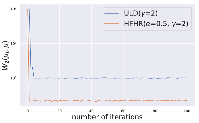
(a) 1D Gaussian

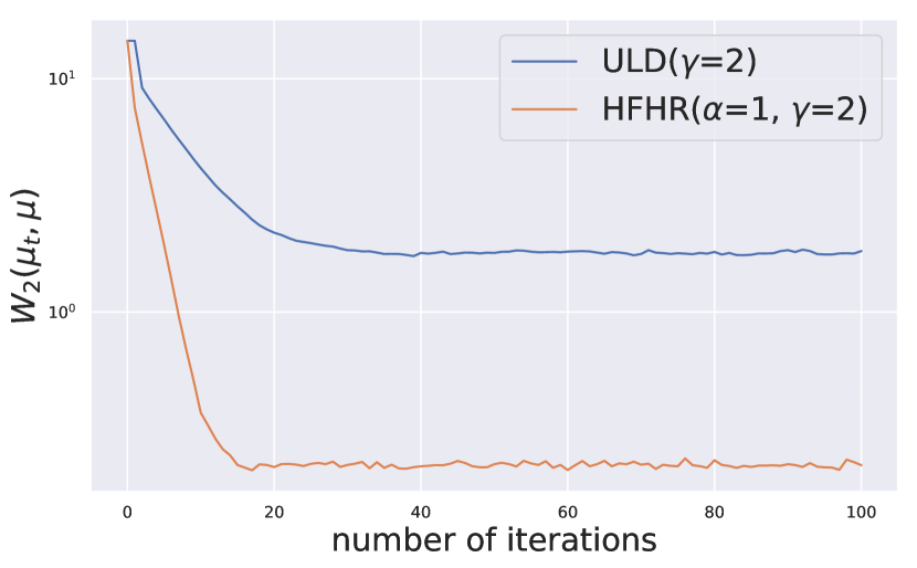
(b) 2D Gaussian($m=0.1$)

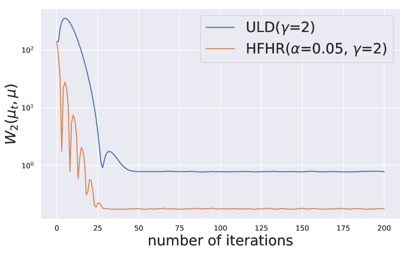
(c) 2D Gaussian($m=10$)

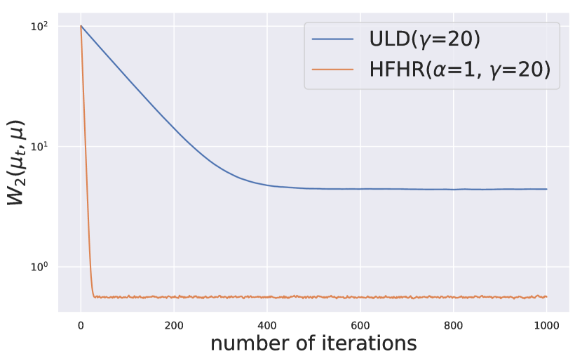
(d) 100D Gaussian

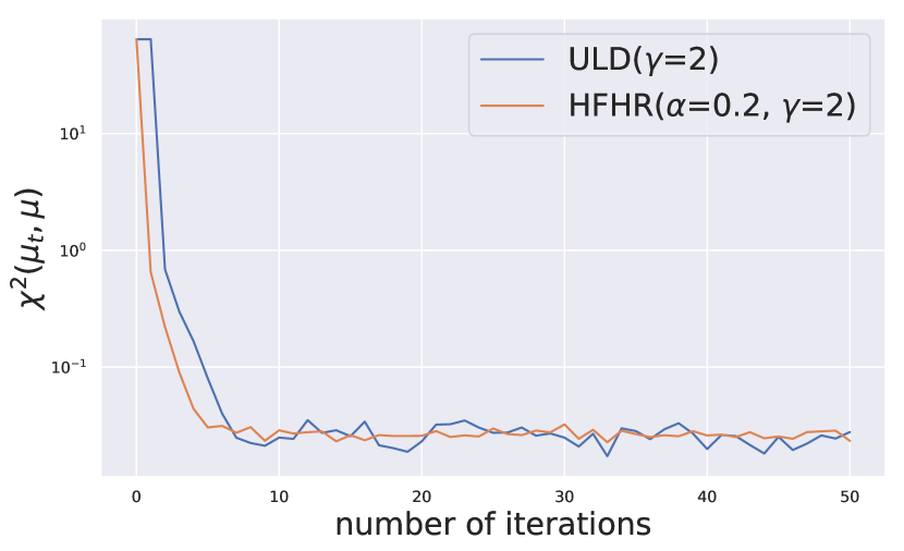
(e) Convex

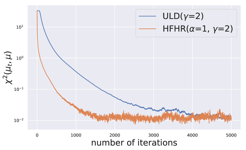
(f) Perturbed

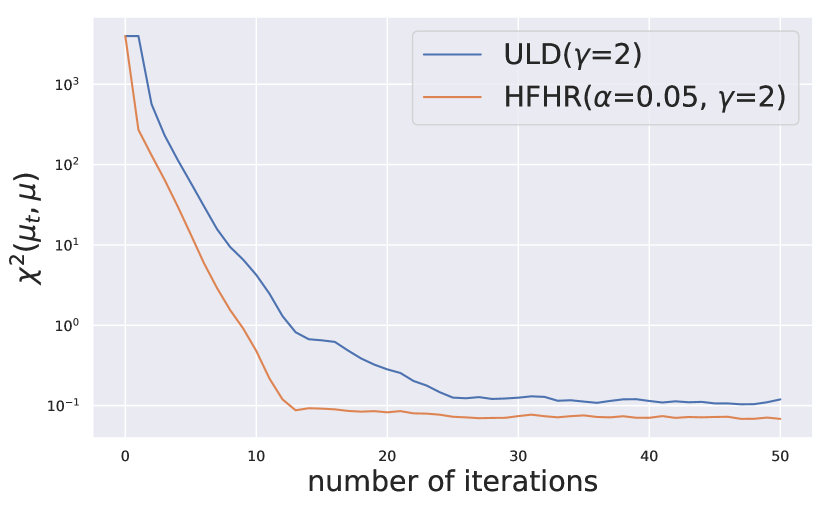
(g) Bi-modal

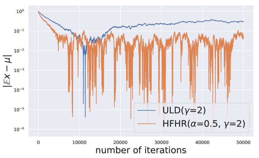
(h) 2D Rosenbrock

Figure 1: (a) $f_{1}\,(h=2)$. (b) $f_{2}\,(h=2)$. (c) $f_{3}\,(h=2.5)$. (d)$f_{4}\,(h=0.2)$. (e) $f_{5}\,(h=0.5)$. (f) $f_{6}\,(h=0.001)$. (g) $f_{7}\,(h=0.1)$. (h) $f_{8}\,(h=0.005)$. $y$-axes are in log scale.

We first test 8 target distributions with simple, yet representative potential functions, summarized in Table 1. For Gaussian targets, smoothness coefficient $L$ is available, hence we take $\gamma=2\sqrt{L}$ as suggested in Dalalyan & Riou-Durand (2020). To be consistent with Thm.5.2, closeness is measured in $W_{2}$ which has closed-form expression between Gaussians. For non-Gaussians, we empirically set $\gamma=2$ and measure sample quality by $\chi^{2}$ divergence with densities empiricially approximated by histograms. For the special case of $f_{8}(x,y)$, note approximating its density using a uniform-mesh-based histogram is either inaccurate or requiring the mesh to be very fine due to high nonconvexity, and we thus report the error in the $x$ component $|\mathbb{E}x-\mu|$ instead, where $\mu$ is the true mean of $x$-component. Each algorithm uses 10,000 independent realizations for empirical estimations.

Results are in Fig.1. The improvement by HFHR correction can be clearly seen, although note that we did not optimize over $\alpha,\gamma$ values but simply chose the same $\gamma$ across ULD and HFHR and an arbitrary $\alpha$ additionally for HFHR. Step size $h$ however is tuned so that it is near the stability limit of ULD algorithm, and then HFHR uses the same $h$. In the next section we’ll optimize over all possible parameters so that ULD at its best performance can be compared with.

6.2 A Nonlinear Case Study: Consistency with Theory

This section numerically verifies, more systematically, that $\alpha\neq 0$ (i.e. HFHR correction) accelerates the convergence, and optimal $\alpha$ exists (see Rmk.5.5), for which the acceleration is rather significant. In addition, how HFHR algorithm scales with the dimension is also of importance in a machine learning context, and thus the $\mathcal{O}(\sqrt{d})$ dependence given by Thm.5.2 (in $C$, which is also inherited by Cor.5.4 in the iteration complexity) will also be confirmed.

For the purpose of checking dimension dependence, we will not use Gaussian targets, because otherwise HFHR will decouple across different (orthogonal) dimensions, in which case an $\mathcal{O}(\sqrt{d})$ dependence is trivially true as a consequence of using $W_{2}$ for quantifying statistical accuracy. Instead, we consider the potential in Li et al. (2022b) which is not additive across dimensions, namely $f(\boldsymbol{x})=\log\left(e^{x_{1}}+\cdots+e^{x_{d}}\right)+\frac{1}{2}\mathinner{\!\left\lVert\boldsymbol{x}\right\rVert}^{2}.$ This is still a strongly convex function satisfying the assumption in Thm.5.2. The corresponding target is not Gaussian, we no longer have a closed form expression for $W_{2}$ distance, and it is computationally expensive to approximate this distance by samples. Therefore, we follow Li et al. (2022b) and use the error of mean instead as a surrogate because $\displaystyle\mathinner{\!\left\lVert\mathbb{E}_{\mu_{k}}\boldsymbol{q}-\mathbb{E}_{\mu}\boldsymbol{q}\right\rVert}\leq W_{2}(\mu_{k},\mu)$ and hence the bound in Eq.(8) also applies to the error in mean, and so does the iteration complexity bound in Eq.(10).

Fig.2 compares HFHR (Alg.1) with ULD (KLMC) in terms of iteration complexity. To show that the acceleration of HFHR is not an artifact of time rescaling (which would disappear after discretization as the stability limit changes accordingly), we optimize over $h$ (by pushing both ULD and HFHR to their respective largest $h$ values that still allow monotonic convergence at a large scale), as well as $\gamma$ values, and compare the resulting best mixing times.

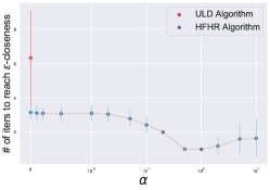
Figure 2: Improvement of Algorithm 1 over ULD algorithm in iteration complexity. (vertical bar = 1 standard deviation)

More specifically, we choose the initial measure to be Dirac at $(100\times\boldsymbol{1}_{d},\boldsymbol{0}_{d})$, where $\boldsymbol{1}_{d},\boldsymbol{0}_{d}$ are $d$-dim. vectors filled with $1$ and $0$ respectively. $d=10$. We pick threshold $\epsilon=0.1$, and for each $\alpha\in\{$0, 0.001, 0.002, 0.005, 0.01, 0.02, 0.05, 0.1, 0.2, 0.5, 1, 2, 5, 10, 20, 50, 100$\}$, we try all combinations of $(\gamma,h)\in\{$0.1, 0.2, 0.5, 1, 2, 5, 10, 20, 50, 100$\}\times\left\{0.1\times[50]\right\}$ for Algorithm 1 (we also run ULD algorithm when $\alpha=0$), and empirically find the best combination that requires the fewest iterations to meet $\mathinner{\!\left\lVert\mathbb{E}_{\mu_{k}}\boldsymbol{q}-\mathbb{E}_{\mu}\boldsymbol{q}\right\rVert}\leq\epsilon$. We find that $h=5$ already surpasses the stability limit of ULD algorithm, hence the range of step size covers the largest step size that are practically usable for ULD algorithm. 100,000 independent realizations are used (evenly spread to 100 different randomization seeds).

When $\alpha>0$, HFHR algorithm consistently outperforms ULD algorithm under optimized parameters (note it also does so when $\alpha=0$ because Alg.1 uses a efficiency-wise comparable but more accurate discretization than ULD algorithm). In particular, when $\alpha=0.5$ and $1$, which are empirically best values found for this experiment, HFHR achieves the specified $\epsilon$-closeness nearly 6$\times$ times faster than ULD, and its decreased mixing time (compared to $\alpha=0$ for the same algorithm) is consistent with the $\approx 0.46$ factor in Rmk.5.5). These corroborate that the $\alpha\neq 0$ HFHR correction effect is genuine, and the resulting acceleration can be significant.

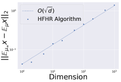
Figure 3: $\sqrt{d}$ dependence of sampling error of Alg.1

Regarding dimension dependence, Thm.5.2 states the HFHR sampling error is upper bounded by its discretization error, which is linear in $\sqrt{d}$. This is consistent with empirical observation in Fig.3, where we experiment with $d\in\left\{1,2,5,10,20,50,100,200,500,1000\right\}$. For each $d$, we fix $\gamma=2,\alpha=1,h=0.1$, choose a large enough $T=10$, run 1,000 independent realizations of HFHR algorithm, and estimate the sampling error using the surrogate.

6.3 Bayesian Neural Network

To test the efficacy of HFHR on practical non-convex problems, we consider Bayesian neural network (BNN) which is a compelling learning model (Wilson, 2020); however, the focus won’t be on its learning capability, and instead we just consider its training, which amounts to a real-life, high-dimensional, multi-modal example of sampling tasks. It no longer satisfies the conditions of our analysis, and our goal is to show HFHR still accelerates. We use fully-connected network with [22, 10, 2] neurons, ReLU, standard Gaussian prior for all parameters, and compare ULD and HFHR on UCI data set Parkinson (Dua & Graff, 2017).

Choices of hyper-parameter for Algorithm 1 and ULD algorithm are systematically investigated. For each pair $(\gamma,\alpha)\in\{0.1,0.5,1,5,10,50,100\}^{2}$, we empirically tune the step size to the stability limit of ULD algorithm, simulate 1,000 independent realizations, and use the ensemble to conduct Bayesian posterior prediction. HFHR will then use the same step size. For each $\gamma$, we plot the negative log likelihood of HFHR algorithm (with different $\alpha$ choices) and ULD algorithm on training and test data in Figure 4.

Fig.4 indicates that HFHR converges significantly faster than ULD in a wide range of setups. Obviously, the log-strongly-concave assumption required in Thm.5.2 does not hold for multimodal target distributions. However, this numerical result shows that HFHR still accelerates ULD for highly complex models such as BNN, even when there is no obvious theoretical guarantee. It showcases the applicability and effectiveness of HFHR as a general sampling algorithm.

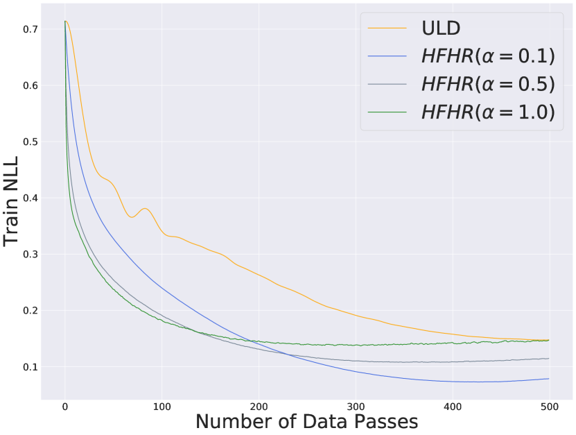
(a) $\gamma=0.1\,(h=0.005)$

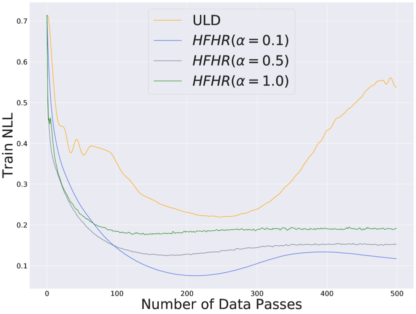
(b) $\gamma=0.1\,(h=0.01)$

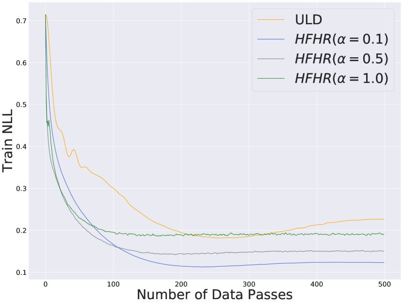
(c) $\gamma=1\,(h=0.01)$

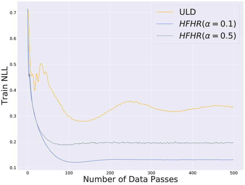
(d) $\gamma=1\,(h=0.02)$

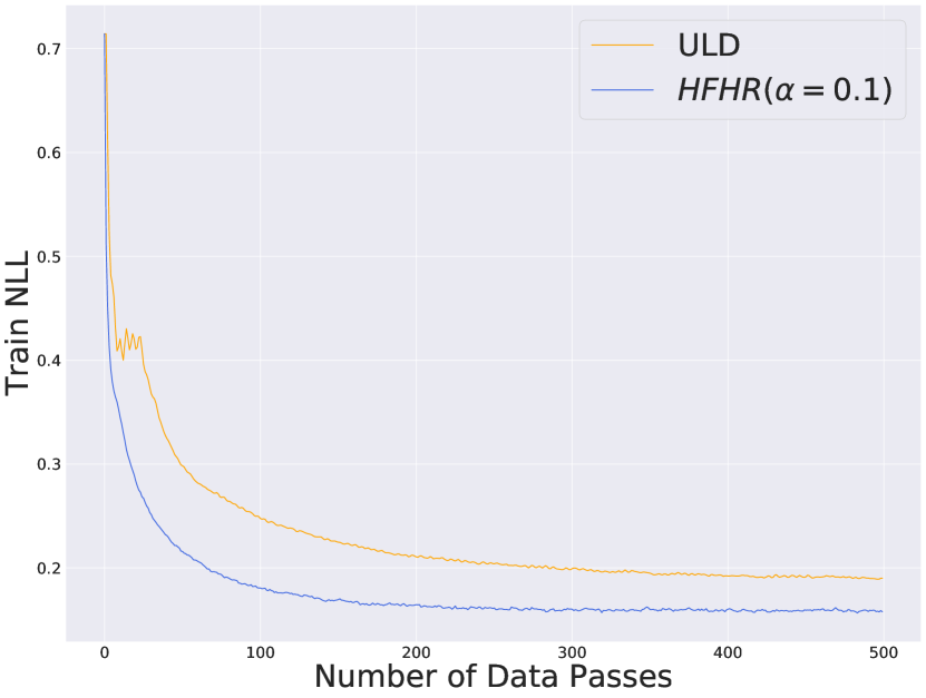
(e) $\gamma=10\,(h=0.05)$

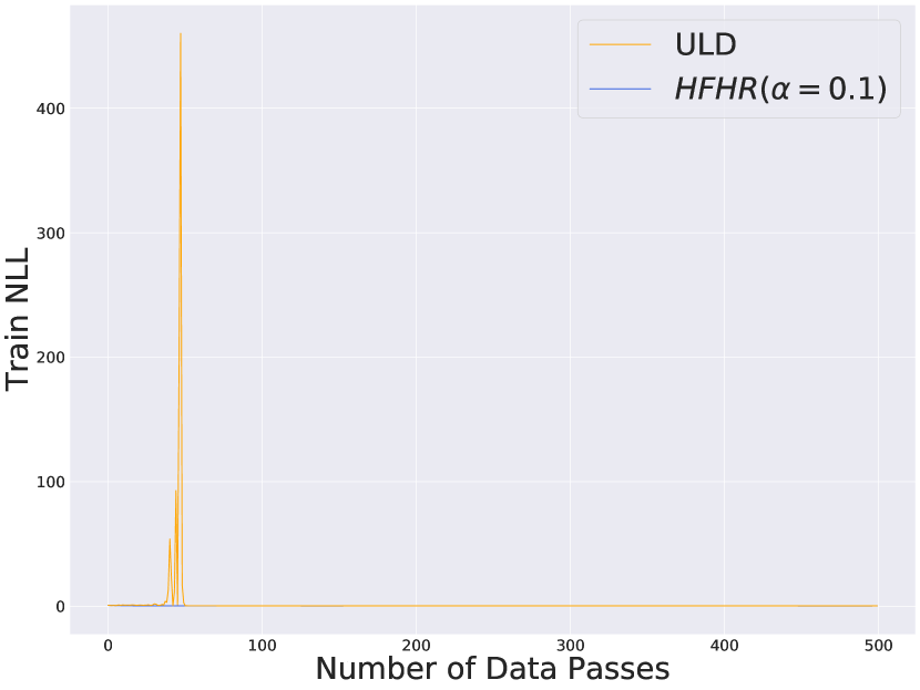
(f) $\gamma=10\,(h=0.1)$

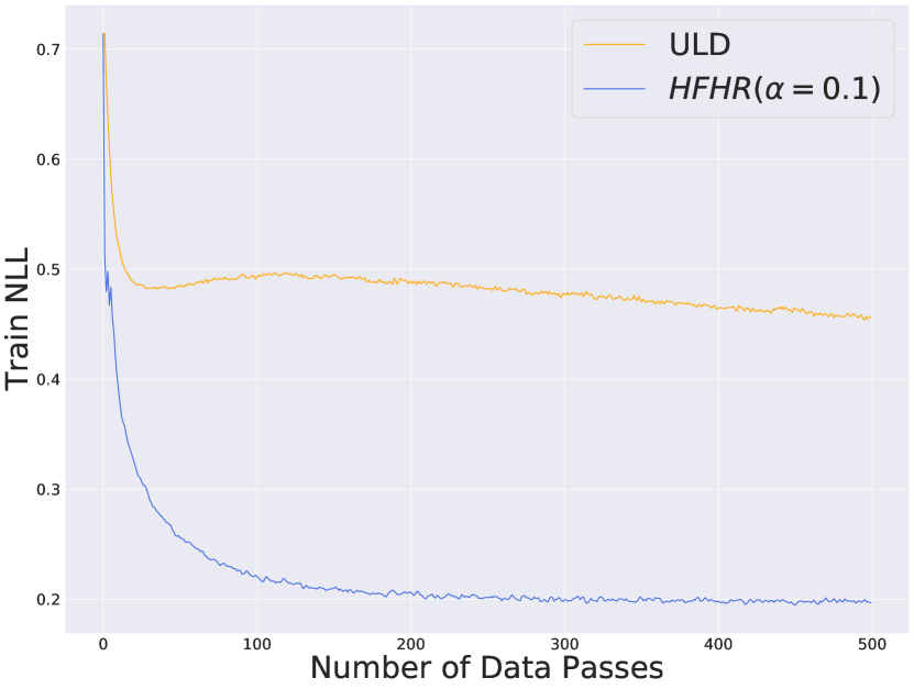
(g) $\gamma=100\,(h=0.1)$

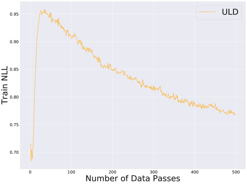
(h) $\gamma=100\,(h=0.2)$

Figure 4: Training Negative Log-Likelihood (NLL) for various $\gamma$. Left column uses step sizes that are close to the stability limit of ULD algorithm, as further increased step size in right column no longer gives stability/monotonicity. Unstable cases where $\alpha$ is too large are not drawn (recall $\alpha,\gamma,h$ constrain each other; see e.g., Rmk.5.5 for intuitions in convex setups).

7 Conclusion and Discussion

This paper proposes HFHR dynamics, a NAG-optimizer-based diffusion process. Its discretizations give a family of accelerated sampling algorithms. To demonstrate the acceleration enabled by HFHR, the geometric ergodicity of HFHR (both the continuous and discretized versions) is quantified, and its convergence is provably faster than Underdamped Langevin Dynamics, which by itself is often already considered as an accelerated version of Overdamped Langevin Dynamics. Since HFHR adopts a new perspective, which is to turn the finite learning rate advantage of NAG-SC optimizer into a sampling counterpart, there are a number of directions in which this work can be extended: (i) HFHR dynamics can be discretized in different ways resulting in different algorithms. Two popular discretizations are considered here and one theoretically analyzed, but other discretizations could also be used and possibly lead to favorable performances. (ii) To scale HFHR up to large data sets, full gradient may be replaced by stochastic gradient (SG) — how to quantify, and hence optimize the performance of SG-HFHR? (iii) Can the generalization ability of HFHR-trained learning models (e.g., BNN) be quantified, and how does it compare with that by LMC, KLMC, or other dynamics-based samplers? These will be future work.

Appendix A Additional Notations

We introduce a few notations that are used in the main text as well as some proof. When $\nabla f$ is $L$-Lipschitz, the drift term $\begin{bmatrix}\boldsymbol{p}-\alpha\nabla f(\boldsymbol{q})\\ -\gamma\boldsymbol{p}-\nabla f(\boldsymbol{q})\end{bmatrix}$ in HFHR dynamics is also $L^{\prime}$-Lipschitz, as proved in Lemma D.3, where

$$L^{\prime}=\sqrt{2}\max\left\{\sqrt{1+\alpha^{2}}\max\left\{\frac{1}{\sqrt{2}},L\right\},\sqrt{1+\gamma^{2}}\right\}.$$

We show in Lemma D.5 that a linear-transformed HFHR dynamics satisfies the nice contraction property, the linear transformation $P$ we use is defined as

$$P=\begin{bmatrix}\gamma I&I\\ 0&\sqrt{1+\alpha\gamma}I\end{bmatrix}\in\mathbb{R}^{2d\times 2d}.$$

Denote the largest and the smallest singular value of $P$ by

$$\sigma_{\text{max}}= \sqrt{\frac{\alpha\gamma}{2}+\frac{\gamma^{2}}{2}+\frac{\sqrt{\alpha^{2}\gamma^{2}-2\alpha\gamma^{3}+4\alpha\gamma+\gamma^{4}+4}}{2}+1},$$

$$\sigma_{\text{min}}= s\sqrt{\frac{\alpha\gamma}{2}+\frac{\gamma^{2}}{2}-\frac{\sqrt{\alpha^{2}\gamma^{2}-2\alpha\gamma^{3}+4\alpha\gamma+\gamma^{4}+4}}{2}+1}$$

and its condition number by

$$\kappa^{\prime}=\frac{\sigma_{\text{max}}}{\sigma_{\text{min}}}=\sqrt{\frac{\frac{\alpha\gamma}{2}+\frac{\gamma^{2}}{2}+\frac{\sqrt{\alpha^{2}\gamma^{2}-2\alpha\gamma^{3}+4\alpha\gamma+\gamma^{4}+4}}{2}+1}{\frac{\alpha\gamma}{2}+\frac{\gamma^{2}}{2}-\frac{\sqrt{\alpha^{2}\gamma^{2}-2\alpha\gamma^{3}+4\alpha\gamma+\gamma^{4}+4}}{2}+1}}.$$

The rate $\lambda^{\prime}$ of exponential convergence of transformed HFHR dynamics is characterized in Lemma D.5 and is defined as

$$\lambda^{\prime}=\min\left\{\frac{m}{\gamma}+\alpha m,\frac{\gamma^{2}-L}{\gamma}\right\}$$

given that $\gamma^{2}>L$.

Appendix B Proofs for the Continuous Dynamics

Notations and definitions can be found in Sec.3.

B.1 Proof of Theorem 4.1

Proof.

The Fokker-Plank equation of HFHR is given by

$$\partial_{t}\rho_{t}=-\nabla_{\boldsymbol{x}}\cdot\left(\begin{bmatrix}\boldsymbol{p}\\ -\nabla f(\boldsymbol{q})\end{bmatrix}\rho_{t}\right)+\alpha\left(\nabla_{\boldsymbol{q}}\cdot(\nabla f(\boldsymbol{q})\rho_{t})+\Delta_{\boldsymbol{q}}\rho_{t}\right)+\gamma\left(\nabla_{\boldsymbol{p}}\cdot(\boldsymbol{p}\rho_{t})+\Delta_{\boldsymbol{p}}\rho_{t}\right)$$

where $\nabla_{\boldsymbol{x}}=(\nabla_{\boldsymbol{q}},\nabla_{\boldsymbol{p}})$. For $\pi\propto e^{-f(\boldsymbol{q})-\frac{1}{2}\|\boldsymbol{p}\|^{2}}$, we have

$$\nabla_{\boldsymbol{x}}\cdot\left(\begin{bmatrix}\boldsymbol{p}\\ -\nabla f(\boldsymbol{q})\end{bmatrix}\pi\right)=\langle\begin{bmatrix}\boldsymbol{p}\\ -\nabla f(\boldsymbol{q})\end{bmatrix},\nabla_{\boldsymbol{x}}\pi\rangle=0,$$

$$\Delta_{\boldsymbol{q}}\pi=-\nabla_{\boldsymbol{q}}\cdot(\pi\nabla f(\boldsymbol{q}))$$

$$\Delta_{\boldsymbol{p}}\pi=-\nabla_{\boldsymbol{p}}\cdot(\pi\boldsymbol{p})$$

Therefore $\partial_{t}\pi=0$ and hence $\pi$ is the invariant distribution of HFHR. ∎

B.2 Proof of Theorem 5.1

Proof.

Consider two copies of HFHR that are driven by the same Brownian motion

$$\begin{cases}d\boldsymbol{q}_{t}=(\boldsymbol{p}_{t}-\alpha\nabla f(\boldsymbol{q}_{t}))dt+\sqrt{2\alpha}d\boldsymbol{B}^{1}_{t}\\ d\boldsymbol{p}_{t}=(-\gamma\boldsymbol{p}_{t}-\nabla f(\boldsymbol{q}_{t}))dt+\sqrt{2\gamma}d\boldsymbol{B}^{2}_{t}\end{cases},\quad\begin{cases}d\tilde{\boldsymbol{q}}_{t}=(\tilde{\boldsymbol{p}}_{t}-\alpha\nabla f(\tilde{\boldsymbol{q}}_{t}))dt+\sqrt{2\alpha}d\boldsymbol{B}^{1}_{t}\\ d\tilde{\boldsymbol{p}_{t}}=(-\gamma\tilde{\boldsymbol{p}}_{t}-\nabla f(\tilde{\boldsymbol{q}}_{t}))dt+\sqrt{2\gamma}d\boldsymbol{B}^{2}_{t}\end{cases},$$

where we set $(\tilde{\boldsymbol{q}}_{0},\tilde{\boldsymbol{p}}_{0})\sim\pi$, $\boldsymbol{p}_{0}=\tilde{\boldsymbol{p}}_{0}$ and $\boldsymbol{q}_{0}$ such that

$$W_{2}^{2}(\mu_{0},\mu)=\mathbb{E}\left[\|\boldsymbol{q}_{0}-\tilde{\boldsymbol{q}}_{0}\|^{2}_{2}\right],\quad\boldsymbol{q}_{0}\sim\mu_{0}$$

Denote $\begin{bmatrix}\boldsymbol{\phi}_{t}\\ \boldsymbol{\psi}_{t}\end{bmatrix}=P\begin{bmatrix}\boldsymbol{q}_{t}-\tilde{\boldsymbol{q}}_{t}\\ \boldsymbol{p}_{t}-\tilde{\boldsymbol{p}}_{t}\end{bmatrix}$ where $P$ is defined in Appendix A. By Lemma D.5 and the assumption on $\alpha,\gamma$, we have

$$\mathinner{\!\left\lVert\begin{bmatrix}\boldsymbol{\phi}_{t}\\ \boldsymbol{\psi}_{t}\end{bmatrix}\right\rVert}^{2}\leq e^{-2(\frac{m}{\gamma}+m\alpha)t}\mathinner{\!\left\lVert\begin{bmatrix}\boldsymbol{\phi}_{0}\\ \boldsymbol{\psi}_{0}\end{bmatrix}\right\rVert}^{2}.$$

Therefore we obtain

$$W_{2}^{2}(\mu_{t},\mu)= \inf_{(\boldsymbol{q}_{t},\tilde{\boldsymbol{q}}_{t})\sim\Pi(\mu_{t},\mu)}\mathbb{E}\mathinner{\!\left\lVert\boldsymbol{q}_{t}-\tilde{\boldsymbol{q}}_{t}\right\rVert}^{2}$$

$$\leq \inf_{(\boldsymbol{q}_{t},\tilde{\boldsymbol{q}}_{t})\sim\Pi(\mu_{t},\mu),(\boldsymbol{p}_{t},\tilde{\boldsymbol{p}}_{t})\sim\Pi(\nu_{t},\nu)}\mathbb{E}\mathinner{\!\left\lVert\begin{bmatrix}\boldsymbol{q}_{t}-\tilde{\boldsymbol{q}}_{t}\\ \boldsymbol{p}_{t}-\tilde{\boldsymbol{p}}_{t}\end{bmatrix}\right\rVert}^{2}$$

$$\leq \mathbb{E}\|P^{-1}\|_{2}^{2}\mathinner{\!\left\lVert\begin{bmatrix}\boldsymbol{\phi}_{t}\\ \boldsymbol{\psi}_{t}\end{bmatrix}\right\rVert}^{2}$$

$$\leq \mathbb{E}\|P^{-1}\|_{2}^{2}e^{-2(\frac{m}{\gamma}+m\alpha)t}\mathinner{\!\left\lVert\begin{bmatrix}\boldsymbol{\phi}_{0}\\ \boldsymbol{\psi}_{0}\end{bmatrix}\right\rVert}^{2}$$

$$\leq (\kappa^{\prime})^{2}e^{-2(\frac{m}{\gamma}+m\alpha)t}\mathinner{\!\left\lVert\begin{bmatrix}\boldsymbol{q}_{0}-\tilde{\boldsymbol{q}}_{0}\\ \boldsymbol{p}_{0}-\tilde{\boldsymbol{p}}_{0}\end{bmatrix}\right\rVert}^{2}$$

$$= (\kappa^{\prime})^{2}e^{-2(\frac{m}{\gamma}+m\alpha)t}W_{2}^{2}(\mu_{0},\mu)$$

Taking square root yields the desired result.

∎

Appendix C Arbitrary Long Time Discretization Error of Algorithm 1

Theorem C.1.

Under Conditions A3.1 and further assume the function $\nabla\Delta f$ grows at most linearly, i.e., $\mathinner{\!\left\lVert\nabla\Delta f(\boldsymbol{q})\right\rVert}\leq G\sqrt{1+\mathinner{\!\left\lVert\boldsymbol{q}\right\rVert}^{2}},\forall\boldsymbol{q}\in\mathbb{R}^{d}$. Also suppose $\gamma$ in HFHR dynamics satisfy $\gamma^{2}>L$. Then there exist $C,h_{0}>0$, such that for $0<h\leq h_{0}$, we have

$$\left(\mathbb{E}\mathinner{\!\left\lVert\boldsymbol{x}_{k}-\bar{\boldsymbol{x}}_{k}\right\rVert}^{2}\right)^{\frac{1}{2}}\leq Ch$$

where $\bar{\boldsymbol{x}}_{k}$ is the $k$-th iterate of Algorithm 1 with step size $h$ starting from $\boldsymbol{x}_{0}$, $\boldsymbol{x}_{k}$ is the solution of HFHR dynamics at time $kh$, starting from $\boldsymbol{x}_{0}$. This result holds uniformly for all $k\geq 0$ and $k$ can go to $\infty$. In particular, $C=\mathcal{O}(\sqrt{d})$ and if $\gamma-\frac{L+m}{\gamma}\geq m\alpha$, then there exists $b>0$, independent of $\alpha$ and is of order $\mathcal{O}(\sqrt{d})$, such that

$$C\leq\frac{b}{m}(\alpha^{2}-\frac{\alpha}{\gamma}+\frac{1}{\gamma^{2}}).$$ (11)

Proof.

Denote $t_{k}=kh$, the solution of the HFHR dynamics at time $t$ by $\boldsymbol{x}_{0,\boldsymbol{x}_{0}}(t)$, the $k$-th iterates of the Strang’s splitting method of HFHR dynamics by $\bar{\boldsymbol{x}}_{0,\boldsymbol{x}_{0}}(kh)$. Both $\boldsymbol{x}_{0,\boldsymbol{x}_{0}}(t)$ and $\bar{\boldsymbol{x}}_{0,\boldsymbol{x}_{0}}(kh)$ start from the same initial value $\boldsymbol{x}_{0}$. The linear transformation $P$ defined in Appendix A, transforms the solution of HFHR dynamics into $\boldsymbol{y}_{0,P\boldsymbol{x}_{0}}(t)=P\boldsymbol{x}_{0,\boldsymbol{x}_{0}}(t)$ and the Strang’s splitting discretization of HFHR into $\bar{\boldsymbol{y}}_{0,P\boldsymbol{x}_{0}}(t)=P\bar{\boldsymbol{x}}_{0,\boldsymbol{x}_{0}}(t)$.

For the ease of notation, we write $\boldsymbol{y}_{0,\boldsymbol{y}_{0}}(t_{k})$ as $\boldsymbol{y}_{k}$ and $\bar{\boldsymbol{y}}_{0,\boldsymbol{y}_{0}}(t_{k})$ as $\bar{\boldsymbol{y}}_{k}$. We have the following identity

$$\mathbb{E}\mathinner{\!\left\lVert\boldsymbol{y}_{k+1}-\bar{\boldsymbol{y}}_{k+1}\right\rVert}^{2}= \mathbb{E}\mathinner{\!\left\lVert\boldsymbol{y}_{t_{k},\boldsymbol{y}_{k}}(h)-\bar{\boldsymbol{y}}_{t_{k},\bar{\boldsymbol{y}}_{k}}(h)\right\rVert}^{2}$$

$$= \mathbb{E}\mathinner{\!\left\lVert\boldsymbol{y}_{t_{k},\boldsymbol{y}_{k}}(h)-\boldsymbol{y}_{t_{k},\bar{\boldsymbol{y}}_{k}}(h)+\boldsymbol{y}_{t_{k},\bar{\boldsymbol{y}}_{k}}(h)-\bar{\boldsymbol{y}}_{t_{k},\bar{\boldsymbol{y}}_{k}}(h)\right\rVert}^{2}$$

$$= \underbrace{\mathbb{E}\mathinner{\!\left\lVert\boldsymbol{y}_{t_{k},\boldsymbol{y}_{k}}(h)-\boldsymbol{y}_{t_{k},\bar{\boldsymbol{y}}_{k}}(h)\right\rVert}^{2}}_{\leavevmode\hbox to11.75pt{\vbox to11.75pt{\text{[drawing]}}}}+\underbrace{\mathbb{E}\mathinner{\!\left\lVert\boldsymbol{y}_{t_{k},\bar{\boldsymbol{y}}_{k}}(h)-\bar{\boldsymbol{y}}_{t_{k},\bar{\boldsymbol{y}}_{k}}(h)\right\rVert}^{2}}_{\leavevmode\hbox to11.75pt{\vbox to11.75pt{\text{[drawing]}}}}$$

$$+ 2\underbrace{\mathbb{E}\left\langle\boldsymbol{y}_{t_{k},\boldsymbol{y}_{k}}(h)-\boldsymbol{y}_{t_{k},\bar{\boldsymbol{y}}_{k}}(h),\boldsymbol{y}_{t_{k},\bar{\boldsymbol{y}}_{k}}(h)-\bar{\boldsymbol{y}}_{t_{k},\bar{\boldsymbol{y}}_{k}}(h)\right\rangle}_{\leavevmode\hbox to11.75pt{\vbox to11.75pt{\text{[drawing]}}}}$$

By Lemma D.5, when $0<h<\frac{1}{2\lambda^{\prime}}$, term can be upper bounded as

$$\mathbb{E}\mathinner{\!\left\lVert\boldsymbol{y}_{t_{k},\boldsymbol{y}_{k}}(h)-\boldsymbol{y}_{t_{k},\bar{\boldsymbol{y}}_{k}}(h)\right\rVert}^{2}\leq e^{-2\lambda^{\prime}h}\mathbb{E}\mathinner{\!\left\lVert\boldsymbol{y}_{k}-\bar{\boldsymbol{y}}_{k}\right\rVert}^{2}$$

$$\leq \left(1-2\lambda^{\prime}h+2(\lambda^{\prime})^{2}h^{2}\right)\mathbb{E}\mathinner{\!\left\lVert\boldsymbol{y}_{k}-\bar{\boldsymbol{y}}_{k}\right\rVert}^{2}$$

$$\leq \left(1-\lambda^{\prime}h\right)\mathbb{E}\mathinner{\!\left\lVert\boldsymbol{y}_{k}-\bar{\boldsymbol{y}}_{k}\right\rVert}^{2}$$

where the second inequality is due to $e^{-x}\leq 1-x+\frac{x^{2}}{2},\forall x>0$.

For term , we have by Lemma D.8 that

$$\mathbb{E}\mathinner{\!\left\lVert\boldsymbol{y}_{t_{k},\bar{\boldsymbol{y}}_{k}}(h)-\bar{\boldsymbol{y}}_{t_{k},\bar{\boldsymbol{y}}_{k}}(h)\right\rVert}^{2}\leq\sigma_{\text{max}}^{2}\,\mathbb{E}\mathinner{\!\left\lVert\boldsymbol{x}_{t_{k},\bar{\boldsymbol{x}}_{k}}(h)-\bar{\boldsymbol{x}}_{t_{k},\bar{\boldsymbol{x}}_{k}}(h)\right\rVert}^{2}\leq\sigma_{\text{max}}^{2}\,C_{2}^{2}h^{3}$$

where $\sigma_{\text{max}}$ is the largest singular value of matrix $P$.

For term , we have by Lemma D.1 that

$$2\mathbb{E}\left\langle\boldsymbol{y}_{t_{k},\boldsymbol{y}_{k}}(h)-\boldsymbol{y}_{t_{k},\bar{\boldsymbol{y}}_{k}}(h),\boldsymbol{y}_{t_{k},\bar{\boldsymbol{y}}_{k}}(h)-\bar{\boldsymbol{y}}_{t_{k},\bar{\boldsymbol{y}}_{k}}(h)\right\rangle$$

$$= 2\mathbb{E}\left\langle\boldsymbol{y}_{k}-\bar{\boldsymbol{y}}_{k}+\boldsymbol{z},\boldsymbol{y}_{t_{k},\bar{\boldsymbol{y}}_{k}}(h)-\bar{\boldsymbol{y}}_{t_{k},\bar{\boldsymbol{y}}_{k}}(h)\right\rangle$$

$$= \underbrace{2\mathbb{E}\left\langle\boldsymbol{y}_{k}-\bar{\boldsymbol{y}}_{k},\boldsymbol{y}_{t_{k},\bar{\boldsymbol{y}}_{k}}(h)-\bar{\boldsymbol{y}}_{t_{k},\bar{\boldsymbol{y}}_{k}}(h)\right\rangle}_{\leavevmode\hbox to14.27pt{\vbox to14.27pt{\text{[drawing]}}}}+\underbrace{2\mathbb{E}\left\langle\boldsymbol{z},\boldsymbol{y}_{t_{k},\bar{\boldsymbol{y}}_{k}}(h)-\bar{\boldsymbol{y}}_{t_{k},\bar{\boldsymbol{y}}_{k}}(h)\right\rangle}_{\leavevmode\hbox to14.83pt{\vbox to14.83pt{\text{[drawing]}}}}$$

For term , by the tower property of conditional expectation, we have

$$2\mathbb{E}\left\langle\boldsymbol{y}_{k}-\bar{\boldsymbol{y}}_{k},\boldsymbol{y}_{t_{k},\bar{\boldsymbol{y}}_{k}}(h)-\bar{\boldsymbol{y}}_{t_{k},\bar{\boldsymbol{y}}_{k}}(h)\right\rangle= 2\mathbb{E}\left[\mathbb{E}\left[\left\langle\boldsymbol{y}_{k}-\bar{\boldsymbol{y}}_{k},\boldsymbol{y}_{t_{k},\bar{\boldsymbol{y}}_{k}}(h)-\bar{\boldsymbol{y}}_{t_{k},\bar{\boldsymbol{y}}_{k}}(h)\right\rangle\bigg{|}\mathcal{F}_{k}\right]\right]$$

$$= 2\mathbb{E}\left\langle\boldsymbol{y}_{k}-\bar{\boldsymbol{y}}_{k},\mathbb{E}\left[\boldsymbol{y}_{t_{k},\bar{\boldsymbol{y}}_{k}}(h)-\bar{\boldsymbol{y}}_{t_{k},\bar{\boldsymbol{y}}_{k}}(h)\bigg{|}\mathcal{F}_{k}\right]\right\rangle$$

$$\leq 2\sqrt{\mathbb{E}\mathinner{\!\left\lVert\boldsymbol{y}_{k}-\bar{\boldsymbol{y}}_{k}\right\rVert}^{2}}\sqrt{\mathbb{E}\mathinner{\!\left\lVert\mathbb{E}\left[\boldsymbol{y}_{t_{k},\bar{\boldsymbol{y}}_{k}}(h)-\bar{\boldsymbol{y}}_{t_{k},\bar{\boldsymbol{y}}_{k}}(h)\bigg{|}\mathcal{F}_{k}\right]\right\rVert}^{2}}$$

$$\leq 2\sqrt{\mathbb{E}\mathinner{\!\left\lVert\boldsymbol{y}_{k}-\bar{\boldsymbol{y}}_{k}\right\rVert}^{2}}\sqrt{\sigma_{\text{max}}^{2}\mathbb{E}\mathinner{\!\left\lVert\mathbb{E}\left[\boldsymbol{x}_{t_{k},\bar{\boldsymbol{x}}_{k}}(h)-\bar{\boldsymbol{x}}_{t_{k},\bar{\boldsymbol{x}}_{k}}(h)\bigg{|}\mathcal{F}_{k}\right]\right\rVert}^{2}}$$

$$\leq 2\sqrt{\mathbb{E}\mathinner{\!\left\lVert\boldsymbol{y}_{k}-\bar{\boldsymbol{y}}_{k}\right\rVert}^{2}}\sqrt{\sigma_{\text{max}}^{2}C_{1}^{2}h^{4}}$$

$$\leq 2\sigma_{\text{max}}C_{1}\sqrt{\mathbb{E}\mathinner{\!\left\lVert\boldsymbol{y}_{k}-\bar{\boldsymbol{y}}_{k}\right\rVert}^{2}}h^{2}.$$

For term , when $0<h<\frac{1}{4L^{\prime\prime}}$we have by Lemma D.1 and Lemma D.8

$$2\mathbb{E}\left\langle\boldsymbol{z},\boldsymbol{y}_{t_{k},\bar{\boldsymbol{y}}_{k}}(h)-\bar{\boldsymbol{y}}_{t_{k},\bar{\boldsymbol{y}}_{k}}(h)\right\rangle\leq 2\sqrt{\mathbb{E}\mathinner{\!\left\lVert\boldsymbol{z}\right\rVert}^{2}}\sqrt{\mathbb{E}\mathinner{\!\left\lVert\boldsymbol{y}_{t_{k},\bar{\boldsymbol{y}}_{k}}(h)-\bar{\boldsymbol{y}}_{t_{k},\bar{\boldsymbol{y}}_{k}}(h)\right\rVert}^{2}}$$

$$= 2\sqrt{\mathbb{E}\mathinner{\!\left\lVert\boldsymbol{z}\right\rVert}^{2}}\sqrt{\mathbb{E}\left[\mathbb{E}\left[\mathinner{\!\left\lVert\boldsymbol{y}_{t_{k},\bar{\boldsymbol{y}}_{k}}(h)-\bar{\boldsymbol{y}}_{t_{k},\bar{\boldsymbol{y}}_{k}}(h)\right\rVert}^{2}\bigg{|}\mathcal{F}_{k}\right]\right]}$$

$$= 2\sqrt{\mathbb{E}\mathinner{\!\left\lVert\boldsymbol{z}\right\rVert}^{2}}\sqrt{\sigma_{\text{max}}^{2}\mathbb{E}\left[\mathbb{E}\left[\mathinner{\!\left\lVert\boldsymbol{x}_{t_{k},\bar{\boldsymbol{x}}_{k}}(h)-\bar{\boldsymbol{x}}_{t_{k},\bar{\boldsymbol{x}}_{k}}(h)\right\rVert}^{2}\bigg{|}\mathcal{F}_{k}\right]\right]}$$

$$\leq 2\sigma_{\text{max}}\sqrt{\tilde{C}\mathbb{E}\mathinner{\!\left\lVert\boldsymbol{y}_{k}-\bar{\boldsymbol{y}}_{k}\right\rVert}^{2}h^{2}}\sqrt{C_{2}^{2}h^{3}}$$

$$\leq 2\sigma_{\text{max}}C_{2}\sqrt{\tilde{C}}\sqrt{\mathbb{E}\mathinner{\!\left\lVert\boldsymbol{y}_{k}-\bar{\boldsymbol{y}}_{k}\right\rVert}^{2}}h^{\frac{5}{2}}$$

where $\tilde{C}=2\left(L^{\prime\prime}\right)^{2}=2(\kappa^{\prime})^{2}\left(L^{\prime}\right)^{2}$ is from Lemma D.1 and Lemma D.3.

Recall both $C_{1}$ and $C_{2}$ depend on $\mathinner{\!\left\lVert\boldsymbol{x}_{k}\right\rVert}$ and we would like to upper bound this term. To this end, consider $\tilde{\boldsymbol{x}}(t)$, a solution of HFHR dynamics with initial value $\tilde{\boldsymbol{x}}_{0}$ that follows the invariant distribution $\tilde{\boldsymbol{x}}_{0}\sim\pi$ and realizes $W_{2}(\pi_{0},\pi)$, i.e., $\mathbb{E}\mathinner{\!\left\lVert\tilde{\boldsymbol{x}}_{0}-\boldsymbol{x}_{0}\right\rVert}^{2}=W_{2}^{2}(\pi_{0},\pi)$.

Denote $\tilde{\boldsymbol{x}}_{k}=\tilde{\boldsymbol{x}}(kh)$ and $e_{k}=\left(\mathbb{E}\mathinner{\!\left\lVert\boldsymbol{y}_{k}-\bar{\boldsymbol{y}}_{k}\right\rVert}^{2}\right)^{\frac{1}{2}}$, we then have

$$\mathbb{E}\mathinner{\!\left\lVert\bar{\boldsymbol{x}}_{k}\right\rVert}^{2}= \mathbb{E}\mathinner{\!\left\lVert\boldsymbol{x}_{k}+\bar{\boldsymbol{x}}_{k}-\boldsymbol{x}_{k}\right\rVert}^{2}$$

$$\leq 2\mathbb{E}\mathinner{\!\left\lVert\boldsymbol{x}_{k}\right\rVert}^{2}+2\mathbb{E}\mathinner{\!\left\lVert\bar{\boldsymbol{x}}_{k}-\boldsymbol{x}_{k}\right\rVert}^{2}$$

$$\leq 4\mathbb{E}\mathinner{\!\left\lVert\tilde{\boldsymbol{x}}_{k}\right\rVert}^{2}+4\mathbb{E}\mathinner{\!\left\lVert\tilde{\boldsymbol{x}}_{k}-\boldsymbol{x}_{k}\right\rVert}^{2}+2\mathbb{E}\mathinner{\!\left\lVert\bar{\boldsymbol{x}}_{k}-\boldsymbol{x}_{k}\right\rVert}^{2}$$

$$= 4\mathbb{E}\mathinner{\!\left\lVert\tilde{\boldsymbol{x}}_{k}\right\rVert}^{2}+4\mathbb{E}\mathinner{\!\left\lVert P^{-1}P(\tilde{\boldsymbol{x}}_{k}-\boldsymbol{x}_{k})\right\rVert}^{2}+2\mathbb{E}\mathinner{\!\left\lVert P^{-1}P(\bar{\boldsymbol{x}}_{k}-\boldsymbol{x}_{k})\right\rVert}^{2}$$

$$\leq 4\left(\int_{\mathbb{R}^{d}}\mathinner{\!\left\lVert\boldsymbol{q}\right\rVert}^{2}d\mu+d\right)+\frac{4}{\sigma_{\text{min}}^{2}}\mathbb{E}\mathinner{\!\left\lVert P(\tilde{\boldsymbol{x}}_{k}-\boldsymbol{x}_{k})\right\rVert}^{2}+\frac{2}{\sigma_{\text{min}}^{2}}\mathbb{E}\mathinner{\!\left\lVert\bar{\boldsymbol{y}}_{k}-\boldsymbol{y}_{k}\right\rVert}^{2}$$

$$\stackrel{{\scriptstyle(i)}}{{\leq}} 4\left(\int_{\mathbb{R}^{d}}\mathinner{\!\left\lVert\boldsymbol{q}\right\rVert}^{2}d\mu+d\right)+\frac{4}{\sigma_{\text{min}}^{2}}e^{-2\lambda^{\prime}kh}\mathbb{E}\mathinner{\!\left\lVert P(\tilde{\boldsymbol{x}}_{0}-\boldsymbol{x}_{0})\right\rVert}^{2}+\frac{2}{\sigma_{\text{min}}^{2}}e_{k}^{2}$$

$$\leq 4\left(\int_{\mathbb{R}^{d}}\mathinner{\!\left\lVert\boldsymbol{q}\right\rVert}^{2}d\mu+d\right)+4\kappa^{2}W_{2}^{2}(\pi_{0},\pi)+\frac{2}{\sigma_{\text{min}}^{2}}e_{k}^{2}$$

$$\triangleq Fe_{k}^{2}+G$$

where $(i)$ is due to Lemma D.5. Recall from Lemma D.8, we have

$$C_{1}\leq A_{1}\sqrt{\mathbb{E}\mathinner{\!\left\lVert\bar{x}_{k}\right\rVert}^{2}}+B_{1}\leq A_{1}\sqrt{F}e_{k}+(A_{1}\sqrt{G}+B_{1})\triangleq U_{1}e_{k}+V_{1}$$

$$C_{2}\leq A_{2}\sqrt{\mathbb{E}\mathinner{\!\left\lVert\bar{x}_{k}\right\rVert}^{2}}+B_{2}\leq A_{2}\sqrt{F}e_{k}+(A_{2}\sqrt{G}+B_{2})\triangleq U_{2}e_{k}+V_{2}$$

where

$$A_{1}= (L+G)\max\{\alpha+1.25,\gamma+1\}(1.74+0.71\alpha)$$

$$B_{1}= (L+G)\max\{\alpha+1.25,\gamma+1\}\left[0.5\alpha+(1.26\sqrt{\alpha}+1.14\alpha\sqrt{\alpha}+2.32\sqrt{\gamma})\sqrt{hd}\right]$$

$$A_{2}= L\max\{\alpha+1.25,\gamma+1\}(1.92+2.30\alpha L)\sqrt{h}$$

$$B_{2}= L\max\{\alpha+1.25,\gamma+1\}(2.60\sqrt{\alpha}+3.34\sqrt{\gamma}h)\sqrt{d}$$

Combine the above and bounds for terms , , and , we then obtain

$$e_{k+1}^{2}\leq (1-\lambda^{\prime}h)e_{k}^{2}+\sigma_{\text{max}}^{2}\,C_{2}^{2}h^{3}+2\sigma_{\text{max}}C_{1}e_{k}h^{2}+2\sigma_{\text{max}}C_{2}\sqrt{\tilde{C}}e_{k}h^{\frac{5}{2}}$$

$$\leq (1-\lambda^{\prime}h)e_{k}^{2}+\sigma_{\text{max}}^{2}2(U_{2}^{2}e_{k}^{2}+V_{2}^{2})h^{3}+2\sigma_{\text{max}}(U_{1}e_{k}+V_{1})e_{k}h^{2}+2\sigma_{\text{max}}(U_{2}e_{k}+V_{2})\sqrt{\tilde{C}}e_{k}h^{\frac{5}{2}}$$

$$= \left(1-\lambda^{\prime}h+2\sigma_{\text{max}}^{2}U_{2}^{2}h^{3}+2\sigma_{\text{max}}U_{1}h^{2}+2\sigma_{\text{max}}U_{2}\sqrt{\tilde{C}}h^{\frac{5}{2}}\right)e_{k}^{2}$$

$$+\left(2\sigma_{\text{max}}V_{1}+2\sigma_{\text{max}}V_{2}\sqrt{\tilde{C}h}\right)e_{k}h^{2}+2\sigma_{\text{max}}^{2}V_{2}^{2}h^{3}$$

$$\leq \left(1-\lambda^{\prime}h+2\sigma_{\text{max}}^{2}U_{2}^{2}h^{3}+2\sigma_{\text{max}}U_{1}h^{2}+2\sigma_{\text{max}}U_{2}\sqrt{\tilde{C}}h^{\frac{5}{2}}\right)e_{k}^{2}+\frac{\lambda^{\prime}}{8}he_{k}^{2}$$

$$+\frac{2\left(2\sigma_{\text{max}}V_{1}+2\sigma_{\text{max}}V_{2}\sqrt{\tilde{C}h}\right)^{2}}{\lambda^{\prime}}h^{3}+2\sigma_{\text{max}}^{2}V_{2}^{2}h^{3}$$

$$= \left(1-\frac{7}{8}\lambda^{\prime}h+2\sigma_{\text{max}}^{2}U_{2}^{2}h^{3}+2\sigma_{\text{max}}U_{1}h^{2}+2\sigma_{\text{max}}U_{2}\sqrt{\tilde{C}}h^{\frac{5}{2}}\right)e_{k}^{2}$$

$$+\left(\frac{2\left(2\sigma_{\text{max}}V_{1}+2\sigma_{\text{max}}V_{2}\sqrt{\tilde{C}h}\right)^{2}}{\lambda^{\prime}}+2\sigma_{\text{max}}^{2}V_{2}^{2}\right)h^{3}$$

$$\stackrel{{\scriptstyle(i)}}{{\leq}} (1-\frac{1}{2}\lambda^{\prime}h)e_{k}^{2}+\left(\frac{2\left(2\sigma_{\text{max}}V_{1}+2\sigma_{\text{max}}V_{2}\sqrt{\tilde{C}h}\right)^{2}}{\lambda^{\prime}}+2\sigma_{\text{max}}^{2}V_{2}^{2}\right)h^{3}$$

$$\triangleq (1-\frac{1}{2}\lambda^{\prime}h)e_{k}^{2}+Kh^{3}$$

where $(i)$ is due to $h<\min\{h_{1},h_{2},h_{3}\}$ and

$$h_{1}= \frac{\sqrt{\lambda^{\prime}}}{4\sqrt{2}\kappa^{\prime}L\max\{\alpha+1.25,\gamma+1\}(1.92+2.30\alpha L)},$$

$$h_{2}= \frac{\lambda^{\prime}}{16\sqrt{2}\kappa^{\prime}(L+G)\max\{\alpha+1.25,\gamma+1\}(1.74+0.71\alpha)},$$

$$h_{3}= \frac{\lambda^{\prime}}{8\kappa^{\prime}L\max\{\alpha+1.25,\gamma+1\}(1.92+2.30\alpha L)}.$$

Unfolding the above inequality, we arrive at

$$e_{k}^{2}\leq \left(1-\frac{\lambda^{\prime}}{2}h\right)^{k}e_{0}^{2}+\left(1+(1-\frac{\lambda^{\prime}}{2}h)+\cdots+(1-\frac{\lambda^{\prime}}{2}h)^{k-1}\right)Kh^{3}$$

$$\stackrel{{\scriptstyle(i)}}{{\leq}} Kh^{3}\sum_{i=0}^{\infty}\left(1-\frac{\lambda^{\prime}}{2}h\right)^{i}$$

$$= \frac{2K}{\lambda^{\prime}}h^{2}$$

where $(i)$ is due to $e_{k}=0$. Therefore

$$\left(\mathbb{E}\mathinner{\!\left\lVert\boldsymbol{x}_{k}-\bar{\boldsymbol{x}}_{k}\right\rVert}^{2}\right)^{\frac{1}{2}}=\left(\mathbb{E}\mathinner{\!\left\lVert P^{-1}(\boldsymbol{y}_{k}-\bar{\boldsymbol{y}}_{k})\right\rVert}^{2}\right)^{\frac{1}{2}}\leq\frac{1}{\sigma_{\text{min}}}e_{k}\leq\frac{1}{\sigma_{\text{min}}}\sqrt{\frac{2K}{\lambda^{\prime}}}h$$

Collecting all the constants and we have

$$\frac{1}{\sigma_{\text{min}}}\sqrt{\frac{2K}{\lambda^{\prime}}}\leq \frac{8\kappa^{\prime}}{\lambda^{\prime}}(L+G)\max\{\alpha+1.25,\gamma+1\}(1.74+0.71\alpha)\left(\sqrt{\int_{\mathbb{R}^{d}}\mathinner{\!\left\lVert\boldsymbol{q}\right\rVert}^{2}d\mu+d}+\kappa^{\prime}W_{2}(\pi_{0},\pi)\right)$$

$$+ \frac{4\kappa^{\prime}}{\lambda^{\prime}}(L+G)\max\{\alpha+1.25,\gamma+1\}\left(0.5\alpha+(1.26\sqrt{\alpha}+1.14\alpha\sqrt{\alpha}+2.32\sqrt{\gamma})\sqrt{d}\right)$$

$$+ \frac{8\kappa^{\prime}}{\sqrt{\lambda^{\prime}}}\left(\frac{\sqrt{\kappa^{\prime}L^{\prime}}}{\sqrt{\lambda^{\prime}}}+1\right)L\max\{\alpha+1.25,\gamma+1\}(1.92+2.30\alpha L)\left(\sqrt{\int_{\mathbb{R}^{d}}\mathinner{\!\left\lVert\boldsymbol{q}\right\rVert}^{2}d\mu+d}+\kappa^{\prime}W_{2}(\pi_{0},\pi)\right)$$

$$+ \frac{4\kappa^{\prime}}{\sqrt{\lambda^{\prime}}}\left(\frac{\sqrt{\kappa^{\prime}L^{\prime}}}{\sqrt{\lambda^{\prime}}}+1\right)L\max\{\alpha+1.25,\gamma+1\}(2.60\sqrt{\alpha}+3.34\sqrt{\gamma})\sqrt{d}$$

$$\triangleq C$$

It is clear that in terms of the dependence on dimension $d$, we have $C=\mathcal{O}(\sqrt{d})$. In the regime where $\frac{\gamma^{2}-L}{\gamma}\geq\frac{m}{\gamma}+m\alpha$, then $\lambda^{\prime}=\frac{m}{\gamma}+m\alpha$. Recall the definition of $\kappa^{\prime}$ and there exist $A^{\prime},B^{\prime}>0$ such that $\kappa^{\prime}\leq A^{\prime}\sqrt{\alpha}+B^{\prime}$. It follows that

$$C\leq\frac{a_{1}\alpha^{3}+a_{2}\alpha^{\frac{5}{2}}+a_{3}\alpha^{2}+a_{4}\alpha^{\frac{3}{2}}+a_{5}\alpha+a_{6}\alpha^{\frac{1}{2}}+a_{7}}{\lambda^{\prime}}\leq b\frac{\alpha^{3}+\frac{1}{\gamma^{3}}}{\lambda^{\prime}}=b\frac{\alpha^{3}+\frac{1}{\gamma^{3}}}{\frac{m}{\gamma}+m\alpha}=\frac{b}{m}(\alpha^{2}-\frac{\alpha}{\gamma}\alpha+\frac{1}{\gamma^{2}})$$

for some positive constants $a_{1},a_{2},a_{3},a_{4},a_{5},a_{6},a_{7},b>0$ and independent of $\alpha$, in particular, we have $b=\mathcal{O}(\sqrt{d})$. ∎

C.1 Proof of Theorem 5.2

Proof.

Denote the $k$-th iterate of the Strang’s splitting method of HFHR by $\bar{\boldsymbol{x}}_{k}$ with time step $h$, the solution of HFHR dynamics at time $hk$ by $\boldsymbol{x}_{k}$. Both $\bar{\boldsymbol{x}}_{k}$ and $\boldsymbol{x}_{k}$ start from $\boldsymbol{x}_{0}=\begin{bmatrix}\boldsymbol{q}_{0}\\ \boldsymbol{p}_{0}\end{bmatrix}$. Also denote the solution of HFHR dynamics starting from $\tilde{\boldsymbol{x}}_{0}$ at time $kh$ by $\tilde{\boldsymbol{x}}_{k}$ where $\tilde{\boldsymbol{x}}_{0}=\begin{bmatrix}\tilde{\boldsymbol{q}}_{0}\\ \boldsymbol{p}_{0}\end{bmatrix}$, $(\tilde{\boldsymbol{q}}_{0},\tilde{\boldsymbol{p}}_{0})\sim\pi$ and $\mathbb{E}\mathinner{\!\left\lVert\begin{bmatrix}\boldsymbol{q}_{0}-\tilde{\boldsymbol{q}}_{0}\\ \boldsymbol{p}_{0}-\tilde{\boldsymbol{p}}_{0}\end{bmatrix}\right\rVert}^{2}=W_{2}^{2}(\pi_{0},\pi)$. Since $\pi$ is the invariant distribution of HFHR dynamics, it follows that $\tilde{\boldsymbol{x}}_{k}\sim\pi$.

By Lemma D.5 and Theorem C.1, we have

$$\displaystyle W_{2}(\mu_{k},\mu)\leq W_{2}(\pi_{k},\pi)$$

$$\leq W_{2}(\pi_{k},\text{Law}(\tilde{\boldsymbol{x}}_{k}))+W_{2}(\text{Law}(\tilde{\boldsymbol{x}}_{k}),\pi)$$

$$\leq \left\{\mathbb{E}\mathinner{\!\left\lVert\bar{\boldsymbol{x}}_{k}-\tilde{\boldsymbol{x}}_{k}\right\rVert}^{2}\right\}^{\frac{1}{2}}+\left\{\mathbb{E}\mathinner{\!\left\lVert\tilde{\boldsymbol{x}}_{k}-\boldsymbol{x}_{k}\right\rVert}^{2}\right\}^{\frac{1}{2}}$$

$$\leq Ch+\|P^{-1}\|_{2}\left\{\mathbb{E}\mathinner{\!\left\lVert P(\boldsymbol{x}_{k}-\tilde{\boldsymbol{x}}_{k})\right\rVert}^{2}\right\}^{\frac{1}{2}}$$

$$\leq Ch+\|P^{-1}\|_{2}\left\{e^{-2\lambda^{\prime}kh}\mathbb{E}\mathinner{\!\left\lVert P(\boldsymbol{x}_{0}-\tilde{\boldsymbol{x}}_{0})\right\rVert}^{2}\right\}^{\frac{1}{2}}$$

$$= Ch+\kappa^{\prime}e^{-\lambda^{\prime}kh}\left\{\mathbb{E}\mathinner{\!\left\lVert(\boldsymbol{x}_{0}-\tilde{\boldsymbol{x}}_{0})\right\rVert}^{2}\right\}^{\frac{1}{2}}$$

$$= Ch+\kappa^{\prime}e^{-\lambda^{\prime}kh}W_{2}(\pi_{0},\pi)$$

which completes the proof.

∎

C.2 Proof of Corollary 5.4

Proof.

By Theorem 5.2, we have

$$W_{2}(\mu_{k},\mu)\leq Ch+\kappa^{\prime}e^{-\lambda^{\prime}kh}W_{2}(\pi_{0},\pi).$$

Given any target accuracy $\epsilon>0$, if we run the Strang’s splitting method of HFHR with $h^{\star}=\min\{h_{0},\frac{\epsilon}{2C}\}$, then after $k^{\star}=\frac{1}{\lambda^{\prime}}\max\{\frac{1}{h_{0}},\frac{2C}{\epsilon}\}\log\frac{2\kappa^{\prime}W_{2}(\pi_{0},\pi)}{\epsilon}$, we have

$$W_{2}(\mu_{k^{\star}},\mu)\leq Ch+\kappa^{\prime}e^{-\lambda^{\prime}kh}W_{2}(\mu_{0},\mu)\leq\frac{\epsilon}{2}+\frac{\epsilon}{2}=\epsilon.$$

Recall $C=\mathcal{O}(\sqrt{d})$, when high accuracy is needed, e.g. $\epsilon<2Ch_{0}$, the iteration complexity to reach $\epsilon$-accuracy under 2-Wasserstein distance is $k^{\star}=\mathcal{O}(\frac{\sqrt{d}}{\epsilon}\log\frac{1}{\epsilon})=2\frac{C}{\lambda^{\prime}}\frac{1}{\epsilon}\log\frac{2\kappa^{\prime}W_{2}(\pi_{0},\pi)}{\epsilon}=\tilde{\mathcal{O}}(\frac{\sqrt{d}}{\epsilon})$. Recall from Theorem C.1, $C\leq\frac{b}{m}(\alpha^{2}-\frac{\alpha}{\gamma}+\frac{1}{\gamma^{2}})$, we have

$$\frac{C}{\lambda^{\prime}}\leq\frac{b}{m^{2}}\frac{\alpha^{2}-\frac{\alpha}{\gamma}+\frac{1}{\gamma^{2}}}{\frac{1}{\gamma}+\alpha}$$

Denote $g(\alpha)=\frac{b}{m^{2}}\frac{\alpha^{2}-\frac{\alpha}{\gamma}+\frac{1}{\gamma^{2}}}{\frac{1}{\gamma}+\alpha}$, simple calculation shows that $\alpha^{\star}=\mathop{\rm argmin}_{\alpha\geq 0}g(\alpha)=\frac{\sqrt{3}-1}{\gamma}=\mathcal{O}(\frac{1}{\gamma})$. ∎

Appendix D Technical/Auxiliary Lemmas and Their Proofs

D.1 Dependence of error of SDE on initial values

Lemma D.1.

Consider the following two SDE with different initial condition

$$\begin{cases}d\boldsymbol{x}_{t}=\boldsymbol{a}(\boldsymbol{x}_{t})dt+\boldsymbol{\sigma}d\boldsymbol{W}_{t},\\ \boldsymbol{x}(0)=\boldsymbol{x}_{0}\end{cases}\quad\begin{cases}d\boldsymbol{y}_{t}=\boldsymbol{a}(\boldsymbol{y}_{t})dt+\boldsymbol{\sigma}d\boldsymbol{W}_{t},\\ \boldsymbol{y}(0)=\boldsymbol{y}_{0}\end{cases}$$

where $\boldsymbol{a}(\boldsymbol{u})\in\mathbb{R}^{d}$ is $L$-Lipschitz, and $\boldsymbol{\sigma}\in\mathbb{R}^{n\times n}$ is a constant matrix. For $0<h<\frac{1}{4L}$, we have the following representation

$$\boldsymbol{x}_{h}-\boldsymbol{y}_{h}=\boldsymbol{x}_{0}-\boldsymbol{y}_{0}+\boldsymbol{z}$$

with

$$E\mathinner{\!\left\lVert\boldsymbol{z}\right\rVert}^{2}\leq 2L^{2}\mathinner{\!\left\lVert\boldsymbol{x}_{0}-\boldsymbol{y}_{0}\right\rVert}^{2}h^{2}$$

Proof.

Let $\boldsymbol{z}=(\boldsymbol{x}_{h}-\boldsymbol{y}_{h})-(\boldsymbol{x}_{0}-\boldsymbol{y}_{0})=\int_{0}^{h}\boldsymbol{a}(\boldsymbol{x}_{s})-\boldsymbol{a}(\boldsymbol{y}_{s})ds$. Ito’s lemma readily implies that

$$\mathbb{E}\mathinner{\!\left\lVert\boldsymbol{x}_{h}-\boldsymbol{y}_{h}\right\rVert}^{2}= \mathinner{\!\left\lVert\boldsymbol{x}_{0}-\boldsymbol{y}_{0}\right\rVert}^{2}+2\mathbb{E}\int_{0}^{h}\langle\boldsymbol{x}_{s}-\boldsymbol{y}_{s},\boldsymbol{a}(\boldsymbol{x}_{s})-\boldsymbol{a}(\boldsymbol{y}_{s})\rangle ds$$

$$\leq \mathinner{\!\left\lVert\boldsymbol{x}_{0}-\boldsymbol{y}_{0}\right\rVert}^{2}+2L\int_{0}^{h}\mathbb{E}\mathinner{\!\left\lVert\boldsymbol{x}_{s}-\boldsymbol{y}_{s}\right\rVert}^{2}ds$$

By Gronwall’s inequality, it follows that

$$\mathbb{E}\mathinner{\!\left\lVert\boldsymbol{x}_{h}-\boldsymbol{y}_{h}\right\rVert}^{2}\leq\mathinner{\!\left\lVert\boldsymbol{x}_{0}-\boldsymbol{y}_{0}\right\rVert}^{2}e^{2Lh}\leq 2\mathinner{\!\left\lVert\boldsymbol{x}_{0}-\boldsymbol{y}_{0}\right\rVert}^{2},\mbox{ for }0<h<\frac{1}{4L}$$

and

$$\mathbb{E}\mathinner{\!\left\lVert\boldsymbol{z}\right\rVert}^{2}=\mathinner{\!\left\lVert\mathbb{E}\left[\int_{0}^{h}\boldsymbol{a}(\boldsymbol{x}_{s})-\boldsymbol{a}(\boldsymbol{y}_{s})ds\right]\right\rVert}^{2}\leq \left(\int_{0}^{h}\mathinner{\!\left\lVert\mathbb{E}\left[\boldsymbol{a}(\boldsymbol{x}_{s})-\boldsymbol{a}(\boldsymbol{y}_{s})\right]\right\rVert}ds\right)^{2}$$

$$\leq \int_{0}^{h}1^{2}ds\int_{0}^{h}\mathinner{\!\left\lVert\mathbb{E}\left[\boldsymbol{a}(\boldsymbol{x}_{s})-\boldsymbol{a}(\boldsymbol{y}_{s})\right]\right\rVert}^{2}ds$$

$$\leq h\int_{0}^{h}\mathbb{E}\mathinner{\!\left\lVert\boldsymbol{a}(\boldsymbol{x}_{s})-\boldsymbol{a}(\boldsymbol{y}_{s})\right\rVert}^{2}ds$$

$$\leq L^{2}h\int_{0}^{h}\mathbb{E}\mathinner{\!\left\lVert\boldsymbol{x}_{s}-\boldsymbol{y}_{s}\right\rVert}^{2}ds$$

$$\leq 2L^{2}\mathinner{\!\left\lVert\boldsymbol{x}_{0}-\boldsymbol{y}_{0}\right\rVert}^{2}h^{2}$$

∎

D.2 Growth bound of SDE with additive noise

Lemma D.2.

Consider the following SDE with constant diffusion

$$\begin{cases}d\boldsymbol{x}_{t}=\boldsymbol{a}(\boldsymbol{x}_{t})dt+\boldsymbol{\sigma}d\boldsymbol{W}_{t},\\ \boldsymbol{x}(0)=\boldsymbol{x}_{0}\end{cases}$$

where $\boldsymbol{a}(\boldsymbol{x})\in\mathbb{R}^{d}$ is $L$-smooth, i.e., $|\boldsymbol{a}(\boldsymbol{y})-\boldsymbol{a}(\boldsymbol{x})|\leq L|\boldsymbol{y}-\boldsymbol{x}|$, $\boldsymbol{a}(\boldsymbol{0})=\boldsymbol{0}$ and $\boldsymbol{\sigma}\in\mathbb{R}^{d\times d}$ is a constant matrix independent of time $t$ and $\boldsymbol{x}_{t}$. Then for $0<h<\frac{1}{4L}$, we have

$$\mathbb{E}\mathinner{\!\left\lVert\boldsymbol{x}_{h}-\boldsymbol{x}_{0}\right\rVert}^{2}\leq 2.57\left(\|\boldsymbol{\sigma}\|_{F}^{2}+2hL^{2}\mathinner{\!\left\lVert\boldsymbol{x}_{0}\right\rVert}^{2}\right)h.$$

Proof.

We have

$$\mathbb{E}\mathinner{\!\left\lVert\boldsymbol{x}_{h}-\boldsymbol{x}_{0}\right\rVert}^{2}= \mathbb{E}\mathinner{\!\left\lVert\int_{0}^{h}\boldsymbol{a}(\boldsymbol{x}_{t})dt+\int_{0}^{h}\boldsymbol{\sigma}d\boldsymbol{W}_{t}\right\rVert}^{2}$$

$$\leq 2\mathbb{E}\mathinner{\!\left\lVert\int_{0}^{h}\boldsymbol{a}(\boldsymbol{x}_{t})dt\right\rVert}^{2}+2\mathbb{E}\mathinner{\!\left\lVert\int_{0}^{h}\boldsymbol{\sigma}d\boldsymbol{W}_{t}\right\rVert}^{2}$$

$$\stackrel{{\scriptstyle(i)}}{{=}} 2\mathbb{E}\mathinner{\!\left\lVert\int_{0}^{h}\boldsymbol{a}(\boldsymbol{x}_{t})dt\right\rVert}^{2}+2\int_{0}^{h}\|\boldsymbol{\sigma}\|_{F}^{2}dt$$

$$\leq 2\mathbb{E}\left[\left(\int_{0}^{h}\mathinner{\!\left\lVert\boldsymbol{a}(\boldsymbol{x}_{t})\right\rVert}dt\right)^{2}\right]+2h\|\boldsymbol{\sigma}\|_{F}^{2}$$

$$\leq 2\mathbb{E}\left[\left(\int_{0}^{h}\mathinner{\!\left\lVert\boldsymbol{a}(\boldsymbol{x}_{t})-\boldsymbol{a}(\boldsymbol{x}_{0})\right\rVert}dt+\int_{0}^{h}\mathinner{\!\left\lVert\boldsymbol{a}(\boldsymbol{x}_{0})\right\rVert}dt\right)^{2}\right]+2h\|\boldsymbol{\sigma}\|_{F}^{2}$$

$$\leq 2\mathbb{E}\left[\left(L\int_{0}^{h}\mathinner{\!\left\lVert\boldsymbol{x}_{t}-\boldsymbol{x}_{0}\right\rVert}dt+h\mathinner{\!\left\lVert\boldsymbol{a}(\boldsymbol{x}_{0})\right\rVert}\right)^{2}\right]+2h\|\boldsymbol{\sigma}\|_{F}^{2}$$

$$\leq 4\mathbb{E}\left[L^{2}\left(\int_{0}^{h}\mathinner{\!\left\lVert\boldsymbol{x}_{t}-\boldsymbol{x}_{0}\right\rVert}dt\right)^{2}+h^{2}\mathinner{\!\left\lVert\boldsymbol{a}(\boldsymbol{x}_{0})\right\rVert}^{2}\right]+2h\|\boldsymbol{\sigma}\|_{F}^{2}$$

$$\stackrel{{\scriptstyle(ii)}}{{\leq}} 2h\|\boldsymbol{\sigma}\|_{F}^{2}+4h^{2}\mathinner{\!\left\lVert\boldsymbol{a}(\boldsymbol{x}_{0})\right\rVert}^{2}+4L^{2}h\int_{0}^{h}\mathbb{E}\mathinner{\!\left\lVert\boldsymbol{x}_{t}-\boldsymbol{x}_{0}\right\rVert}^{2}dt$$

where $(i)$ is due to Ito’s isometry, $(ii)$ is due to Cauchy-Schwarz inequality and $\|\boldsymbol{\sigma}\|_{F}$ is the Frobenius norm of $\boldsymbol{\sigma}$. By Gronwall’s inequality, we obtain

$$\mathbb{E}\mathinner{\!\left\lVert\boldsymbol{x}_{h}-\boldsymbol{x}_{0}\right\rVert}^{2}\leq\left(2h\|\boldsymbol{\sigma}\|_{F}^{2}+4h^{2}\mathinner{\!\left\lVert\boldsymbol{a}(\boldsymbol{x}_{0})\right\rVert}^{2}\right)\exp\left\{4L^{2}h^{2}\right\}.$$

Since $\mathinner{\!\left\lVert\boldsymbol{a}(\boldsymbol{x}_{0})\right\rVert}=\mathinner{\!\left\lVert\boldsymbol{a}(\boldsymbol{x}_{0})-\boldsymbol{a}(\boldsymbol{0})\right\rVert}\leq L\mathinner{\!\left\lVert\boldsymbol{x}_{0}\right\rVert}$, when $0<h<\frac{1}{4L}$, we finally reach at

$$\mathbb{E}\mathinner{\!\left\lVert\boldsymbol{x}_{h}-\boldsymbol{x}_{0}\right\rVert}^{2}\leq 2\left(\|\boldsymbol{\sigma}\|_{F}^{2}+2hL^{2}\mathinner{\!\left\lVert\boldsymbol{x}_{0}\right\rVert}^{2}\right)e^{\frac{1}{4}}h\leq 2.57\left(\|\boldsymbol{\sigma}\|_{F}^{2}+2hL^{2}\mathinner{\!\left\lVert\boldsymbol{x}_{0}\right\rVert}^{2}\right)h.$$

∎

D.3 Lipschitz continuity of the drift of HFHR dynamics

Lemma D.3.

Assume $\nabla f$ is $L$-Lipschitz, i.e. $\mathinner{\!\left\lVert\nabla f(\boldsymbol{x})-\nabla f(\boldsymbol{y})\right\rVert}\leq L\mathinner{\!\left\lVert\boldsymbol{x}-\boldsymbol{y}\right\rVert}$, then the drift term of HFHR dynamics

$$\begin{bmatrix}\boldsymbol{p}-\alpha\nabla f(\boldsymbol{q})\\ -\gamma\boldsymbol{p}-\nabla f(\boldsymbol{q})\end{bmatrix}$$

is $L^{\prime}$-Lipschitz, where $L^{\prime}\triangleq\sqrt{2}\max\{\sqrt{1+\alpha^{2}}\max\{\frac{1}{\sqrt{2}},L\},\sqrt{1+\gamma^{2}}\}$. Let $P$ be defined in Appendix A and $\begin{bmatrix}\boldsymbol{\phi}\\ \boldsymbol{\psi}\end{bmatrix}=P\begin{bmatrix}\boldsymbol{q}\\ \boldsymbol{p}\end{bmatrix}$, then $\begin{bmatrix}\boldsymbol{\phi}\\ \boldsymbol{\psi}\end{bmatrix}$ satisfies the following SDE

$$\begin{bmatrix}d\boldsymbol{\phi}\\ d\boldsymbol{\psi}\end{bmatrix}=P\begin{bmatrix}\boldsymbol{p}(\boldsymbol{\phi},\boldsymbol{\psi})-\alpha\nabla f(\boldsymbol{q}(\boldsymbol{\phi},\boldsymbol{\psi}))\\ -\gamma\boldsymbol{p}(\boldsymbol{\phi},\boldsymbol{\psi})-\nabla f(\boldsymbol{q}(\boldsymbol{\phi},\boldsymbol{\psi}))\end{bmatrix}dt+P\begin{bmatrix}\sqrt{2\alpha}I&0\\ 0&\sqrt{2\gamma}I\end{bmatrix}\begin{bmatrix}d\boldsymbol{W}\\ d\boldsymbol{B}\end{bmatrix}$$

and the drift term

$$P\begin{bmatrix}\boldsymbol{p}(\boldsymbol{\phi},\boldsymbol{\psi})-\alpha\nabla f(\boldsymbol{q}(\boldsymbol{\phi},\boldsymbol{\psi}))\\ -\gamma\boldsymbol{p}(\boldsymbol{\phi},\boldsymbol{\psi})-\nabla f(\boldsymbol{q}(\boldsymbol{\phi},\boldsymbol{\psi}))\end{bmatrix}$$

is $L^{\prime\prime}$-Lipschitz, where $L^{\prime\prime}=\kappa^{\prime}L^{\prime}$ and $\kappa^{\prime}$ is the condition number of $P$.

Proof.

By direct computation and Cauchy-Schwarz inequality, we have

$$\mathinner{\!\left\lVert\begin{bmatrix}\boldsymbol{p}_{1}-\alpha\nabla f(\boldsymbol{q}_{1})\\ -\gamma\boldsymbol{p}_{1}-\nabla f(\boldsymbol{q}_{1})\end{bmatrix}-\begin{bmatrix}\boldsymbol{p}_{2}-\alpha\nabla f(\boldsymbol{q}_{2})\\ -\gamma\boldsymbol{p}_{2}-\nabla f(\boldsymbol{q}_{2})\end{bmatrix}\right\rVert}$$

$$= \sqrt{\mathinner{\!\left\lVert-\alpha\left(\nabla f(\boldsymbol{q}_{1})-\nabla f(\boldsymbol{q}_{2})\right)+(\boldsymbol{p}_{1}-\boldsymbol{p}_{2})\right\rVert}^{2}+\mathinner{\!\left\lVert-\left(\nabla f(\boldsymbol{q}_{1})-\nabla f(\boldsymbol{q}_{2})\right)-\gamma(\boldsymbol{p}_{1}-\boldsymbol{p}_{2})\right\rVert}^{2}}$$

$$\leq \sqrt{2\alpha^{2}\mathinner{\!\left\lVert\nabla f(\boldsymbol{q}_{1})-\nabla f(\boldsymbol{q}_{2})\right\rVert}+2\mathinner{\!\left\lVert\boldsymbol{p}_{1}-\boldsymbol{p}_{2}\right\rVert}^{2}+2\mathinner{\!\left\lVert\nabla f(\boldsymbol{q}_{1})-\nabla f(\boldsymbol{q}_{2})\right\rVert}+2\gamma^{2}\mathinner{\!\left\lVert\boldsymbol{p}_{1}-\boldsymbol{p}_{2}\right\rVert}^{2}}$$

$$\leq \sqrt{(2\alpha^{2}L^{2}+2L^{2})\mathinner{\!\left\lVert\boldsymbol{q}_{1}-\boldsymbol{q}_{2}\right\rVert}+(2+2\gamma^{2})\mathinner{\!\left\lVert\boldsymbol{p}_{1}-\boldsymbol{p}_{2}\right\rVert}^{2}}$$

$$\leq \sqrt{2}\max\{L\sqrt{1+\alpha^{2}},\sqrt{1+\gamma^{2}}\}\mathinner{\!\left\lVert\begin{bmatrix}\boldsymbol{q}_{1}-\boldsymbol{q}_{2}\\ \boldsymbol{p}_{1}\ -\boldsymbol{p}_{2}\end{bmatrix}\right\rVert}$$

$$\leq \sqrt{2}\max\{\sqrt{1+\alpha^{2}}\max\{\frac{1}{\sqrt{2}},L\},\sqrt{1+\gamma^{2}}\}\mathinner{\!\left\lVert\begin{bmatrix}\boldsymbol{q}_{1}-\boldsymbol{q}_{2}\\ \boldsymbol{p}_{1}\ -\boldsymbol{p}_{2}\end{bmatrix}\right\rVert}$$

$$\triangleq L^{\prime}\mathinner{\!\left\lVert\begin{bmatrix}\boldsymbol{q}_{1}-\boldsymbol{q}_{2}\\ \boldsymbol{p}_{1}\ -\boldsymbol{p}_{2}\end{bmatrix}\right\rVert}$$

By Ito’s lemma, we have

$$\begin{bmatrix}d\boldsymbol{\phi}\\ d\boldsymbol{\psi}\end{bmatrix}=P\begin{bmatrix}\boldsymbol{p}(\boldsymbol{\phi},\boldsymbol{\psi})-\alpha\nabla f(\boldsymbol{q}(\boldsymbol{\phi},\boldsymbol{\psi}))\\ -\gamma\boldsymbol{p}(\boldsymbol{\phi},\boldsymbol{\psi})-\nabla f(\boldsymbol{q}(\boldsymbol{\phi},\boldsymbol{\psi}))\end{bmatrix}dt+P\begin{bmatrix}\sqrt{2\alpha}I&0\\ 0&\sqrt{2\gamma}I\end{bmatrix}\begin{bmatrix}d\boldsymbol{W}\\ d\boldsymbol{B}\end{bmatrix}$$

Using the Lipschitz constant obtained for the drift of HFHR, we further have

$$\mathinner{\!\left\lVert P\begin{bmatrix}\boldsymbol{p}(\boldsymbol{\phi}_{1},\boldsymbol{\psi}_{1})-\alpha\nabla f(\boldsymbol{q}(\boldsymbol{\phi}_{1},\boldsymbol{\psi}_{1}))\\ -\gamma\boldsymbol{p}(\boldsymbol{\phi}_{1},\boldsymbol{\psi}_{1})-\nabla f(\boldsymbol{q}(\boldsymbol{\phi}_{1},\boldsymbol{\psi}_{1}))\end{bmatrix}-P\begin{bmatrix}\boldsymbol{p}(\boldsymbol{\phi}_{2},\boldsymbol{\psi}_{2})-\alpha\nabla f(\boldsymbol{q}(\boldsymbol{\phi}_{2},\boldsymbol{\psi}_{2}))\\ -\gamma\boldsymbol{p}(\boldsymbol{\phi}_{2},\boldsymbol{\psi}_{2})-\nabla f(\boldsymbol{q}(\boldsymbol{\phi}_{2},\boldsymbol{\psi}_{2}))\end{bmatrix}\right\rVert}$$

$$\leq \sigma_{\text{max}}\mathinner{\!\left\lVert\begin{bmatrix}\boldsymbol{p}_{1}-\alpha\nabla f(\boldsymbol{q}_{1})\\ -\gamma\boldsymbol{p}_{1}-\nabla f(\boldsymbol{q}_{1})\end{bmatrix}-\begin{bmatrix}\boldsymbol{p}_{2}-\alpha\nabla f(\boldsymbol{q}_{2})\\ -\gamma\boldsymbol{p}_{2}-\nabla f(\boldsymbol{q}_{2})\end{bmatrix}\right\rVert}$$

$$\leq \sigma_{\text{max}}L^{\prime}\mathinner{\!\left\lVert\begin{bmatrix}\boldsymbol{q}_{1}-\boldsymbol{q}_{2}\\ \boldsymbol{p}_{1}\ -\boldsymbol{p}_{2}\end{bmatrix}\right\rVert}$$

$$\leq \sigma_{\text{max}}L^{\prime}\mathinner{\!\left\lVert P^{-1}\begin{bmatrix}\boldsymbol{\phi}_{1}-\boldsymbol{\phi}_{2}\\ \boldsymbol{\psi}_{1}\ -\boldsymbol{\psi}_{2}\end{bmatrix}\right\rVert}$$

$$\leq \sigma_{\text{max}}L^{\prime}\frac{1}{\sigma_{\text{min}}}\mathinner{\!\left\lVert\begin{bmatrix}\boldsymbol{\phi}_{1}-\boldsymbol{\phi}_{2}\\ \boldsymbol{\psi}_{1}\ -\boldsymbol{\psi}_{2}\end{bmatrix}\right\rVert}$$

$$= \kappa^{\prime}L^{\prime}\mathinner{\!\left\lVert\begin{bmatrix}\boldsymbol{\phi}_{1}-\boldsymbol{\phi}_{2}\\ \boldsymbol{\psi}_{1}\ -\boldsymbol{\psi}_{2}\end{bmatrix}\right\rVert}$$

where $\sigma_{\text{max}},\sigma_{\text{min}}$ and $\kappa^{\prime}$ are the largest, smallest singular values and the condition number (w.r.t. 2-norm) of matrix $P$. ∎

Remark D.4.

The following inequalities associated with $L^{\prime}$ will turn out to be useful in many proofs

$$L^{\prime}\geq 1,\,L^{\prime}\geq\sqrt{2}\gamma,L^{\prime}\geq\sqrt{2}\alpha,L\geq\sqrt{2}L\mbox{ and }L^{\prime}\geq\sqrt{2}\alpha L.$$

D.4 Contraction of (Transformed) HFHR Dynamics

Lemma D.5.

Suppose $f$ is $L$-smooth, $m$-strongly convex and $\gamma^{2}>L$. Consider two copies of HFHR dynamics $\begin{bmatrix}\boldsymbol{q}_{t}\\ \boldsymbol{p}_{t}\end{bmatrix}$, $\begin{bmatrix}\tilde{\boldsymbol{q}}_{t}\\ \tilde{\boldsymbol{p}}_{t}\end{bmatrix}$ (driven by the same Brownian motion) with initialization $\begin{bmatrix}\boldsymbol{q}_{0}\\ \boldsymbol{p}_{0}\end{bmatrix}$, $\begin{bmatrix}\tilde{\boldsymbol{q}}_{0}\\ \tilde{\boldsymbol{p}}_{0}\end{bmatrix}$ respectively, then we have

$$\mathinner{\!\left\lVert P\begin{bmatrix}\boldsymbol{q}_{t}-\tilde{\boldsymbol{q}}_{t}\\ \boldsymbol{p}_{t}-\tilde{\boldsymbol{p}}_{t}\end{bmatrix}\right\rVert}\leq e^{-\lambda^{\prime}t}\mathinner{\!\left\lVert P\begin{bmatrix}\boldsymbol{q}_{0}-\tilde{\boldsymbol{q}}_{0}\\ \boldsymbol{p}_{0}-\tilde{\boldsymbol{p}}_{0}\end{bmatrix}\right\rVert}$$

where $P=\begin{bmatrix}\gamma I&I\\ 0&\sqrt{1+\alpha\gamma}I\end{bmatrix}$ and $\lambda^{\prime}=\min\{\frac{m}{\gamma}+\alpha m,\frac{\gamma^{2}-L}{\gamma}\}$.

Proof.

Consider two copies of HFHR that are driven by the same Brownian motion

$$\begin{cases}d\boldsymbol{q}_{t}=(\boldsymbol{p}_{t}-\alpha\nabla f(\boldsymbol{q}_{t}))dt+\sqrt{2\alpha}d\boldsymbol{B}^{1}_{t}\\ d\boldsymbol{p}_{t}=(-\gamma\boldsymbol{p}_{t}-\nabla f(\boldsymbol{q}_{t}))dt+\sqrt{2\gamma}d\boldsymbol{B}^{2}_{t}\end{cases},\quad\begin{cases}d\tilde{\boldsymbol{q}}_{t}=(\tilde{\boldsymbol{p}}_{t}-\alpha\nabla f(\tilde{\boldsymbol{q}}_{t}))dt+\sqrt{2\alpha}d\boldsymbol{B}^{1}_{t}\\ d\tilde{\boldsymbol{p}_{t}}=(-\gamma\tilde{\boldsymbol{p}}_{t}-\nabla f(\tilde{\boldsymbol{q}}_{t}))dt+\sqrt{2\gamma}d\boldsymbol{B}^{2}_{t}\end{cases}.$$

Based on Taylor’s expansion, the difference of the two copies is expressed as

$$\frac{d}{dt}\begin{bmatrix}\boldsymbol{q}_{t}-\tilde{\boldsymbol{q}}_{t}\\ \boldsymbol{p}_{t}-\tilde{\boldsymbol{p}_{t}}\end{bmatrix}= -\begin{bmatrix}\alpha H_{t}&-I\\ H_{t}&\gamma I\end{bmatrix}\begin{bmatrix}\boldsymbol{q}_{t}-\tilde{\boldsymbol{q}}_{t}\\ \boldsymbol{p}_{t}-\tilde{\boldsymbol{p}_{t}}\end{bmatrix}\triangleq-A\begin{bmatrix}\boldsymbol{q}_{t}-\tilde{\boldsymbol{q}}_{t}\\ \boldsymbol{p}_{t}-\tilde{\boldsymbol{p}_{t}}\end{bmatrix}$$

where $H_{t}=\int_{0}^{1}\nabla^{2}f(\tilde{\boldsymbol{q}}_{t}+s(\boldsymbol{q}-\tilde{\boldsymbol{q}}_{t}))ds$. Denote the eigenvalues of $H_{t}$ by $\eta_{i},1\leq i\leq d$, by strong convexity and smoothness assumption on $f$, we have $m\leq\eta_{i}\leq L,1\leq i\leq d$.

Denote $\begin{bmatrix}\boldsymbol{\phi}_{t}\\ \boldsymbol{\psi}_{t}\end{bmatrix}=P\begin{bmatrix}\boldsymbol{q}_{t}-\tilde{\boldsymbol{q}}_{t}\\ \boldsymbol{p}_{t}-\tilde{\boldsymbol{p}}_{t}\end{bmatrix}$ and consider $\mathcal{L}_{t}=\frac{1}{2}\mathinner{\!\left\lVert\begin{bmatrix}\boldsymbol{\phi}_{t}\\ \boldsymbol{\psi}_{t}\end{bmatrix}\right\rVert}^{2}$, we have

$$\frac{d}{dt}\mathcal{L}_{t}= -\begin{bmatrix}\boldsymbol{\phi}_{t}\\ \boldsymbol{\psi}_{t}\end{bmatrix}^{T}PAP^{-1}\begin{bmatrix}\boldsymbol{\phi}_{t}\\ \boldsymbol{\psi}_{t}\end{bmatrix}$$

$$= -\begin{bmatrix}\boldsymbol{\phi}_{t}\\ \boldsymbol{\psi}_{t}\end{bmatrix}^{T}\frac{1}{2}(PAP^{-1}+(P^{-1})^{T}A^{T}P^{T})\begin{bmatrix}\boldsymbol{\phi}_{t}\\ \boldsymbol{\psi}_{t}\end{bmatrix}$$

$$= -\begin{bmatrix}\boldsymbol{\phi}_{t}\\ \boldsymbol{\psi}_{t}\end{bmatrix}^{T}\frac{1}{\gamma}\begin{bmatrix}(1+\alpha\gamma)H_{t}&0_{d\times d}\\ 0_{d\times d}&\gamma^{2}I-H_{t}\end{bmatrix}\begin{bmatrix}\boldsymbol{\phi}_{t}\\ \boldsymbol{\psi}_{t}\end{bmatrix}$$

$$\triangleq -\begin{bmatrix}\boldsymbol{\phi}_{t}\\ \boldsymbol{\psi}_{t}\end{bmatrix}^{T}B(\alpha)\begin{bmatrix}\boldsymbol{\phi}_{t}\\ \boldsymbol{\psi}_{t}\end{bmatrix}$$

It is easy to see that

$$\lambda_{\min}(B(\alpha))=\min_{i=1,2,\cdots,d}\{\min\{\frac{\eta_{i}}{\gamma}+\alpha\eta_{i},\gamma-\frac{\eta_{i}}{\gamma}\}\}\geq\min\{\frac{m}{\gamma}+\alpha m,\frac{\gamma^{2}-L}{\gamma}\}\triangleq\lambda^{\prime}.$$

Therefore we have $\frac{d}{dt}\mathcal{L}_{t}\leq-2\lambda_{\min}{B(\alpha)}\mathcal{L}_{t}\leq-2\lambda^{\prime}\mathcal{L}_{t}$. By Gronwall’s inequality, we obtain

$$\mathinner{\!\left\lVert\begin{bmatrix}\boldsymbol{\phi}_{t}\\ \boldsymbol{\psi}_{t}\end{bmatrix}\right\rVert}^{2}\leq e^{-2\lambda^{\prime}t}\mathinner{\!\left\lVert\begin{bmatrix}\boldsymbol{\phi}_{0}\\ \boldsymbol{\psi}_{0}\end{bmatrix}\right\rVert}^{2}.$$

and the desired inequality follows by taking square root. ∎

D.5 Local error between the exact Strang’s splitting method and HFHR dynamics

Lemma D.6.

Assume $f$ is $L$-smooth and $\boldsymbol{0}\in\mathop{\rm argmin}_{\boldsymbol{x}\in\mathbb{R}^{d}}f(\boldsymbol{x})$, i.e. $\nabla f(\boldsymbol{0})=\boldsymbol{0}$. If $0<h\leq\frac{1}{4L^{\prime}}$, then compared with the HFHR dynamics, the exact Strang’s splitting method has local mathematical expectation of deviation of order $p_{1}=2$ and local mean-squared error of order $p_{2}=2$, i.e. there exist constants $\widehat{C}_{1},\widehat{C}_{2}>0$ such that

$$\mathinner{\!\left\lVert\mathbb{E}\boldsymbol{x}(h)-\mathbb{E}\hat{\boldsymbol{x}}(h)\right\rVert}\leq\widehat{C}_{1}h^{p_{1}}$$

$$\left(\mathbb{E}\left[\mathinner{\!\left\lVert\boldsymbol{x}(h)-\hat{\boldsymbol{x}}(h)\right\rVert}^{2}\right]\right)^{\frac{1}{2}}\leq\widehat{C}_{2}h^{p_{2}}$$

where $\boldsymbol{x}(h)=\begin{bmatrix}\boldsymbol{q}(h)\\ \boldsymbol{p}(h)\end{bmatrix}$ is the solution of the HFHR dynamics with initial value $\boldsymbol{x}_{0}=\begin{bmatrix}\boldsymbol{q}_{0}\\ \boldsymbol{p}_{0}\end{bmatrix}$ and $\hat{\boldsymbol{x}}(h)=\begin{bmatrix}\hat{\boldsymbol{q}}(h)\\ \hat{\boldsymbol{p}}(h)\end{bmatrix}$ is the solution of the implementable Strang’s splitting with initial value $\boldsymbol{x}_{0}=\begin{bmatrix}\boldsymbol{q}_{0}\\ \boldsymbol{p}_{0}\end{bmatrix}$, $p_{1}=2$ and $p_{2}=2$. More concretely, we have

$$\widehat{C}_{1}=L\max\{\alpha+1.25,\gamma+1\}\left(1.74\mathinner{\!\left\lVert\boldsymbol{x}_{0}\right\rVert}+(1.26\sqrt{\alpha}+2.84\sqrt{\gamma})\sqrt{hd}\right),$$

$$\widehat{C}_{2}=L\max\{\alpha+1.25,\gamma+1\}\left(1.92\mathinner{\!\left\lVert\boldsymbol{x}_{0}\right\rVert}+(1.30\sqrt{\alpha}+3.22\sqrt{\gamma})\sqrt{hd}\right).$$

Proof.

The exact Strang’s splitting integrator with step size $h$ reads as $\phi^{\frac{h}{2}}\circ\psi^{h}\circ\phi^{\frac{h}{2}}$ where

$$\phi\mathrel{\mathop{\mathchar 58\relax}}\begin{cases}d\boldsymbol{q}=\boldsymbol{p}dt\\ d\boldsymbol{p}=-\gamma\boldsymbol{p}dt+\sqrt{2\gamma}d\boldsymbol{B}\end{cases}\,\psi\mathrel{\mathop{\mathchar 58\relax}}\begin{cases}d\boldsymbol{q}=-\alpha\nabla f(\boldsymbol{q})dt+\sqrt{2\alpha}d\boldsymbol{W}\\ d\boldsymbol{p}=-\nabla f(\boldsymbol{q})dt\end{cases}.$$

The $\phi$ flow can be explicitly solved and the solution is

$$\begin{cases}\boldsymbol{q}(t)=\boldsymbol{q}_{0}+\frac{1-e^{-\gamma t}}{\gamma}\boldsymbol{p}_{0}+\sqrt{2\gamma}\int_{0}^{t}\frac{1-e^{-\gamma(t-s)}}{\gamma}d\boldsymbol{B}(s)\\ \boldsymbol{p}(t)=e^{-\gamma t}\boldsymbol{p}_{0}+\sqrt{2\gamma}\int_{0}^{t}e^{-\gamma(t-s)}d\boldsymbol{B}(s)\end{cases}.$$

The $\psi$ flow can be written as

$$\begin{cases}\boldsymbol{q}(t)=\boldsymbol{q}_{0}-\int_{0}^{t}\alpha\nabla f(\boldsymbol{q}(s))ds+\sqrt{2\alpha}\int_{0}^{t}d\boldsymbol{W}(s)\\ \boldsymbol{p}(t)=\boldsymbol{p}_{0}-\int_{0}^{t}\nabla f(\boldsymbol{q}(s))ds\end{cases}.$$

The solution of one-step exact Strang’s splitting integrator with step size $h$ can be written as

$$\begin{cases}\boldsymbol{q}_{3}=\boldsymbol{q}_{2}(h)+\frac{1-e^{-\gamma\frac{h}{2}}}{\gamma}\boldsymbol{p}_{2}(h)+\sqrt{2\gamma}\int_{\frac{h}{2}}^{h}\frac{1-e^{-\gamma(h-s)}}{\gamma}d\boldsymbol{B}(s)\\ \boldsymbol{p}_{3}=e^{-\gamma\frac{h}{2}}\boldsymbol{p}_{2}(h)+\sqrt{2\gamma}\int_{\frac{h}{2}}^{h}e^{-\gamma(h-s)}d\boldsymbol{B}(s)\\ \boldsymbol{q}_{2}(r)=\boldsymbol{q}_{1}-\int_{0}^{r}\alpha\nabla f(\boldsymbol{q}_{2}(s))ds+\sqrt{2\alpha}\int_{0}^{r}d\boldsymbol{W}(s)\qquad(0\leq r\leq h)\\ \boldsymbol{p}_{2}(r)=\boldsymbol{p}_{1}-\int_{0}^{r}\nabla f(\boldsymbol{q}_{2}(s))ds\\ \boldsymbol{q}_{1}=\boldsymbol{q}_{0}+\frac{1-e^{-\gamma\frac{h}{2}}}{\gamma}\boldsymbol{p}_{0}+\sqrt{2\gamma}\int_{0}^{\frac{h}{2}}\frac{1-e^{-\gamma(\frac{h}{2}-s)}}{\gamma}d\boldsymbol{B}(s)\\ \boldsymbol{p}_{1}=e^{-\gamma\frac{h}{2}}\boldsymbol{p}_{0}+\sqrt{2\gamma}\int_{0}^{\frac{h}{2}}e^{-\gamma(\frac{h}{2}-s)}d\boldsymbol{B}(s)\end{cases}$$

Therefore, we have $\hat{\boldsymbol{q}}(h)=\boldsymbol{q}_{3},\hat{\boldsymbol{p}}(h)=\boldsymbol{p}_{3}$ and

$$\hat{\boldsymbol{q}}(h)= \sqrt{2\gamma}\int_{\frac{h}{2}}^{h}\frac{1-e^{-\gamma(h-s)}}{\gamma}d\boldsymbol{B}(s)+\underbrace{\boldsymbol{q}_{1}-\int_{0}^{h}\alpha\nabla f(\boldsymbol{q}_{2}(s))ds+\sqrt{2\alpha}\int_{0}^{h}d\boldsymbol{W}(s)}_{\boldsymbol{q}_{2}(h)}$$

$$+\frac{1-e^{-\gamma\frac{h}{2}}}{\gamma}\left[\underbrace{\boldsymbol{p}_{1}-\int_{0}^{h}\nabla f(\boldsymbol{q}_{2}(s))ds}_{\boldsymbol{p}_{2}(h)}\right]$$

$$= \sqrt{2\gamma}\int_{\frac{h}{2}}^{h}\frac{1-e^{-\gamma(h-s)}}{\gamma}d\boldsymbol{B}(s)-\int_{0}^{h}\alpha\nabla f(\boldsymbol{q}_{2}(s))ds+\sqrt{2\alpha}\int_{0}^{h}d\boldsymbol{W}(s)-\frac{1-e^{-\gamma\frac{h}{2}}}{\gamma}\int_{0}^{h}\nabla f(\boldsymbol{q}_{2}(s))ds$$

$$+\underbrace{\boldsymbol{q}_{0}+\frac{1-e^{-\gamma\frac{h}{2}}}{\gamma}\boldsymbol{p}_{0}+\sqrt{2\gamma}\int_{0}^{\frac{h}{2}}\frac{1-e^{-\gamma(\frac{h}{2}-s)}}{\gamma}d\boldsymbol{B}(s)}_{\boldsymbol{q}_{1}}+\frac{1-e^{-\gamma\frac{h}{2}}}{\gamma}\left[\underbrace{e^{-\gamma\frac{h}{2}}\boldsymbol{p}_{0}+\sqrt{2\gamma}\int_{0}^{\frac{h}{2}}e^{-\gamma(\frac{h}{2}-s)}d\boldsymbol{B}(s)}_{\boldsymbol{p}_{1}}\right]$$

$$= \boldsymbol{q}_{0}+\frac{1-e^{-\gamma h}}{\gamma}\boldsymbol{p}_{0}-\left(\alpha+\frac{1-e^{-\gamma\frac{h}{2}}}{\gamma}\right)\int_{0}^{h}\nabla f(\boldsymbol{q}_{2}(s))ds$$

$$+\sqrt{2\alpha}\int_{0}^{h}d\boldsymbol{W}(s)+\sqrt{2\gamma}\int_{\frac{h}{2}}^{h}\frac{1-e^{-\gamma(h-s)}}{\gamma}d\boldsymbol{B}(s)+\sqrt{2\gamma}\int_{0}^{\frac{h}{2}}\frac{1-e^{-\gamma(\frac{h}{2}-s)}}{\gamma}d\boldsymbol{B}(s)$$

$$+\frac{1-e^{-\gamma\frac{h}{2}}}{\gamma}\sqrt{2\gamma}\int_{0}^{\frac{h}{2}}e^{-\gamma(\frac{h}{2}-s)}d\boldsymbol{B}(s)$$

$$\hat{\boldsymbol{p}}(h)= e^{-\gamma\frac{h}{2}}\left[\underbrace{\boldsymbol{p}_{1}-\int_{0}^{h}\nabla f(\boldsymbol{q}_{2}(s))ds}_{\boldsymbol{p}_{2}(h)}\right]+\sqrt{2\gamma}\int_{\frac{h}{2}}^{h}e^{-\gamma(h-s)}d\boldsymbol{B}(s)$$

$$= e^{-\gamma\frac{h}{2}}\left[\underbrace{e^{-\gamma\frac{h}{2}}\boldsymbol{p}_{0}+\sqrt{2\gamma}\int_{0}^{\frac{h}{2}}e^{-\gamma(\frac{h}{2}-s)}d\boldsymbol{B}(s)}_{\boldsymbol{p}_{1}}\right]-e^{-\gamma\frac{h}{2}}\int_{0}^{h}\nabla f(\boldsymbol{q}_{2}(s))ds+\sqrt{2\gamma}\int_{\frac{h}{2}}^{h}e^{-\gamma(h-s)}d\boldsymbol{B}(s)$$

$$= e^{-\gamma h}\boldsymbol{p}_{0}-e^{-\gamma\frac{h}{2}}\int_{0}^{h}\nabla f(\boldsymbol{q}_{2}(s))ds+e^{-\gamma\frac{h}{2}}\sqrt{2\gamma}\int_{0}^{\frac{h}{2}}e^{-\gamma(\frac{h}{2}-s)}d\boldsymbol{B}(s)+\sqrt{2\gamma}\int_{\frac{h}{2}}^{h}e^{-\gamma(h-s)}d\boldsymbol{B}(s)$$

It is clear that $\hat{\boldsymbol{q}}(h),\hat{\boldsymbol{p}}(h)$ should be compared with the exact solution of HFHR at time $h$, which can be written as

$$\boldsymbol{q}(h)= \boldsymbol{q}_{0}+\frac{1-e^{-\gamma h}}{\gamma}\boldsymbol{p}_{0}-\int_{0}^{h}\left(\frac{1-e^{-\gamma(h-s)}}{\gamma}+\alpha\right)\nabla f(\boldsymbol{q}(s))ds+\sqrt{2\alpha}\int_{0}^{h}d\boldsymbol{W}_{s}+\sqrt{2\gamma}\int_{0}^{h}\frac{1-e^{-\gamma(h-s)}}{\gamma}d\boldsymbol{B}_{s}$$

$$\boldsymbol{p}(h)= e^{-\gamma h}\boldsymbol{p}_{0}-\int_{0}^{h}e^{-\gamma(h-s)}\nabla f(\boldsymbol{q}(s))ds+\sqrt{2\gamma}\int_{0}^{h}e^{-\gamma(h-s)}d\boldsymbol{B}(s)$$

Subtracting $\boldsymbol{q}(h),\boldsymbol{p}(h)$ from $\hat{\boldsymbol{q}}(h),\hat{\boldsymbol{p}}(h)$ respectively, we obtain

$$\hat{\boldsymbol{q}}(h)-\boldsymbol{q}(h)= -\left(\alpha+\frac{1-e^{-\gamma\frac{h}{2}}}{\gamma}\right)\int_{0}^{h}\nabla f(\boldsymbol{q}_{2}(s))-\nabla f(\boldsymbol{q}(s))ds$$

$$+\int_{0}^{h}\left(\frac{1-e^{-\gamma(h-s)}}{\gamma}-\frac{1-e^{-\gamma\frac{h}{2}}}{\gamma}\right)\nabla f(\boldsymbol{q}(s))ds$$

$$\hat{\boldsymbol{p}}(h)-\boldsymbol{p}(h)= -e^{-\gamma\frac{h}{2}}\int_{0}^{h}\nabla f(\boldsymbol{q}_{2}(s))-\nabla f(\boldsymbol{q}(s))ds+\int_{0}^{h}\left(e^{-\gamma(h-s)}-e^{-\gamma\frac{h}{2}}\right)\nabla f(\boldsymbol{q}(s))ds$$

It should be clear now that we will need to bound the term $\nabla f(\boldsymbol{q}_{2})-\nabla f(\boldsymbol{q})$ and $\nabla f(\boldsymbol{q})$. Since

$$\boldsymbol{q}_{2}(r)= \boldsymbol{q}_{0}+\frac{1-e^{-\gamma\frac{h}{2}}}{\gamma}\boldsymbol{p}_{0}+\sqrt{2\gamma}\int_{0}^{\frac{h}{2}}\frac{1-e^{-\gamma(\frac{h}{2}-s)}}{\gamma}d\boldsymbol{B}(s)-\alpha\int_{0}^{r}\nabla f(\boldsymbol{q}_{2}(s))ds+\sqrt{2\alpha}\int_{0}^{r}d\boldsymbol{W}(s)$$

$$\boldsymbol{q}(r)= \boldsymbol{q}_{0}+\frac{1-e^{-\gamma r}}{\gamma}\boldsymbol{p}_{0}-\int_{0}^{r}\left(\frac{1-e^{-\gamma(r-s)}}{\gamma}+\alpha\right)\nabla f(\boldsymbol{q}(s))ds+\sqrt{2\alpha}\int_{0}^{r}d\boldsymbol{W}(s)$$

$$+\sqrt{2\gamma}\int_{0}^{r}\frac{1-e^{-\gamma(r-s)}}{\gamma}d\boldsymbol{B}(s),$$

we then have

$$\boldsymbol{q}_{2}(r)-\boldsymbol{q}(r)= \frac{e^{-\gamma r}-e^{-\gamma\frac{h}{2}}}{\gamma}\boldsymbol{p}_{0}-\alpha\int_{0}^{r}\nabla f(\boldsymbol{q}_{2}(s))-\nabla f(\boldsymbol{q}(s))ds+\int_{0}^{r}\frac{1-e^{-\gamma(r-s)}}{\gamma}\nabla f(\boldsymbol{q}(s))ds$$

$$+ \sqrt{2\gamma}\int_{0}^{\frac{h}{2}}\frac{1-e^{-\gamma(\frac{h}{2}-s)}}{\gamma}d\boldsymbol{B}(s)-\sqrt{2\gamma}\int_{0}^{r}\frac{1-e^{-\gamma(r-s)}}{\gamma}d\boldsymbol{B}(s)$$

By Lemma D.3 and D.2, when $0<h<\frac{1}{4L^{\prime}}$, we have the following for the solution of HFHR dynamics

$$\mathbb{E}[\mathinner{\!\left\lVert\boldsymbol{x}_{0,\boldsymbol{x}_{0}}(h)-\boldsymbol{x}_{0}\right\rVert}^{2}]\leq\widehat{C}_{0}h$$

where $\widehat{C}_{0}=5.14\left\{(\alpha+\gamma)d+h\left(L^{\prime}\right)^{2}\mathinner{\!\left\lVert\boldsymbol{x}_{0}\right\rVert}^{2}\right\}$ and hence

$$\mathbb{E}\left[\int_{0}^{r}\mathinner{\!\left\lVert\nabla f(\boldsymbol{q}(s))\right\rVert}^{2}ds\right]\leq \mathbb{E}\left[2\int_{0}^{r}\mathinner{\!\left\lVert\nabla f(\boldsymbol{q}(0))\right\rVert}^{2}ds+2\int_{0}^{r}\mathinner{\!\left\lVert\nabla f(\boldsymbol{q}(s))-\nabla f(\boldsymbol{q}(0))\right\rVert}^{2}ds\right]$$

$$\leq \mathbb{E}\left[2L^{2}r\mathinner{\!\left\lVert\boldsymbol{q}(0)\right\rVert}^{2}+2L^{2}\int_{0}^{r}\mathinner{\!\left\lVert\boldsymbol{q}(s)-\boldsymbol{q}(0)\right\rVert}^{2}ds\right]$$

$$\leq 2L^{2}r\mathinner{\!\left\lVert\boldsymbol{x}_{0}\right\rVert}^{2}+2L^{2}\mathbb{E}\left[\int_{0}^{r}\mathinner{\!\left\lVert\boldsymbol{q}(s)-\boldsymbol{q}(0)\right\rVert}^{2}ds\right]$$

$$\leq 2L^{2}r\mathinner{\!\left\lVert\boldsymbol{x}_{0}\right\rVert}^{2}+2L^{2}\widehat{C}_{0}\int_{0}^{r}sds$$

$$\leq L^{2}r\left(2\mathinner{\!\left\lVert\boldsymbol{x}_{0}\right\rVert}^{2}+h\widehat{C}_{0}\right)$$

$$\leq L^{2}r\left(2.33\mathinner{\!\left\lVert\boldsymbol{x}_{0}\right\rVert}^{2}+5.14(\alpha+\gamma)dh\right)$$ (12)

Now $\mathbb{E}\left[\mathinner{\!\left\lVert\boldsymbol{q}_{2}-\boldsymbol{q}\right\rVert}^{2}\right]$ can be bounded as follow

$$\mathbb{E}\left[\mathinner{\!\left\lVert\boldsymbol{q}_{2}(r)-\boldsymbol{q}(r)\right\rVert}^{2}\right]$$

$$\leq 5\left\{\left(\frac{e^{-\gamma r}-e^{-\gamma\frac{h}{2}}}{\gamma}\right)^{2}\mathinner{\!\left\lVert\boldsymbol{p}_{0}\right\rVert}^{2}+\alpha^{2}\mathbb{E}\mathinner{\!\left\lVert\int_{0}^{r}\nabla f(\boldsymbol{q}_{2}(s))-\nabla f(\boldsymbol{q}(s))ds\right\rVert}^{2}+\mathbb{E}\mathinner{\!\left\lVert\int_{0}^{r}\frac{1-e^{-\gamma(r-s)}}{\gamma}\nabla f(\boldsymbol{q}(s))ds\right\rVert}^{2}\right\}$$

$$+5\left\{2\gamma\mathbb{E}\mathinner{\!\left\lVert\int_{0}^{\frac{h}{2}}\frac{1-e^{-\gamma(\frac{h}{2}-s)}}{\gamma}d\boldsymbol{B}(s)\right\rVert}^{2}+2\gamma\mathbb{E}\mathinner{\!\left\lVert\int_{0}^{r}\frac{1-e^{-\gamma(r-s)}}{\gamma}d\boldsymbol{B}(s)\right\rVert}^{2}\right\}\qquad\mbox{(Cauchy-Schwartz Inequality)}$$

$$\leq 5\left\{\frac{h^{2}}{4}\mathinner{\!\left\lVert\boldsymbol{x}_{0}\right\rVert}^{2}+\alpha^{2}L^{2}r\int_{0}^{r}\mathbb{E}\mathinner{\!\left\lVert\boldsymbol{q}_{2}(s)-\boldsymbol{q}(s)\right\rVert}^{2}ds+\int_{0}^{r}\left(\frac{1-e^{-\gamma(r-s)}}{\gamma}\right)^{2}ds\int_{0}^{r}\mathbb{E}\mathinner{\!\left\lVert\nabla f(\boldsymbol{q}(s))\right\rVert}^{2}ds\right\}$$

$$+5\left\{\frac{\gamma dh^{3}}{12}+\frac{2\gamma d}{3}r^{3}\right\}$$

$$\leq 5\left\{\frac{h^{2}}{4}\mathinner{\!\left\lVert\boldsymbol{x}_{0}\right\rVert}^{2}+\alpha^{2}L^{2}r\int_{0}^{r}\mathbb{E}\mathinner{\!\left\lVert\boldsymbol{q}_{2}(s)-\boldsymbol{q}(s)\right\rVert}^{2}ds+\frac{h^{3}}{3}\mathbb{E}\left[\int_{0}^{r}\mathinner{\!\left\lVert\nabla f(\boldsymbol{q}(s))\right\rVert}^{2}\right]+\frac{3\gamma d}{4}h^{3}\right\}$$

$$\leq 5\left\{\frac{h^{2}}{4}\mathinner{\!\left\lVert\boldsymbol{x}_{0}\right\rVert}^{2}+\frac{3\gamma d}{4}h^{3}+\frac{h^{3}}{3}L^{2}\left(2.33\mathinner{\!\left\lVert\boldsymbol{x}_{0}\right\rVert}^{2}+5.14(\alpha+\gamma)dh\right)r+\alpha^{2}L^{2}r\int_{0}^{r}\mathbb{E}\mathinner{\!\left\lVert\boldsymbol{q}_{2}(s)-\boldsymbol{q}(s)\right\rVert}^{2}ds\right\}$$

$$\leq 5h^{2}\left\{\frac{1}{4}\mathinner{\!\left\lVert\boldsymbol{x}_{0}\right\rVert}^{2}+\frac{3\gamma d}{4}h+\frac{h^{2}}{3}L^{2}\left(2.33\mathinner{\!\left\lVert\boldsymbol{x}_{0}\right\rVert}^{2}+5.14(\alpha+\gamma)dh\right)\right\}+5\alpha^{2}L^{2}h\int_{0}^{r}\mathbb{E}\mathinner{\!\left\lVert\boldsymbol{q}_{2}(s)-\boldsymbol{q}(s)\right\rVert}^{2}ds$$

By Gronwall’s inequality and $0<h\leq\frac{1}{4L^{\prime}}$, we have

$$\mathbb{E}\left[\mathinner{\!\left\lVert\boldsymbol{q}_{2}(r)-\boldsymbol{q}(r)\right\rVert}^{2}\right]\leq 5h^{2}\left\{\frac{1}{4}\mathinner{\!\left\lVert\boldsymbol{x}_{0}\right\rVert}^{2}+\frac{3\gamma d}{4}h+\frac{h^{2}}{3}L^{2}\left(2.33\mathinner{\!\left\lVert\boldsymbol{x}_{0}\right\rVert}^{2}+5.14(\alpha+\gamma)dh\right)\right\}\exp\{5\alpha^{2}L^{2}h^{2}\}$$

$$\leq 5h^{2}\left\{\frac{1}{4}\mathinner{\!\left\lVert\boldsymbol{x}_{0}\right\rVert}^{2}+\frac{3\gamma d}{4}h+\frac{h^{2}}{3}L^{2}\left(2.33\mathinner{\!\left\lVert\boldsymbol{x}_{0}\right\rVert}^{2}+5.14(\alpha+\gamma)dh\right)\right\}e^{\frac{5}{32}}$$

$$\leq 5.85h^{2}\left\{0.28\mathinner{\!\left\lVert\boldsymbol{x}_{0}\right\rVert}^{2}+(0.06\alpha+0.81\gamma)hd\right\}$$

$$\leq h^{2}\left\{1.64\mathinner{\!\left\lVert\boldsymbol{x}_{0}\right\rVert}^{2}+(0.36\alpha+4.74\gamma)hd\right\}.$$ (13)

With bounds in Equation (12) and (13), we are now ready to show $p_{1}$ and $p_{2}$. For $p_{1}$, i.e. the order of the mathematical expectation of deviation, we have

$$\mathinner{\!\left\lVert\mathbb{E}\left[\begin{bmatrix}\hat{\boldsymbol{q}}(h)\\ \hat{\boldsymbol{p}}(h)\end{bmatrix}-\begin{bmatrix}\boldsymbol{q}(h)\\ \boldsymbol{p}(h)\end{bmatrix}\right]\right\rVert}$$

$$\leq \mathinner{\!\left\lVert\mathbb{E}\left[\hat{\boldsymbol{q}}(h)-\boldsymbol{q}(h)\right]\right\rVert}+\mathinner{\!\left\lVert\mathbb{E}\left[\hat{\boldsymbol{p}}(h)-\boldsymbol{p}(h)\right]\right\rVert}$$

$$\leq \left(\alpha+\frac{1-e^{-\gamma\frac{h}{2}}}{\gamma}\right)\mathinner{\!\left\lVert\int_{0}^{h}\mathbb{E}\left[\nabla f(\boldsymbol{q}_{2}(s))-\nabla f(\boldsymbol{q}(s))\right]ds\right\rVert}+\mathinner{\!\left\lVert\int_{0}^{h}\left(\frac{1-e^{-\gamma(h-s)}}{\gamma}-\frac{1-e^{-\gamma\frac{h}{2}}}{\gamma}\right)\mathbb{E}\left[\nabla f(\boldsymbol{q}(s))\right]ds\right\rVert}$$

$$+e^{-\gamma\frac{h}{2}}\mathinner{\!\left\lVert\int_{0}^{\frac{h}{2}}\mathbb{E}\left[\nabla f(\boldsymbol{q}_{2}(s))-\nabla f(\boldsymbol{q}(s))\right]ds\right\rVert}+\mathinner{\!\left\lVert\int_{0}^{h}\left(e^{-\gamma(h-s)}-e^{-\gamma\frac{h}{2}}\right)\mathbb{E}\left[\nabla f(\boldsymbol{q}(s))\right]ds\right\rVert}$$

$$\leq \left(\alpha+1+\frac{h}{2}\right)L\int_{0}^{h}\mathbb{E}\mathinner{\!\left\lVert\boldsymbol{q}_{2}(s)-\boldsymbol{q}(s)\right\rVert}ds$$

$$+\int_{0}^{h}\left(\left|\frac{1-e^{-\gamma(h-s)}}{\gamma}-\frac{1-e^{-\gamma\frac{h}{2}}}{\gamma}\right|+\left|e^{-\gamma(h-s)}-e^{-\gamma\frac{h}{2}}\right|\right)\mathinner{\!\left\lVert\mathbb{E}\left[\nabla f(\boldsymbol{q}(s))\right]\right\rVert}ds$$

$$\leq L\left(\alpha+1+\frac{h}{2}\right)\int_{0}^{h}\mathbb{E}\mathinner{\!\left\lVert\boldsymbol{q}_{2}(s)-\boldsymbol{q}(s)\right\rVert}ds$$

$$+\left\{\left(\int_{0}^{h}\left|\frac{1-e^{-\gamma(h-s)}}{\gamma}-\frac{1-e^{-\gamma\frac{h}{2}}}{\gamma}\right|^{2}ds\right)^{\frac{1}{2}}+\left(\int_{0}^{h}\left|e^{-\gamma(h-s)}-e^{-\gamma\frac{h}{2}}\right|^{2}ds\right)^{\frac{1}{2}}\right\}\left(\int_{0}^{h}\mathinner{\!\left\lVert\mathbb{E}\left[\nabla f(\boldsymbol{q}(s))\right]\right\rVert}^{2}ds\right)^{\frac{1}{2}}$$

$$\leq L\left(\alpha+1+\frac{h}{2}\right)\int_{0}^{h}\left(\mathbb{E}\mathinner{\!\left\lVert\boldsymbol{q}_{2}(s)-\boldsymbol{q}(s)\right\rVert}^{2}\right)^{\frac{1}{2}}ds+\frac{1+\gamma}{2\sqrt{3}}h^{\frac{3}{2}}\left(\mathbb{E}\int_{0}^{h}\mathinner{\!\left\lVert\left[\nabla f(\boldsymbol{q}(s))\right]\right\rVert}^{2}ds\right)^{\frac{1}{2}}$$

$$\leq L\left(\alpha+1+\frac{h}{2}\right)h^{2}\left\{1.64\mathinner{\!\left\lVert\boldsymbol{x}_{0}\right\rVert}^{2}+(0.36\alpha+4.74\gamma)hd\right\}^{\frac{1}{2}}+\frac{1+\gamma}{2\sqrt{3}}h^{2}L\left(2.33\mathinner{\!\left\lVert\boldsymbol{x}_{0}\right\rVert}^{2}+5.14(\alpha+\gamma)dh\right)^{\frac{1}{2}}$$

$$\leq L\left(\alpha+1.25\right)h^{2}\left(1.29\mathinner{\!\left\lVert\boldsymbol{x}_{0}\right\rVert}+\sqrt{0.36\alpha+4.74\gamma}\sqrt{hd}\right)+(1+\gamma)h^{2}L\left(0.45\mathinner{\!\left\lVert\boldsymbol{x}_{0}\right\rVert}+\sqrt{0.43\alpha+0.43\gamma}\sqrt{dh}\right)$$

$$\leq Lh^{2}\max\{\alpha+1.25,\gamma+1\}\left(1.74\mathinner{\!\left\lVert\boldsymbol{x}_{0}\right\rVert}+(1.26\sqrt{\alpha}+2.84\sqrt{\gamma})\sqrt{hd}\right)$$

The above derivation proves $p_{1}=2$ with

$$\widehat{C}_{1}=L\max\{\alpha+1.25,\gamma+1\}\left(1.74\mathinner{\!\left\lVert\boldsymbol{x}_{0}\right\rVert}+(1.26\sqrt{\alpha}+2.84\sqrt{\gamma})\sqrt{hd}\right).$$

We now proceed with $p_{2}$, i.e. mean-square error

$$\mathbb{E}\mathinner{\!\left\lVert\begin{bmatrix}\hat{\boldsymbol{q}}(h)\\ \hat{\boldsymbol{p}}(h)\end{bmatrix}-\begin{bmatrix}\boldsymbol{q}(h)\\ \boldsymbol{p}(h)\end{bmatrix}\right\rVert}^{2}$$

$$\leq 2\left(\alpha+\frac{h}{2}\right)^{2}\mathbb{E}\mathinner{\!\left\lVert\int_{0}^{h}\nabla f(\boldsymbol{q}_{2}(s))-\nabla f(\boldsymbol{q}(s))ds\right\rVert}^{2}+2\mathbb{E}\mathinner{\!\left\lVert\int_{0}^{h}\left(\frac{1-e^{-\gamma(h-s)}}{\gamma}-\frac{1-e^{-\gamma\frac{h}{2}}}{\gamma}\right)\nabla f(\boldsymbol{q}(s))ds\right\rVert}^{2}$$

$$+2\mathbb{E}\mathinner{\!\left\lVert\int_{0}^{h}\nabla f(\boldsymbol{q}_{2}(s))-\nabla f(\boldsymbol{q}(s))ds\right\rVert}^{2}+2\mathbb{E}\mathinner{\!\left\lVert\int_{0}^{h}\left(e^{-\gamma(h-s)}-e^{-\gamma\frac{h}{2}}\right)\nabla f(\boldsymbol{q}(s))ds\right\rVert}^{2}$$

$$\leq 2\left((\alpha+\frac{h}{2})^{2}+1\right)L^{2}\mathbb{E}\left(\int_{0}^{h}|\boldsymbol{q}_{2}(s)-\boldsymbol{q}(s)|ds\right)^{2}+2\int_{0}^{h}\left|\frac{1-e^{-\gamma(h-s)}}{\gamma}-\frac{1-e^{-\gamma\frac{h}{2}}}{\gamma}\right|^{2}ds\int_{0}^{h}\mathbb{E}\mathinner{\!\left\lVert\nabla f(\boldsymbol{q}(s))\right\rVert}^{2}ds$$

$$+2\int_{0}^{h}\left|e^{-\gamma(h-s)}-e^{-\gamma\frac{h}{2}}\right|^{2}ds\,\int_{0}^{h}\mathbb{E}\mathinner{\!\left\lVert\nabla f(\boldsymbol{q}(s))\right\rVert}^{2}ds$$

$$\leq 2\left((\alpha+\frac{h}{2})^{2}+1\right)L^{2}h\int_{0}^{h}\mathbb{E}|\boldsymbol{q}_{2}(s)-\boldsymbol{q}(s)|^{2}ds+\frac{1+\gamma^{2}}{6}h^{3}\int_{0}^{h}\mathbb{E}|\nabla f(\boldsymbol{q}(s))|^{2}ds$$

$$\leq 2\left((\alpha+\frac{h}{2})^{2}+1\right)L^{2}\left\{1.64\mathinner{\!\left\lVert\boldsymbol{x}_{0}\right\rVert}^{2}+(0.36\alpha+4.74\gamma)hd\right\}h^{4}+\frac{1+\gamma^{2}}{6}L^{2}\left\{2.33\mathinner{\!\left\lVert\boldsymbol{x}_{0}\right\rVert}^{2}+5.14(\alpha+\gamma)hd\right\}h^{4}$$

$$\leq L^{2}\max\{(\alpha+1.25)^{2},1+\gamma^{2}\}\left(3.67\mathinner{\!\left\lVert\boldsymbol{x}_{0}\right\rVert}^{2}+(1.68\alpha+10.34\gamma)hd\right)h^{4}$$

The above derivation implies $p_{2}=2$ with

$$\widehat{C}_{2}=L\max\{\alpha+1.25,1+\gamma\}\left(1.92\mathinner{\!\left\lVert\boldsymbol{x}_{0}\right\rVert}+(1.30\sqrt{\alpha}+3.22\sqrt{\gamma})\sqrt{hd}\right).$$

∎

D.6 Local error between Algorithm 1 and the exact Strang’s splitting method

Lemma D.7.

Assume $f$ is $L$-smooth, $\boldsymbol{0}\in\mathop{\rm argmin}_{\boldsymbol{x}\in\mathbb{R}^{d}}f(\boldsymbol{x})$, i.e. $\nabla f(\boldsymbol{0})=\boldsymbol{0}$ and the operator $\nabla\Delta f$ grows at most linearly, i.e. $\mathinner{\!\left\lVert\nabla\Delta f(\boldsymbol{q})\right\rVert}\leq G\sqrt{1+\mathinner{\!\left\lVert\boldsymbol{q}\right\rVert}^{2}}$. If $0<h\leq\frac{1}{4L^{\prime}}$, then compared with the exact Strang’s splitting method of HFHR dynamics, the implementable Strang’s splitting method has local mathematical expectation of deviation of order $p_{1}=2$ and local mean-squared error of order $p_{2}=1.5$, i.e. there exist constants $\bar{C}_{1},\bar{C}_{2}>0$ such that

$$\mathinner{\!\left\lVert\mathbb{E}\hat{\boldsymbol{x}}(h)-\mathbb{E}\bar{\boldsymbol{x}}(h)\right\rVert}\leq\bar{C}_{1}h^{p_{1}}$$

$$\left(\mathbb{E}\left[\mathinner{\!\left\lVert\hat{\boldsymbol{x}}(h)-\bar{\boldsymbol{x}}(h)\right\rVert}^{2}\right]\right)^{\frac{1}{2}}\leq\bar{C}_{2}h^{p_{2}}$$

where $\hat{\boldsymbol{x}}(h)=\begin{bmatrix}\hat{\boldsymbol{q}}(h)\\ \hat{\boldsymbol{p}}(h)\end{bmatrix}$ is the solution of the exact Strang’s splitting method for HFHR with initial value $\boldsymbol{x}_{0}=\begin{bmatrix}\boldsymbol{q}_{0}\\ \boldsymbol{p}_{0}\end{bmatrix}$ and $\bar{\boldsymbol{x}}(h)=\begin{bmatrix}\bar{\boldsymbol{q}}(h)\\ \bar{\boldsymbol{p}}(h)\end{bmatrix}$ is the one-step result of Algorithm 1 with initial value $\boldsymbol{x}_{0}=\begin{bmatrix}\boldsymbol{q}_{0}\\ \boldsymbol{p}_{0}\end{bmatrix}$, $p_{1}=2$ and $p_{2}=1.5$. More concretely, we have

$$\bar{C}_{1}=\alpha(\alpha+1.125)(L+G)\left[0.5+0.71\mathinner{\!\left\lVert\boldsymbol{x}_{0}\right\rVert}+(1.14\sqrt{\alpha}+0.21\sqrt{\gamma}h)\sqrt{hd}\right]$$

and

$$\bar{C}_{2}=L(\alpha+0.73)\left(2.30\sqrt{h}\alpha L\mathinner{\!\left\lVert\boldsymbol{x}_{0}\right\rVert}+(2.27\sqrt{\alpha}+0.12\sqrt{\gamma}h)\sqrt{d}\right).$$

Proof.

The solution of one-step exact Strang’s splitting integrator with step size $h$ can be written as

$$\begin{cases}\boldsymbol{q}_{3}=\boldsymbol{q}_{2}(h)+\frac{1-e^{-\gamma\frac{h}{2}}}{\gamma}\boldsymbol{p}_{2}(h)+\sqrt{2\gamma}\int_{\frac{h}{2}}^{h}\frac{1-e^{-\gamma(h-s)}}{\gamma}d\boldsymbol{B}(s)\\ \boldsymbol{p}_{3}=e^{-\gamma\frac{h}{2}}\boldsymbol{p}_{2}(h)+\sqrt{2\gamma}\int_{\frac{h}{2}}^{h}e^{-\gamma(h-s)}d\boldsymbol{B}(s)\\ \boldsymbol{q}_{2}(r)=\boldsymbol{q}_{1}-\int_{0}^{r}\alpha\nabla f(\boldsymbol{q}_{2}(s))ds+\sqrt{2\alpha}\int_{0}^{r}d\boldsymbol{W}(s)\qquad(0\leq r\leq h)\\ \boldsymbol{p}_{2}(r)=\boldsymbol{p}_{1}-\int_{0}^{r}\nabla f(\boldsymbol{q}_{2}(s))ds\\ \boldsymbol{q}_{1}=\boldsymbol{q}_{0}+\frac{1-e^{-\gamma\frac{h}{2}}}{\gamma}\boldsymbol{p}_{0}+\sqrt{2\gamma}\int_{0}^{\frac{h}{2}}\frac{1-e^{-\gamma(\frac{h}{2}-s)}}{\gamma}d\boldsymbol{B}(s)\\ \boldsymbol{p}_{1}=e^{-\gamma\frac{h}{2}}\boldsymbol{p}_{0}+\sqrt{2\gamma}\int_{0}^{\frac{h}{2}}e^{-\gamma(\frac{h}{2}-s)}d\boldsymbol{B}(s)\end{cases}$$

and the solution of one-step implementable Strang’s splitting integrator with step size $h$ can be written as

$$\begin{cases}\bar{\boldsymbol{q}}_{3}=\bar{\boldsymbol{q}}_{2}(h)+\frac{1-e^{-\gamma\frac{h}{2}}}{\gamma}\bar{\boldsymbol{p}}_{2}(h)+\sqrt{2\gamma}\int_{0}^{\frac{h}{2}}\frac{1-e^{-\gamma(\frac{h}{2}-s)}}{\gamma}d\boldsymbol{B}(\frac{h}{2}+s)\\ \bar{\boldsymbol{p}}_{3}=e^{-\gamma\frac{h}{2}}\bar{\boldsymbol{p}}_{2}(h)+\sqrt{2\gamma}\int_{0}^{\frac{h}{2}}e^{-\gamma(\frac{h}{2}-s)}d\boldsymbol{B}(\frac{h}{2}+s)\\ \bar{\boldsymbol{q}}_{2}(r)=\boldsymbol{q}_{1}-\int_{0}^{r}\alpha\nabla f(\boldsymbol{q}_{1})ds+\sqrt{2\alpha}\int_{0}^{r}d\boldsymbol{W}(s)\qquad(0\leq r\leq h)\\ \bar{\boldsymbol{p}}_{2}(r)=\boldsymbol{p}_{1}-\int_{0}^{r}\nabla f(\boldsymbol{q}_{1})ds\\ \boldsymbol{q}_{1}=\boldsymbol{q}_{0}+\frac{1-e^{-\gamma\frac{h}{2}}}{\gamma}\boldsymbol{p}_{0}+\sqrt{2\gamma}\int_{0}^{\frac{h}{2}}\frac{1-e^{-\gamma(\frac{h}{2}-s)}}{\gamma}d\boldsymbol{B}(s)\\ \boldsymbol{p}_{1}=e^{-\gamma\frac{h}{2}}\boldsymbol{p}_{0}+\sqrt{2\gamma}\int_{0}^{\frac{h}{2}}e^{-\gamma(\frac{h}{2}-s)}d\boldsymbol{B}(s)\end{cases}$$

Note that in the implementable Strang’s splitting method, $\phi$ flow can be explicitly integrated and hence $\boldsymbol{q}_{1},\boldsymbol{p}_{1}$ are the same as that in the exact Strang’s splitting method.

First, we will bound the deviation of mathematical expectation and mean squared error of $\boldsymbol{q}_{2}(h)-\bar{\boldsymbol{q}}_{2}(h)$ and $\boldsymbol{p}_{2}(h)-\bar{\boldsymbol{p}}_{2}(h)$. We have

$$\begin{cases}\boldsymbol{q}_{2}(h)-\bar{\boldsymbol{q}}_{2}(h)=&-\alpha\int_{0}^{h}\nabla f(\boldsymbol{q}_{2}(s))-\nabla f(\boldsymbol{q}_{1})ds\\ \boldsymbol{p}_{2}(h)-\bar{\boldsymbol{p}}_{2}(h)=&-\int_{0}^{h}\nabla f(\boldsymbol{q}_{2}(s))-\nabla f(\boldsymbol{q}_{1})ds\end{cases}$$ (14)

Square both sides of the first equation in (14) and take expectation, we obtain

$$\mathbb{E}\mathinner{\!\left\lVert\boldsymbol{q}_{2}(h)-\bar{\boldsymbol{q}}_{2}(h)\right\rVert}^{2}= \alpha^{2}\mathbb{E}\mathinner{\!\left\lVert\int_{0}^{h}\nabla f(\boldsymbol{q}_{2}(s))-\nabla f(\boldsymbol{q}_{1})ds\right\rVert}^{2}$$

$$\leq \alpha^{2}\mathbb{E}\left(\int_{0}^{h}\mathinner{\!\left\lVert\nabla f(\boldsymbol{q}_{2}(s))-\nabla f(\boldsymbol{q}_{1})\right\rVert}ds\right)^{2}$$

$$\leq \alpha^{2}L^{2}\mathbb{E}\left(\int_{0}^{h}\mathinner{\!\left\lVert\boldsymbol{q}_{2}(s)-\boldsymbol{q}_{1}\right\rVert}ds\right)^{2}$$

$$\leq \alpha^{2}L^{2}h\int_{0}^{h}\mathbb{E}\mathinner{\!\left\lVert\boldsymbol{q}_{2}(s)-\boldsymbol{q}_{1}\right\rVert}^{2}ds$$

Note that $\boldsymbol{q}_{2}$ is the solution of a rescaled overdamped Langevin dynamics whose drift vector field is $\alpha L$-Lipschitz, by conditional expectation version of Lemma D.2, for $0<h<\frac{1}{4L^{\prime}}<\frac{1}{4\alpha L}$, we have $\mathbb{E}\mathinner{\!\left\lVert\boldsymbol{q}_{2}(h)-\boldsymbol{q}_{1}\right\rVert}^{2}\leq\bar{C}_{0}h$ with $\bar{C}_{0}=5.14\left\{\alpha d+h(\alpha L)^{2}\mathbb{E}\mathinner{\!\left\lVert\boldsymbol{q}_{1}\right\rVert}^{2}\right\}$ and it follows that

$$\begin{cases}\mathbb{E}\mathinner{\!\left\lVert\boldsymbol{q}_{2}(h)-\bar{\boldsymbol{q}}_{2}(h)\right\rVert}^{2}\leq&\alpha^{2}L^{2}\bar{C}_{0}h^{3}\\ \mathbb{E}\mathinner{\!\left\lVert\boldsymbol{p}_{2}(h)-\bar{\boldsymbol{p}}_{2}(h)\right\rVert}^{2}\leq&L^{2}\bar{C}_{0}h^{3}.\end{cases}$$

Now consider $p_{1}$, i.e., the deviation of mathematical expectation. By Ito’s lemma, we have

$$\boldsymbol{q}_{2}(h)-\bar{\boldsymbol{q}}_{2}(h)$$

$$= -\alpha\int_{0}^{h}\nabla f(\boldsymbol{q}_{2}(s))-\nabla f(\boldsymbol{q}_{1})ds$$

$$= -\alpha\int_{0}^{h}\left[\int_{0}^{s}-\alpha\nabla^{2}f(\boldsymbol{q}_{2}(r))\nabla f(\boldsymbol{q}_{2}(r))dr+\alpha\int_{0}^{s}\nabla\Delta f(\boldsymbol{q}_{2}(r))dr+\rho\right]\,ds$$ (15)

where $\rho$ is a stochastic integral term. Take expectation and norm for Equation (15), we have

$$\mathinner{\!\left\lVert\mathbb{E}\left[\boldsymbol{q}_{2}(h)-\bar{\boldsymbol{q}}_{2}(h)\right]\right\rVert}$$

$$= \alpha^{2}\mathinner{\!\left\lVert\int_{0}^{h}\mathbb{E}\left[\int_{0}^{s}\nabla^{2}f(\boldsymbol{q}_{2}(r))\nabla f(\boldsymbol{q}_{2}(r))dr-\int_{0}^{s}\nabla\Delta f(\boldsymbol{q}_{2}(r))dr\right]\,ds\right\rVert}$$

$$\leq \alpha^{2}\int_{0}^{h}\mathbb{E}\left[\int_{0}^{s}\|\nabla^{2}f(\boldsymbol{q}_{2}(r))\|_{2}\mathinner{\!\left\lVert\nabla f(\boldsymbol{q}_{2}(r))\right\rVert}dr+\int_{0}^{s}\mathinner{\!\left\lVert\nabla\Delta f(\boldsymbol{q}_{2}(r))\right\rVert}dr\right]\,ds$$

$$\leq \alpha^{2}\int_{0}^{h}\mathbb{E}\left[L\int_{0}^{s}\mathinner{\!\left\lVert\boldsymbol{q}_{2}(r)\right\rVert}dr+\int_{0}^{s}G(1+\mathinner{\!\left\lVert\boldsymbol{q}_{2}(r)\right\rVert})dr\right]\,ds$$

$$= \alpha^{2}(L+G)\int_{0}^{h}\int_{0}^{s}\mathbb{E}\mathinner{\!\left\lVert\boldsymbol{q}_{2}(r)\right\rVert}dr+\alpha^{2}G\frac{h^{2}}{2}$$

$$\leq \alpha^{2}(L+G)\int_{0}^{h}\int_{0}^{s}\mathbb{E}\mathinner{\!\left\lVert\boldsymbol{q}_{2}(r)-\boldsymbol{q}_{1}\right\rVert}+\mathbb{E}\mathinner{\!\left\lVert\boldsymbol{q}_{1}\right\rVert}dr+\alpha^{2}G\frac{h^{2}}{2}$$

$$\leq \alpha^{2}(L+G)\int_{0}^{h}\int_{0}^{s}\sqrt{\mathbb{E}\mathinner{\!\left\lVert\boldsymbol{q}_{2}(r)-\boldsymbol{q}_{1}\right\rVert}^{2}}+\mathbb{E}\mathinner{\!\left\lVert\boldsymbol{q}_{1}\right\rVert}dr+\alpha^{2}G\frac{h^{2}}{2}$$

$$\leq \alpha^{2}(L+G)\sqrt{\bar{C}_{0}h}\frac{h^{2}}{2}+\alpha^{2}(L+G)\frac{h^{2}}{2}\mathbb{E}\mathinner{\!\left\lVert\boldsymbol{q}_{1}\right\rVert}+\alpha^{2}G\frac{h^{2}}{2}$$

$$\leq \alpha^{2}\left\{\frac{\sqrt{\bar{C}_{0}h}+\mathbb{E}\mathinner{\!\left\lVert\boldsymbol{q}_{1}\right\rVert}}{2}(L+G)+\frac{G}{2}\right\}h^{2}$$

$$\leq \frac{1}{2}\alpha^{2}(L+G)\left\{\sqrt{\bar{C}_{0}h}+\mathbb{E}\mathinner{\!\left\lVert\boldsymbol{q}_{1}\right\rVert}+1\right\}h^{2}$$

Similarly, we have $\mathinner{\!\left\lVert\mathbb{E}\left[\boldsymbol{p}_{2}(h)-\bar{\boldsymbol{p}}_{2}(h)\right]\right\rVert}\leq\frac{1}{2}\alpha(L+G)\left\{\sqrt{\bar{C}_{0}h}+\mathbb{E}\mathinner{\!\left\lVert\boldsymbol{q}_{1}\right\rVert}+1\right\}h^{2}$.

For $p_{2}$, i.e., mean-square error, we have

$$\mathbb{E}\mathinner{\!\left\lVert\boldsymbol{q}_{2}(h)-\bar{\boldsymbol{q}}_{2}(h)\right\rVert}^{2}\leq \alpha^{2}\mathbb{E}\left\{\int_{0}^{h}\mathinner{\!\left\lVert\nabla f(\boldsymbol{q}_{2}(s))-\nabla f(\boldsymbol{q}_{1})\right\rVert}ds\right\}^{2}$$

$$\leq \alpha^{2}\mathbb{E}\left\{\int_{0}^{h}1ds\int_{0}^{h}\mathinner{\!\left\lVert\nabla f(\boldsymbol{q}_{2}(s))-\nabla f(\boldsymbol{q}_{1})\right\rVert}^{2}ds\right\}$$

$$\leq \alpha^{2}L^{2}h\int_{0}^{h}\mathbb{E}\mathinner{\!\left\lVert\boldsymbol{q}_{2}(s)-\boldsymbol{q}_{1}\right\rVert}^{2}ds$$

$$\leq \frac{\alpha^{2}L^{2}\bar{C}_{0}}{2}h^{3}$$

Similarly we obtain $\mathbb{E}\mathinner{\!\left\lVert\boldsymbol{p}_{2}(h)-\bar{\boldsymbol{p}}_{2}(h)\right\rVert}^{2}\leq\frac{L^{2}\bar{C}_{0}}{2}h^{3}$. Recall

$$\begin{cases}\boldsymbol{q}_{3}-\bar{\boldsymbol{q}}_{3}=\boldsymbol{q}_{2}(h)-\bar{\boldsymbol{q}}_{2}(h)+\frac{1-e^{-\gamma\frac{h}{2}}}{\gamma}(\boldsymbol{p}_{2}(h)-\bar{\boldsymbol{p}}_{2}(h))\\ \boldsymbol{p}_{3}-\bar{\boldsymbol{p}}_{3}=e^{-\gamma\frac{h}{2}}(\boldsymbol{p}_{2}(h)-\bar{\boldsymbol{p}}_{2}(h))\end{cases}.$$

and it follows that when $0<h\leq\frac{1}{4L^{\prime}}<1$

$$\mathinner{\!\left\lVert\mathbb{E}\begin{bmatrix}\boldsymbol{q}_{3}-\bar{\boldsymbol{q}}_{3}\\ \boldsymbol{p}_{3}-\bar{\boldsymbol{p}}_{3}\end{bmatrix}\right\rVert}\leq \alpha(\alpha+1+\frac{h}{2})(L+G)\frac{\sqrt{\bar{C}_{0}h}+\mathbb{E}\mathinner{\!\left\lVert\boldsymbol{q}_{1}\right\rVert}+1}{2}h^{2}$$ (16)

$$\mathbb{E}\mathinner{\!\left\lVert\begin{bmatrix}\boldsymbol{q}_{3}-\bar{\boldsymbol{q}}_{3}\\ \boldsymbol{p}_{3}-\bar{\boldsymbol{p}}_{3}\end{bmatrix}\right\rVert}^{2}\leq L^{2}\bar{C}_{0}\left(\alpha^{2}+\frac{1}{2}+\frac{h^{2}}{4}\right)h^{3}.$$ (17)

Finally we need to bound $\mathbb{E}\mathinner{\!\left\lVert\boldsymbol{q}_{1}\right\rVert}^{2}$ by $\mathbb{E}\mathinner{\!\left\lVert\boldsymbol{x}_{0}\right\rVert}^{2}$, to this end, we have

$$\mathbb{E}\mathinner{\!\left\lVert\boldsymbol{q}_{1}\right\rVert}^{2}= \mathbb{E}\mathinner{\!\left\lVert\boldsymbol{q}_{0}+\frac{1-e^{-\gamma\frac{h}{2}}}{\gamma}\boldsymbol{p}_{0}+\sqrt{2\gamma}\int_{0}^{\frac{h}{2}}\frac{1-e^{-\gamma(\frac{h}{2}-s)}}{\gamma}d\boldsymbol{B}(s)\right\rVert}^{2}$$

$$\leq (1+\frac{h^{2}}{4})\mathbb{E}\mathinner{\!\left\lVert\boldsymbol{q}_{0}\right\rVert}^{2}+(1+\frac{h^{2}}{4})\mathbb{E}\mathinner{\!\left\lVert\boldsymbol{p}_{0}\right\rVert}^{2}+2\gamma d\int_{0}^{\frac{h}{2}}\left(\frac{1-e^{-\gamma(\frac{h}{2}-s)}}{\gamma}\right)^{2}ds$$

$$\leq (1+\frac{h^{2}}{4})\mathbb{E}\mathinner{\!\left\lVert\boldsymbol{x}_{0}\right\rVert}^{2}+\frac{\gamma d}{12}h^{3}$$ (18)

$$= (1+\frac{h^{2}}{4})\mathinner{\!\left\lVert\boldsymbol{x}_{0}\right\rVert}^{2}+\frac{\gamma d}{12}h^{3}$$ (19)

Collecting all pieces together, including (16), (17), (19), the definition of $\bar{C}_{0}$ and $0<h<\frac{1}{4L^{\prime}}$, it is not difficult to obtain the following

$$\mathinner{\!\left\lVert\mathbb{E}\begin{bmatrix}\boldsymbol{q}_{3}-\bar{\boldsymbol{q}}_{3}\\ \boldsymbol{p}_{3}-\bar{\boldsymbol{p}}_{3}\end{bmatrix}\right\rVert}\leq \bar{C}_{1}h^{2}$$

$$\left(\mathbb{E}\mathinner{\!\left\lVert\begin{bmatrix}\boldsymbol{q}_{3}-\bar{\boldsymbol{q}}_{3}\\ \boldsymbol{p}_{3}-\bar{\boldsymbol{p}}_{3}\end{bmatrix}\right\rVert}^{2}\right)^{\frac{1}{2}}\leq \bar{C}_{2}h^{\frac{3}{2}}$$

with

$$\bar{C}_{1}=\alpha(\alpha+1.125)(L+G)\left[0.5+0.71\mathinner{\!\left\lVert\boldsymbol{x}_{0}\right\rVert}+(1.14\sqrt{\alpha}+0.21\sqrt{\gamma}h)\sqrt{hd}\right]$$

and

$$\bar{C}_{2}=L(\alpha+0.73)\left(2.30\sqrt{h}\alpha L\mathinner{\!\left\lVert\boldsymbol{x}_{0}\right\rVert}+(2.27\sqrt{\alpha}+0.12\sqrt{\gamma}h)\sqrt{d}\right)$$

∎

D.7 Local error between Algorithm 1 and HFHR dynamics

Lemma D.8.

Assume $f$ is $L$-smooth, $\boldsymbol{0}\in\mathop{\rm argmin}_{\boldsymbol{x}\in\mathbb{R}^{d}}f(\boldsymbol{x})$, i.e. $\nabla f(\boldsymbol{0})=\boldsymbol{0}$ and the operator $\nabla\Delta f$ grows at most linearly, i.e. $\mathinner{\!\left\lVert\nabla\Delta f(\boldsymbol{q})\right\rVert}\leq G\sqrt{1+\mathinner{\!\left\lVert\boldsymbol{q}\right\rVert}^{2}}$. If $0<h\leq\frac{1}{4L^{\prime}}$, then compared with the HFHR dynamics, the implementable Strang’s splitting method has local weak error of order $p_{1}=2$ and local mean-squared error of order $p_{2}=1.5$, i.e. there exist constants $C_{1},C_{2}>0$ such that

$$\mathinner{\!\left\lVert\mathbb{E}\boldsymbol{x}(h)-\mathbb{E}\bar{\boldsymbol{x}}(h)\right\rVert}\leq C_{1}h^{p_{1}}$$

$$\left(\mathbb{E}\left[\mathinner{\!\left\lVert\boldsymbol{x}(h)-\bar{\boldsymbol{x}}(h)\right\rVert}^{2}\right]\right)^{\frac{1}{2}}\leq C_{2}h^{p_{2}}$$

where $\boldsymbol{x}(h)=\begin{bmatrix}\boldsymbol{q}(h)\\ \boldsymbol{p}(h)\end{bmatrix}$ is the solution of HFHR with initial value $\boldsymbol{x}_{0}=\begin{bmatrix}\boldsymbol{q}_{0}\\ \boldsymbol{p}_{0}\end{bmatrix}$ and $\bar{\boldsymbol{x}}(h)=\begin{bmatrix}\bar{\boldsymbol{q}}(h)\\ \bar{\boldsymbol{p}}(h)\end{bmatrix}$ is the solution of the implementable Strang’s splitting with initial value $\boldsymbol{x}_{0}=\begin{bmatrix}\boldsymbol{q}_{0}\\ \boldsymbol{p}_{0}\end{bmatrix}$, $p_{1}=2$ and $p_{2}=1.5$. More concretely, we have

$$C_{1}=(L+G)\max\{\alpha+1.25,\gamma+1\}\left[0.5\alpha+(1.74+0.71\alpha)\mathinner{\!\left\lVert\boldsymbol{x}_{0}\right\rVert}+\left(1.26\sqrt{\alpha}+1.14\alpha\sqrt{\alpha}+2.32\sqrt{\gamma}\right)\sqrt{hd}\right]$$

and

$$C_{2}=L\max\{\alpha+1.25,\gamma+1\}\left[(1.92+2.30\alpha L)\sqrt{h}\mathinner{\!\left\lVert\boldsymbol{x}_{0}\right\rVert}+(2.60\sqrt{\alpha}+3.34\sqrt{\gamma}h)\sqrt{d}\right]$$

Proof.

Denote by $\hat{\boldsymbol{x}}(h)=\begin{bmatrix}\hat{\boldsymbol{q}}(h)\\ \hat{\boldsymbol{p}}(h)\end{bmatrix}$ the solution of the exact Strang’s splitting method with initial value $\boldsymbol{x}_{0}=\begin{bmatrix}\boldsymbol{q}_{0}\\ \boldsymbol{p}_{0}\end{bmatrix}$. By triangle inequality and Minkowski’s inequality, we have

$$\mathinner{\!\left\lVert\mathbb{E}\boldsymbol{x}(h)-\mathbb{E}\bar{\boldsymbol{x}}(h)\right\rVert}\leq \mathinner{\!\left\lVert\mathbb{E}\boldsymbol{x}(h)-\mathbb{E}\hat{\boldsymbol{x}}(h)\right\rVert}+\mathinner{\!\left\lVert\mathbb{E}\hat{\boldsymbol{x}}(h)-\mathbb{E}\bar{\boldsymbol{x}}(h)\right\rVert},$$

$$\left(\mathbb{E}\mathinner{\!\left\lVert\boldsymbol{x}(h)-\bar{\boldsymbol{x}}(h)\right\rVert}^{2}\right)^{\frac{1}{2}}\leq \left(\mathbb{E}\mathinner{\!\left\lVert\boldsymbol{x}(h)-\hat{\boldsymbol{x}}(h)\right\rVert}^{2}\right)^{\frac{1}{2}}+\left(\mathbb{E}\mathinner{\!\left\lVert\hat{\boldsymbol{x}}(h)-\bar{\boldsymbol{x}}(h)\right\rVert}^{2}\right)^{\frac{1}{2}}.$$

By Lemma D.6 and D.7, we have

$$\mathinner{\!\left\lVert\mathbb{E}\boldsymbol{x}(h)-\mathbb{E}\hat{\boldsymbol{x}}(h)\right\rVert}\leq\widehat{C}_{1}h^{2}, \quad\mathinner{\!\left\lVert\mathbb{E}\hat{\boldsymbol{x}}(h)-\mathbb{E}\bar{\boldsymbol{x}}(h)\right\rVert}\leq\bar{C}_{1}h^{2}$$

$$\left(\mathbb{E}\mathinner{\!\left\lVert\boldsymbol{x}(h)-\hat{\boldsymbol{x}}(h)\right\rVert}^{2}\right)^{\frac{1}{2}}\leq\widehat{C}_{2}h^{\frac{3}{2}}, \quad\left(\mathbb{E}\mathinner{\!\left\lVert\hat{\boldsymbol{x}}(h)-\bar{\boldsymbol{x}}(h)\right\rVert}^{2}\right)^{\frac{1}{2}}\leq\bar{C}_{2}h^{\frac{3}{2}}$$

and hence

$$\mathinner{\!\left\lVert\mathbb{E}\boldsymbol{x}(h)-\mathbb{E}\bar{\boldsymbol{x}}(h)\right\rVert}\leq (\widehat{C}_{1}+\bar{C}_{1})h^{2}$$

$$\left(\mathbb{E}\mathinner{\!\left\lVert\boldsymbol{x}(h)-\bar{\boldsymbol{x}}(h)\right\rVert}^{2}\right)^{\frac{1}{2}}\leq (\widehat{C}_{2}+\bar{C}_{2})h^{\frac{3}{2}}$$

with

$$\widehat{C}_{1}+\bar{C}_{1}\leq C_{1}$$

$$\triangleq (L+G)\max\{\alpha+1.25,\gamma+1\}\left[0.5\alpha+(1.74+0.71\alpha)\mathinner{\!\left\lVert\boldsymbol{x}_{0}\right\rVert}+\left(1.26\sqrt{\alpha}+1.14\alpha\sqrt{\alpha}+2.32\sqrt{\gamma}\right)\sqrt{hd}\right]$$

$$\widehat{C}_{2}+\bar{C}_{2}\leq C_{2}\triangleq L\max\{\alpha+1.25,\gamma+1\}\left[(1.92+2.30\alpha L)\sqrt{h}\mathinner{\!\left\lVert\boldsymbol{x}_{0}\right\rVert}+(2.60\sqrt{\alpha}+3.34\sqrt{\gamma}h)\sqrt{d}\right]$$

∎

Appendix E $\alpha$ does create acceleration even after discretization: an analytical demonstration

If $\alpha\to\infty$ while $\gamma$ remains fixed, then $dq=-\alpha\nabla f(q)+\sqrt{2\alpha}dW$ is the dominant part of the dynamics, and in this case the role of $\alpha$ could be intuitively understood as to simply rescale the time of gradient flow, which does not create any algorithmic advantage, as the timestep of discretization has to scale like $1/\alpha$ in this case. However, finite $\alpha$ no longer corresponds to solely a time-scaling, but closely couples with the dynamics and creates acceleration. This is true even after the continuous dynamics is discretized by an algorithm .

We will analytically illustrate this point by considering quadratic $f$. In this case, the diffusion process remains Gaussian, and it suffices to quantify the convergence of its mean and covariance. In fact, it can be shown that both have the same speed of convergence, and therefore for simplicity we will only consider the mean process. Two demonstrations (with different focuses) will be provided.

Demonstration 1 (1D, $\gamma$ given; infinite acceleration).

Consider $f(x)=x^{2}/2$, $\gamma$ fixed. The mean process is

$$\begin{cases}\dot{q}&=p-\alpha q\\ \dot{p}&=-q-\gamma p\end{cases}$$

Consider, for simplicity, an Euler-Maruyama discretization of the HFHR dynamics, which coressponds to a Forward Euler discretization of the mean process (other numerical methods can be analyzed analogously):

$$\begin{bmatrix}q_{k+1}\\ p_{k+1}\end{bmatrix}=A\begin{bmatrix}q_{k}\\ p_{k}\end{bmatrix},\qquad A=\begin{bmatrix}1-\alpha h&h\\ -h&1-\gamma h\end{bmatrix}.$$

We will show that, unless $\gamma=2$, an appropriately chosen $\alpha$ will converge infinitely faster than the case with $\alpha=0$, if both cases use the optimal $h$.

To do so, let us compute $A$’s eigenvalues, which are

$$\frac{1}{2}\left(2-(\alpha+\gamma)h\pm h\sqrt{-4+(\alpha-\gamma)^{2}}\right)$$

Consider the case where $|\alpha-\gamma|\leq 2$, then the eigenvalues are a pair of complex conjugates. Their modulus determines the speed of convergence, and it can be computed to be

$$\frac{1}{2}\sqrt{(2-(\alpha+\gamma)h)^{2}+h^{2}(4-(\alpha-\gamma)^{2})}=\sqrt{1-(\alpha+\gamma)h+(1+\alpha\gamma)h^{2}}$$

Minimizing the quadratic function gives the optimal $h$ that ensures the fastest speed of convergence, and the optimal $h$ is

$$h=\frac{\alpha+\gamma}{2(1+\alpha\gamma)}$$

and the optimal spectral radius is

$$\sqrt{1-\frac{(\alpha+\gamma)^{2}}{4(1+\alpha\gamma)}}.$$

When one uses low-resolution ODE, in which $\alpha=0$, the optimal rate is $1-\gamma^{2}/4$ (note it is not surprising that the critically damped case, i.e., $\gamma=2$, will give the fastest convergence).

If $\gamma\neq 2$, the additional introduction of $\alpha$ can accelerate the convergence by reducing the spectral radius. For instance, if $\alpha=\gamma+2$, upon choosing the optimal $h=\frac{1}{1+\gamma}$, the optimal spectral radius is 0 (note in this case $A$ actually has Jordan canonical form of $\begin{bmatrix}0&1\\ 0&0\end{bmatrix}$ and thus the discretization converges in 2 steps instead of 1, irrespective of the initial condition).

Demonstration 2 (multi-dim, $\gamma$, $\alpha$ and $h$ all to be chosen; acceleration quantified in terms of condition number).

Consider quadratic $f$ with positive definite Hessian, whose eigenvalues are $1=\lambda_{1}<\cdots<\lambda_{n}=\epsilon^{-1}$ for some $0<\epsilon\ll 1$. Assume without loss of generality that $f=q_{1}^{2}/2+\epsilon^{-1}q_{2}^{2}/2$. Similar to Demonstration 1, the forward Euler discretization of the mean process is

$$\begin{bmatrix}q_{1,k+1}\\ p_{1,k+1}\\ q_{2,k+1}\\ p_{2,k+1}\end{bmatrix}=\begin{bmatrix}A_{1}&0\\ 0&A_{2}\end{bmatrix}\begin{bmatrix}q_{1,k}\\ p_{1,k}\\ q_{2,k}\\ p_{2,k}\end{bmatrix},\quad A_{1}=\begin{bmatrix}1-\alpha h&h\\ -h&1-\gamma h\end{bmatrix},\quad A_{2}=\begin{bmatrix}1-\alpha\epsilon^{-1}h&h\\ -\epsilon^{-1}h&1-\gamma h\end{bmatrix}$$ (20)

We will (i) find $h$ and $\gamma$ that lead to fastest convergence of the ULD discretization, i.e. the above iteration with $\alpha=0$, and then (ii) constructively show the existence of $h$, $\gamma$ and $\alpha$ that lead to faster convergence than the optimal one in (i) — note these may not even be the optimal choices for HFHR, but they already lead to significant acceleration. More specifically,

(i) In a ULD setup, $\alpha=0$. It can be computed that the eigenvalues of $A_{1}$ and $A_{2}$ are respectively

$$\frac{1}{2}\left(2-h\gamma\pm h\sqrt{-4+\gamma^{2}}\right)\qquad\text{and}\qquad\frac{1}{2}\left(2-h\gamma\pm h\sqrt{-4\epsilon^{-1}+\gamma^{2}}\right)$$

We now seek $\gamma>0,h>0$ to minimize the maximum of their norms for obtaining the optimal convergence rate. This is done in cases.

Case (i1) When $\gamma\leq 2$, both $A_{1}$ and $A_{2}$ eigenvalues are complex conjugate pairs. To minimize the maximum of their norms, let’s first see if their norms could be made equal.

$A_{1}$ eigenvalue’s norm squared $\times 4$ is

$$(2-h\gamma)^{2}-h^{2}(-4+\gamma^{2})=4(h-\gamma/2)^{2}+4-\gamma^{2}$$ (21)

$A_{2}$ eigenvalue’s norm squared $\times 4$ is

$$(2-h\gamma)^{2}-h^{2}(-4\epsilon^{-1}+\gamma^{2})=4\epsilon^{-1}(h-\epsilon\gamma/2)^{2}+4-\epsilon\gamma^{2}$$ (22)

It can be seen that for (21) is always strictly smaller than (22) for any $h>0$. Therefore, the max of the two is minimized when $h=\epsilon\gamma/2$, and the corresponding max value is $4-\epsilon\gamma^{2}$. $\gamma$ that minimizes this max value is $\gamma=2$. Corresponding rate of convergence is

$$\sqrt{1-\epsilon}.$$

Case (i2) When $\gamma\geq 2\epsilon^{-1/2}$, both $A_{1}$ and $A_{2}$ eigenvalues are real. Since $\epsilon\ll 1$, we can order them$\times 2$ as

$$2-h\gamma-h\sqrt{-4+\gamma^{2}}<2-h\gamma-h\sqrt{-4\epsilon^{-1}+\gamma^{2}}<2-h\gamma+h\sqrt{-4\epsilon^{-1}+\gamma^{2}}<2-h\gamma+h\sqrt{-4+\gamma^{2}}<2.$$

To minimize the max of their norms, consider cases in which the smallest of four is negative, in which case at optimum one should have

$$-(2-h\gamma-h\sqrt{-4+\gamma^{2}})=2-h\gamma+h\sqrt{-4+\gamma^{2}}.$$

This gives $h=2/\gamma$ (which does verify the assumption that the smallest of four is negative). Corresponding max of their norms is thus $\sqrt{1-4/\gamma^{2}}$. $\gamma$ that minimizes this max value is $\gamma=2\epsilon^{-1/2}$, which gives rate of convergence of

$$\sqrt{1-\epsilon}.$$

Case (i3) When $2\leq\gamma\leq 2\epsilon^{-1/2}$, $A_{1}$ eigenvalues are real and $A_{2}$ eigenvalues are complex conjugates. Again, the max of their norms is minimized if the norms can be made all equal.

Note $A_{1}$ eigenvalues cannot be of the same sign, because otherwise $2-h\gamma-h\sqrt{-4+\gamma^{2}}=2-h\gamma+h\sqrt{-4+\gamma^{2}}$, which means either $h=0$ or $\gamma=2$, but if $\gamma=2$ then $2-h\gamma+h\sqrt{-4+\gamma^{2}}$ being equal to 2*norm of $A_{2}$ eigenvalue, which is $\sqrt{4\epsilon^{-1}(h-\epsilon\gamma/2)^{2}+4-\epsilon\gamma^{2}}$, leads to $h=0$ again.

Therefore, the equality of norms of $A_{1}$, $A_{2}$ eigenvalues means

$$-(2-h\gamma-h\sqrt{-4+\gamma^{2}})=2-h\gamma+h\sqrt{-4+\gamma^{2}}=\sqrt{4\epsilon^{-1}(h-\epsilon\gamma/2)^{2}+4-\epsilon\gamma^{2}}.$$

The first equality gives $h\gamma=2$, which, together with the second equality, gives $h=\pm\sqrt{\frac{2\epsilon}{1+\epsilon}}$. Selecting the positive value of optimal $h$, we also obtain optimal $\gamma=\sqrt{2(1+\epsilon)}\epsilon^{-1/2}$, which is $\leq 2\epsilon^{-1/2}$ and thus satisfying our assumption ($2\leq\gamma\leq 2\epsilon^{-1/2}$). The corresponding rate of convergence is thus

$$\frac{1}{2}\left(2-h\gamma+h\sqrt{-4+\gamma^{2}}\right)=\sqrt{\frac{1-\epsilon}{1+\epsilon}}.$$

Summary of (i) Since $\sqrt{\frac{1-\epsilon}{1+\epsilon}}<\sqrt{1-\epsilon}$, the ULD Euler-Maruyama discretization converges the fastest when

$$h=\sqrt{\frac{2\epsilon}{1+\epsilon}},\qquad\gamma=\sqrt{2(1+\epsilon)}\epsilon^{-1/2},$$

and the corresponding discount factor of convergence (i.e. base of exponential convergence) is

$$\sqrt{\frac{1-\epsilon}{1+\epsilon}},\qquad\text{where $\epsilon=1/\kappa$ with $\kappa$ being Hessian's condition number.}$$ (23)

(ii) Now consider the HFHR setup. Let’s first state a result: when

$$\gamma=\frac{\sqrt{4c^{2}\epsilon^{4}+8c^{2}\epsilon^{3}+4c^{2}\epsilon^{2}+\epsilon^{2}-2\epsilon+1}+\epsilon+3}{2c\epsilon^{2}+2c\epsilon}>0,$$ (24)

$$\alpha=\frac{-\sqrt{4c^{2}\epsilon^{4}+8c^{2}\epsilon^{3}+4c^{2}\epsilon^{2}+\epsilon^{2}-2\epsilon+1}+3\epsilon+1}{2c\epsilon^{2}+2c\epsilon}>0,\qquad h=c\epsilon$$ (25)

for any $c>0$ independent of $\epsilon$, the iteration (20) converges with discount factor

$$\frac{1}{\sqrt{2}(1+\epsilon)}\sqrt{(1-\epsilon)\left(1-\epsilon+\sqrt{4c^{2}\epsilon^{4}+8c^{2}\epsilon^{3}+\left(4c^{2}+1\right)\epsilon^{2}-2\epsilon+1}\right)}.$$ (26)

While the exact expression is lengthy, it can proved that the HFHR non-optimal discount factor (26) is strictly smaller than the ULD optimal discount factor (23) for not only small but also large $\epsilon$’s.

For some quantitative intuition, discount factors respectively have the following Taylor expansions in $\epsilon$:

HFHR non-optimal: $$1-2\epsilon+\left(\frac{c^{2}}{2}+2\right)\epsilon^{2}+\mathcal{O}\left(\epsilon^{3}\right)\qquad\qquad$$ (27)

ULD optimal: $$1-\epsilon+\frac{\epsilon^{2}}{2}+\mathcal{O}\left(\epsilon^{3}\right)\qquad\qquad$$ (28)

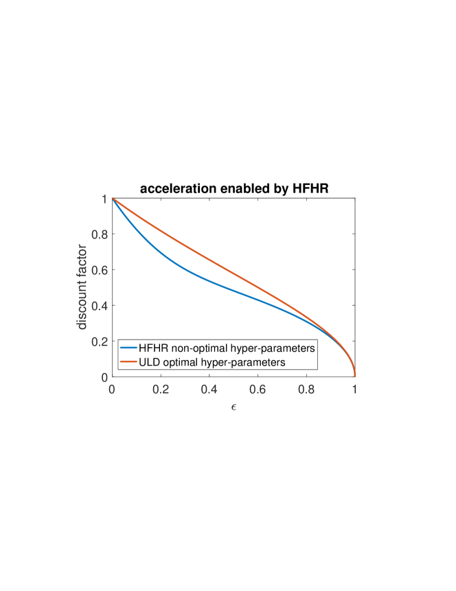
Figure 5: Acceleration of HFHR algorithm over ULD algorithm (despite of an additional constraint $\alpha$ may place on $h$) for multi-dimensional quadratic objectives. $1/\epsilon$ is the condition number.

The exact expressions of discount factors are also plotted in Fig.5 ($c=1$ was arbitrarily chosen) and one can see acceleration for any (not necessarily small) $\epsilon$.

(ii details) How were values in (25) chosen? Following the idea detailed in (i), we consider a case where $A_{1}$ eigenvalues are both real, $A_{2}$ eigenvalues are complex conjugates, and all their norms are equal. Note there are 3 more cases, namely real/real, complex/real, and complex/complex, but we do not optimize over all cases for simplicity — the real/complex case is enough for outperforming the optimal ULD.

This case leads to at least the following equations

$$\begin{cases}\text{tr}A_{1}&=0\\ \det A_{1}+\det A_{2}&=0\end{cases}$$ (29)

One can solve this system of equations to obtain $\alpha$ and $\gamma$ as functions of $h$. Following the idea of choosing $h$ small enough to resolve the stiffness of the ODE

$$\begin{cases}\dot{q}_{2}&=p_{2}-\alpha\epsilon^{-1}q_{2}\\ \dot{p}_{2}&=-\epsilon^{-1}q_{2}-\gamma p_{2}\end{cases},$$

pick $h=c\epsilon$. Then (29) gives

$$\gamma=\frac{\sqrt{4c^{2}\epsilon^{4}+8c^{2}\epsilon^{3}+4c^{2}\epsilon^{2}+\epsilon^{2}-2\epsilon+1}+\epsilon+3}{2c\epsilon^{2}+2c\epsilon}$$

$$\alpha=\frac{-\sqrt{4c^{2}\epsilon^{4}+8c^{2}\epsilon^{3}+4c^{2}\epsilon^{2}+\epsilon^{2}-2\epsilon+1}+3\epsilon+1}{2c\epsilon^{2}+2c\epsilon}$$

or

$$\gamma=\frac{-\sqrt{4c^{2}\epsilon^{4}+8c^{2}\epsilon^{3}+4c^{2}\epsilon^{2}+\epsilon^{2}-2\epsilon+1}+\epsilon+3}{2c\epsilon^{2}+2c\epsilon}$$

$$\alpha=\frac{\sqrt{4c^{2}\epsilon^{4}+8c^{2}\epsilon^{3}+4c^{2}\epsilon^{2}+\epsilon^{2}-2\epsilon+1}+3\epsilon+1}{2c\epsilon^{2}+2c\epsilon}$$

The former is our choice (25) because it can be checked that the latter leads to $\det A_{1}>0$ which violates the assumption of a pair of plus and minus real eigenvalues.

It is possible to find optimal $\alpha,\gamma,h$ for HFHR for the Gaussian cases. One has to minimize $\det A_{2}$ under the constraint $\det A_{2}>0$ in addition to (29). And then do similar calculations for the other 3 cases, and then finally the best among the 4 cases. Doing so however does not give enough insights to determine optimal hyperparameters for sampling general distributions.

Appendix F Randomized Midpoint Discretization of HFHR

F.1 The algorithm

HFHR is based on a continuous dynamics that adds HFHR corrections to the Underdamped Langevin Dynamics (ULD). It can be turned into a sampling algorithm via either a low-order time discretization (e.g., HFHR Algorithm 1) or a more accurate one. To complement the main text, this section demonstrates the latter, based on a powerful recent progress in discretizing ULD, known as Randomized Midpoint Algorithm (RMA) (Shen & Lee, 2019), and shows that the acceleration created by the HFHR correction terms persists.

More specifically, RMA is a high-order discretization scheme for ULD that achieved a better $\mathcal{O}(d^{\frac{1}{3}})$ dimension dependence of mixing time than first-order discretization of ULD, e.g., 1st-order KLMC (Dalalyan & Riou-Durand, 2020). Although RMA is originally designed specifically for ULD only, it is a general idea and already adapted to overdamped Langevin (He et al., 2020). Here we show it can be easily adapted to HFHR as well, as illustrated by the following Algorithm 2. Red highlights algorithmic changes we made to account for the HFHR corrections of ULD.

Algorithm 2 Randomized Midpoint Algorithm from (Shen & Lee, 2019), adapted for HFHR

1:  Input: potential function $f$ and its gradient $\nabla f$, damping coefficients $\alpha$ and $\gamma$, step size $h$, initial condition $(\boldsymbol{q}_{0},\boldsymbol{p}_{0})$

2:  procedure RMA-HFHR($f,\nabla f,\alpha,\gamma,h,\boldsymbol{q}_{0},\boldsymbol{p}_{0}$)

3:     $k=0$ and initialize $\begin{bmatrix}\boldsymbol{q}_{0}\\ \boldsymbol{p}_{0}\end{bmatrix}$

4:     while not converged do

5:        Generate an independent uniform random variable $\theta_{k}\sim U(0,1)$

6:        Generate Gaussian random vectors $\left(\boldsymbol{W}^{1}_{k+1},\boldsymbol{W}^{2}_{k+1},\boldsymbol{W}^{3}_{k+1}\right)\in\mathbb{R}^{3d}$ as in (Shen & Lee, 2019, Appendix A)

7:         Generate Gaussian random vectors $\boldsymbol{B}^{1}_{k+1},\boldsymbol{B}^{2}_{k+1}\in\mathbb{R}^{d}$ as described by (31)

8:        $\boldsymbol{q}_{k+\frac{1}{2}}=\boldsymbol{q}_{k}+\frac{1}{\gamma}(1-e^{-\gamma\theta_{k}h})\boldsymbol{p}_{k}-\frac{1}{\gamma}\left(\theta_{k}h-\frac{1}{\gamma}(1-e^{-\gamma\theta_{k}h})\right)\nabla f(\boldsymbol{q}_{k})+\boldsymbol{W}^{1}_{k+1}$ $\color[rgb]{1,0,0}-\alpha\theta_{k}h\nabla f(\boldsymbol{q}_{k})+\sqrt{2\alpha}\boldsymbol{B}^{1}_{k+1}$

9:        $\boldsymbol{q}_{k+1}=\boldsymbol{q}_{k}+\frac{1}{\gamma}(1-e^{-\gamma h})\boldsymbol{p}_{k}-\frac{1}{\gamma}h(1-e^{-\gamma(h-\theta_{k}h)})\nabla f(\boldsymbol{q}_{k+\frac{1}{2}})+\boldsymbol{W}^{2}_{k+1}\color[rgb]{1,0,0}-\alpha h\nabla f(\boldsymbol{q}_{k+\frac{1}{2}})+\sqrt{2\alpha}(\boldsymbol{B}^{1}_{k+1}+\boldsymbol{B}^{2}_{k+1})$

10:        $\boldsymbol{p}_{k+1}=\boldsymbol{p}_{k}e^{-\gamma h}-he^{-\gamma(h-\theta_{k}h)}\nabla f(\boldsymbol{q}_{k+\frac{1}{2}})+2\boldsymbol{W}^{3}_{k+1}$

11:        $k\leftarrow k+1$

12:     end while

13:  end procedure

The red parts basically correspond to two Euler-Maruyama time-steppings of an auxiliary dynamics that contains only the HFHR correction terms

$$d\boldsymbol{q}=-\alpha\nabla f(\boldsymbol{q})dt+\sqrt{2\alpha}d\boldsymbol{B}_{t},$$ (30)

first over a $\theta_{k}h$ timestep, and then over an $h$ timestep. These two steps originate from an operator splitting treatment of the full HFHR dynamics (eq.6), which is split into ULD and (30). Therefore, it is natural to see that

$$\boldsymbol{B}_{k+1}^{1}=\int_{hk}^{h(k+\theta_{k})}d\boldsymbol{B}_{t},\qquad\boldsymbol{B}_{k+1}^{2}=\int_{h(k+\theta_{k})}^{h(k+1)}d\boldsymbol{B}_{t},$$

and therefore $B_{k+1}^{1}$ and $B_{k+1}^{2}$ are, when conditioned on $\theta_{k}$, centered Gaussian vectors independent from each other and the $\boldsymbol{W}$’s, each being $d$-dimensional with i.i.d. entries, and they can be generated via

$$\boldsymbol{B}_{k+1}^{1}=\sqrt{\theta_{k}h}\boldsymbol{\xi}_{k+1}^{1},\qquad\boldsymbol{B}_{k+1}^{2}=\sqrt{h-\theta_{k}h}\boldsymbol{\xi}_{k+1}^{2},$$ (31)

where $\boldsymbol{\xi}_{k+1}^{1}$ and $\boldsymbol{\xi}_{k+1}^{2}$ are i.i.d. standard d-dimensional Gaussian vectors.

Remark F.1.

In the original RMA (Shen & Lee, 2019, Algorithm 1), the uniform random variable for the midpoint’s proportional location was denoted by $\alpha$. However, since we have already used this letter for the HFHR correction coefficient, we use instead $\theta$ to denote this uniform random variable.

Remark F.2.

From the red text, it is easy to see that if $\alpha=0$, Algorithm 2 degenerates to RMA for ULD. Nevertheless, Algorithm 2 is again just one RMA discretization of HFHR but not the only one.

F.2 Numerical results: HFHR again accelerates

To numerically compare the RMA discretization of HFHR dynamics and ULD dynamics (note we don’t compare 1st-order HFHR Algorithm 1 with RMA-ULD as we’d like to compare apple with apple), we conduct an experiment very similar to that in Sec.6.2, with the same nonlinear potential function. We run both RMA for ULD and RMA for HFHR with dimension $d=10$, initial value $(100\times\boldsymbol{1}_{d},\boldsymbol{0}_{d})$, $h=1$ (chosen to be near the stability limit of RMA-ULD), a family of $\gamma\in\{0.1,0.2,0.5,1,2,5,10,20,50,100\}$ and $\alpha\in\{$0, 0.001, 0.002, 0.005, 0.01, 0.02, 0.05, 0.1, 0.2, 0.5, 0.55, 0.6, 0.65,0.7,0.75,0.8,0.85,0.9,0.95, 1, 2, 5, 10, 20, 50, 100$\}$. For each algorithm and each set of parameter values, we run 1,000 independent realizations to compute statistics and estimate the mean time of reaching $\varepsilon=0.1$ neighborhood of the target distribution. Then, for each $\alpha$ (including $\alpha=0$, which is the original RMA), we optimize over $\gamma$ choices to get the best results. To further reduce variance, we also repeat the experiment with 100 different random seeds.

Too large $\alpha$ values with which Algorithm 2 fails to reach $\epsilon$-neighborhood are not plotted and the final results are shown in Figure 6. It clearly suggests that with appropriated chosen $\alpha$ ($\alpha=0.5$ in our case), RMA discretized HFHR dynamics requires fewer iterations than RMA discretized ULD, which suggests a better iteration complexity.

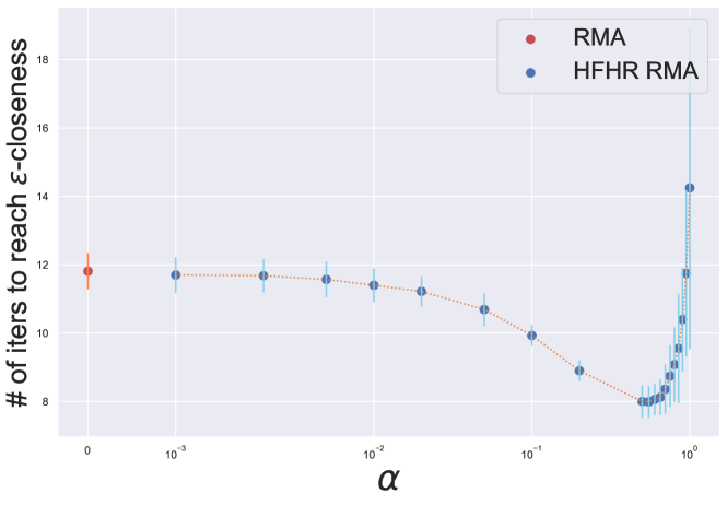
Figure 6: Improvement of RMA for HFHR (Algorithm 2) over the original RMA (for ULD) in iteration complexity. (vertical bar = 1 standard deviation)

References

• Alvarez et al. (2002) Alvarez, F., Attouch, H., Bolte, J., and Redont, P. A second-order gradient-like dissipative dynamical system with hessian-driven damping.: Application to optimization and mechanics. Journal de mathématiques pures et appliquées, 81(8):747–779, 2002.
• Attouch et al. (2018) Attouch, H., Chbani, Z., Peypouquet, J., and Redont, P. Fast convergence of inertial dynamics and algorithms with asymptotic vanishing viscosity. Mathematical Programming, 168(1-2):123–175, 2018.
• Attouch et al. (2020) Attouch, H., Chbani, Z., Fadili, J., and Riahi, H. First-order optimization algorithms via inertial systems with hessian driven damping. Mathematical Programming, pp.  1–43, 2020.
• Baudoin (2017) Baudoin, F. Bakry-emery meet villani. Journal of Functional Analysis, 2017.
• Bierkens et al. (2019) Bierkens, G., Fearnhead, P., and Roberts, G. The zig-zag process and super-efficient sampling for bayesian analysis of big data. Annals of Statistics, 47(3), 2019.
• Bouchard-Côté et al. (2018) Bouchard-Côté, A., Vollmer, S. J., and Doucet, A. The bouncy particle sampler: A nonreversible rejection-free markov chain monte carlo method. Journal of the American Statistical Association, 113(522):855–867, 2018.
• Bubeck et al. (2018) Bubeck, S., Eldan, R., and Lehec, J. Sampling from a log-concave distribution with projected langevin monte carlo. Discrete & Computational Geometry, 59(4):757–783, 2018.
• Cao et al. (2019) Cao, Y., Lu, J., and Wang, L. On explicit $l_{2}$-convergence rate estimate for underdamped langevin dynamics. arXiv preprint arXiv:1908.04746, 2019.
• Chen et al. (2015) Chen, C., Ding, N., and Carin, L. On the convergence of stochastic gradient MCMC algorithms with high-order integrators. NIPS, 2015.
• Chen et al. (2018a) Chen, C., Zhang, R., Wang, W., Li, B., and Chen, L. A unified particle-optimization framework for scalable bayesian sampling. In The Conference on Uncertainty in Artificial Intelligence, 2018a.
• Chen et al. (2018b) Chen, Y., Chen, J., Dong, J., Peng, J., and Wang, Z. Accelerating nonconvex learning via replica exchange langevin diffusion. In International Conference on Learning Representations, 2018b.
• Cheng & Bartlett (2018) Cheng, X. and Bartlett, P. L. Convergence of langevin mcmc in kl-divergence. PMLR 83, (83):186–211, 2018.
• Cheng et al. (2018) Cheng, X., Chatterji, N. S., Bartlett, P. L., and Jordan, M. I. Underdamped langevin mcmc: A non-asymptotic analysis. Proceedings of the 31st Conference On Learning Theory, PMLR, 2018.
• Chewi et al. (2021) Chewi, S., Lu, C., Ahn, K., Cheng, X., Gouic, T. L., and Rigollet, P. Optimal dimension dependence of the metropolis-adjusted langevin algorithm. COLT, 2021.
• Chizat & Bach (2018) Chizat, L. and Bach, F. On the global convergence of gradient descent for over-parameterized models using optimal transport. In Advances in neural information processing systems, pp. 3036–3046, 2018.
• Dalalyan (2017a) Dalalyan, A. Further and stronger analogy between sampling and optimization: Langevin monte carlo and gradient descent. In Conference on Learning Theory, pp.  678–689. PMLR, 2017a.
• Dalalyan (2017b) Dalalyan, A. S. Theoretical guarantees for approximate sampling from smooth and log-concave densities. Journal of the Royal Statistical Society: Series B (Statistical Methodology), 79(3):651–676, 2017b.
• Dalalyan & Riou-Durand (2020) Dalalyan, A. S. and Riou-Durand, L. On sampling from a log-concave density using kinetic Langevin diffusions. Bernoulli, 26(3):1956–1988, 2020.
• Deng et al. (2020) Deng, W., Feng, Q., Gao, L., Liang, F., and Lin, G. Non-convex learning via replica exchange stochastic gradient mcmc. In International Conference on Machine Learning, pp. 2474–2483. PMLR, 2020.
• Ding et al. (2021) Ding, Z., Li, Q., Lu, J., and Wright, S. Random coordinate underdamped langevin monte carlo. In International conference on artificial intelligence and statistics, pp.  2701–2709. PMLR, 2021.
• Dolbeault et al. (2009) Dolbeault, J., Mouhot, C., and Schmeiser, C. Hypocoercivity for kinetic equations with linear relaxation terms. Comptes Rendus Mathematique, 347(9-10):511–516, 2009.
• Dolbeault et al. (2015) Dolbeault, J., Mouhot, C., and Schmeiser, C. Hypocoercivity for linear kinetic equations conserving mass. Transactions of the American Mathematical Society, 367(6):3807–3828, 2015.
• Dua & Graff (2017) Dua, D. and Graff, C. UCI machine learning repository, 2017. URL http://archive.ics.uci.edu/ml.
• Duncan et al. (2016) Duncan, A. B., Lelievre, T., and Pavliotis, G. Variance reduction using nonreversible langevin samplers. Journal of statistical physics, 163(3):457–491, 2016.
• Durmus & Moulines (2016) Durmus, A. and Moulines, E. Sampling from strongly log-concave distributions with the unadjusted langevin algorithm. arXiv preprint arXiv:1605.01559, 5, 2016.
• Durmus & Moulines (2019) Durmus, A. and Moulines, E. High-dimensional bayesian inference via the unadjusted langevin algorithm. Bernoulli, 25(4A):2854–2882, 2019.
• Durmus et al. (2019) Durmus, A., Majewski, S., and Miasojedow, B. Analysis of langevin monte carlo via convex optimization. The Journal of Machine Learning Research, 20(1):2666–2711, 2019.
• Dwivedi et al. (2019) Dwivedi, R., Chen, Y., Wainwright, M. J., and Yu, B. Log-concave sampling: Metropolis-hastings algorithms are fast. Journal of Machine Learning Research, 20(183):1–42, 2019.
• Eberle et al. (2019) Eberle, A., Guillin, A., Zimmer, R., et al. Couplings and quantitative contraction rates for langevin dynamics. The Annals of Probability, 47(4):1982–2010, 2019.
• Eckmann & Hairer (2003) Eckmann, J.-P. and Hairer, M. Spectral properties of hypoelliptic operators. Communications in mathematical physics, 235(2):233–253, 2003.
• Erdogdu & Hosseinzadeh (2021) Erdogdu, M. A. and Hosseinzadeh, R. On the convergence of langevin monte carlo: The interplay between tail growth and smoothness. COLT, 2021.
• Frogner & Poggio (2020) Frogner, C. and Poggio, T. Approximate inference with wasserstein gradient flows. In International Conference on Artificial Intelligence and Statistics, 2020.
• He et al. (2020) He, Y., Balasubramanian, K., and Erdogdu, M. A. On the ergodicity, bias and asymptotic normality of randomized midpoint sampling method. Advances in Neural Information Processing Systems, 33, 2020.
• Hu & Lessard (2017) Hu, B. and Lessard, L. Dissipativity theory for nesterov’s accelerated method. In Proceedings of the 34th International Conference on Machine Learning-Volume 70, pp.  1549–1557. JMLR.org, 2017.
• Hwang et al. (2005) Hwang, C.-R., Hwang-Ma, S.-Y., Sheu, S.-J., et al. Accelerating diffusions. Annals of Applied Probability, 15(2):1433–1444, 2005.
• Jordan et al. (1998) Jordan, R., Kinderlehrer, D., and Otto, F. The variational formulation of the fokker–planck equation. SIAM journal on mathematical analysis, 29(1):1–17, 1998.
• Kim et al. (2016) Kim, A. K., Samworth, R. J., et al. Global rates of convergence in log-concave density estimation. The Annals of Statistics, 44(6):2756–2779, 2016.
• Kozlov (1989) Kozlov, S. M. Effective diffusion in the fokker-planck equation. Mathematical notes of the Academy of Sciences of the USSR, 45:360–368, 1989.
• Leimkuhler et al. (2018) Leimkuhler, B., Matthews, C., and Weare, J. Ensemble preconditioning for markov chain monte carlo simulation. Statistics and Computing, 28(2):277–290, 2018.
• Lelievre et al. (2013) Lelievre, T., Nier, F., and Pavliotis, G. A. Optimal non-reversible linear drift for the convergence to equilibrium of a diffusion. Journal of Statistical Physics, 152(2):237–274, 2013.
• Li et al. (2022a) Li, R., Tao, M., Vempala, S. S., and Wibisono, A. The mirror langevin algorithm converges with vanishing bias. In International Conference on Algorithmic Learning Theory, pp.  718–742. PMLR, 2022a.
• Li et al. (2022b) Li, R., Zha, H., and Tao, M. Sqrt (d) dimension dependence of langevin monte carlo. ICLR, 2022b.
• Li et al. (2019) Li, X., Wu, D., Mackey, L., and Erdogdu, M. A. Stochastic Runge-Kutta accelerates Langevin Monte Carlo and beyond. NeurIPS, 2019.
• Liang & Chen (2022) Liang, J. and Chen, Y. A proximal algorithm for sampling from non-convex potentials. preprint arXiv:2205.10188, 2022.
• Liu et al. (2019) Liu, C., Zhuo, J., Cheng, P., Zhang, R., and Zhu, J. Understanding and accelerating particle-based variational inference. In International Conference on Machine Learning, pp. 4082–4092, 2019.
• Liu & Wang (2016) Liu, Q. and Wang, D. Stein variational gradient descent: A general purpose bayesian inference algorithm. In Advances in neural information processing systems, pp. 2378–2386, 2016.
• Ma et al. (2019) Ma, Y.-A., Chen, Y., Jin, C., Flammarion, N., and Jordan, M. I. Sampling can be faster than optimization. Proceedings of the National Academy of Sciences, 116(42):20881–20885, 2019.
• Ma et al. (2021) Ma, Y.-A., Chatterji, N., Cheng, X., Flammarion, N., Bartlett, P., and Jordan, M. I. Is there an analog of nesterov acceleration for mcmc? Bernoulli, 2021.
• Mattingly et al. (2002) Mattingly, J. C., Stuart, A. M., and Higham, D. J. Ergodicity for sdes and approximations: locally lipschitz vector fields and degenerate noise. Stochastic processes and their applications, 101(2):185–232, 2002.
• McLachlan & Quispel (2002) McLachlan, R. I. and Quispel, G. R. W. Splitting methods. Acta Numerica, 11:341, 2002.
• Meyn et al. (1994) Meyn, S. P., Tweedie, R. L., et al. Computable bounds for geometric convergence rates of markov chains. The Annals of Applied Probability, 4(4):981–1011, 1994.
• Nesterov (1983) Nesterov, Y. A method for unconstrained convex minimization problem with the rate of convergence o (1/k^ 2). In Doklady AN USSR, volume 269, pp.  543–547, 1983.
• Nesterov (2013) Nesterov, Y. Introductory lectures on convex optimization: A basic course, volume 87. Springer Science & Business Media, 2013.
• Ohzeki & Ichiki (2015) Ohzeki, M. and Ichiki, A. Langevin dynamics neglecting detailed balance condition. Physical Review E, 92(1):012105, 2015.
• Pavliotis (2014) Pavliotis, G. A. Stochastic processes and applications: diffusion processes, the Fokker-Planck and Langevin equations, volume 60. Springer, 2014.
• Polyak (1964) Polyak, B. T. Some methods of speeding up the convergence of iteration methods. USSR Computational Mathematics and Mathematical Physics, 4(5):1–17, 1964.
• Rey-Bellet & Spiliopoulos (2015) Rey-Bellet, L. and Spiliopoulos, K. Irreversible langevin samplers and variance reduction: a large deviations approach. Nonlinearity, 28(7):2081, 2015.
• Roberts et al. (1996) Roberts, G. O., Tweedie, R. L., et al. Exponential convergence of langevin distributions and their discrete approximations. Bernoulli, 2(4):341–363, 1996.
• Roussel & Stoltz (2018) Roussel, J. and Stoltz, G. Spectral methods for langevin dynamics and associated error estimates. ESAIM: Mathematical Modelling and Numerical Analysis, 52(3):1051–1083, 2018.
• Shen & Lee (2019) Shen, R. and Lee, Y. T. The randomized midpoint method for log-concave sampling. In Advances in Neural Information Processing Systems, pp. 2098–2109, 2019.
• Shi et al. (2021) Shi, B., Du, S. S., Jordan, M. I., and Su, W. J. Understanding the acceleration phenomenon via high-resolution differential equations. Mathematical Programming, pp.  1–70, 2021.
• Souza & Tao (2019) Souza, A. N. and Tao, M. Metastable transitions in inertial langevin systems: What can be different from the overdamped case? European Journal of Applied Mathematics, 30(5):830–852, 2019.
• Strang (1968) Strang, G. On the construction and comparison of difference schemes. SIAM journal on numerical analysis, 5(3):506–517, 1968.
• Su et al. (2014) Su, W., Boyd, S., and Candes, E. A differential equation for modeling nesterov’s accelerated gradient method: Theory and insights. In Advances in Neural Information Processing Systems, pp. 2510–2518, 2014.
• Taghvaei & Mehta (2019) Taghvaei, A. and Mehta, P. Accelerated flow for probability distributions. In Chaudhuri, K. and Salakhutdinov, R. (eds.), Proceedings of the 36th International Conference on Machine Learning, volume 97 of Proceedings of Machine Learning Research, pp.  6076–6085, Long Beach, California, USA, 09–15 Jun 2019. PMLR.
• Trotter (1959) Trotter, H. F. Product of semigroups of operators. Proc. Amer. Math. Soc., 10:545–551, 1959.
• Vempala & Wibisono (2019) Vempala, S. and Wibisono, A. Rapid convergence of the unadjusted langevin algorithm: Isoperimetry suffices. In Advances in Neural Information Processing Systems, pp. 8092–8104, 2019.
• Villani (2008) Villani, C. Optimal transport: old and new, volume 338. Springer Science & Business Media, 2008.
• Villani (2009) Villani, C. Hypocoercivity. Memoirs of the American Mathematical Society, 202(950), 2009.
• Wang & Li (2019) Wang, Y. and Li, W. Accelerated information gradient flow. arXiv preprint arXiv:1909.02102, 2019.
• Wibisono (2018) Wibisono, A. Sampling as optimization in the space of measures: The langevin dynamics as a composite optimization problem. In Conference On Learning Theory, pp.  2093–3027, 2018.
• Wibisono et al. (2016) Wibisono, A., Wilson, A. C., and Jordan, M. I. A variational perspective on accelerated methods in optimization. Proceedings of the National Academy of Sciences, 113(47):E7351–E7358, 2016.
• Wilson et al. (2021) Wilson, A. C., Recht, B., and Jordan, M. I. A lyapunov analysis of accelerated methods in optimization. Journal of Machine Learning Research, 22(113):1–34, 2021.
• Wilson (2020) Wilson, A. G. The case for bayesian deep learning. arXiv preprint arXiv:2001.10995, 2020.
• Zhang et al. (2018) Zhang, R., Chen, C., Li, C., and Carin, L. Policy optimization as wasserstein gradient flows. In International Conference on Machine Learning, pp. 5737–5746, 2018.