MS-TCN++: Multi-Stage Temporal Convolutional Network for Action Segmentation

Abstract

With the success of deep learning in classifying short trimmed videos, more attention has been focused on temporally segmenting and classifying activities in long untrimmed videos. State-of-the-art approaches for action segmentation utilize several layers of temporal convolution and temporal pooling. Despite the capabilities of these approaches in capturing temporal dependencies, their predictions suffer from over-segmentation errors. In this paper, we propose a multi-stage architecture for the temporal action segmentation task that overcomes the limitations of the previous approaches. The first stage generates an initial prediction that is refined by the next ones. In each stage we stack several layers of dilated temporal convolutions covering a large receptive field with few parameters. While this architecture already performs well, lower layers still suffer from a small receptive field. To address this limitation, we propose a dual dilated layer that combines both large and small receptive fields. We further decouple the design of the first stage from the refining stages to address the different requirements of these stages. Extensive evaluation shows the effectiveness of the proposed model in capturing long-range dependencies and recognizing action segments. Our models achieve state-of-the-art results on three datasets: 50Salads, Georgia Tech Egocentric Activities (GTEA), and the Breakfast dataset.

1 Introduction

Action recognition from video has been an active research area in computer vision in the past few years. Most of the efforts, however, have been focused on classifying short trimmed videos [1, 2, 3, 4]. Despite the success of these approaches on trimmed videos with a single activity, their performance is limited on long videos containing many action segments. Since for many applications, like surveillance and robotics, it is crucial to temporally segment activities in long untrimmed videos, approaches for temporal action segmentation have received more attention. Early attempts for temporal action segmentation tried to extend the success on trimmed videos by combining these models with sliding windows [5, 6, 7]. These approaches use temporal windows of different scales to detect and classify action segments. However, such approaches are expensive and do not scale for long videos. Other approaches apply a coarse temporal modeling using Markov models on top of frame-wise classifiers [8, 9, 10]. While these approaches achieved good results, they are very slow as they require solving a maximization problem over very long sequences.

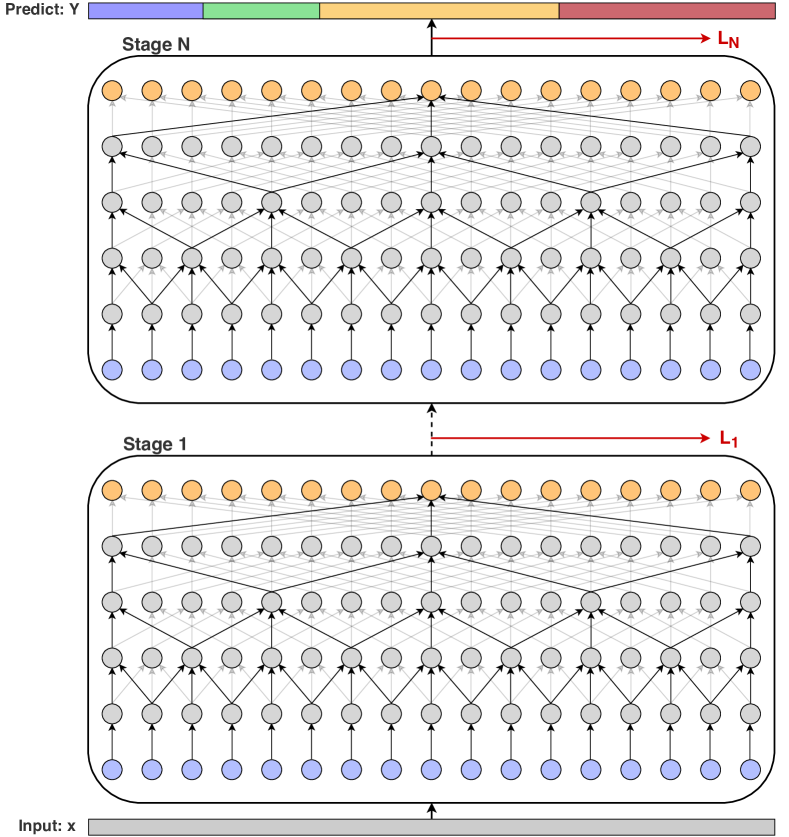
Figure 1: Overview of the multi-stage temporal convolutional network. Each stage generates an initial prediction that is refined by the next stage. At each stage, several dilated 1D convolutions are applied on the activations of the previous layer. A loss layer is added after each stage.

With the success of temporal convolutional networks (TCNs) as a powerful temporal model for speech synthesis, many researchers adapt TCN-based models for the temporal action segmentation task [11, 12, 13]. These models were more capable in capturing long range dependencies between the video frames by relying on a large receptive field. However, these models are limited for a very low temporal resolution of a few frames per second. Furthermore, since these approaches rely on temporal pooling layers to increase the receptive field, many of the fine-grained information that is necessary for recognition is lost.

To overcome the limitations of the previous approaches, we propose a new model that also uses temporal convolutions. In contrast to previous approaches, the proposed model operates on the full temporal resolution of the videos and thus achieves better results. Our model consists of multiple stages where each stage outputs an initial prediction that is refined by the next one. We call the new architecture Multi-Stage Temporal Convolutional Network (MS-TCN). In each stage, we apply a series of dilated 1D convolutions, which enables the model to have a large temporal receptive field with less parameters. Figure 1 shows an overview of the proposed multi-stage model. Furthermore, we employ a smoothing loss during training which penalizes over-segmentation errors in the predictions.

A preliminary version of this work introducing MS-TCN and the smoothing loss has been published in [14]. While the proposed MS-TCN already achieves good performance, some of the design choices are sub-optimal. First, while the receptive field is very large for higher layers in MS-TCN, lower layers suffer from a small receptive field. Second, the first stage in MS-TCN generates an initial prediction and the remaining stages refine this prediction. Despite the differences between these two tasks, all stages share the same architecture. To address the first limitation, we propose a dual dilated layer (DDL) which combines both large and small receptive fields at each layer. For the second, we divide the whole architecture into two parts: The first part is the first stage, which is the prediction generation stage, and the second part consists of prediction refinement stages. Then we customize the architecture of each part separately and do not force all stages to have the same architecture as in MS-TCN. By incorporating these design choices on MS-TCN, we propose an improved version of the model, which we call MS-TCN++. Furthermore, we show that the parameters of the refinement stages in MS-TCN++ can be shared without compromising the accuracy. This model achieves superior performance compared to MS-TCN with much less parameters. Our contribution beyond [14] is thus three folded:

• We propose a dual dilated layer that combines large and small receptive fields.

• We optimize the architecture design of MS-TCN by decoupling the prediction phase and the refinement phase. We call the new model MS-TCN++, which achieves superior results compared to MS-TCN.

• We further show that sharing the parameters between the refinement stages in MS-TCN++ results in a more compact model without compromising performance.

Extensive evaluation shows the effectiveness of our models in capturing long range dependencies between action classes and producing high quality predictions. Our approach achieves state-of-the-art results on three challenging benchmarks for action segmentation: 50Salads [15], Georgia Tech Egocentric Activities (GTEA) [16], and the Breakfast dataset [17]. Moreover, the proposed models are view-agnostic and work well on all the three datasets, which depict videos with third person view, top view and egocentric videos.

2 Related Work

Temporal action segmentation has received a lot of interest from the computer vision community. Many approaches where proposed to localize action segments in videos or assign action labels to video frames. In earlier approaches, a sliding window approach is applied with non-maximum suppression [5, 6]. However, such approaches are computationally expensive since the model has to be evaluated at different window scales. Other approaches model actions based on the change in the state of objects and materials [18] or based on the interactions between hands and objects [19]. Bhattacharya et al. [20] use a vector time series representation of videos to model the temporal dynamics of complex actions using methods from linear dynamical systems theory. The representation is based on the output of pre-trained concept detectors applied on overlapping temporal windows. Cheng et al. [21] represent videos as a sequence of visual words, and model the temporal dependency by employing a Bayesian non-parametric model of discrete sequences to jointly classify and segment video sequences.

Despite the success of the previous approaches, their performance was limited as they failed in capturing the context over long video sequences. To alleviate this problem, many proposals tried to employ high level temporal modeling over frame-wise classifiers. Kuehne et al. [8] represent the frames of a video using Fisher vectors of improved dense trajectories, and then each action is modeled with a hidden Markov model (HMM). These HMMs are combined with a context-free grammar for recognition to determine the most probable sequence of actions. HMMs are also used in many other approaches. [22] combine HMMs with a Gaussian mixture model (GMM) as a frame-wise classifier. However, since frame-wise classifiers do not capture enough context to detect action classes, Richard et al. [10] and Kuehne et al. [23] use a GRU instead of the GMM that is used in [22]. A hidden Markov model is also used in [24] to model both transitions between states and their durations. Vo and Bobick [25] use a Bayes network to segment activities. They represent compositions of actions using a stochastic context-free grammar with AND-OR operations. [26] propose a model for temporal action detection that consists of three components: an action model that maps features extracted from the video frames into action probabilities, a language model that describes the probability of actions at sequence level, and finally a length model that models the length of different action segments. To get the video segmentation, they use dynamic programming to find the solution that maximizes the joint probability of the three models. Singh et al. [27] use a two-stream network to learn representations of short video chunks. These representations are then passed to a bi-directional LSTM to capture dependencies between different chunks. However, their approach is very slow due to the sequential prediction. In [28], a three-stream architecture that operates on spatial, temporal and egocentric streams is introduced to learn egocentric-specific features. These features are then classified using a multi-class SVM.

Multi-scale information is important for speech synthesis [29] and image recognition [30]. Inspired by these, researchers have tried to use similar ideas for the temporal action segmentation task. Lea et al. [11] propose a temporal convolutional network for action segmentation and detection. Their approach follows an encoder-decoder architecture with a temporal convolution and pooling in the encoder, and upsampling followed by deconvolution in the decoder. While using temporal pooling enables the model to capture long-range dependencies, it might result in a loss of fine-grained information that is necessary for fine-grained recognition. Lei and Todorovic [12] build on top of [11] and use deformable convolutions instead of the normal convolution and add a residual stream to the encoder-decoder model. Ding and Xu [13] add lateral connections to the encoder-decoder TCN [11] and propose a temporal convolutional feature pyramid network for predicting frame-wise action labels. All of the approaches in [11, 12, 13] operate on downsampled videos with a temporal resolution of 1-3 frames per second. In contrast to these approaches, we operate on the full temporal resolution and use dilated convolutions to capture long-range dependencies. Recently, Mac et al. [31] propose to learn spatio-temporal features using deformable convolutions and local consistency constraints. On the contrary, in our approach we only focus on the long-term temporal modeling.

Action detection is a related but a different task. In this context, the goal is to detect sparse action segments while most parts of the videos are unlabeled. In this work, we focus on action segmentation where the videos are densely annotated. For action detection, several approaches follow a two stage pipeline. The first stage is to generate proposals, and then classify and refine the boundaries of these proposals in the second stage [32, 33, 34, 35, 36, 37, 38, 39, 40]. Other approaches combine the proposal generation and classification in a single-stage architecture which enables end-to-end training [41, 42, 43].

3 Temporal Action Segmentation

We introduce a multi-stage temporal convolutional network (MS-TCN) for the temporal action segmentation task. Then we introduce a new layer and address the limitations of MS-TCN to propose an improved model called MS-TCN++. Given the frames of a video $x_{1:T}=(x_{1},\dots,x_{T})$, our goal is to infer the class label for each frame $c_{1:T}=(c_{1},\dots,c_{T})$, where $T$ is the video length. First, we describe the single-stage approach in Section 3.1, then we discuss the multi-stage model in Section 3.2. Section 3.3 introduces the dual dilated layer. In Section 3.4, we analyze the drawbacks of MS-TCN and introduce the improved model MS-TCN++. Finally, we describe the proposed loss function in Section 3.5.

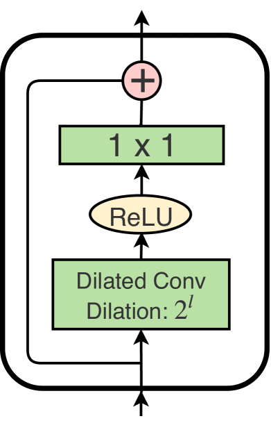
Figure 2: Overview of the dilated residual layer. At each layer $l$, the dilated residual layer uses a convolution with dilated factor $2^{l}$.

3.1 Single-Stage TCN

Our single stage model consists of only temporal convolutional layers. We do not use pooling layers, which reduce the temporal resolution, or fully connected layers, which force the model to operate on inputs of fixed size and massively increase the number of parameters. We call this model a single-stage temporal convolutional network (SS-TCN). The first layer of a single-stage TCN is a $1\times 1$ convolutional layer, that adjusts the dimension of the input features to match the number of feature maps in the network. Then, this layer is followed by several layers of dilated 1D convolution. Inspired by the wavenet [29] architecture, we use a dilation factor that is doubled at each layer, i.e. $1,2,4,....,512$. All these layers have the same number of convolutional filters. However, instead of the causal convolution that is used in wavenet, we use acausal convolutions with kernel size 3. Each layer applies a dilated convolution with ReLU activation to the output of the previous layer. We further use residual connections to facilitate gradients flow. The set of operations at each layer can be formally described as follows

$$\hat{H}_{l}=ReLU(W_{d}*H_{l-1}+b_{d}),$$ (1)

$$H_{l}=H_{l-1}+W*\hat{H}_{l}+b,$$ (2)

where $H_{l}$ is the output of layer $l$, $*$ denotes the convolution operator, $W_{d}\in\mathbb{R}^{3\times D\times D}$ are the weights of the dilated convolution filters with kernel size 3 and $D$ is the number of convolutional filters, $W\in\mathbb{R}^{1\times D\times D}$ are the weights of a $1\times 1$ convolution, and $b_{d},b\in\mathbb{R}^{D}$ are bias vectors. These operations are illustrated in Figure 2. Using dilated convolution increases the receptive field without the need to increase the number of parameters by increasing the number of layers or the kernel size. Since the receptive field grows exponentially with the number of layers, we can achieve a very large receptive field with a few layers, which helps in preventing the model from over-fitting the training data. The receptive field at each layer is determined by

$$ReceptiveField(l)=2^{l+1}-1,$$ (3)

where $l\in\left[1,L\right]$ is the layer number. Note that this formula is only valid for a kernel of size 3. To get the probabilities for the output class, we apply a $1\times 1$ convolution over the output of the last dilated convolution layer followed by a softmax activation, i.e.

$$Y_{t}=Softmax(Wh_{L,t}+b),$$ (4)

where $Y_{t}$ contains the class probabilities at time $t$, $h_{L,t}$ is the output of the last dilated convolution layer at time $t$, $W\in\mathbb{R}^{C\times D}$ and $b\in\mathbb{R}^{C}$ are the weights and bias for the $1\times 1$ convolution layer. $C$ is the number of classes and $D$ is the number of convolutional filters.

3.2 Multi-Stage TCN

Stacking several predictors sequentially has shown significant improvements in many tasks like human pose estimation [44, 45, 46]. The idea of these stacked or multi-stage architectures is composing several models sequentially such that each model operates directly on the output of the previous one. The effect of such composition is an incremental refinement of the predictions from the previous stages.

Motivated by the success of such architectures, we introduce a multi-stage temporal convolutional network (MS-TCN) for the temporal action segmentation task. In this multi-stage model, each stage takes an initial prediction from the previous stage and refines it. The input of the first stage are the frame-wise features of the video as follows

$$Y^{0}=x_{1:T},$$ (5)

$$Y^{s}=\mathcal{F}(Y^{s-1}),$$ (6)

where $Y^{s}$ is the output at stage $s$ and $\mathcal{F}$ is the single-stage TCN discussed in Section 3.1. Using such a multi-stage architecture helps in providing more context to predict the class label at each frame. Furthermore, since the output of each stage is an initial prediction, the network is able to capture dependencies between action classes and learn plausible action sequences, which helps in reducing the over-segmentation errors.

Note that the input to the next stage is just the frame-wise probabilities without any additional features. We will show in the experiments how adding features to the input of the next stage affects the quality of the predictions.

3.3 Dual Dilated Layer

In the dilated convolution layers in MS-TCN, the dilation factor increases as we increase the number of layers. While this results in a large receptive field for higher layers, lower layers still suffer from very low receptive fields. Furthermore, higher layers in MS-TCN apply convolutions over very distant time steps due to the large dilation factor. To overcome this problem, we propose a dual dilated layer (DDL). Instead of having one dilated convolution, the DDL combines two convolutions with different dilation factor. The first convolution has a low dilation factor in lower layers and exponentially increases as we increases the number of layers. Whereas for the second convolution, we start with a large dilation factor in lower layers and exponentially decrease it with increasing the number of layers. The set of operations at each layer can be formally described as follows

$$\hat{H}_{l,d_{1}}=W_{d_{1}}*H_{l-1}+b_{d_{1}},$$ (7)

$$\hat{H}_{l,d_{2}}=W_{d_{2}}*H_{l-1}+b_{d_{2}},$$ (8)

$$\hat{H}_{l}=ReLU([\hat{H}_{l,d_{1}},\hat{H}_{l,d_{2}}]),$$ (9)

$$H_{l}=H_{l-1}+W*\hat{H}_{l}+b,$$ (10)

where $W_{d_{1}},W_{d_{2}}\in\mathbb{R}^{3\times D\times D}$ are the weights of dilated convolutions with dilation factor $2^{l}$ and $2^{L-l}$ respectively, $W\in\mathbb{R}^{1\times 2D\times D}$ are the weights of a $1\times 1$ convolution, and $b_{d_{1}},b_{d_{2}},b\in\mathbb{R}^{D}$ are bias vectors. In (9), $\hat{H}_{l,d_{1}}$ and $\hat{H}_{l,d_{2}}$ are concatenated. An overview of the dual dilated layer is illustrated in Figure 3.

While the dual dilated layer combines local and global context from the input sequence, there are other techniques in the literature for fusing multi-scale features like feature pyramid networks (FPN) [47]. While applying FPN for temporal action segmentation has been successful [13], these approaches still suffer from a very limited receptive field. Moreover, the multi-scale features in FPN are obtained by applying pooling operations which results in a loss of the fine-grained information that is necessary for temporal segmentation. On the contrary, DDL combines multi-scale features and yet preserves the temporal resolution of the input sequence.

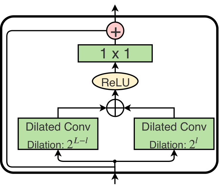
Figure 3: Overview of the dual dilated layer (DDL). At each layer $l$, DDL uses two convolutions with dilated factor $2^{l}$ and $2^{L-l}$, respectively, where $L$ is the number of layers in the network.

3.4 MS-TCN++

In this section, we introduce MS-TCN++, which utilizes the proposed dual dilated layer to improve MS-TCN. Similar to MS-TCN, the first stage in MS-TCN++ is responsible for generating the initial prediction, whereas the remaining stages incrementally refine this prediction. For the prediction generation stage, we adapt an SS-TCN with dual dilated layers (Figure 3) replacing the simple dilated residual layers (Figure 2) that are originally used in SS-TCN. Using the DDL enables the prediction generation stage to capture both local and global features in all layers, which results in better predictions. As refinement is easier than prediction generation, we adapt the SS-TCN architecture with dilated residual layers for the refinement stages. In our experiments, we show that using DDL only for the first stage performs best. Figure 4 shows an overview of the proposed MS-TCN++.

While adding more stages incrementally refines the predictions, it also drastically increases the number of parameters. Nevertheless, as the refinement stages are sharing the same role, their parameters can be shared to get a more compact model. In the experiments, we show that sharing the parameters between the refinement stages significantly reduces the number of parameters with only a slight degradation in accuracy.

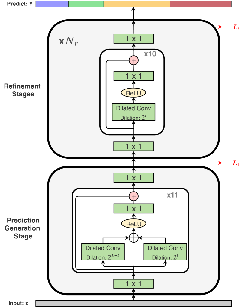
Figure 4: Overview of MS-TCN++. The first stage adapts an SS-TCN model with dual dilated layers. This stage generates an initial prediction that is refined incrementally by a set of $N_{r}$ refinement stages. For the refinement stages, an SS-TCN with dilated residual layers is used. A loss layer is added after each stage.

3.5 Loss Function

As a loss function, we use a combination of a classification loss and a smoothing loss. For the classification loss, we use a cross entropy loss

$$\mathcal{L}_{cls}=\frac{1}{T}\sum_{t}-log(y_{t,c}),$$ (11)

where $y_{t,c}$ is the predicted probability for the ground truth label $c$ at time $t$.

While the cross entropy loss already performs well, we found that the predictions for some of the videos contain a few over-segmentation errors. To further improve the quality of the predictions, we use an additional smoothing loss to reduce such over-segmentation errors. For this loss, we use a truncated mean squared error over the frame-wise log-probabilities

$$\mathcal{L}_{T-MSE}=\frac{1}{TC}\sum_{t,c}\tilde{\Delta}_{t,c}^{2},$$ (12)

$$\tilde{\Delta}_{t,c}=\begin{cases}\Delta_{t,c}&:\Delta_{t,c}\leq\tau\\ \tau&:otherwise\\ \end{cases},$$ (13)

$$\Delta_{t,c}=\left|log\ y_{t,c}-log\ y_{t-1,c}\right|,$$ (14)

where $T$ is the video length, $C$ is the number of classes, and $y_{t,c}$ is the probability of class $c$ at time $t$.

Note that the gradients are only computed with respect to $y_{t,c}$, whereas $y_{t-1,c}$ is not considered as a function of the model’s parameters. This loss is similar to the Kullback-Leibler (KL) divergence loss where

$$\mathcal{L}_{KL}=\frac{1}{T}\sum_{t,c}y_{t-1,c}(log\ y_{t-1,c}-log\ y_{t,c}).$$ (15)

However, we found that the truncated mean squared error ($\mathcal{L}_{T-MSE}$) (12) reduces the over-segmentation errors more. We will compare the KL loss and the proposed loss in the experiments.

The final loss function for a single stage is a combination of the above mentioned losses

$$\mathcal{L}_{s}=\mathcal{L}_{cls}+\lambda\mathcal{L}_{T-MSE},$$ (16)

where $\lambda$ is a model hyper-parameter to determine the contribution of the different losses. Finally to train the complete model, we minimize the sum of the losses over all stages

$$\mathcal{L}=\sum_{s}\mathcal{L}_{s}.$$ (17)

3.6 Implementation Details

For both MS-TCN and MS-TCN++, we use a multi-stage architecture with four stages. While all stages are the same for MS-TCN, the stages in MS-TCN++ consist of one prediction generation stage and three refinement stages. Each stage in MS-TCN and the refinement stages in MS-TCN++ contain ten dilated convolution layers. For the prediction generation stage in MS-TCN++, we use eleven layers. Dropout is used after each layer with probability $0.5$. We set the number of filters to $64$ in all layers of the model and the filter size is $3$. For the loss function, we set $\tau=4$ and $\lambda=0.15$. In all experiments, we use Adam optimizer with a learning rate of $0.0005$.

4 Experiments

Datasets. We evaluate the proposed models on three challenging datasets: 50Salads [15], Georgia Tech Egocentric Activities (GTEA) [16], and the Breakfast dataset [17]. Table I shows a summary of these datasets.

	# videos	# action classes	view	description
50Salads	50	17	top-view	salad preparation activities
GTEA	28	11	egocentric	7 different activities, like preparing coffee or cheese sandwich
Breakfast	1712	48	third person view	breakfast preparation related activities in 18 different kitchens

TABLE I: Summary of the used datasets in the experiments.

The 50Salads dataset contains 50 videos with $17$ action classes. The videos were recorded from the top view. On average, each video contains 20 action instances and is $6.4$ minutes long. As the name of the dataset indicates, the videos depict salad preparation activities. These activities were performed by $25$ actors where each actor prepared two different salads. For evaluation, we use five-fold cross-validation and report the average as in [15].

The GTEA dataset contains $28$ videos corresponding to 7 different activities, like preparing coffee or cheese sandwich, performed by 4 subjects. This dataset contains egocentric videos recorded by a camera that is mounted on the actor’s head. The frames of the videos are annotated with $11$ action classes including background. On average, each video has 20 action instances. We use cross-validation for evaluation by leaving one subject out.

The Breakfast dataset is the largest among the three datasets with $1,712$ third person view videos. The videos were recorded in 18 different kitchens showing breakfast preparation related activities. Overall, there are $48$ different actions where each video contains $6$ action instances on average. For evaluation, we use the standard 4 splits as proposed in [17] and report the average.

For all datasets, we extract I3D [3] features for the video frames and use these features as input to our model. For the GTEA and Breakfast datasets we use the temporal video resolution at $15$ fps, while for 50Salads we downsampled the features from $30$ fps to $15$ fps to be consistent with the other datasets.

Evaluation Metrics. For evaluation, we report the frame-wise accuracy (Acc), segmental edit distance and the segmental F1 score at overlapping thresholds $10\%,\ 25\%$ and $50\%$, denoted by $F1$@$\{10,25,50\}$. The overlapping threshold is determined based on the intersection over union (IoU) ratio. While the frame-wise accuracy is the most commonly used metric for action segmentation, long action classes have a higher impact than short action classes on this metric and over-segmentation errors have a very low impact. For that reason, we use the segmental F1 score as a measure of the quality of the prediction as proposed by [11].

4.1 Effect of the Number of Stages

We start our evaluation by showing the effect of using a multi-stage architecture (MS-TCN). Table II shows the results of a single-stage model compared to multi-stage models with different number of stages. As shown in the table, all of these models achieve a comparable frame-wise accuracy. Nevertheless, the quality of the predictions is very different. Looking at the segmental edit distance and F1 scores of these models, we can see that the single-stage model produces a lot of over-segmentation errors, as indicated by the low F1 score. On the other hand, using a multi-stage architecture reduces these errors and increases the F1 score. This effect is clearly visible when we use two or three stages, which gives a huge boost to the accuracy. Adding the fourth stage still improves the results but not as significant as the previous stages. However, by adding the fifth stage, we can see that the performance starts to degrade. This might be an over-fitting problem as a result of increasing the number of parameters. The effect of the multi-stage architecture can also be seen in the qualitative results shown in Figure 5. Adding more stages results in an incremental refinement of the predictions. In the rest of the experiments we use a multi-stage TCN with four stages.

	F1@{10,25,50}			Edit	Acc
SS-TCN	27.0	25.3	21.5	20.5	78.2
MS-TCN (2 stages)	55.5	52.9	47.3	47.9	79.8
MS-TCN (3 stages)	71.5	68.6	61.1	64.0	78.6
MS-TCN (4 stages)	76.3	74.0	64.5	67.9	80.7
MS-TCN (5 stages)	76.4	73.4	63.6	69.2	79.5

TABLE II: Effect of the number of stages on the 50Salads dataset.

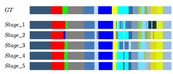
Figure 5: Qualitative result from the 50Salads dataset for comparing different number of stages.

4.2 Multi-Stage TCN vs. Deeper Single-Stage TCN

In the previous section, we have seen that our multi-stage architecture is better than a single-stage one. However, that comparison does not show whether the improvement is because of the multi-stage architecture or due to the increase in the number of parameters when adding more stages. For a fair comparison, we train a single-stage model that has the same number of parameters as the multi-stage one. As each stage in our MS-TCN contains $12$ layers (ten dilated convolutional layers, one $1\times 1$ convolutional layer and a softmax layer), we train a single-stage TCN with $48$ layers, which is the number of layers in a MS-TCN with four stages. For the dilated convolutions, we use similar dilation factors as in our MS-TCN. I.e. we start with a dilation factor of $1$ and double it at every layer up to a factor of $512$, and then we start again from $1$. As shown in Table III, our multi-stage architecture outperforms its single-stage counterpart with a large margin of up to $27\%$. This highlights the impact of the multi-stage architecture in improving the quality of the predictions.

	F1@{10,25,50}			Edit	Acc
SS-TCN (48 layers)	49.0	46.4	40.2	40.7	78.0
MS-TCN	76.3	74.0	64.5	67.9	80.7

TABLE III: Comparing a multi-stage TCN with a deep single-stage TCN on the 50Salads dataset.

4.3 Comparing Different Loss Functions

	F1@{10,25,50}			Edit	Acc
$\mathcal{L}_{cls}$	71.3	69.7	60.7	64.2	79.9
$\mathcal{L}_{cls}+\lambda\mathcal{L}_{KL}$	71.9	69.3	60.1	64.6	80.2
$\mathcal{L}_{cls}+\lambda\mathcal{L}_{T-MSE}$	76.3	74.0	64.5	67.9	80.7

TABLE IV: Comparing different loss functions on the 50Salads dataset.

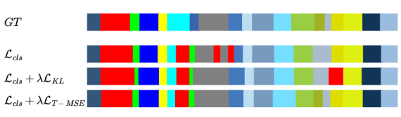
Figure 6: Qualitative result from the 50Salads dataset for comparing different loss functions.

As a loss function, we use a combination of a cross-entropy loss, which is common practice for classification tasks, and a truncated mean squared loss over the frame-wise log-probabilities to ensure smooth predictions. While the smoothing loss slightly improves the frame-wise accuracy compared to the cross entropy loss alone, we found that this loss produces much less over-segmentation errors. Table IV and Figure 6 show a comparison of these losses. As shown in Table IV, the proposed loss achieves better F1 and edit scores with an absolute improvement of up to $5\%$. This indicates that our loss produces less over-segmentation errors compared to cross entropy since it forces consecutive frames to have similar class probabilities, which results in a smoother output.

Penalizing the difference in log-probabilities is similar to the Kullback-Leibler (KL) divergence loss, which measures the difference between two probability distributions. However, the results show that the proposed loss produces better results than the KL loss as shown in Table IV and Figure 6. The reason behind this is the fact that the KL divergence loss does not penalize cases where the difference between the target probability and the predicted probability is very small. Whereas the proposed loss penalizes small differences as well. Note that, in contrast to the KL loss, the proposed loss is symmetric. Figure 7 shows the surface for both the KL loss and the proposed truncated mean squared loss for the case of two classes. We also tried a symmetric version of the KL loss but it performed worse than the KL loss.

Figure 7: Loss surface for the Kullback-Leibler (KL) divergence loss ($\mathcal{L}_{KL}$) and the proposed truncated mean squared loss ($\mathcal{L}_{T-MSE}$) for the case of two classes. $y_{t,c}$ is the predicted probability for class c and $y_{t-1,c}$ is the target probability corresponding to that class.

4.4 Impact of $\lambda$ and $\tau$

The effect of the proposed smoothing loss is controlled by two hyper-parameters: $\lambda$ and $\tau$. In this section, we study the impact of these parameters and see how they affect the performance of the proposed model.

Impact of $\lambda$: In all experiments, we set $\lambda=0.15$. To analyze the effect of this parameter, we train different models with different values of $\lambda$. As shown in Table V, the impact of $\lambda$ is very small on the performance. Reducing $\lambda$ to $0.05$ still improves the performance but not as good as the default value of $\lambda=0.15$. Increasing its value to $\lambda=0.25$ also causes a degradation in performance. This drop in performance is due to the fact that the smoothing loss heavily penalizes changes in frame-wise labels, which affects the detected boundaries between action segments.

Impact of $\tau$: This hyper-parameter defines the threshold to truncate the smoothing loss. Our default value is $\tau=4$. While reducing the value to $\tau=3$ still gives an improvement over the cross entropy baseline, setting $\tau=5$ results in a huge drop in performance. This is mainly because when $\tau$ is too high, the smoothing loss penalizes cases where the model is very confident that the consecutive frames belong to two different classes, which indeed reduces the capability of the model in detecting the true boundaries between action segments.

Impact of $\lambda$	F1@{10,25,50}			Edit	Acc
MS-TCN ($\lambda=0.05,\ \tau=4$)	74.1	71.7	62.4	66.6	80.0
MS-TCN ($\lambda=0.15,\ \tau=4$)	76.3	74.0	64.5	67.9	80.7
MS-TCN ($\lambda=0.25,\ \tau=4$)	74.7	72.4	63.7	68.1	78.9
Impact of $\tau$	F1@{10,25,50}			Edit	Acc
MS-TCN ($\lambda=0.15,\ \tau=3$)	74.2	72.1	62.2	67.1	79.4
MS-TCN ($\lambda=0.15,\ \tau=4$)	76.3	74.0	64.5	67.9	80.7
MS-TCN ($\lambda=0.15,\ \tau=5$)	66.6	63.7	54.7	60.0	74.0

TABLE V: Impact of $\lambda$ and $\tau$ on the 50Salads dataset.

4.5 Effect of Passing Features to Higher Stages

	F1@{10,25,50}			Edit	Acc
Probabilities and features	56.2	53.7	45.8	47.6	76.8
Probabilities only	76.3	74.0	64.5	67.9	80.7

TABLE VI: Effect of passing features to higher stages on the 50Salads dataset.

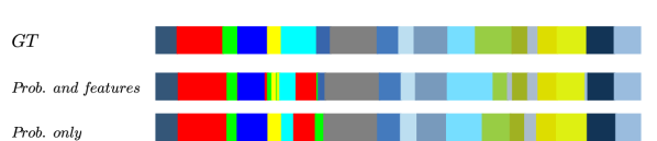
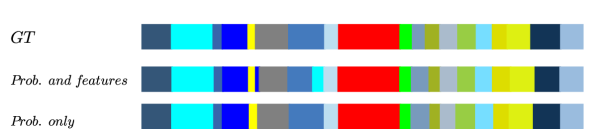
Figure 8: Qualitative results for two videos from the 50Salads dataset showing the effect of passing features to higher stages.

In the proposed multi-stage TCN, the input to higher stages are the frame-wise probabilities only. However, in the multi-stage architectures that are used for human pose estimation, additional features are usually concatenated to the output heat-maps of the previous stage. In this experiment, we therefore analyze the effect of combining additional features to the input probabilities of higher stages. To this end, we trained two multi-stage TCNs: one only with the predicted frame-wise probabilities as input to the next stage, and, for the second model, we concatenated the output of the last dilated convolutional layer in each stage to the input probabilities of the next stage. As shown in Table VI, concatenating the features to the input probabilities results in a huge drop of the F1 score and the segmental edit distance (around $20\%$). We argue that the reason behind this degradation in performance is that a lot of action classes share similar appearance and motion. By adding the features of such classes at each stage, the model is confused and produces small separated falsely detected action segments that correspond to an over-segmentation effect. Passing only the probabilities forces the model to focus on the context of neighboring labels, which are explicitly represented by the probabilities. This effect can also be seen in the qualitative results shown in Figure 8.

4.6 MS-TCN++ vs. MS-TCN

In this section, we compare the two multi-stage architectures: MS-TCN++ and MS-TCN. In contrast to MS-TCN, MS-TCN++ uses the dual dilated layer (DDL) in the first stage. Table VII shows the results of both architectures on the 50Salads dataset. As shown in the table, MS-TCN++ outperforms MS-TCN with a large margin of up to $6.4\%$. This emphasizes the importance of combining both local and global representations in the prediction generation stage by utilizing the DDL in MS-TCN++. To study the impact of using DDL in all stages, we also train an MS-TCN where we use the DDL in all stages. As shown in Table VII, MS-TCN++ outperforms MS-TCN with DDL in all stages. This indicates that decoupling the design of the refinement stages and the prediction generation stage is crucial. While utilizing the global context by the DDL is crucial for the prediction generation stage, the refinement stages focus more on the local context. By adding DDL to the refinement stages, the accuracy even drops due to overfitting. Note that using DDL in all stages outperforms MS-TCN with up to $2.8\%$. This further highlights the gains of the DDL. The impact of DDL is also visible in the qualitative results shown in Figure 9.

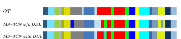
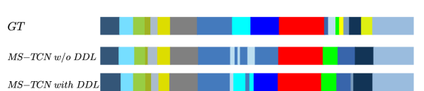
Figure 9: Qualitative results for two videos from the 50Salads dataset showing the impact of the dual dilated layer (DDL).

	F1@{10,25,50}			Edit	Acc
MS-TCN	76.3	74.0	64.5	67.9	80.7
MS-TCN with DDL	77.3	75.0	67.3	69.8	82.4
MS-TCN++	80.7	78.5	70.1	74.3	83.7

TABLE VII: MS-TCN++ vs. MS-TCN vs. MS-TCN with DDL on the 50Salads dataset.

4.7 Impact of the Number of Layers

For MS-TCN and the refinement stages in MS-TCN++, we fix the number of layers in each stage to $10$ layers. Whereas for the prediction generation stage in MS-TCN++, we set the number of layers to $11$. In this section, we study the impact of these parameters. Table VIII shows the impact of the number of layers ($L$) for the MS-TCN stages on the 50Salads dataset. Increasing $L$ form $8$ to $10$ significantly improves the performance. This is mainly due to the increase in the receptive field. Using more than $10$ layers ($L=11$, $L=12$) does not improve the frame-wise accuracy but slightly increases the F1 scores. We also tried to change the number of layers only in the refinement stages in MS-TCN. As shown in Table IX, this does not have a significant impact and using $10$ layers achieves the best performance. Also for the refinement stages in MS-TCN++, the number of layers $L_{r}$ does not have a significant impact on the performance. To be consistent with [14], we set $L_{r}=10$ which achieves a reasonable trade-off on performance with respect to all evaluation metrics as shown in Table IX. A similar behavior can be observed in Table X for the number of layers $L_{g}$ in the prediction generation stage with $L_{g}=11$ achieving the best performance. Generally speaking, the number of layers in each stage has more impact in MS-TCN compared to MS-TCN++. As the main difference between these two models is the dual dilation layer (DDL) that is used in MS-TCN++, this indicates that the DDL can better capture both local and global features to generate much better predictions.

	F1@{10,25,50}			Edit	Acc
$L$ = 6	53.2	48.3	39.0	46.2	63.7
$L$ = 8	66.4	63.7	52.8	60.1	73.9
$L$ = 10	76.3	74.0	64.5	67.9	80.7
$L$ = 11	76.7	74.2	65.5	69.7	80.4
$L$ = 12	77.8	75.2	66.9	69.6	80.5

TABLE VIII: Effect of the number of layers ($L$) in each stage of MS-TCN on the 50Salads dataset.

	F1@{10,25,50}			Edit	Acc
	$L_{r}$ = 6	74.3	71.5	62.8	66.0	78.6
	$L_{r}$ = 8	75.4	72.4	64.3	68.0	79.5
MS-TCN	$L_{r}$ = 10	76.3	74.0	64.5	67.9	80.7
	$L_{r}$ = 11	75.0	72.0	63.5	67.6	80.3
	$L_{r}$ = 12	74.1	71.2	62.3	65.7	79.1
	$L_{r}$ = 6	78.2	75.6	67.7	69.6	82.3
	$L_{r}$ = 8	80.9	78.2	70.2	73.4	82.9
MS-TCN++	$L_{r}$ = 10	80.7	78.5	70.1	74.3	83.7
	$L_{r}$ = 11	80.5	78.3	70.0	72.6	83.4
	$L_{r}$ = 12	79.4	76.9	69.2	71.3	83.5

TABLE IX: Effect of the number of layers ($L_{r}$) in each refinement stage on the 50Salads dataset.

	F1@{10,25,50}			Edit	Acc
$L_{g}$ = 6	74.3	71.6	63.5	67.8	78.5
$L_{g}$ = 8	77.4	75.3	67.8	70.3	80.8
$L_{g}$ = 10	79.8	77.9	71.0	72.5	83.1
$L_{g}$ = 11	80.7	78.5	70.1	74.3	83.7
$L_{g}$ = 12	78.9	76.6	67.6	70.8	83.2

TABLE X: Effect of the number of layers ($L_{g}$) in the prediction generation stage for MS-TCN++ on the 50Salads dataset.

4.8 Impact of the Large Receptive Field on Short Videos

To study the impact of the large receptive field on short videos, we evaluate MS-TCN and MS-TCN++ on three groups of videos based on their durations. For this evaluation, we use the GTEA dataset since it contains shorter videos compared to the other datasets. As shown in Table XI, both MS-TCN and MS-TCN++ perform well on both short and long videos. Nevertheless, the performance is slightly worse on longer videos due to the limited receptive field. The improvements of MS-TCN++ over MS-TCN are also noticeable for both short and long videos.

	Duration	F1@{10,25,50}			Edit	Acc
	$<1$ min	89.6	87.9	77.0	82.5	76.6
MS-TCN	$1-1.5$ min	85.9	84.3	71.9	80.7	76.4
	$\geq 1.5$ min	81.2	76.5	58.4	71.8	75.9
	$<1$ min	90.4	90.4	80.8	84.4	79.3
MS-TCN++	$1-1.5$ min	88.7	85.8	75.1	83.6	79.3
	$\geq 1.5$ min	80.8	78.8	63.3	76.1	77.2

TABLE XI: Evaluation of three groups of videos from the GTEA dataset based on their durations.

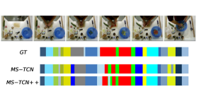
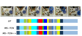
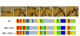
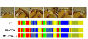
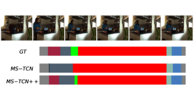
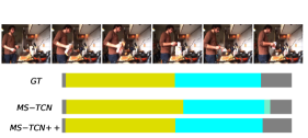
Figure 10: Qualitative results for the temporal action segmentation task on (a)(b) 50Salads, (c)(d) GTEA, and (e)(f) Breakfast dataset.

4.9 Effect of the Number of Refinement Stages

We set the number of refinement stages $N_{r}$ in MS-TCN++ to 3 stages, which results in a model with 4 stages in total. Table XII shows the impact of the refinement stages on the 50Salads dataset. Using only the prediction generation stage ($N_{r}=0$) results in a relative low performance but it is much better than a single stage TCN (Table II). Adding more refinement stages improves the performance incrementally. Nevertheless, adding more than 3 refinement stages does not provide additional improvements.

	$N_{r}$	F1@{10,25,50}			Edit	Acc
MS-TCN++	0	51.0	48.4	40.7	40.4	80.7
MS-TCN++	1	70.7	68.2	59.7	62.0	82.4
MS-TCN++	2	77.8	75.1	66.9	69.4	82.5
MS-TCN++	3	80.7	78.5	70.1	74.3	83.7
MS-TCN++	4	80.6	78.7	70.1	73.1	82.4

TABLE XII: Impact of the number of refinement stages on the 50Salads dataset.

4.10 Impact of Parameters Sharing

MS-TCN++ consists of a prediction generation stage and 3 refinement stages. Although adding more stages results in a better performance, it also increases the number of parameters. As the refinement stages share in principle the same task, it is hence intuitive that they can share parameters. Table XIII shows the impact of sharing parameters between the refinement stages. Sharing parameters significantly reduces the number of parameters with only a slight decrease in performance. For an MS-TCN++ with 3 refinement stages, sharing parameters reduces the total number of parameters to roughly $66\%$ of the total parameters in the original model. As shown in the table, MS-TCN++ with shared parameters outperforms MS-TCN with a margin of up to $3.8\%$ despite of having less parameters.

	F1@{10,25,50}			Edit	Acc	# param.(m)
MS-TCN	76.3	74.0	64.5	67.9	80.7	0.80
MS-TCN++	80.7	78.5	70.1	74.3	83.7	0.99
MS-TCN++(sh)	78.7	76.6	68.3	70.7	82.2	0.66

TABLE XIII: Impact of sharing parameters for the refinement stages on the 50Salads dataset.

4.11 Impact of Temporal Resolution

Previous temporal models operate on a low temporal resolution of 1-3 frames per second [11, 12, 13]. On the contrary, our approach is able to handle a higher resolution of 15 fps. In this experiment, we evaluate MS-TCN and MS-TCN++, with and without parameter sharing, for a low temporal resolution of 1 fps. As shown in Table XIV, both models are able to handle both low and high temporal resolutions. While reducing the temporal resolution for MS-TCN results in a better edit distance and segmental F1 score, using a higher resolution gives better frame-wise accuracy. Operating on a low temporal resolution makes MS-TCN less prone to the over-segmentation problem, which is reflected in the better edit and F1 scores. Due to the dual dilated layers, MS-TCN++ benefits more from a higher temporal resolution and the impact of reducing the temporal resolution for MS-TCN++ is noticeable for all evaluation metrics. Note that even when we share the parameters of the refinement stages in MS-TCN++, using a higher temporal resolution results in a better performance.

	F1@{10,25,50}			Edit	Acc
MS-TCN (1 fps)	77.8	74.9	64.0	70.7	78.6
MS-TCN (15 fps)	76.3	74.0	64.5	67.9	80.7
MS-TCN++ (1 fps)	80.4	78.7	68.6	73.3	81.1
MS-TCN++ (15 fps)	80.7	78.5	70.1	74.3	83.7
MS-TCN++(sh) (1 fps)	77.0	73.8	64.0	69.1	80.8
MS-TCN++(sh) (15 fps)	78.7	76.6	68.3	70.7	82.2

TABLE XIV: Impact of temporal resolution on the 50Salads dataset.

4.12 Impact of Fine-tuning the Features

In our experiments, we use the I3D features without fine-tuning. Table XV shows the effect of fine-tuning on the GTEA dataset. Both of our multi-stage architectures, MS-TCN and MS-TCN++, significantly outperform the single stage architecture - with and without fine-tuning. This also holds when the parameters of the refinement stages in MS-TCN++ are shared. Fine-tuning improves the results, but the effect of fine-tuning for action segmentation is lower than for action recognition. This is expected since the temporal model is by far more important for segmentation than for recognition.

Note that without fine-tuning, sharing parameters achieves better results on GTEA. This is mainly due to the reduced number of parameters, which prevents the model from over-fitting the training data, especially for small datasets like GTEA.

		F1@{10,25,50}			Edit	Acc
w/o FT	SS-TCN	62.8	60.0	48.1	55.0	73.3
	MS-TCN	85.8	83.4	69.8	79.0	76.3
	MS-TCN++	87.0	85.2	73.5	82.0	78.7
	MS-TCN++(sh)	87.8	86.2	74.4	82.6	78.9
with FT	SS-TCN	69.5	64.9	55.8	61.1	75.3
	MS-TCN	87.5	85.4	74.6	81.4	79.2
	MS-TCN++	88.8	85.7	76.0	83.5	80.1
	MS-TCN++(sh)	88.2	86.2	75.9	83.0	79.7

TABLE XV: Effect of fine-tuning on the GTEA dataset.

50Salads	F1@{10,25,50}			Edit	Acc
Spatial CNN[9]	32.3	27.1	18.9	24.8	54.9
IDT+LM[26]	44.4	38.9	27.8	45.8	48.7
Bi-LSTM[27]	62.6	58.3	47.0	55.6	55.7
Dilated TCN[11]	52.2	47.6	37.4	43.1	59.3
ST-CNN[9]	55.9	49.6	37.1	45.9	59.4
TUnet[48]	59.3	55.6	44.8	50.6	60.6
ED-TCN[11]	68.0	63.9	52.6	52.6	64.7
TResNet[49]	69.2	65.0	54.4	60.5	66.0
TRN[12]	70.2	65.4	56.3	63.7	66.9
TDRN+UNet[12]	69.6	65.0	53.6	62.2	66.1
TDRN[12]	72.9	68.5	57.2	66.0	68.1
LCDC+ED-TCN[31]	73.8	-	-	66.9	72.1
MS-TCN [14]	76.3	74.0	64.5	67.9	80.7
MS-TCN++(sh)	78.7	76.6	68.3	70.7	82.2
MS-TCN++	80.7	78.5	70.1	74.3	83.7
GTEA	F1@{10,25,50}			Edit	Acc
Spatial CNN[9]	41.8	36.0	25.1	-	54.1
Bi-LSTM[27]	66.5	59.0	43.6	-	55.5
Dilated TCN[11]	58.8	52.2	42.2	-	58.3
ST-CNN[9]	58.7	54.4	41.9	-	60.6
TUnet[48]	67.1	63.7	51.9	60.3	59.9
ED-TCN[11]	72.2	69.3	56.0	-	64.0
LCDC+ED-TCN[31]	75.4	-	-	72.8	65.3
TResNet[49]	74.1	69.9	57.6	64.4	65.8
TRN[12]	77.4	71.3	59.1	72.2	67.8
TDRN+UNet[12]	78.1	73.8	62.2	73.7	69.3
TDRN[12]	79.2	74.4	62.7	74.1	70.1
MS-TCN [14]	87.5	85.4	74.6	81.4	79.2
MS-TCN++(sh)	88.2	86.2	75.9	83.0	79.7
MS-TCN++	88.8	85.7	76.0	83.5	80.1
Breakfast	F1@{10,25,50}			Edit	Acc
ED-TCN [11]*	-	-	-	-	43.3
HTK [22]	-	-	-	-	50.7
TCFPN [13]	-	-	-	-	52.0
HTK(64) [8]	-	-	-	-	56.3
GRU [10]*	-	-	-	-	60.6
GRU+length prior [23]	-	-	-	-	61.3
MS-TCN (IDT) [14]	58.2	52.9	40.8	61.4	65.1
MS-TCN (I3D) [14]	52.6	48.1	37.9	61.7	66.3
MS-TCN++(I3D) (sh)	63.3	57.7	44.5	64.9	67.3
MS-TCN++ (I3D)	64.1	58.6	45.9	65.6	67.6

TABLE XVI: Comparison with the state-of-the-art on 50Salads, GTEA, and the Breakfast dataset. (* obtained from [13]).

4.13 Comparison with the State-of-the-Art

In this section, we compare the proposed models to the state-of-the-art methods on three datasets: 50Salads, Georgia Tech Egocentric Activities (GTEA), and the Breakfast datasets. The results are presented in Table XVI. As shown in the table, our models outperform the state-of-the-art methods on the three datasets and with respect to three evaluation metrics: F1 score, segmental edit distance, and frame-wise accuracy (Acc) with a large margin (up to $11.6\%$ for the frame-wise accuracy on the 50Salads dataset). Qualitative results on the three datasets are shown in Figure 10. Note that all the reported results are obtained using the I3D features. To analyze the effect of using a different type of features, we evaluated MS-TCN on the Breakfast dataset using the improved dense trajectories (IDT) features, which are the commonly used features for the Breakfast dataset. As shown in Table XVI, the impact of the features is very small. While the frame-wise accuracy and edit distance are slightly better using the I3D features, the model achieves a better F1 score when using the IDT features compared to I3D. This is mainly because I3D features encode both motion and appearance, whereas the IDT features encode only motion. For datasets like Breakfast, using appearance information does not help the performance since the appearance does not give a strong evidence about the action that is carried out. This can be seen in the qualitative results shown in Figure 10. The video frames share a very similar appearance. Additional appearance features therefore do not help in recognizing the activity. As shown in Table XVI, sharing the parameters of the refinement stages achieves similar performance to MS-TCN++, but it requires about $66\%$ less parameters as reported in Table XIII.

As our approaches do not use any recurrent layers, they are very fast both during training and testing. Training MS-TCN++ for $50$ epochs takes only $10$ minutes on the 50Salads dataset compared to $35$ minutes for training a single cell of a Bi-LSTM with a 64-dimensional hidden state on a single GTX 1080 Ti GPU. This is due to the sequential prediction of the LSTM, where the activations at any time step depend on the activations from the previous steps. For the MS-TCN and MS-TCN++, activations at all time steps are computed in parallel.

5 Conclusion

We presented two multi-stage architectures for the temporal action segmentation task. While the first stage generates an initial prediction, this prediction is iteratively refined by the higher stages. Instead of the commonly used temporal pooling, we used dilated convolutions to increase the temporal receptive field. The experimental evaluation demonstrated the capability of our architecture in capturing temporal dependencies between action classes and reducing over-segmentation errors. We further introduced a smoothing loss that gives an additional improvement of the predictions quality. We also introduced a dual dilated layer that captures both local and global features, which results in better performance. Moreover, we showed that sharing the parameters in the refinement stages results in a more efficient model with a slight degradation in performance. Our models outperform the state-of-the-art methods on three challenging datasets recorded from different views with a large margin. Since our model is fully convolutional, it is very efficient and fast both during training and testing.

Shijie Li received his Bachelor degree in Automation Engineering from University of Electronic Science and Technology of China in 2016 and his Master degree in computer science from the Nankai University in 2019. Since 2019, he is a PhD student at the University of Bonn. His research interests include action recognition and scene understanding.

Yazan Abu Farha received his Bachelor degree in computer systems engineering from Birzeit University in 2013 and his Master degree in computer science from the University of Bonn in 2017. Since 2018, he is a PhD student at the University of Bonn. His research interests include action recognition and anticipation.

Yun Liu is a PhD candidate at College of Computer Science, Nankai University. He received his bachelor degree from Nankai University in 2016. His research interests include computer vision and machine learning.

Ming-Ming Cheng received his PhD degree from Tsinghua University in 2012. Then he did 2 years research fellow, with Prof. Philip Torr in Oxford. He is now a professor at Nankai University, leading the Media Computing Lab. His research interests includes computer graphics, computer vision, and image processing. He received research awards including ACM China Rising Star Award, IBM Global SUR Award, and CCF-Intel Young Faculty Researcher Program. He is on the editorial boards of IEEE TIP.

Juergen Gall obtained his B.Sc. and his Masters degree in mathematics from the University of Wales Swansea (2004) and from the University of Mannheim (2005). In 2009, he obtained a Ph.D. in computer science from the Saarland University and the Max Planck Institut für Informatik. He was a postdoctoral researcher at the Computer Vision Laboratory, ETH Zurich, from 2009 until 2012 and senior research scientist at the Max Planck Institute for Intelligent Systems in Tübingen from 2012 until 2013. Since 2013, he is professor at the University of Bonn and head of the Computer Vision Group.

References

- [1] K. Simonyan and A. Zisserman, “Two-stream convolutional networks for action recognition in videos,” in Advances in Neural Information Processing Systems (NIPS), 2014, pp. 568–576.
- [2] C. Feichtenhofer, A. Pinz, and R. Wildes, “Spatiotemporal residual networks for video action recognition,” in Advances in Neural Information Processing Systems (NIPS), 2016, pp. 3468–3476.
- [3] J. Carreira and A. Zisserman, “Quo vadis, action recognition? A new model and the kinetics dataset,” in IEEE Conference on Computer Vision and Pattern Recognition (CVPR), 2017, pp. 4724–4733.
- [4] C. Feichtenhofer, H. Fan, J. Malik, and K. He, “Slowfast networks for video recognition,” in IEEE International Conference on Computer Vision (ICCV), 2019.
- [5] M. Rohrbach, S. Amin, M. Andriluka, and B. Schiele, “A database for fine grained activity detection of cooking activities,” in IEEE Conference on Computer Vision and Pattern Recognition (CVPR), 2012, pp. 1194–1201.
- [6] S. Karaman, L. Seidenari, and A. Del Bimbo, “Fast saliency based pooling of fisher encoded dense trajectories,” in European Conference on Computer Vision (ECCV), THUMOS Workshop, 2014.
- [7] D. Oneata, J. Verbeek, and C. Schmid, “The lear submission at THUMOS 2014,” 2014.
- [8] H. Kuehne, J. Gall, and T. Serre, “An end-to-end generative framework for video segmentation and recognition,” in IEEE Winter Conference on Applications of Computer Vision (WACV), 2016.
- [9] C. Lea, A. Reiter, R. Vidal, and G. D. Hager, “Segmental spatiotemporal CNNs for fine-grained action segmentation,” in European Conference on Computer Vision (ECCV). Springer, 2016, pp. 36–52.
- [10] A. Richard, H. Kuehne, and J. Gall, “Weakly supervised action learning with RNN based fine-to-coarse modeling,” in IEEE Conference on Computer Vision and Pattern Recognition (CVPR), 2017.
- [11] C. Lea, M. D. Flynn, R. Vidal, A. Reiter, and G. D. Hager, “Temporal convolutional networks for action segmentation and detection,” in IEEE Conference on Computer Vision and Pattern Recognition (CVPR), 2017.
- [12] P. Lei and S. Todorovic, “Temporal deformable residual networks for action segmentation in videos,” in IEEE Conference on Computer Vision and Pattern Recognition (CVPR), 2018, pp. 6742–6751.
- [13] L. Ding and C. Xu, “Weakly-supervised action segmentation with iterative soft boundary assignment,” in IEEE Conference on Computer Vision and Pattern Recognition (CVPR), 2018, pp. 6508–6516.
- [14] Y. Abu Farha and J. Gall, “MS-TCN: Multi-stage temporal convolutional network for action segmentation,” in IEEE Conference on Computer Vision and Pattern Recognition (CVPR), 2019.
- [15] S. Stein and S. J. McKenna, “Combining embedded accelerometers with computer vision for recognizing food preparation activities,” in ACM International Joint Conference on Pervasive and Ubiquitous Computing, 2013, pp. 729–738.
- [16] A. Fathi, X. Ren, and J. M. Rehg, “Learning to recognize objects in egocentric activities,” in IEEE Conference on Computer Vision and Pattern Recognition (CVPR), 2011, pp. 3281–3288.
- [17] H. Kuehne, A. Arslan, and T. Serre, “The language of actions: Recovering the syntax and semantics of goal-directed human activities,” in IEEE Conference on Computer Vision and Pattern Recognition (CVPR), 2014, pp. 780–787.
- [18] A. Fathi and J. M. Rehg, “Modeling actions through state changes,” in IEEE Conference on Computer Vision and Pattern Recognition (CVPR), 2013, pp. 2579–2586.
- [19] A. Fathi, A. Farhadi, and J. M. Rehg, “Understanding egocentric activities,” in IEEE International Conference on Computer Vision (ICCV), 2011, pp. 407–414.
- [20] S. Bhattacharya, M. M. Kalayeh, R. Sukthankar, and M. Shah, “Recognition of complex events: Exploiting temporal dynamics between underlying concepts,” in IEEE Conference on Computer Vision and Pattern Recognition (CVPR), 2014, pp. 2243–2250.
- [21] Y. Cheng, Q. Fan, S. Pankanti, and A. Choudhary, “Temporal sequence modeling for video event detection,” in IEEE Conference on Computer Vision and Pattern Recognition (CVPR), 2014, pp. 2227–2234.
- [22] H. Kuehne, A. Richard, and J. Gall, “Weakly supervised learning of actions from transcripts,” Computer Vision and Image Understanding, vol. 163, pp. 78–89, 2017.
- [23] H. Kuehne, A. Richard, and J. Gall, “A Hybrid RNN-HMM Approach for Weakly Supervised Temporal Action Segmentation,” IEEE Transactions on Pattern Analysis and Machine Intelligence, vol. 42, no. 04, pp. 765–779, 2020.
- [24] K. Tang, L. Fei-Fei, and D. Koller, “Learning latent temporal structure for complex event detection,” in IEEE Conference on Computer Vision and Pattern Recognition (CVPR), 2012, pp. 1250–1257.
- [25] N. N. Vo and A. F. Bobick, “From stochastic grammar to bayes network: Probabilistic parsing of complex activity,” in IEEE Conference on Computer Vision and Pattern Recognition (CVPR), 2014, pp. 2641–2648.
- [26] A. Richard and J. Gall, “Temporal action detection using a statistical language model,” in IEEE Conference on Computer Vision and Pattern Recognition (CVPR), 2016, pp. 3131–3140.
- [27] B. Singh, T. K. Marks, M. Jones, O. Tuzel, and M. Shao, “A multi-stream bi-directional recurrent neural network for fine-grained action detection,” in IEEE Conference on Computer Vision and Pattern Recognition (CVPR), 2016, pp. 1961–1970.
- [28] S. Singh, C. Arora, and C. V. Jawahar, “First person action recognition using deep learned descriptors,” in IEEE Conference on Computer Vision and Pattern Recognition (CVPR), 2016, pp. 2620–2628.
- [29] A. Van Den Oord, S. Dieleman, H. Zen, K. Simonyan, O. Vinyals, A. Graves, N. Kalchbrenner, A. W. Senior, and K. Kavukcuoglu, “Wavenet: A generative model for raw audio.” in ISCA Speech Synthesis Workshop (SSW), 2016.
- [30] S.-H. Gao, M.-M. Cheng, K. Zhao, X.-Y. Zhang, M.-H. Yang, and P. Torr, “Res2net: A new multi-scale backbone architecture,” IEEE Transactions on Pattern Analysis and Machine Intelligence, 2020.
- [31] K.-N. C. Mac, D. Joshi, R. A. Yeh, J. Xiong, R. S. Feris, and M. N. Do, “Learning motion in feature space: Locally-consistent deformable convolution networks for fine-grained action detection,” in IEEE International Conference on Computer Vision (ICCV), 2019.
- [32] Z. Shou, D. Wang, and S.-F. Chang, “Temporal action localization in untrimmed videos via multi-stage CNNs,” in IEEE Conference on Computer Vision and Pattern Recognition (CVPR), 2016.
- [33] H. Xu, A. Das, and K. Saenko, “R-C3D: Region convolutional 3d network for temporal activity detection,” in IEEE International Conference on Computer Vision (ICCV), 2017.
- [34] Y. Zhao, Y. Xiong, L. Wang, Z. Wu, X. Tang, and D. Lin, “Temporal action detection with structured segment networks,” in IEEE International Conference on Computer Vision (ICCV), 2017.
- [35] Y.-W. Chao, S. Vijayanarasimhan, B. Seybold, D. A. Ross, J. Deng, and R. Sukthankar, “Rethinking the faster R-CNN architecture for temporal action localization,” in IEEE Conference on Computer Vision and Pattern Recognition (CVPR), 2018.
- [36] R. Zeng, W. Huang, M. Tan, Y. Rong, P. Zhao, J. Huang, and C. Gan, “Graph convolutional networks for temporal action localization,” in IEEE International Conference on Computer Vision (ICCV), 2019.
- [37] J. Gao, Z. Yang, K. Chen, C. Sun, and R. Nevatia, “Turn tap: Temporal unit regression network for temporal action proposals,” in IEEE International Conference on Computer Vision (ICCV), 2017.
- [38] S. Buch, V. Escorcia, C. Shen, B. Ghanem, and J. Carlos Niebles, “SST: Single-stream temporal action proposals,” in IEEE Conference on Computer Vision and Pattern Recognition (CVPR), 2017.
- [39] J. Gao, Z. Yang, and R. Nevatia, “Cascaded boundary regression for temporal action detection,” in British Machine Vision Conference (BMVC), 2017.
- [40] T. Lin, X. Liu, X. Li, E. Ding, and S. Wen, “BMN: Boundary-matching network for temporal action proposal generation,” in IEEE International Conference on Computer Vision (ICCV), 2019, pp. 3889–3898.
- [41] S. Yeung, O. Russakovsky, G. Mori, and L. Fei-Fei, “End-to-end learning of action detection from frame glimpses in videos,” in IEEE Conference on Computer Vision and Pattern Recognition (CVPR), 2016.
- [42] S. Buch, V. Escorcia, B. Ghanem, L. Fei-Fei, and J. C. Niebles, “End-to-end, single-stream temporal action detection in untrimmed videos,” in British Machine Vision Conference (BMVC), 2017.
- [43] F. Long, T. Yao, Z. Qiu, X. Tian, J. Luo, and T. Mei, “Gaussian temporal awareness networks for action localization,” in IEEE Conference on Computer Vision and Pattern Recognition (CVPR), 2019.
- [44] S.-E. Wei, V. Ramakrishna, T. Kanade, and Y. Sheikh, “Convolutional pose machines,” in IEEE Conference on Computer Vision and Pattern Recognition (CVPR), 2016, pp. 4724–4732.
- [45] A. Newell, K. Yang, and J. Deng, “Stacked hourglass networks for human pose estimation,” in European Conference on Computer Vision (ECCV). Springer, 2016, pp. 483–499.
- [46] M. Dantone, J. Gall, C. Leistner, and L. Van Gool, “Body Parts Dependent Joint Regressors for Human Pose Estimation in Still Images,” IEEE Transactions on Pattern Analysis and Machine Intelligence, vol. 36, no. 11, pp. 2131–2143, 2014.
- [47] T.-Y. Lin, P. Dollár, R. Girshick, K. He, B. Hariharan, and S. Belongie, “Feature pyramid networks for object detection,” in IEEE Conference on Computer Vision and Pattern Recognition (CVPR), 2017.
- [48] O. Ronneberger, P. Fischer, and T. Brox, “U-net: Convolutional networks for biomedical image segmentation,” in International Conference on Medical Image Computing and Computer-Assisted Intervention. Springer, 2015, pp. 234–241.
- [49] K. He, X. Zhang, S. Ren, and J. Sun, “Deep residual learning for image recognition,” in IEEE Conference on Computer Vision and Pattern Recognition (CVPR), 2016, pp. 770–778.