FCOS: A Simple and Strong Anchor-free
Object Detector

Abstract

In computer vision, object detection is one of most important tasks, which underpins a few instance-level recognition tasks and many downstream applications. Recently one-stage methods have gained much attention over two-stage approaches due to their simpler design and competitive performance. Here we propose a fully convolutional one-stage object detector (FCOS) to solve object detection in a per-pixel prediction fashion, analogue to other dense prediction problems such as semantic segmentation. Almost all state-of-the-art object detectors such as RetinaNet, SSD, YOLOv3, and Faster R-CNN rely on pre-defined anchor boxes. In contrast, our proposed detector FCOS is anchor box free, as well as proposal free. By eliminating the pre-defined set of anchor boxes, FCOS completely avoids the complicated computation related to anchor boxes such as calculating the intersection over union (IoU) scores during training. More importantly, we also avoid all hyper-parameters related to anchor boxes, which are often sensitive to the final detection performance. With the only post-processing non-maximum suppression (NMS), we demonstrate a much simpler and flexible detection framework achieving improved detection accuracy. We hope that the proposed FCOS framework can serve as a simple and strong alternative for many other instance-level tasks. Code is available at: $\tt git.io/AdelaiDet$

1 Introduction

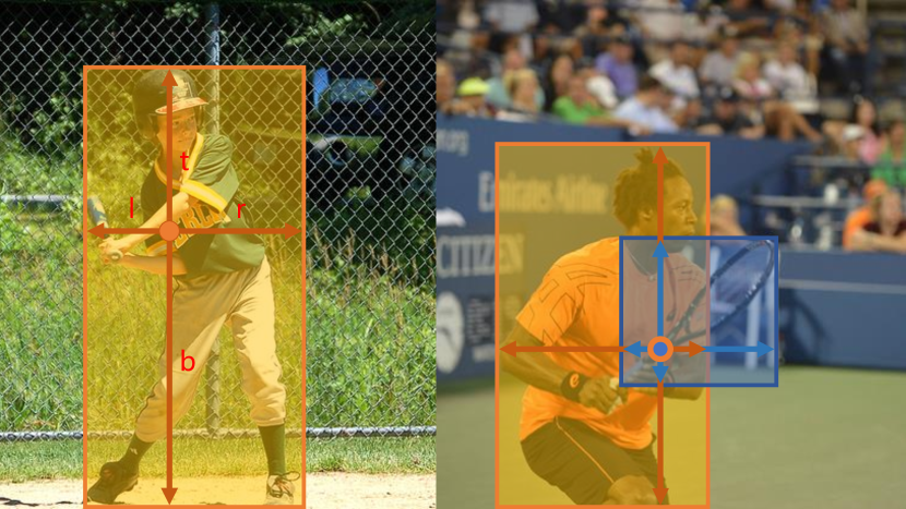
Figure 1: Overall concept of FCOS. As shown in the left image, FCOS works by predicting a 4D vector $(l,t,r,b)$ encoding the location of a bounding box at each foreground pixel (supervised by ground-truth bounding box information during training). The right plot shows that when a location residing in multiple bounding boxes, it can be ambiguous in terms of which bounding box this location should regress.

Object detection requires an algorithm to predict a bounding box location and a category label for each instance of interest in an image. Prior to deep learning, the sliding-window approach was the main method [1, 2, 3], which exhaustively classifies every possible location, thus requiring feature extraction and classification evaluation to be very fast. With deep learning, detection has been largely shifted to the use of fully convolutional networks (FCNs) since the invention of Faster R-CNN [4]. All current mainstream detectors such as Faster R-CNN [4], SSD [5] and YOLOv2, v3 [6] rely on a set of pre-defined anchor boxes and it has long been believed that the use of anchor boxes is the key to modern detectors’ success. Despite their great success, it is important to note that anchor-based detectors suffer some drawbacks:

• As shown in Faster R-CNN and RetinaNet [7], detection performance is sensitive to the sizes, aspect ratios and number of anchor boxes. For example, in RetinaNet, varying these hyper-parameters affects the performance up to $4\%$ in AP on the COCO benchmark [8]. As a result, these hyper-parameters need to be carefully tuned in anchor-based detectors.

• Even with careful design, because the scales and aspect ratios of anchor boxes are kept fixed, detectors encounter difficulties to deal with object candidates with large shape variations, particularly for small objects. The pre-defined anchor boxes also hamper the generalization ability of detectors, as they need to be re-designed on new detection tasks with different object sizes or aspect ratios.

• In order to achieve a high recall rate, an anchor-based detector is required to densely place anchor boxes on the input image (e.g., more than 180K anchor boxes in feature pyramid networks (FPN) [9] for an image with its shorter side being 800). Most of these anchor boxes are labeled as negative samples during training. The excessive number of negative samples aggravates the imbalance between positive and negative samples in training.

• Anchor boxes also involve complicated computation such as calculating the intersection-over-union (IoU) scores with ground-truth bounding boxes.

Recently, per-pixel prediction FCNs [10] have achieved tremendous success in dense prediction tasks such as semantic segmentation [10, 11, 12], depth estimation [13, 14], keypoint detection [15] and counting. As one of high-level vision tasks, object detection might be the only one deviating from the neat fully convolutional per-pixel prediction framework mainly due to the use of anchor boxes.

It is natural to ask a question: Can we solve object detection in the neat per-pixel prediction fashion, analogue to FCN for semantic segmentation, for example? Thus those fundamental vision tasks can be unified in (almost) one single framework. We show in this work that the answer is affirmative. Moreover, we demonstrate that, the much simpler FCN-based detector can surprisingly achieve even better performance than its anchor-based counterparts.

In the literature, some works attempted to leverage the per-pixel prediction FCNs for object detection such as DenseBox [16]. Specifically, these FCN-based frameworks directly predict a 4D vector plus a class category at each spatial location on a level of feature maps. As shown in Fig. 1 (left), the 4D vector depicts the relative offsets from the four sides of a bounding box to the location. These frameworks are similar to the FCNs for semantic segmentation, except that each location is required to regress a 4D continuous vector.

However, to handle the bounding boxes with different sizes, DenseBox [16] crops and resizes training images to a fixed scale. Thus DenseBox has to perform detection on image pyramids, which is against FCN’s philosophy of computing all convolutions once.

Besides, more significantly, these methods are mainly used in special domain objection detection such as scene text detection [17, 18] or face detection [19, 16], since it is believed that these methods do not work well when applied to generic object detection with highly overlapped bounding boxes. As shown in Fig. 1 (right), the highly overlapped bounding boxes result in an intractable ambiguity: it is not clear w.r.t. which bounding box to regress for the pixels in the overlapped regions.

In the sequel, we take a closer look at the issue and show that with FPN this ambiguity can be largely eliminated. As a result, our method can already obtain similar or even better detection accuracy with those traditional anchor based detectors. Furthermore, we observe that our method may produce a number of low-quality predicted bounding boxes at the locations that are far from the center of an target object. It is easy to see that the locations near the center of its target bounding box can make more reliable predictions. As a result, we introduce a novel “center-ness” score to depict the deviation of a location to the center, as defined in Eq. (3), which is used to down-weigh low-quality detected bounding boxes and thus helps to suppress these low-quality detections in NMS. The center-ness score is predicted by a branch (only one layer) in parallel with the bounding box regression branch, as shown in Fig. 2. The simple yet effective center-ness branch remarkably improves the detection performance with a negligible increase in computational time.

This new detection framework enjoys the following advantages.

• Detection is now unified with many other FCN-solvable tasks such as semantic segmentation, making it easier to re-use ideas from those tasks. An example is shown in [20], where a structured knowledge distillation method was developed for dense prediction tasks. Thanks to the standard FCN framework of FCOS, the developed technique can be immediately applied to FCOS based object detection.

• Detection becomes proposal free and anchor free, which significantly reduces the number of design parameters. The design parameters typically need heuristic tuning and many tricks are involved in order to achieve good performance. Therefore, our new detection framework makes the detector, particularly its training, considerably simpler.

• By eliminating the anchor boxes, our new detector completely avoids the complicated computation related to anchor boxes such as the IOU computation and matching between the anchor boxes and ground-truth boxes during training, resulting in faster training and testing than its anchor-based counterpart.

• Without bells and whistles, we achieve state-of-the-art results among one-stage detectors. Given its improved accuracy of the much simpler anchor-free detector, we encourage the community to rethink the necessity of anchor boxes in object detection, which are currently considered as the de facto standard for designing detection methods.

• With considerably reduced design complexity, our proposed detector outperforms previous strong baseline detectors such as Faster R-CNN [4], RetinaNet [7], YOLOv3 [6] and SSD [5]. More importantly, due to its simple design, FCOS can be easily extended to solve other instance-level recognition tasks with minimal modification, as already evidenced by instance segmentation [21, 22, 23, 24], keypoint detection [25], text spotting [26], and tracking [27, 28]. We expect to see more instance recognition methods built upon FCOS.

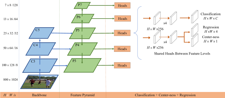
Figure 2: The network architecture of FCOS, where C3, C4, and C5 denote the feature maps of the backbone network and P3 to P7 are the feature levels used for the final prediction. $H\times W$ is the height and width of feature maps. ‘/$s$’ ($s=8,16,...,128$) is the down-sampling ratio of the feature maps at the level to the input image. As an example, all the numbers are computed with an $800\times 1024$ input.

1.1 Related Work

Here we review some work that is closest to ours.

Anchor-based Detectors.

Anchor-based detectors inherit the ideas from traditional sliding-window and proposal based detectors such as Fast R-CNN [29]. In anchor-based detectors, the anchor boxes can be viewed as pre-defined sliding windows or proposals, which are classified as positive or negative patches, with an extra offsets regression to refine the prediction of bounding box locations. Therefore, the anchor boxes in these detectors may be viewed as training samples. Unlike previous detectors like Fast RCNN, which compute image features for each sliding window/proposal repeatedly, anchor boxes make use of the feature maps of CNNs and avoid repeated feature computation, speeding up detection process dramatically. The design of anchor boxes are popularized by Faster R-CNN in its RPNs [4], SSD [5] and YOLOv2 [30], and has become the convention in a modern detector.

However, as described above, anchor boxes result in excessively many hyper-parameters, which typically need to be carefully tuned in order to achieve good performance. Besides the above hyper-parameters describing anchor shapes, the anchor-based detectors also need other hyper-parameters to label each anchor box as a positive, ignored or negative sample. In previous works, they often employ intersection over union (IOU) between anchor boxes and ground-truth boxes to determine the label of an anchor box (e.g., a positive anchor if its IOU is in $[0.5,1]$). These hyper-parameters have shown a great impact on the final accuracy, and require heuristic tuning. Meanwhile, these hyper-parameters are specific to detection tasks, making detection tasks deviate from a neat fully convolutional network architectures used in other dense prediction tasks such as semantic segmentation.

Anchor-free Detectors.

The most popular anchor-free detector might be YOLOv1 [31]. Instead of using anchor boxes, YOLOv1 predicts bounding boxes at points near the center of objects. Only the points near the center are used since they are considered to be able to produce higher-quality detection. However, since only points near the center are used to predict bounding boxes, YOLOv1 suffers from low recall as mentioned in YOLOv2 [30]. As a result, YOLOv2 [30] employs anchor boxes as well. Compared to YOLOv1, FCOS can take advantages of all points in a ground truth bounding box to predict the bounding boxes and the low-quality detected bounding boxes can be suppressed by the proposed “center-ness” branch. As a result, FCOS is able to provide comparable recall with anchor-based detectors as shown in our experiments.

CornerNet [32] is a recently proposed one-stage anchor-free detector, which detects a pair of corners of a bounding box and groups them to form the final detected bounding box. CornerNet requires much more complicated post-processing to group the pairs of corners belonging to the same instance. An extra distance metric is learned for the purpose of grouping.

Another family of anchor-free detectors such as [19] are based on DenseBox [16]. The family of detectors have been considered unsuitable for generic object detection due to difficulty in handling overlapping bounding boxes and the recall being relatively low. In this work, we show that both problems can be largely alleviated with multi-level prediction (i.e., FPNs). Moreover, we also show together with our proposed center-ness branch, the much simpler detector can achieve much better detection performance than its anchor-based counterparts. Recently, FSAF [33] was proposed to employ an anchor-free detection branch as a complement to an anchor-based detection branch since they consider that a totally anchor-free detector cannot achieve good performance. They also make use of a feature selection module to improve the performance of the anchor-free branch, making the anchor-free detector have a comparable performance to its anchor-based counterpart. However, in this work, we surprisingly show that the totally anchor-free detector can actually obtain better performance than its anchor-based counterpart, without the need for the feature selection module in FSAF. Even more surprisingly, it can outperform the combination of anchor-free and anchor-based detectors in FSAF. As a result, the long-standing anchor-boxes can be completely eliminated, making detection significantly simpler.

There are also some concurrent anchor-free detectors. For example, CenterNet [34] predicts the center, width and height of objects with hourglass networks, demonstrating promising performance. Compared to CenterNet, FCOS enjoys faster training, and has a better accuracy/speed trade-off, as shown in Table IX. RepPoints [35] represents the boxes by a set of points and uses converting functions to get the target boxes. In contrast, FCOS is a concise and very straightforward method for box detection.

After the submission of this work, some new anchor-free detectors appeared. For instance, CPN [36] replaces the region proposal networks (RPNs) in two-stage detectors with bottom-up anchor-free networks, achieving improved results. HoughNet [37] employs a voting mechanism to improve the performance of anchor-free bottom-up detection. These detectors require a grouping or voting post-processing, thus being considerably more complicated and slower than FCOS. There are also many follow-up works built upon FCOS [38, 39, 40, 41]. These works enhance the detection features, loss functions or the assigning strategy of FCOS, further boosting the anchor-free detector’s performance.

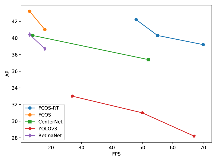
Figure 3: Speed/accuracy trade-off between FCOS and several recent methods: CenterNet [34], YOLOv3 [6] and RetinaNet [7]. Speed is measured on a NVIDIA 1080Ti GPU. For fair comparison, we only measure the network latency for all detectors. RetinaNet results are from ${{\tt Detectron2}}$. FCOS achieves competitive performance compared with recent methods including anchor-based ones.

2 Our Approach

In this section, we first reformulate object detection in a per-pixel prediction fashion. Next, we show that how we make use of multi-level prediction to improve the recall and resolve the ambiguity resulted from overlapped bounding boxes. Finally, we present our proposed “center-ness” branch, which helps suppress the low-quality detected bounding boxes and improves the overall performance by a large margin.

2.1 Fully Convolutional One-Stage Object Detector

Let $F_{i}\in{\mathbb{R}}^{H\times W\times C}$ be the feature maps at layer $i$ of a backbone CNN and $s$ be the total stride until the layer. The ground-truth bounding boxes for an input image are defined as $\{B_{i}\}$, where $B_{i}=(x^{(i)}_{0},y^{(i)}_{0},x^{(i)}_{1}y^{(i)}_{1},c^{(i)})\in{\mathbb{R}}^{4}\times\{1,2\ ...\ C\}$. Here $(x^{(i)}_{0},y^{(i)}_{0})$ and $(x^{(i)}_{1}y^{(i)}_{1})$ denote the coordinates of the left-top and right-bottom corners of the bounding box. $c^{(i)}$ is the class that the object in the bounding box belongs to. $C$ is the number of classes, which is $80$ for the MS-COCO dataset.

For each location $(x,y)$ on the feature map $F_{i}$, we can map it back onto the input image as $(\lfloor\frac{s}{2}\rfloor+xs,\left\lfloor\frac{s}{2}\right\rfloor+ys)$, which is near the center of the receptive field of the location $(x,y)$. Different from anchor-based detectors, which consider the location on the input image as the center of (multiple) anchor boxes and regress the target bounding box with these anchor boxes as references, we directly regress the target bounding box at the location. In other words, our detector directly views locations as training samples instead of anchor boxes in anchor-based detectors, which is the same as FCNs for semantic segmentation [10].

Specifically, location $(x,y)$ is considered as a positive sample if it falls into the center area of any ground-truth box, by following [42]. The center area of a box centered at $(c_{x},c_{y})$ is defined as the sub-box $(c_{x}-rs,c_{y}-rs,c_{x}+rs,c_{y}+rs)$, where $s$ is the total stride until the current feature maps and $r$ is a hyper-parameter being $1.5$ on COCO. The sub-box is clipped so that it is not beyond the original box. Note that this is different from our original conference version [43], where we consider the locations positive as long as they are in a ground-truth box. The class label $c^{*}$ of the location is the class label of the ground-truth box. Otherwise it is a negative sample and $c^{*}=0$ (background class). Besides the label for classification, we also have a 4D real vector $\boldsymbol{t}^{*}=(l^{*},t^{*},r^{*},b^{*})$ being the regression targets for the location. Here $l^{*}$, $t^{*}$, $r^{*}$ and $b^{*}$ are the distances from the location to the four sides of the bounding box, as shown in Fig. 1 (left). If a location falls into the center area of multiple bounding boxes, it is considered as an ambiguous sample. We simply choose the bounding box with minimal area as its regression target. In the next section, we will show that with multi-level prediction, the number of ambiguous samples can be reduced significantly and thus they hardly affect the detection performance. Formally, if location $(x,y)$ is associated to a bounding box $B_{i}$, the training regression targets for the location can be formulated as,

$$l^{*}=(x-x^{(i)}_{0})/s,~{}~{}t^{*}=(y-y^{(i)}_{0})/s,$$ (1)

$$r^{*}=(x^{(i)}_{1}-x)/s,~{}~{}b^{*}=(y^{(i)}_{1}-y)/s,$$

where $s$ is the total stride until the feature maps $F_{i}$, which is used to scale down regression targets and prevents the gradients from exploding during training. Together with these designs, FCOS can detect objects in an anchor-free way and everything is learned by the networks without the need for any pre-defined anchor-boxes. It is worth noting that this is not identical to an anchor-based detector with one anchor-box per location, the crucial difference is the way we define positive and negative samples. The single-anchor detector still uses pre-defined anchor-boxes as a prior and uses IoUs between the anchor-boxes and ground-truth boxes to determine the labels for these anchor-boxes. In FCOS, we remove the need for the prior and the locations are labeled by their inclusion in ground-truth boxes. In experiments, we will show that using a single anchor can only achieve inferior performance.

Network Outputs.

Corresponding to the training targets, the final layer of our networks predicts an 80D vector $\boldsymbol{p}$ for classification and a 4D vector $\boldsymbol{t}=(l,t,r,b)$ encoding bounding-box coordinates. Following [7], instead of training a multi-class classifier, we train $C$ binary classifiers. Similar to [7], we add two branches, respectively with four convolutional layers (exclude the final prediction layers) after the feature maps produced by FPNs for classification and regression tasks, respectively. Moreover, since the regression targets are always positive, we employ ${\rm ReLU}(x)$ to map any real number to $(0,\infty)$ on the top of the regression branch. It is worth noting that FCOS has $9\times$ fewer network output variables than the popular anchor-based detectors [7, 4] with 9 anchor boxes per location, which is of great importance when FCOS is applied to keypoint detection [25] or instance segmentation [44].

Loss Function.

We define our training loss function as follows:

$$L(\{\boldsymbol{p}_{x,y}\},\{\boldsymbol{t}_{x,y}\}) =\frac{1}{N_{{\rm pos}}}\sum_{x,y}{L_{{\rm cls}}(\boldsymbol{p}_{x,y},c^{*}_{x,y})}$$

$$+\frac{\lambda}{N_{{\rm pos}}}\sum_{{x,y}}{\mathbbm{1}_{\{c^{*}_{x,y}>0\}}L_{{\rm reg}}(\boldsymbol{t}_{x,y},\boldsymbol{t}^{*}_{x,y})},$$ (2)

where $L_{{\rm cls}}$ is focal loss as in [7] and $L_{{\rm reg}}$ is the GIoU loss [45]. As shown in experiments, the GIoU loss has better performance than the IoU loss in UnitBox [19], which is used in our preliminary version [43]. $N_{{\rm pos}}$ denotes the number of positive samples and $\lambda$ being $1$ in this paper is the balance weight for $L_{{\rm reg}}$. The summation is calculated over all locations on the feature maps $F_{i}$. $\mathbbm{1}_{\{c^{*}_{i}>0\}}$ is the indicator function, being $1$ if $c^{*}_{i}>0$ and $0$ otherwise.

Inference.

The inference of FCOS is straightforward. Given an input images, we forward it through the network and obtain the classification scores $\boldsymbol{p}_{x,y}$ and the regression prediction $\boldsymbol{t}_{x,y}$ for each location on the feature maps $F_{i}$. Following [7], we choose the location with $p_{x,y}>0.05$ as positive samples and invert Eq. (1) to obtain the predicted bounding boxes.

2.2 Multi-level Prediction with FPN for FCOS

Here we show that how two possible issues of the proposed FCOS can be resolved with multi-level prediction with FPN [9].

First, the large stride (e.g., 16$\times$) of the final feature maps in a CNN can result in a relatively low best possible recall (BPR). For anchor based detectors, low recall rates due to the large stride can be compensated to some extent by lowering the IOU score requirements for positive anchor boxes. For FCOS, at the first glance one may think that the BPR can be much lower than anchor-based detectors because it is impossible to recall an object which no location on the final feature maps encodes due to a large stride. Here, we empirically show that even with a large stride, FCOS is still able to produce a good BPR, and it can even better than the BPR of the anchor-based detector RetinaNet [7] in the official implementation Detectron [46] (refer to Table I). Therefore, the BPR is actually not a problem of FCOS. Moreover, with multi-level FPN prediction [9], the BPR can be improved further to match the best BPR the anchor-based RetinaNet can achieve.

Second, as shown in Fig. 1 (right), overlaps in ground-truth boxes can cause intractable ambiguity, i.e., which bounding box should a location in the overlap regress? This ambiguity results in degraded performance. In this work, we show that the ambiguity can be greatly resolved with multi-level prediction (and center sampling), and FCOS can obtain on par, sometimes even better, performance compared with anchor-based ones.

Specifically, following FPN [9], we detect different size objects on different feature map levels. we make use of five levels of feature maps defined as $\{P_{3},P_{4},P_{5},P_{6},P_{7}\}$. As shown in Fig. 2, $P_{3}$, $P_{4}$ and $P_{5}$ are produced by the backbone CNNs’ feature maps $C_{3}$, $C_{4}$ and $C_{5}$ with the top-down connections as in [9]. $P_{6}$ and $P_{7}$ are produced by applying one $3\times 3$ convolutional layer with the stride being 2 on $P_{5}$ and $P_{6}$, respectively. Note that this is different from the original RetinaNet, which obtain $P_{6}$ and $P_{7}$ from the backbone feature maps $C_{5}$. We find both schemes achieve similar performance but the one we use has fewer parameters. Moreover, the feature levels $P_{3}$, $P_{4}$, $P_{5}$, $P_{6}$ and $P_{7}$ have strides 8, 16, 32, 64 and 128, respectively.

Anchor-based detectors assign different scale anchor boxes to different feature levels. Since anchor boxes and ground-boxes are associated by their IoU scores, this enables different FPN feature levels to handle different scale objects. However, this couples the sizes of anchor boxes and the target object sizes of each FPN level, which is problematic. The anchor box sizes should be data-specific, which might be changed from one dataset to another. The target object sizes of each FPN level should depend on the receptive field of the FPN level, which depends on the network architecture. FCOS removes the coupling as we only need focus on the target object sizes of each FPN level and need not design the anchor box sizes. Unlike anchor-based detectors, in FCOS, we directly limit the range of bounding box regression for each level. More specifically, we first compute the regression targets $l^{*}$, $t^{*}$, $r^{*}$ and $b^{*}$ for each location on all feature levels. Next, if a location at feature level $i$ satisfies $\max(l^{*}$, $t^{*},r^{*},b^{*})\leq m_{i-1}$ or $\max(l^{*},t^{*},r^{*},b^{*})\geq m_{i}$, it is set as a negative sample and thus not required to regress a bounding box anymore. Here $m_{i}$ is the maximum distance that feature level $i$ needs to regress. In this work, $m_{2}$, $m_{3}$, $m_{4}$, $m_{5}$, $m_{6}$ and $m_{7}$ are set as $0$, $64$, $128$, $256$, $512$ and $\infty$, respectively. We argue that bounding the maximum distance is a better way to determine the range of target objects for each feature level because this makes sure that the complete objects are always in the receptive field of each feature level. Moreover, since objects of different sizes are assigned to different feature levels and overlapping mostly happens between objects with considerably different sizes, the aforementioned ambiguity can be largely alleviated. If a location, even with multi-level prediction used, is still assigned to more than one ground-truth boxes, we simply choose the ground-truth box with minimal area as its target. As shown in our experiments, with the multi-level prediction, both anchor-free and anchor-based detectors can achieve the same level performance.

Finally, following [9, 7], we share the heads between different feature levels, not only making the detector parameter-efficient but also improving the detection performance. However, we observe that different feature levels are required to regress different size range (e.g., the size range is $[0,64]$ for $P_{3}$ and $[64,128]$ for $P_{4}$), and therefore it may not be the optimal design to make use of identical heads for different feature levels. In our preliminary version [43], this issue is addressed by multiplying a learnable scalar to the convolutional layer’s outputs. In this version, since the regression targets are scaled down by the stride of FPN feature levels, as shown in Eq. (1), the scalars become less important. However, we still keep them for compatibility.

2.3 Center-ness for FCOS

After using multi-level prediction, FCOS can already achieve better performance than its anchor-based counterpart RetinaNet. Furthermore, we observed that there are a lot of low-quality detections produced by the locations far away from the center of an object.

We propose a simple yet effective strategy to suppress these low-quality detections. Specifically, we add a single-layer branch, in parallel with the regression branch (as shown in Fig. 2) to predict the “center-ness” of a location. The center-ness depicts the normalized distance from the location to the center of the object that the location is responsible for, as shown Fig. 4. Given the regression targets $l^{*}$, $t^{*}$, $r^{*}$ and $b^{*}$ for a location, the center-ness target is defined as,

$${\rm centerness}^{*}=\sqrt{\frac{\min(l^{*},r^{*})}{\max(l^{*},r^{*})}\times\frac{\min(t^{*},b^{*})}{\max(t^{*},b^{*})}}.$$ (3)

We employ $\rm sqrt$ here to slow down the decay of the center-ness. The center-ness ranges from $0$ to $1$ and is thus trained with binary cross entropy (BCE) loss. The loss is added to the loss function Eq. (2.1). When testing, the final score $\boldsymbol{s}_{x,y}$ (used for ranking the detections in NMS) is the square root of the product of the predicted center-ness $o_{x,y}$ and the corresponding classification score $\boldsymbol{p}_{x,y}$. Formally,

$$\boldsymbol{s}_{x,y}=\sqrt{\boldsymbol{p}_{x,y}\times o_{x,y}},$$ (4)

where $\rm sqrt$ is used to calibrate the order of magnitude of the final score and has no effect on average precision (AP).

Consequently, center-ness can down-weight the scores of bounding boxes far from the center of an object. As a result, with high probability, these low-quality bounding boxes might be filtered out by the final non-maximum suppression (NMS) process, improving the detection performance remarkably.

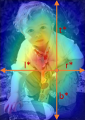
Figure 4: Center-ness. Red, blue, and other colors denote 1, 0 and the values between them, respectively. Center-ness is computed using Eq. (3) and decays from 1 to 0 as the location deviates from the center of the object. During testing, the center-ness predicted by the network is multiplied with the classification score for NMS, thus being able to down-weight the low-quality bounding boxes predicted by a location far from the center of an object.

3 Experiments

Our experiments are conducted on the large-scale detection benchmark COCO [8]. Following the common practice [7, 9, 4], we use the COCO ${{\tt train2017}}$ split (115K images) for training and ${{\tt val2017}}$ split (5K images) as validation for our ablation study. We report our main results on the ${{\tt test}}$-dev split (20K images) by uploading our detection results to the evaluation server.

Training Details.

Unless specified, we use the following implementation details. ResNet-50 [47] is used as our backbone networks and the same hyper-parameters with RetinaNet [7] are used. Specifically, our network is trained with stochastic gradient descent (SGD) for 90k iterations with the initial learning rate being 0.01 and a mini-batch of 16 images. The learning rate is reduced by a factor of 10 at iteration 60k and 80k, respectively. Weight decay and momentum are set as 0.0001 and 0.9, respectively. We initialize our backbone networks with the weights pre-trained on ImageNet [48]. For the newly added layers, we initialize them as in [7]. Unless specified, the input images are resized to have their shorter side being 800 and their longer side less or equal to 1333.

Inference Details.

We firstly forward the input image through the network and obtain the predicted bounding boxes with the predicted class scores. The next post-processing of FCOS exactly follows that of RetinaNet [7]. The post-processing hyper-parameters are also the same except that we use NMS threshold $0.6$ instead of $0.5$ in RetinaNet. Experiments will be conducted to show the effect of the NMS threshold. Moreover, we use the same sizes of input images as in training.

3.1 Analysis of FCOS

3.1.1 Best Possible Recall (BPR) of FCOS

Method	w/ FPN	Low-quality matches	BPR (%)
RetinaNet	✓	Not used	88.16
RetinaNet	✓	$\geq 0.4$	91.94
RetinaNet	✓	All	99.32
FCOS		-	96.34
FCOS	✓	-	98.95

TABLE I: The best possible recall (BPR) of anchor-based RetinaNet under a variety of matching rules and the BPR of FCOS on the COCO ${{\tt val2017}}$ split. FCOS has very similar BPR to the best anchor-based one and has much higher recall than the official implementation in ${{\tt Detectron}}$ [46], where only low-quality matches with IOU $\geq 0.4$ are considered.

w/ ctr. sampling	w/ FPN	$1$	$2$	$\geq 3$
		$76.60\%$	$20.05\%$	$3.35\%$
	✓	$92.58\%$	$6.97\%$	$0.45\%$
✓		$96.52\%$	$3.34\%$	$0.14\%$
✓	✓	$97.34\%$	$2.59\%$	$0.07\%$

TABLE II: The ratios of the ambiguous samples to all the positive samples in FCOS. $1,2$ and $\geq 3$ denote the number of ground-truth boxes a location should be associated to. If the number is greater than $1$, the location is defined as an “ambiguous sample” in this work. As shown in the table, with center sampling and FPN, the ratio of ambiguous samples is low (i.e., $<3\%$).

Method	AP	AP50	AP75	APS	APM	APL	AR1	AR10	AR100	ARS	ARM	ARL
RetinaNet (#A=9)	35.9	55.8	38.4	20.6	39.8	46.6	31.0	49.8	53.0	33.8	57.4	67.9
RetinaNet (#A=1) w/ imprv.	35.2	55.6	37.0	19.9	39.2	45.2	30.4	49.9	53.5	33.6	57.7	68.2
RetinaNet (#A=9) w/ imprv.	37.6	56.6	40.6	21.5	42.1	48.0	32.1	52.2	56.4	35.5	60.2	72.7
FCOS w/o ctr.-ness	38.0	57.2	40.9	21.5	42.4	49.1	32.1	52.4	56.2	36.6	60.6	71.9
FCOS w/ ctr.-ness	38.9	57.5	42.2	23.1	42.7	50.2	32.4	53.8	57.5	38.5	62.1	72.9

TABLE III: FCOS vs. RetinaNet on ${{\tt val2017}}$ split with ResNet-50-FPN as the backbone. All experiments use the same training settings. The proposed anchor-free FCOS achieves even better performance than anchor-based RetinaNet. #A: the number of anchors per location. RetinaNet (#A=9): the original RetinaNet from ${{\tt Detectron2}}$ [49]. RetinaNet w/ imprv. RetinaNet with the universal improvements in FCOS including Group Normalization (GN) [50], GIoU loss [42] and scalars in regression, using $P_{5}$ instead of $C_{5}$ and NMS threshold $0.6$ instead of $0.5$. We have tried our best to make all the details consistent. As shown the table, even without the center-ness branch, the much simpler FCOS already outperforms ”RetinaNet (#A=9) w/ imprv” by $0.4\%$ in AP. With the center-ness branch, the performance is further improved to $38.9\%$ in AP.

We first address the concern that is FCOS might not provide a good best possible recall (BPR) (i.e., upper bound of the recall rate). In the section, we show that the concern is not necessary by comparing BPR of FCOS and that of its anchor-based counterpart RetinaNet on the COCO ${{\tt val2017}}$ split. The following analyses are based on the FCOS implementation in ${{\tt AdelaiDet}}$. Formally, BPR is defined as the ratio of the number of ground-truth boxes that a detector can recall at the most to the number of all ground-truth boxes. A ground-truth box is considered recalled if the box is assigned to at least one training sample (i.e., a location in FCOS or an anchor box in anchor-based detectors), and a training sampling can be associated to at most one ground-truth box. As shown in Table I, both with FPN, FCOS and RetinaNet obtain similar BPR ($98.95$ vs $99.32$). Due to the fact that the best recall of current detectors are much lower than $90\%$, the small BPR gap (less than $0.5\%$) between FCOS and the anchor-based RetinaNet will not actually affect the performance of a detector. It is also confirmed in Table III, where FCOS achieves better or similar AR than RetinaNet under the same training and testing settings. Even more surprisingly, only with feature level $P_{4}$ with stride being 16 (i.e., no FPN), FCOS can obtain a decent BPR of $96.34\%$. The BPR is much higher than the BPR of $91.94\%$ of the RetinaNet in the official implementation ${{\tt Detectron}}$ [46], where only the low-quality matches with IOU $\geq 0.4$ are used. Therefore, the concern about low BPR may not be necessary.

3.1.2 Ambiguous Samples in FCOS

Another concern about the FCN-based detector is that it may have a large number of ambiguous samples due to the overlap in ground-truth boxes, as shown in Fig. 1 (right). In Table II, we show the ratios of the ambiguous samples to all positive samples on ${{\tt val2017}}$ split. If a location should be associated to multiple ground-truth boxes without using the rule of choosing the box with minimum area, the location is defined as an “ambiguous sample”. As shown in the table, there are indeed a large amount of ambiguous samples ($23.40\%$) if FPN is not used (i.e., only $P_{4}$ used). However, with FPN, the ratio can be significantly reduced to only $7.42\%$ since most of overlapped objects are assigned to different feature levels. Furthermore, if the center sampling is used, the ambiguous samples can be significantly reduced. As shown in Table II, even without FPN, th ratio is only $3.48\%$. By further applying FPN, the ratio is reduced to $2.66\%$. Note that it does not imply that there are $2.66\%$ locations where FCOS makes mistakes. As mentioned before, these locations are associated with the smallest one among the ground-truth boxes associated to the same location. Therefore, these locations only take the risk of missing some larger objects. In other words, it may harm the recall of FCOS. However, as shown in Table I, the recall gap between FCOS and RetinaNet is negligible, which suggests that the ratio of the missing objects is extremely low.

3.1.3 The Effect of Center-ness

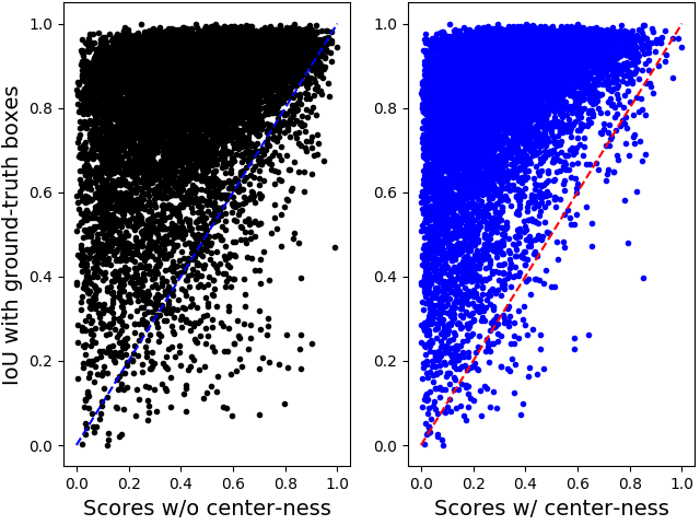
Figure 5: Quantitative results of applying the center-ness scores to classification scores. A point in the figure denotes a bounding box. The dashed line is the line $y=x$. As shown in the right figure, after applying the center-ness scores, the boxes with low IoU scores but high confidence scores (i.e., under the line $y=x$) are reduced substantially.

	AP	AP50	AP75	APS	APM	APL
w/o ctr.-ness	38.0	57.2	40.9	21.5	42.4	49.1
w/ ctr.-ness†	37.5	56.5	40.2	21.6	41.5	48.5
w/ ctr.-ness (L1)	38.9	57.6	42.0	23.0	42.3	51.0
w/ ctr.-ness	38.9	57.5	42.2	23.1	42.7	50.2

TABLE IV: Ablation study for the proposed center-ness branch on the ${{\tt val2017}}$ split. ctr.-ness^†: using the center-ness computed from the predicted regression vector when testing (i.e., replacing the ground-truth values with the predicted ones in Eq. (3)). “ctr.-ness” is that using center-ness predicted from the proposed center-ness branch. The center-ness branch improves the detection performance. On the contrary, using “ctr.-ness^†” even degrades the performance, which suggests that the separate center-ness branch is necessary. w/ ctr.-ness (L1): using L1 instead of BCE as the loss to optimize the center-ness.

As mentioned before, we propose “center-ness” to suppress the low-quality detected bounding boxes produced by the locations far from the center of an object. As shown in Table IV, the center-ness branch can boost AP from $38.0\%$ to $38.9\%$. Compared to our conference version [43], the gap is relatively smaller since we make use of the center sampling by default and it already eliminates a large number of false positives. However, the improvement is still impressive as the center-ness branch only adds negligible computational time. Moreover, we will show later that the center-ness can bring a large improvement in crowded scenarios. One may note that center-ness can also be computed with the predicted regression vector without introducing the extra center-ness branch. However, as shown in Table IV, the center-ness computed from the regression vector cannot improve the performance and thus the separate center-ness is necessary.

We visualize the effect of applying the center-ness in Fig. 4. As shown in the figure, after applying the center-ness scores to the classification scores, the boxes with low IoU scores but high confidence scores are largely eliminated (i.e., the points under the line $y=x$ in the Fig. 4), which are potential false positives.

	AP	AP50	AP75	APS	APM	APL
Baseline	38.9	57.5	42.2	23.1	42.7	50.2
w/o GN	37.9	56.4	40.9	22.1	41.8	48.8
w/ IoU	38.6	57.2	41.9	22.4	42.1	49.8
w/ C5	38.5	57.4	41.7	22.8	42.1	49.3

TABLE V: Ablation study for design choices in FCOS. w/o GN: without using Group Normalization (GN) for the convolutional layers in heads. w/ IoU: using IoU loss in [19] instead of GIoU. w/ $C_{5}$: using $C_{5}$ instead of $P_{5}$.

$r$	AP	AP50	AP75	APS	APM	APL
$1.0$	38.5	57.2	41.5	22.6	42.3	49.7
$1.5$	38.9	57.5	42.2	23.1	42.7	50.2
$2.0$	38.8	57.7	41.7	22.7	42.6	49.9

TABLE VI: Ablation study for the radius $r$ of positive sample regions (defined in Section 2.1).

Strategy	AP	AP50	AP75	APS	APM	APL
FPN	37.7	56.6	40.6	22.2	40.9	49.7
$\sqrt{(h^{*}\times w^{*})}/2$	37.6	56.5	40.6	22.4	41.6	47.3
${\rm max}(h^{*},w^{*})/2$	38.1	57.0	41.3	22.5	41.8	48.7
${\rm max}(l^{*},t^{*},r^{*},b^{*})$	38.9	57.5	42.2	23.1	42.7	50.2

TABLE VII: Ablation study for different strategies of assigning objects to FPN levels. FPN: the strategy of assigning object proposals (i.e., ROIs) to FPN levels in the original FPN, described in the text. $h^{*}$ and $w^{*}$ are the height and width of a ground-truth box, respectively. $l^{*}$, $t^{*}$, $r^{*}$ and $b^{*}$ are the distances from a location to the four boundaries of a ground-truth box. “$\rm max$$(l^{*},t^{*},r^{*},b^{*})$” (used by FCOS) has the best performance.

3.1.4 Other Design Choices

Other design choices are also investigated. As shown Table V, removing group normalization (GN) [50] in both the classification and regression heads drops the performance by $1\%$ AP. By replacing GIoU [45] with the origin IoU loss in [19], the performance drops by $0.3\%$ AP. Using $C_{5}$ instead of $P_{5}$ also degrades the performance. Moreover, using $P_{5}$ can reduce the number of the network parameters. We also conduct experiments for the radius $r$ of positive sample regions. As shown in Table VI, $r=1.5$ has the best performance on COCO ${{\tt val}}$ split. We also attempted to change the sampling area from square sub-boxes to the rectangle sub-boxes with the same aspect ratio as the ground-truth boxes, which results in similar performance. It suggests that the shape of the sampling area may be not sensitive to the final performance.

We also conduct experiments with different strategies of assigning objects to FPN levels. First, we experiment with the assigning strategy when FPN [9] assigns the object proposals (i.e., ROIs) to FPN levels. It assigns the objects according to the formulation $k=\lfloor k_{0}+{\rm log}_{2}({\sqrt{wh}/224})\rfloor$, where $k\in\{3,4,5,6,7\}$ is the target FPN level, $w$ and $h$ are the ground-truth box’s width and height, respectively, and $k_{0}$ is the target level which an object with scale $224$ should be mapped into. We use $k_{0}=5$. As shown in Table VII, this strategy results in degraded performance ($37.7\%$ AP). We conjecture that it may be because the strategy cannot make sure the complete object be within the receptive field of the target FPN level.

Similarly, $\sqrt{(h^{*}\times w^{*})}/2$ and ${\rm max}(h^{*},w^{*})/2$ also deteriorate the performance. Eventually, ${\rm max}(l^{*},t^{*},r^{*},b^{*})$ achieves the best performance as the strategy makes sure that the complete target objects are always in the effective receptive field of the FPN level. Moreover, this implies that the range hyper-parameters of each FPN level (i.e., $m_{i}$) is mainly related to the network architecture (which determines the receptive fields). This is a desirable feature since it eliminates the hyper-parameter tuning when FCOS is applied to different datasets.

3.2 FCOS vs. Anchor-based Counterparts

Here, we compare FCOS with its anchor-based counterpart RetinaNet on the challenging benchmark COCO, demonstrating that the much simpler anchor-free FCOS is superior.

In order to make a fair comparison, we add the universal improvements in FCOS to RetinaNet. The improved RetinaNet is denoted as “RetinaNet w/ imprv.” in Table III. As shown the table, even without the center-ness branch, FCOS achieves $0.4\%$ better AP than “RetinaNet (#A=9) w/ imprv.” ($38.0\%$ vs $37.6\%$ in AP). The performance of FCOS can be further boosted to $38.9\%$ with the help of the proposed center-ness branch. Moreover, it is worth noting that FCOS achieves much better performance than the RetinaNet with a single anchor per location “RetinaNet (#A=1) w/ imprv.” ($38.0\%$ vs $35.2\%$), which suggests that FCOS is not equivalent to the single-anchor RetinaNet. The major difference is FCOS does not employ IoU scores between anchor boxes and ground-truth boxes to determine the training labels.

Given the superior performance and merits of the anchor-free detector (e.g., much simpler and fewer hyper-parameters), we encourage the community to rethink the necessity of anchor boxes in object detection.

3.3 Comparison with State-of-the-art Detectors on COCO

Method	Backbone	AP	AP50	AP75	APS	APM	APL
Two-stage methods:
Faster R-CNN+++ [47]	ResNet-101	34.9	55.7	37.4	15.6	38.7	50.9
Faster R-CNN w/ FPN [9]	ResNet-101-FPN	36.2	59.1	39.0	18.2	39.0	48.2
Faster R-CNN by G-RMI [51]	Inception-ResNet-v2 [52]	34.7	55.5	36.7	13.5	38.1	52.0
Faster R-CNN w/ TDM [53]	Inception-ResNet-v2-TDM	36.8	57.7	39.2	16.2	39.8	52.1
One-stage methods:
YOLOv2 [30]	DarkNet-19 [30]	21.6	44.0	19.2	5.0	22.4	35.5
SSD513 [5]	ResNet-101-SSD	31.2	50.4	33.3	10.2	34.5	49.8
YOLOv3 $608\times 608$ [6]	Darknet-53	33.0	57.9	34.4	18.3	35.4	41.9
DSSD513 [54]	ResNet-101-DSSD	33.2	53.3	35.2	13.0	35.4	51.1
RetinaNet [7]	ResNet-101-FPN	39.1	59.1	42.3	21.8	42.7	50.2
CornerNet [32]	Hourglass-104	40.5	56.5	43.1	19.4	42.7	53.9
FSAF [33]	ResNeXt-64x4d-101-FPN	42.9	63.8	46.3	26.6	46.2	52.7
CenterNet511 [55]	Hourglass-104	44.9	62.4	48.1	25.6	47.4	57.4
FCOS	ResNet-101-FPN	43.2	62.4	46.8	26.1	46.2	52.8
FCOS	ResNeXt-32x8d-101-FPN	44.1	63.7	47.9	27.4	46.8	53.7
FCOS	ResNeXt-64x4d-101-FPN	44.8	64.4	48.5	27.7	47.4	55.0
FCOS w/ deform.  conv.  v2 [56]	ResNeXt-32x8d-101-FPN	46.6	65.9	50.8	28.6	49.1	58.6
FCOS	ResNet-101-BiFPN [57]	45.0	63.6	48.7	27.0	47.9	55.9
FCOS	ResNeXt-32x8d-101-BiFPN	46.2	65.2	50.0	28.7	49.1	56.5
FCOS w/ deform.  conv.  v2	ResNeXt-32x8d-101-BiFPN	47.9	66.9	51.9	30.2	50.3	59.9
w/ test-time augmentation:
FCOS	ResNet-101-FPN	45.9	64.5	50.4	29.4	48.3	56.1
FCOS	ResNeXt-32x8d-101-FPN	47.0	66.0	51.6	30.7	49.4	57.1
FCOS	ResNeXt-64x4d-101-FPN	47.5	66.4	51.9	31.4	49.7	58.2
FCOS w/ deform.  conv.  v2	ResNeXt-32x8d-101-FPN	49.1	68.0	53.9	31.7	51.6	61.0
FCOS	ResNet-101-BiFPN	47.9	65.9	52.5	31.0	50.7	59.7
FCOS	ResNeXt-32x8d-101-BiFPN	49.0	67.4	53.6	32.0	51.7	60.5
FCOS w/ deform.  conv.  v2	ResNeXt-32x8d-101-BiFPN	50.4	68.9	55.0	33.2	53.0	62.7

TABLE VIII: FCOS vs. other state-of-the-art two-stage or one-stage detectors (single-model results). FCOS outperforms a few recent anchor-based and anchor-free detectors by a considerable margin.

We compare FCOS with other state-of-the-art object detectors on ${{\tt test}}$-${{\tt dev}}$ split of MS-COCO benchmark. For these experiments, following previous works [7, 5], we make use of multi-scale training. To be specific, during training, the shorter side of the input image is sampled from $[640,800]$ with a step of $32$. Moreover, we double the number of iterations to 180K (with the learning rate change points scaled proportionally). Other settings are exactly the same as the model with AP $38.9\%$ on ${{\tt val2017}}$ in Table III.

As shown in Table VIII, with ResNet-101-FPN, FCOS outperforms the original RetinaNet with the same backbone by $4.1\%$ AP ($43.2\%$ vs $39.1\%$). Compared to other one-stage detectors such as SSD [5] and DSSD [54], we also achieve much better performance. Moreover, FCOS also surpasses the classical two-stage anchor-based detector Faster R-CNN by a large margin ($43.2\%$ vs.  $36.2\%$). To our knowledge, it is the first time that an anchor-free detector, without any bells and whistles, outperforms anchor-based detectors by a large margin. Moreover, FCOS also outperforms the previous anchor-free detector CornerNet [32] and CenterNet [55] while being much simpler since they requires to group corners with embedding vectors, which needs special design for the detector. Thus, we argue that FCOS is more likely to serve as a strong and simple alternative to current mainstream anchor-based detectors. Quantitative results are shown in Fig. 6. It appears that FCOS works well with a variety of challenging cases.

We also introduce some complementary techniques to FCOS. First, deformable convolutions are used in stages $3$ and $4$ of the backbone, and also replace the last convolutional layers in the classification and regression towers (i.e., the $4\times$ convolutions shown in Fig. 2). As shown in Table VIII, by applying deformable convolutions [58, 56] to ResNeXt-32x8d-101-FPN based FCOS, the performance is improved from $44.1\%$ to $46.6\%$ AP, as shown in Table VIII. In addition, we also attempt to replace FPN in FCOS with BiFPN [57]. We make use of BiFPN in D3 model in [57]. To be specific, the single cell of BiFPN is repeated $6$ times and the number of its output channels is set to $160$. Note that unlike the original BiFPN, we do not employ depthwise separable convolutions in it. As a result, BiFPN generally improves all FCOS models by $\sim 2\%$ AP and pushes the performance of the best model to $47.9\%$.

We also report the result of using test-time data augmentation. Specifically, in inference, the input image is respectively resized to $[400,1200]$ pixels with step $100$. At each scale, the original image and its horizontal flip are evaluated. The results from these augmented images are merged by NMS. As shown in Table VIII, the test-time augmentation improves the best performance to $50.4\%$ AP.

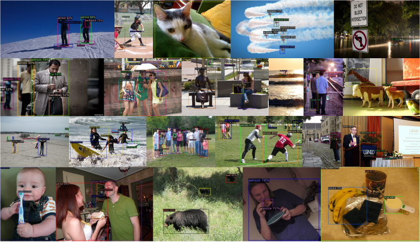
Figure 6: Qualitative results. As shown in the figure, FCOS works well with a wide range of objects including crowded, occluded, extremely small and very large objects.

3.4 Real-time FCOS

Method	FPS	AP	AP ${{\tt test}}$-${{\tt dev}}$
YOLOv3 (Darknet-53) [6]	26	$-$	33.0
CenterNet (DLA-34) [34]	52	37.4	37.3
FCOS-RT (R-50)	38	40.2	40.2
FCOS-RT (DLA-34-BiFPN)	43	42.1	42.2
FCOS-RT (DLA-34)	46	40.3	40.3
FCOS-RT w/ shtw. (DLA-34)	52	39.1	39.2

TABLE IX: Real-time FCOS (FCOS-RT) models. AP is on COCO ${{\tt val}}$ split. “shtw.”: sharing towers (i.e., $4\times$ conv. layers shown in Fig. 2) between the classification and regression branches. The inference time is measured with a single 1080Ti or Titan XP GPU (these two GPUs’ speeds are close). FPS of all FCOS models is measured on a 1080Ti GPU. We measure the FPS of YOLOv3 on 1080Ti using the code released by [6]. For FCOS and YOLOv3, we measure the end-to-end inference time here (i.e., from prepossessing to the final output boxes).

We also design a real-time version FCOS-RT. In the real-time settings, we reduce the shorter side of input images from $800$ to $512$ and the maximum longer size from $1333$ to $736$, which decreases the inference time per image by $\sim 50\%$. With the smaller input size, the higher feature levels $P_{6}$ and $P_{7}$ become less important. Thus, following BlendMask-RT [24], we remove $P_{6}$ and $P_{7}$, further reducing the inference time. Moreover, in order to boost the performance of the real-time version, we employ a more aggressive training strategy. Specifically, during training, multi-scale data augmentation is used and the shorter size of input image is sampled from $256$ to $608$ with interval $32$. Synchronized batch normalization (SyncBN) is used. We also increase the training iterations to $360K$ (i.e., $4\times$). The learning rate is decreased by a factor of $10$ at iteration $300K$ and $340K$.

The resulting real-time models are shown in Table IX. With ResNet-50, FCOS-RT can achieve $40.2\%$ AP at $38$ FPS on a single 1080Ti GPU card. We further replace ResNet-50 with the backbone DLA-34 [59], which results in a better speed/accuracy trade-off ($40.3\%$ AP at $46$ FPS). In order to compare with CenterNet[34], we share the towers (i.e., $4\times$ conv. layers shown in Fig. 2) between the classification and regression branches, which improves the speed from $46$ FPS to $52$ FPS but deteriorate the performance by $1.2\%$ AP. However, as shown in Table IX, the model still outperforms CenterNet [34] by $1.7\%$ AP at the same speed. For the real-time models, we also replace FPN with BiFPN as in Section 3.3, resulting $1.8\%$ AP improvement (from $40.3\%$ to $42.1\%$) at similar speed. A speed/accuracy comparison between FCOS and a few recent detection methods is shown in Fig. 3.

3.5 FCOS on CrowdHuman

Figure 7: Qualitative results on the CrowdHuman ${{\tt val}}$ set with the ResNet-50-FPN backbone.

	AP	MR-2	JI
RetinaNet w/ imprv.	81.60	57.36	72.88
FCOS w/o ctr.-ness	83.16	59.04	73.09
FCOS w/ ctr.-ness	85.0	51.34	74.97
$+$ MIP ($K=2$)	85.19	51.60	75.14
$+$ Set NMS [60]	87.28	51.21	77.34

TABLE X: FCOS for crowded object detection on the CrowdHuman dataset. Even on the highly crowded benchmark, FCOS still attains even better performance than anchor-based RetinaNet. Note that lower MR^-2 is better. “MIP w. set NMS”: Multiple Instance Prediction, which predicts multiple instances from a single location as proposed by [60]. Note that we are not pursuing the state-of-the-art performance on the benchmark. We only show that the anchor boxes are not necessary even on the highly-crowded benchmark.

We also conduct experiments on the highly crowded dataset CrowdHuman [61]. CrowdHuman consists of $15k$ images for training, $4,370$ for validation and $5,000$ images for testing. Following previous works on crowded benchmark [60, 61], we use AP, long-average Miss Rate on False Positive Per Image in $[10^{-2},100]$ (MR^-2) [62] and Jaccard Index (JI) as the evaluation metrics. Note that lower MR^-2 is better. Following [60], all experiments here are trained on the ${{\tt train}}$ split for $30$ epochs with batch size $16$ and then evaluated on the ${{\tt val}}$ split. Two some changes are made when FCOS is applied to the benchmark. First, the NMS threshold is set as $0.5$ instead of $0.6$. We find that it has large impact on MR^-2 and JI. Second, when a location is supposed to be associated to multiple ground-truth boxes, on COCO, we choose the object with minimal area as the target for the location. On CrowdHuman, we instead choose the target with minimal distance to the location. The distance between a location and an object is defined as the distance from the location to the center of the object. On COCO, both schemes result in similar performance. However, the latter has much better performance than the former on the highly crowded dataset. Other settings are the same as that of COCO.

First, we count the ambiguous sample ratios on CrowdHuman ${{\tt val}}$ set. With FPN-based FCOS, there are $84.47\%$ unambiguous positive samples (with one ground-truth box), $13.63\%$ with two ground-truth boxes, $1.69\%$ with three ground-truth boxes and the rest ($<0.3\%$) with more than three ground-truth boxes. Given the much higher ambiguous sample ratio than COCO, it is expected that FCOS will have inferior performance on the highly crowded dataset.

We compare FCOS without center-ness with the the improved RetinaNet (i.e., “RetinaNet w/ imprv.”). To our surprise, even without center-ness, FCOS can already achieve decent performance. As shown in Table X, FCOS compares favorably with its anchor-based counterpart RetinaNet on two out of three metrics (AP and JI), which suggests that anchor-based detectors have no large advantages even under the highly crowded scenario. The higher MR^-2 of FCOS denotes that FCOS might have a large number of false positives with high confidence. By using the center-ness, MR^-2 can be significantly reduced from $59.04\%$ to $51.34\%$. As a result, FCOS can achieve better results under all the three metrics.

Furthermore, as shown in [60], it is more reasonable to let one proposal make multiple predictions under the highly crowded scenario (i.e., multiple instance prediction (MIP)). After that, these predictions are merged by Set NMS [60], which skips the suppression for the boxes from the same location. A similar idea can be easily incorporated into FCOS. To be specific, if a location should be associated to multiple objects, instead of choosing a single target (i.e., the closest one to the location), the location’s targets are set as the $K$-closest objects. Accordingly, the network is required to make $K$ predictions per location. Moreover, we do not make use of the earth mover’s distance (EMD) loss for simplicity. Finally, the results are merged by Set NMS [60]. As shown in Table X, with MIP and Set NMS, improved performance is achieved under all the three metrics.

4 Conclusion

In this work, we have proposed an anchor-free and proposal-free one-stage detector FCOS. Our experiments demonstrate that FCOS compares favourably against the widely-used anchor-based one-stage detectors, including RetinaNet, YOLO and SSD, but with much less design complexity. FCOS completely avoids all computation and hyper-parameters related to anchor boxes and solves the object detection in a per-pixel prediction fashion, similar to other dense prediction tasks such as semantic segmentation. FCOS also achieves state-of-the-art performance among one-stage detectors. We also present some real-time models of our detector, which have state-of-the-art performance and inference speed. Given its effectiveness and efficiency, we hope that FCOS can serve as a strong and simple alternative of current mainstream anchor-based detectors.

Zhi Tian is a PhD student at School of Computer Science, The University of Adelaide, Australia. He received his B.E. degree in Computer Science and Technology from Sichuan University, China. He was awarded a Google PhD fellowship in 2019.

Chunhua Shen is a Professor at School of Computer Science, The University of Adelaide, Australia.

Hao Chen is a PhD student at School of Computer Science, The University of Adelaide, Australia. He received his BSc and master degrees from Zhejiang University, China.

Tong He is a postdoc researcher at The University of Adelaide. He did his PhD study at the same university. He received his master degree from Wuhan University, China.

References

- [1] P. Viola and M. Jones, “Robust real-time object detection,” Int. J. Comp. Vis., 2001.
- [2] C. Shen, P. Wang, S. Paisitkriangkrai, and A. van den Hengel, “Training effective node classifiers for cascade classification,” Int. J. Comp. Vis., vol. 103, no. 3, pp. 326–347, 2013.
- [3] P. Dollár, R. Appel, S. Belongie, and P. Perona, “Fast feature pyramids for object detection,” IEEE Trans. Pattern Anal. Mach. Intell., 2014.
- [4] S. Ren, K. He, R. Girshick, and J. Sun, “Faster R-CNN: Towards real-time object detection with region proposal networks,” in Proc. Adv. Neural Inf. Process. Syst., pp. 91–99, 2015.
- [5] W. Liu, D. Anguelov, D. Erhan, C. Szegedy, S. Reed, C.-Y. Fu, and A. C. Berg, “SSD: Single shot multibox detector,” in Proc. Eur. Conf. Comp. Vis., pp. 21–37, Springer, 2016.
- [6] J. Redmon and A. Farhadi, “Yolov3: An incremental improvement,” arXiv preprint arXiv:1804.02767, 2018.
- [7] T.-Y. Lin, P. Goyal, R. Girshick, K. He, and P. Dollár, “Focal loss for dense object detection,” in Proc. IEEE Conf. Comp. Vis. Patt. Recogn., pp. 2980–2988, 2017.
- [8] T.-Y. Lin, M. Maire, S. Belongie, J. Hays, P. Perona, D. Ramanan, P. Dollár, and L. Zitnick, “Microsoft COCO: Common objects in context,” in Proc. Eur. Conf. Comp. Vis., pp. 740–755, Springer, 2014.
- [9] T.-Y. Lin, P. Dollár, R. Girshick, K. He, B. Hariharan, and S. Belongie, “Feature pyramid networks for object detection,” in Proc. IEEE Conf. Comp. Vis. Patt. Recogn., pp. 2117–2125, 2017.
- [10] J. Long, E. Shelhamer, and T. Darrell, “Fully convolutional networks for semantic segmentation,” in Proc. IEEE Conf. Comp. Vis. Patt. Recogn., pp. 3431–3440, 2015.
- [11] Z. Tian, T. He, C. Shen, and Y. Yan, “Decoders matter for semantic segmentation: Data-dependent decoding enables flexible feature aggregation,” in Proc. IEEE Conf. Comp. Vis. Patt. Recogn., pp. 3126–3135, 2019.
- [12] T. He, C. Shen, Z. Tian, D. Gong, C. Sun, and Y. Yan, “Knowledge adaptation for efficient semantic segmentation,” in Proc. IEEE Conf. Comp. Vis. Patt. Recogn., June 2019.
- [13] F. Liu, C. Shen, G. Lin, and I. Reid, “Learning depth from single monocular images using deep convolutional neural fields,” IEEE Trans. Pattern Anal. Mach. Intell., 2016.
- [14] W. Yin, Y. Liu, C. Shen, and Y. Yan, “Enforcing geometric constraints of virtual normal for depth prediction,” in Proc. IEEE Int. Conf. Comp. Vis., 2019.
- [15] Y. Chen, C. Shen, X.-S. Wei, L. Liu, and J. Yang, “Adversarial PoseNet: A structure-aware convolutional network for human pose estimation,” in Proc. IEEE Int. Conf. Comp. Vis., 2017.
- [16] L. Huang, Y. Yang, Y. Deng, and Y. Yu, “Densebox: Unifying landmark localization with end to end object detection,” arXiv preprint arXiv:1509.04874, 2015.
- [17] X. Zhou, C. Yao, H. Wen, Y. Wang, S. Zhou, W. He, and J. Liang, “EAST: an efficient and accurate scene text detector,” in Proc. IEEE Conf. Comp. Vis. Patt. Recogn., pp. 5551–5560, 2017.
- [18] T. He, Z. Tian, W. Huang, C. Shen, Y. Qiao, and C. Sun, “An end-to-end textspotter with explicit alignment and attention,” in Proc. IEEE Conf. Comp. Vis. Patt. Recogn., pp. 5020–5029, 2018.
- [19] J. Yu, Y. Jiang, Z. Wang, Z. Cao, and T. Huang, “Unitbox: An advanced object detection network,” in Proc. ACM Int. Conf. Multimedia, pp. 516–520, ACM, 2016.
- [20] Y. Liu, C. Shun, J. Wang, and C. Shen, “Structured knowledge distillation for dense prediction,” IEEE Trans. Pattern Anal. Mach. Intell., 2020.
- [21] E. Xie, P. Sun, X. Song, W. Wang, X. Liu, D. Liang, C. Shen, and P. Luo, “PolarMask: Single shot instance segmentation with polar representation,” in Proc. IEEE Conf. Comp. Vis. Patt. Recogn., 2020. arxiv.org/abs/1909.13226.
- [22] R. Zhang, Z. Tian, C. Shen, M. You, and Y. Yan, “Mask encoding for single shot instance segmentation,” in Proc. IEEE Conf. Comp. Vis. Patt. Recogn., 2020.
- [23] Y. Lee and J. Park, “CenterMask: Real-time anchor-free instance segmentation,” in Proc. IEEE Conf. Comp. Vis. Patt. Recogn., 2020.
- [24] H. Chen, K. Sun, Z. Tian, C. Shen, Y. Huang, and Y. Yan, “BlendMask: Top-down meets bottom-up for instance segmentation,” in Proc. IEEE Conf. Comp. Vis. Patt. Recogn., 2020.
- [25] Z. Tian, H. Chen, and C. Shen, “DirectPose: Direct end-to-end multi-person pose estimation,” arXiv preprint arXiv:1911.07451, 2019.
- [26] Y. Liu, H. Chen, C. Shen, T. He, L. Jin, and L. Wang, “ABCNet: Real-time scene text spotting with adaptive Bezier-curve network,” in Proc. IEEE Conf. Comp. Vis. Patt. Recogn., 2020.
- [27] G. Wang, C. Luo, X. Sun, Z. Xiong, and W. Zeng, “Tracking by instance detection: A meta-learning approach,” in Proc. IEEE Conf. Comp. Vis. Patt. Recogn., 2020.
- [28] D. Guo, J. Wang, Y. Cui, Z. Wang, and S. Chen, “SiamCAR: Siamese fully convolutional classification and regression for visual tracking,” in Proc. IEEE Conf. Comp. Vis. Patt. Recogn., 2020.
- [29] R. Girshick, “Fast R-CNN,” in Proc. IEEE Conf. Comp. Vis. Patt. Recogn., pp. 1440–1448, 2015.
- [30] J. Redmon and A. Farhadi, “YOLO9000: better, faster, stronger,” in Proc. IEEE Conf. Comp. Vis. Patt. Recogn., pp. 7263–7271, 2017.
- [31] J. Redmon, S. Divvala, R. Girshick, and A. Farhadi, “You only look once: Unified, real-time object detection,” in Proc. IEEE Conf. Comp. Vis. Patt. Recogn., pp. 779–788, 2016.
- [32] H. Law and J. Deng, “Cornernet: Detecting objects as paired keypoints,” in Proc. Eur. Conf. Comp. Vis., pp. 734–750, 2018.
- [33] C. Zhu, Y. He, and M. Savvides, “Feature selective anchor-free module for single-shot object detection,” in Proc. IEEE Conf. Comp. Vis. Patt. Recogn., June 2019.
- [34] X. Zhou, D. Wang, and P. Krähenbühl, “Objects as points,” in arXiv preprint arXiv:1904.07850, 2019.
- [35] Z. Yang, S. Liu, H. Hu, L. Wang, and S. Lin, “Reppoints: Point set representation for object detection,” in Proc. IEEE Int. Conf. Comp. Vis., pp. 9657–9666, 2019.
- [36] K. Duan, L. Xie, H. Qi, S. Bai, Q. Huang, and Q. Tian, “Corner proposal network for anchor-free, two-stage object detection,” in Proc. Eur. Conf. Comp. Vis., 2020.
- [37] N. Samet, S. Hicsonmez, and E. Akbas, “HoughNet: Integrating near and long-range evidence for bottom-up object detection,” in Proc. Eur. Conf. Comp. Vis., 2020.
- [38] H. Qiu, Y. Ma, Z. Li, S. Liu, and J. Sun, “BorderDet: Border feature for dense object detection,” in Proc. Eur. Conf. Comp. Vis., 2020.
- [39] X. Li, W. Wang, L. Wu, S. Chen, X. Hu, J. Li, J. Tang, and J. Yang, “Generalized focal loss: Learning qualified and distributed bounding boxes for dense object detection,” in Proc. Adv. Neural Inf. Process. Syst., 2020.
- [40] S. Zhang, C. Chi, Y. Yao, Z. Lei, and S. Z. Li, “Bridging the gap between anchor-based and anchor-free detection via adaptive training sample selection,” in Proc. IEEE Conf. Comp. Vis. Patt. Recogn., pp. 9759–9768, 2020.
- [41] B. Zhu, J. Wang, Z. Jiang, F. Zong, S. Liu, Z. Li, and J. Sun, “Autoassign: Differentiable label assignment for dense object detection,” arXiv preprint arXiv:2007.03496, 2020.
- [42] https://github.com/yqyao/FCOS_PLUS, 2019.
- [43] Z. Tian, C. Shen, H. Chen, and T. He, “FCOS: Fully convolutional one-stage object detection,” in Proc. IEEE Int. Conf. Comp. Vis., 2019.
- [44] Z. Tian, C. Shen, and H. Chen, “Conditional convolutions for instance segmentation,” in Proc. Eur. Conf. Computer Vision (ECCV), 2020.
- [45] H. Rezatofighi, N. Tsoi, J. Gwak, A. Sadeghian, I. Reid, and S. Savarese, “Generalized intersection over union: A metric and a loss for bounding box regression,” in Proc. IEEE Conf. Comp. Vis. Patt. Recogn., pp. 658–666, 2019.
- [46] R. Girshick, I. Radosavovic, G. Gkioxari, P. Dollár, and K. He, “Detectron.” https://github.com/facebookresearch/detectron, 2018.
- [47] K. He, X. Zhang, S. Ren, and J. Sun, “Deep residual learning for image recognition,” in Proc. IEEE Conf. Comp. Vis. Patt. Recogn., pp. 770–778, 2016.
- [48] J. Deng, W. Dong, R. Socher, L.-J. Li, K. Li, and L. Fei-Fei, “ImageNet: A large-scale hierarchical image database,” in Proc. IEEE Conf. Comp. Vis. Patt. Recogn., pp. 248–255, IEEE, 2009.
- [49] Y. Wu, A. Kirillov, F. Massa, W.-Y. Lo, and R. Girshick, “Detectron2.” https://github.com/facebookresearch/detectron2, 2019.
- [50] Y. Wu and K. He, “Group normalization,” in Proc. Eur. Conf. Comp. Vis., pp. 3–19, 2018.
- [51] J. Huang, V. Rathod, C. Sun, M. Zhu, A. Korattikara, A. Fathi, I. Fischer, Z. Wojna, Y. Song, S. Guadarrama, and K. Murphy, “Speed/accuracy trade-offs for modern convolutional object detectors,” in Proc. IEEE Conf. Comp. Vis. Patt. Recogn., pp. 7310–7311, 2017.
- [52] C. Szegedy, S. Ioffe, V. Vanhoucke, and A. A. Alemi, “Inception-v4, inception-resnet and the impact of residual connections on learning,” in Proc. AAAI Conf. Artificial Intell., 2017.
- [53] A. Shrivastava, R. Sukthankar, J. Malik, and A. Gupta, “Beyond skip connections: Top-down modulation for object detection,” in Proc. IEEE Conf. Comp. Vis. Patt. Recogn., 2017.
- [54] C.-Y. Fu, W. Liu, A. Ranga, A. Tyagi, and A. Berg, “DSSD: Deconvolutional single shot detector,” arXiv preprint arXiv:1701.06659, 2017.
- [55] K. Duan, S. Bai, L. Xie, H. Qi, Q. Huang, and Q. Tian, “CenterNet: Keypoint triplets for object detection,” in Proc. IEEE Int. Conf. Comp. Vis., pp. 6569–6578, 2019.
- [56] X. Zhu, H. Hu, S. Lin, and J. Dai, “Deformable convnets v2: More deformable, better results,” in Proc. IEEE Conf. Comp. Vis. Patt. Recogn., pp. 9308–9316, 2019.
- [57] M. Tan, R. Pang, and Q. Le, “EfficientDet: Scalable and efficient object detection,” in Proc. IEEE Conf. Comp. Vis. Patt. Recogn., 2020.
- [58] J. Dai, H. Qi, Y. Xiong, Y. Li, G. Zhang, H. Hu, and Y. Wei, “Deformable convolutional networks,” in Proc. IEEE Int. Conf. Comp. Vis., pp. 764–773, 2017.
- [59] F. Yu, D. Wang, E. Shelhamer, and T. Darrell, “Deep layer aggregation,” in Proc. IEEE Conf. Comp. Vis. Patt. Recogn., pp. 2403–2412, 2018.
- [60] X. Chu, A. Zheng, X. Zhang, and J. Sun, “Detection in crowded scenes: One proposal, multiple predictions,” in Proc. IEEE Conf. Comp. Vis. Patt. Recogn., 2020.
- [61] S. Shao, Z. Zhao, B. Li, T. Xiao, G. Yu, X. Zhang, and J. Sun, “Crowdhuman: A benchmark for detecting human in a crowd,” arXiv preprint arXiv:1805.00123, 2018.
- [62] P. Dollar, C. Wojek, B. Schiele, and P. Perona, “Pedestrian detection: An evaluation of the state of the art,” IEEE Trans. Pattern Anal. Mach. Intell., vol. 34, no. 4, pp. 743–761, 2011.