Iterative Nadaraya-Watson Distribution Transfer for Colour Grading

Abstract

We propose a new method with Nadaraya-Watson that maps one N-dimensional distribution to another taking into account available information about correspondences. We extend the 2D/3D problem to higher dimensions by encoding overlapping neighborhoods of data points and solve the high dimensional problem in 1D space using an iterative projection approach. To show potentials of this mapping, we apply it to colour transfer between two images that exhibit overlapped scene. Experiments show quantitative and qualitative improvements over previous state of the art colour transfer methods.

I Introduction

Colour variations between photographs often happen due to illumination changes, using different cameras, different in-camera settings or due to tonal adjustments of the users. Colour transfer methods have been developed to transform a source colour image into a specified target colour image to match colour statistics or eliminate colour variations between different photographs. Applications of colour transfer in image processing problems are various, ranging from colour correction for image mosaicing and stitching [1], to colour enhancement and style manipulation for artistic design applications [2]. An example of application of colour transfer is illustrated in Figure 2: light fields have become a major research topic and among the different methods used to capture a light field are the lenslet cameras that extract sub-aperture images (SAI), each with a very wide depth of field and representing different viewpoints of the scene. However, as can be seen, the extracted views suffer from a number of artifacts such as colour discrepancies [3, 4].

When target and source images are from the same scene, correspondences can be found to guide the process for recolouring [5]. The SIFT flow algorithm [6] is well suited for matching densely sampled, pixel-wise SIFT features between the two images [7] and is used in our proposed pipeline (cf. Fig. 1). In this paper, we propose to use these correspondences between source and target images for performing colour transfer with a new algorithm (cf. Sec. II) noted INWDT (cf. Fig. 1). We compare our approach against state of the art techniques for colour transfer [8, 2, 9, 5, 10] (Sec. III) and show competitive results, both quantitatively and qualitatively.

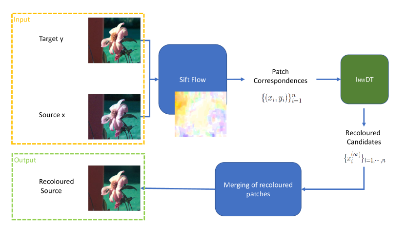
Figure 1: Proposed Pipeline: Following [7], correspondences between target and source are found using SIFT flow [6]. These correspondences are used in our proposed INWDT algorithm (cf. Alg. 1) to compute recoloured candidates that are then merged using the same process as [10] to compose the recoloured source image.

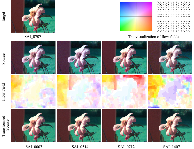
Figure 2: Results on SAI light fields images. Our method NW_cp successfully corrects colour inconsistencies in the selected outer views images using the centre view image (SAI_0707) as the target image. The flow fields show the motion changes between the target and each source image. The top row on the right shows flow field visualization based on the code in [11]: each pixel denotes a flow vector where the orientation and magnitude are represented by the hue and saturation of the pixel, respectively.

II Iterative Nadaraya-Watson Distribution Transfer

We explain our INWDT algorithm (Alg. 1) in Section II-A. It is derived from the Iterative Distribution Transfer (IDT) algorithm originally proposed by Pitie et al. [8] as a solution to optimal transport in N-dimensional spaces. Our algorithm is part of our overall pipeline (Fig. 1) that is explained in Section II-B.

1:  Input: Target & Source datasets with correspondences $\{(x_{i},y_{i})\}_{i=1}^{n}$, samples of r.v. $(x,y)\in\mathbb{R}^{d}\times\mathbb{R}^{d}$

2:  Initialisation: $k\leftarrow 0$ and $\forall i,\ x_{i}^{(0)}\leftarrow x_{i}$

3:  repeat

4:     Generate $N$ random unit vectors in $\mathbb{R}^{d}$ stored in matrix $\mathrm{R}=[e_{1},...,e_{N}]$

5:     for $j=1$ to $N$ do

6:        Compute projections $\forall i$ $u_{i}=e_{j}^{T}x_{i}^{(k)}$ and $v_{i}=e_{j}^{T}y_{i}$

7:        Compute 1D NW estimate $v=\phi_{j}(u)$ with $\{(u_{i},v_{i})\}$

8:     end for

9:     Remap the source dataset

$$x^{(k+1)}_{i}=x^{(k)}_{i}+\mathrm{R}^{-1}\left(\begin{array}[]{c}\phi_{1}(e_{1}^{T}x_{i}^{(k)})-e_{1}^{T}x_{i}^{(k)}\\ \vdots\\ \phi_{N}(e_{N}^{T}x_{i}^{(k)})-e_{N}^{T}x_{i}^{(k)}\\ \end{array}\right)$$

10:     $k\leftarrow k+1$

11:  until convergence $\mathcal{L}_{2}(p_{x},p_{y})\rightarrow 0$ (noted $k\equiv\infty$)

12:  Result: With the recoloured patches $\{x_{i}^{(\infty)}\}_{i=1,\cdots,n}$, the final one-to-one mapping $\Phi$ in $\mathbb{R}^{d}$ is given by $x_{i}\rightarrow\Phi(x_{i})=x_{i}^{(\infty)},\ \forall i$.

Algorithm 1 Iterative Nadaraya-Watson Distribution Transfer

II-A Nadaraya-Watson Vs Optimal transport solution in 1D

The IDT algorithm [8] proposes to project two multidimensional independent datasets $\{x_{i}\}$ and $\{y_{i}\}$ sampled for two random vectors $x\in\mathbb{R}^{d}$ and $y\in\mathbb{R}^{d}$ with respective distributions $p_{x}$ and $p_{y}$, in a one dimensional space (cf. line 6 in Alg. 1). This projection creates two datasets $\{u_{i}\}$ and $\{v_{i}\}$ whose cumulative distributions $P_{u}$ and $P_{v}$ are registered using the 1D optimal transport solution in IDT [8]:

$$\phi^{OT}(u)=P_{v}^{-1}\circ P_{u}(u)$$ (1)

We replace $\phi^{OT}$ used in IDT by the Nadaraya-Watson (NW) estimate (cf. Alg. 1 line 7) taking advantage of the correspondences $\{(x_{i},y_{i})\}$ giving correspondences $\{(u_{i},v_{i})\}$ in the projective space:

$$\phi^{NW}(u)=\frac{\sum_{i=1}^{n}v_{i}\ K_{h}(u-u_{i})}{\sum_{i=1}^{n}K_{h}(u-u_{i})}\simeq\mathbb{E}_{p_{u|v}}[u|v]$$ (2)

The NW estimator computes the estimate of an expectation of $u$ given $v$ using a kernel (e.g. Gaussian) with bandwidth $h$. This bandwidth controls the smoothness of the estimated function $\phi^{NW}$. Fig 3 presents the two estimates $\phi^{OT}$ and $\phi^{NW}$ estimated as part of one iteration of our algorithm. Not having correspondences, $\phi^{OT}$ is by definition (Eq. 1) a strictly increasing function, whereas $\phi^{NW}$ provides a smooth non-monotonic mapping function $u$ to $v$.

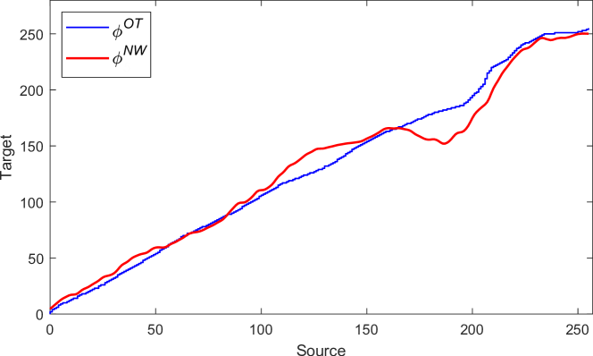
Figure 3: Illustration of the non-parametric Nadaraya-Watson mapping function ($\phi^{NW}$) that accounts for correspondences compared with the strictly increasing Optimal transport function ($\phi^{OT}$) that does not take into account the correspondences.

II-B Pipeline

II-B1 Patch correspondences

We use the same process explained in [7] to create a set of corresponding patches $\{(x_{i},y_{i})\}$ (patch size neighborhood $m\times m$, creating data dimension $d=m\times m\times 3$), where each pair corresponds to two vectors $x_{i}$ and $y_{i}$. SIFT flow motion estimation [6] is used to define the correspondences $\{(x_{i},y_{i})\}_{i=1}^{n}$. We consider likewise patches containing only colour information of a pixel neighborhood, and as an alternative definition, patches define with pixel location information in addition to colour information [7].

II-B2 Iterative Nadaraya-Watson Distribution Transfer

Our algorithm outlined in Algorithm 1 is applied to our set $\{(x_{i},y_{i})\}_{i=1}^{n}$ (input) to compute recoloured patches $\{x_{i}^{(\infty)}\}_{i=1}^{n}$. Fig. 4 illustrates several iterations $k$ of our algorithm visualised in 2D space.

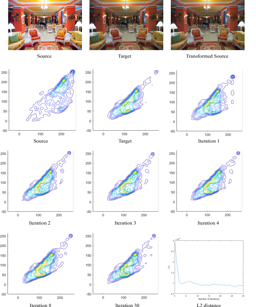
Figure 4: Example of pdf of the transferred source patches projected in 2D space (RG). The patch size chosen is $1\times 1$ and only the colour information is used $d=3$ (space RGB). The $\mathcal{L}_{2}$ distance [5] is computed at each iteration to illustrate the convergence of the original distribution to the target one by our transfer method.

II-B3 Merge recoloured candidates.

Because the same pixel is present in overlapping patches $\{x_{i}^{(\infty)}\}_{i=1}^{n}$, the average colour value from all the candidates is selected for recolouring [7, 10].

III Experimental Assessment

We provide quantitative and qualitative evaluations to validate both of our NW solutions - using colour patches only, annotated in the results as NW_c, and using colour patches with pixel location information, annotated as NW_cp. We compare our methods to different state of the art colour transfer methods noted IDT [8], PMLS [2], GPS/LCP and FGPS/LCP [9], L2 [5], PCT_OT [10] and OT_NW [7]. In these evaluations we use image pairs with similar content from an existing dataset provided by Hwang et al. [2]. The dataset includes registered pairs of images (source and target) taken with different cameras, different in-camera settings, and different illuminations and recolouring styles.

III-A Colour space and parameters settings

We use the RGB colour space and we found a patch size of $3\times 3$ captures enough of a pixel’s neighbourhood. For our NW_cp version, each pixel is represented by its 3D RGB colour values and its 2D pixel position (i.e 5D). The patches with combined colour and spatial features create a vector in 45 dimensions ($d=3\times 3\times 5=45$). For NW_c, pixel position is not accounted for, and only RGB colours are used ($d=3\times 3\times 3=27$). We experimented with different bandwidth values (cf. Eq. 2) and we found a fix value of $h=5$ gives best results.

III-B Evaluation metrics

To quantitatively assess the recolouring results, four metrics are used: peak signal to noise ratio (PSNR) [12], structural similarity index (SSIM) [13], colour image difference (CID) [14] and feature similarity index (FSIMc) [15]. These metrics are often used when considering source and target images of the same content [5, 16, 17, 2, 9]. Note that the results using PMLS were provided by the authors [2]. It has already been shown in [5] that PMLS performs better than two other more recent techniques using correspondences [18, 19], so PMLS is the one reported here with [7, 10] and [5] as algorithms that incorporate correspondences in their methodologies.

III-C Experimental Results

Figures 5, 6, 8 and 9 show detailed tables of quantitative results with means and standard errors (SE) for each metric alongside with box plots carrying a lot of statistical details. The purpose of the box plots is to visualize differences among methods and to show how close our method is to the state of the art algorithms. Figure 5 (b) and Figure 9 (b) shows PSNR and FSIMc metrics results respectively, although our method NW_cp outperforms other state of the art methods in many cases as measured by PSNR as shown in the table, by examining the box plots in both figures we see that the methods PMLS, L2, PCT_OT, OT_NW, NW_c and NW_cp are greatly overlap with each other, the median and mean values (the mean shown as red dots in the plots) are the highest among all algorithms and are very close in value and the whiskers length almost similar indicating similar data variation and consistency. Similarly, Figure 6 (b) shows SSIM box plot, we can see that NW_cp gives a closer performance to OT_NW, PMLS and L2 scoring highest values while PCT_OT greatly overlap with NW_c. In Figure 8, CID metric shows that NW_cp that combines the spatial and colour information better than NW_c in giving a similar performance with top methods. In conclusion, the quantitative metrics and the standard errors show that statistically our algorithms with Nadaraya-Watson give a comparative performance with top methods PMLS[2], L2[5], OT_NW [7] and PCT_OT [10] and outperforms the rest of the state of the art algorithms [8, 9].

Figure 10 provides qualitative results. For clarity, the results are presented in image mosaics, created by switching between the target image and the transformed source image column wise (Figure 10, top row). If the colour transfer is accurate, the resulting mosaic should look like a single image (ignoring the small motion displacement between source and target images), otherwise column differences appear.

While PMLS and PCT_OT provide equivalent results to our method in terms of metrics measures, PMLS on the one hand introduces visual artifacts if the input images are not registered correctly (Figure 7), while our method is robust to registration errors. Note that although the accuracy of the PSNR, SSIM, CID and FSIMc metrics relies on the fact that the input images are registered correctly; if this is not the case, these metrics may not accurately capture all artifacts (Figures 7 and 10). On the other hand, PCT_OT can create shadow artifacts when there are large changes between target and source images (Figure 7, in example ‘building’), while our proposed methods with and without incorporating positions information can correctly transfer colours between images that contain significant spatial differences and alleviates the shadow artifacts, as can be seen in Figure 7 with examples ’illum’, ’mart’ and ’building’. In addition, NW approach allows to create a smoother colour transfer result, and can also alleviate JPEG compression artifacts and noise (cf. Figure 7 for comparison).

IV Conclusion

We have shown how to use the Nadaraya-Watson estimator to adapt the IDT algorithm for accounting for input correspondences in registering high dimensional probability density functions. Our approach is shown to be competitive to state of the art for colour transfer in images where spaces of dimension up to 45 have been used. Future work will look into combining solution $\phi^{OT}$ and $\phi^{NW}$ to tackle semi-supervised situations where correspondences are only partially available [20, 5].

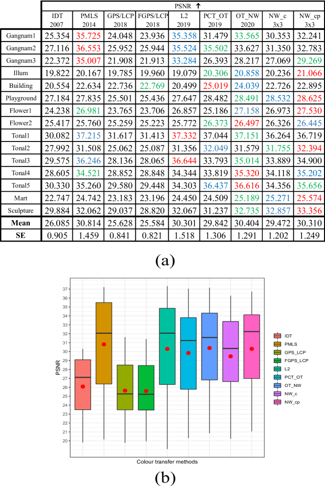
Figure 5: Metric comparison, using PSNR [12]. (a) Red, blue, and green indicate $1^{st}$, $2^{nd}$, and $3^{rd}$ best performance respectively in the table (higher values are better), (b) visualized in box plot (best viewed in colour and zoomed in).

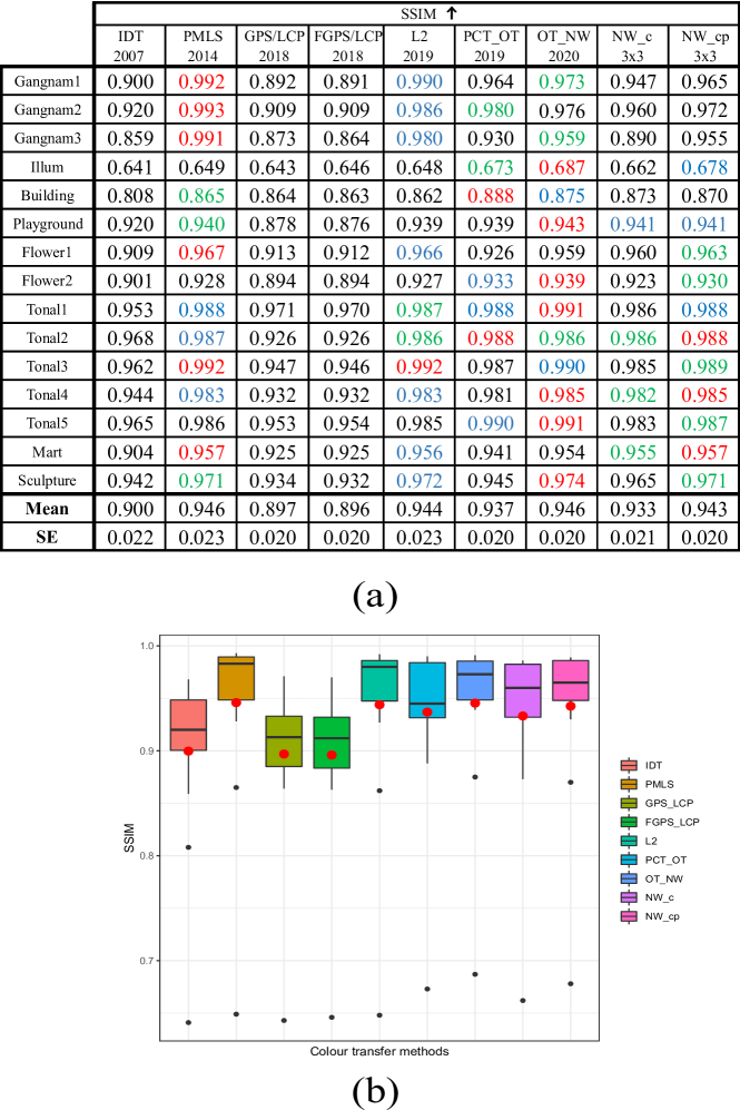
Figure 6: Metric comparison, using SSIM [13]. (a) Red, blue, and green indicate $1^{st}$, $2^{nd}$, and $3^{rd}$ best performance respectively in the table (higher values are better), (b) visualized in box plot (best viewed in colour and zoomed in).

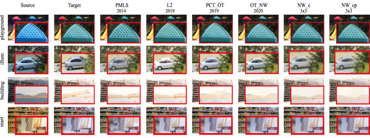
Figure 7: A close up look at some of the results generated using the top performance methods PMLS [2], L2 [5], PCT_OT [10] and OT_NW [7] and our algorithms NW_c and NW_cp (best viewed in colour and zoomed in).

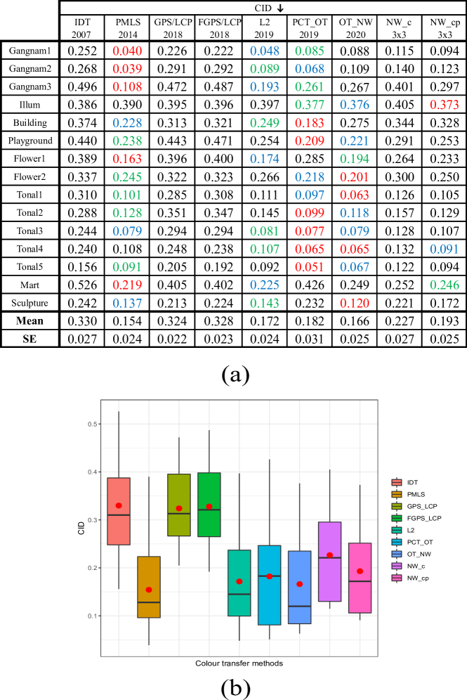
Figure 8: Metric comparison, using CID [14]. (a) Red, blue, and green indicate $1^{st}$, $2^{nd}$, and $3^{rd}$ best performance respectively in the table (lower values are better), (b) visualized in box plot (best viewed in colour and zoomed in).

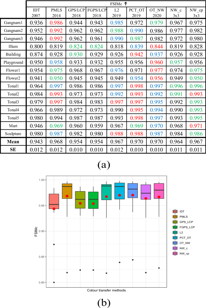
Figure 9: Metric comparison, using FSIMc [15]. (a) Red, blue, and green indicate $1^{st}$, $2^{nd}$, and $3^{rd}$ best result respectively in the table (higher values are better), (b) visualized in box plot (best viewed in colour and zoomed in).

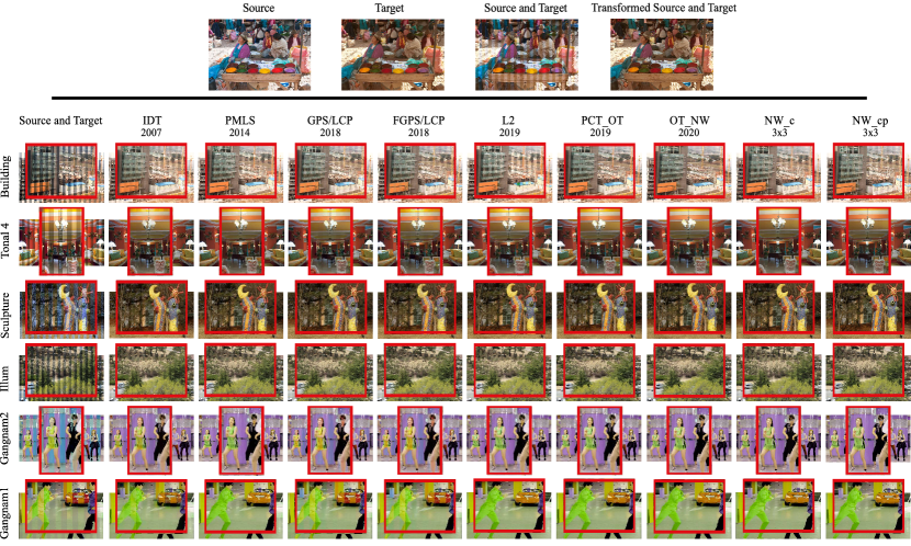
Figure 10: A close up look at some of the results generated using the IDT [8], PMLS [2], GPS/LCP and FGPS/LCP [9], L2 [5], PCT_OT [10], OT_NW [7] and our algorithms NW_c and NW_cp (best viewed in colour and zoomed in).

References

- [1] M. Brown and D. G. Lowe, “Automatic panoramic image stitching using invariant features,” International Journal of Computer Vision, vol. 74, no. 1, pp. 59–73, Aug 2007. [Online]. Available: https://doi.org/10.1007/s11263-006-0002-3
- [2] Y. Hwang, J. Lee, I. S. Kweon, and S. J. Kim, “Color transfer using probabilistic moving least squares,” in IEEE Conf. on Computer Vision and Pattern Recognition (CVPR), June 2014, pp. 3342–3349.
- [3] M. Grogan and A. Smolic, “L2 based colour correction for light field arrays,” in In Proceedings of the 16th ACM SIGGRAPH European Conference on Visual Media Production, London, UK, 17-18 December 2019.
- [4] P. Matysiak, M. Grogan, M. Le Pendu, M. Alain, E. Zerman, and A. Smolic, “High quality light field extraction and post-processing for raw plenoptic data,” IEEE Transactions on Image Processing, vol. 29, pp. 4188–4203, 2020.
- [5] M. Grogan and R. Dahyot, “L2 divergence for robust colour transfer,” Computer Vision and Image Understanding, vol. 181, pp. 39–49, 2019, https://github.com/groganma/gmm-colour-transfer.
- [6] C. Liu, J. Yuen, and A. Torralba, “Sift flow: Dense correspondence across scenes and its applications,” IEEE Transactions on Pattern Analysis and Machine Intelligence, vol. 33, no. 5, pp. 978–994, May 2011, https://people.csail.mit.edu/celiu/SIFTflow/.
- [7] H. Alghamdi and R. Dahyot, “Patch based Colour Transfer using SIFT Flow,” arXiv e-prints, p. arXiv:2005.09015, May 2020.
- [8] F. Pitié, A. C. Kokaram, and R. Dahyot, “Automated colour grading using colour distribution transfer,” Computer Vision and Image Understanding, vol. 107, no. 1, pp. 123 – 137, 2007, https://github.com/frcs/colour-transfer. [Online]. Available: http://www.sciencedirect.com/science/article/pii/S1077314206002189
- [9] F. Bellavia and C. Colombo, “Dissecting and reassembling color correction algorithms for image stitching,” IEEE Trans. Image Process., vol. 27, no. 2, pp. 735–748, Feb 2018.
- [10] H. Alghamdi, M. Grogan, and R. Dahyot, “Patch-based colour transfer with optimal transport,” in 2019 27th European Signal Processing Conference (EUSIPCO), Sep. 2019, pp. 1–5, https://github.com/leshep/PCT_OT.
- [11] S. Baker, S. Roth, D. Scharstein, M. J. Black, J. P. Lewis, and R. Szeliski, “A database and evaluation methodology for optical flow,” in 2007 IEEE 11th International Conference on Computer Vision, 2007, pp. 1–8.
- [12] D. Salomon, Data compression: the complete reference. Springer Science & Business Media, 2004.
- [13] Z. Wang, A. C. Bovik, H. R. Sheikh, and E. P. Simoncelli, “Image quality assessment: from error visibility to structural similarity,” IEEE Trans. Image Process., vol. 13, no. 4, pp. 600–612, April 2004.
- [14] J. Preiss, F. Fernandes, and P. Urban, “Color-image quality assessment: From prediction to optimization,” IEEE Trans. Image Process., vol. 23, no. 3, pp. 1366–1378, March 2014.
- [15] L. Zhang, L. Zhang, X. Mou, and D. Zhang, “Fsim: A feature similarity index for image quality assessment,” IEEE Trans. Image Process., vol. 20, no. 8, pp. 2378–2386, Aug 2011.
- [16] I. Lissner, J. Preiss, P. Urban, M. S. Lichtenauer, and P. Zolliker, “Image-difference prediction: From grayscale to color,” IEEE Trans. Image Process., vol. 22, no. 2, pp. 435–446, Feb 2013.
- [17] M. Oliveira, A. D. Sappa, and V. Santos, “A probabilistic approach for color correction in image mosaicking applications,” IEEE Trans. Image Process., vol. 24, no. 2, pp. 508–523, Feb 2015.
- [18] J. Park, Y. Tai, S. N. Sinha, and I. S. Kweon, “Efficient and robust color consistency for community photo collections,” in IEEE Conf. on Computer Vision and Pattern Recognition (CVPR), June 2016.
- [19] M. Xia, J. Y. Renping, X. M. Zhang, and J. Xiao, “Color consistency correction based on remapping optimization for image stitching,” in IEEE Int. Conf. on Computer Vision Workshops (ICCVW), Oct 2017.
- [20] M. Grogan, R. Dahyot, and A. Smolic, “User interaction for image recolouring using l2,” in Proceedings of the 14th European Conference on Visual Media Production (CVMP 2017). ACM, 2017. [Online]. Available: http://doi.acm.org/10.1145/3150165.3150171