Time discretizations of Wasserstein-Hamiltonian flows

Abstract.

We study discretizations of Hamiltonian systems on the probability density manifold equipped with the $L^{2}$-Wasserstein metric. Based on discrete optimal transport theory, several Hamiltonian systems on graph (lattice) with different weights are derived, which can be viewed as spatial discretizations to the original Hamiltonian systems. We prove the consistency and provide the approximate orders for those discretizations. By regularizing the system using Fisher information, we deduce an explicit lower bound for the density function, which guarantees that symplectic schemes can be used to discretize in time. Moreover, we show desirable long time behavior of these schemes, and demonstrate their performance on several numerical examples.

1. Introduction

In recent years, there has been a lot of interest in studying Hamiltonian systems defined on the probability space endowed with the $L^{2}$-Wasserstein metric, also known as Wasserstein manifold, and several authors have been concerned with their connections to some well-known partial differential equations (PDEs); e.g., see [1, 7, 18].

Our present study is influenced by the point of view in [4], where the authors showed that the push-forward density of a classical Hamiltonian vector field in phase space is a Hamiltonian flow on the Wasserstein manifold. To be more precise, consider a Hamiltonian system subject to initial condition $(q_{0},v_{0})$:

(1.1) $$\begin{split}dv&=-\frac{\partial H}{\partial q}(v,q),\;v(0)=v_{0},\\ dq&=\frac{\partial H}{\partial v}(v,q),\;q(0)=q_{0},\end{split}$$

where the position $q\in\mathbb{R}^{d}$, the conjugate momenta $v\in\mathbb{R}^{d}$, and the real valued Hamiltonian $H\in\mathcal{C}^{2}(\mathbb{R}^{d}\times\mathbb{R}^{d})$, $d\in\mathbb{N}^{+}$. Let $q(t)$, $v(t)$ denote the solution of (1.1). If we assume that the initial position $q_{0}$ is a random vector associated to a joint probability density $\rho_{0}$, then the density $\rho$ of $q(t)$ satisfies

(1.2) $$\begin{split}\partial_{t}\rho+\nabla\cdot(\frac{\partial H}{\partial v}\rho)&=0,\\ \partial_{t}v+\nabla v\cdot v+\nabla\cdot\frac{\partial H}{\partial q}&=0.\end{split}$$

By introducing $v=\nabla S$, one can rewrite this system as the Wasserstein-Hamiltonian system

(1.3) $$\begin{split}\partial_{t}\rho+\nabla\cdot(\frac{\partial H}{\partial v}\rho)&=0,\\ \partial_{t}S+\frac{1}{2}|\nabla S|^{2}+\frac{\partial H}{\partial q}&=C(t),\end{split}$$

where $C(t)$ is a function depending only on $t$ and $|\nabla S|^{2}=\nabla S\cdot\nabla S$.

The formulation (1.3) is remarkably powerful and general. Indeed, with different choices of the Hamiltonian $H$, the Wasserstein-Hamiltonian system (1.3) leads to differential equations arising in many different applications. For example, by taking $H(v,q)=\frac{1}{2}|v|^{2}$, one obtains the well-known geodesic equations between two densities $\rho^{0}$ and $\rho^{1}$ on the Wasserstein manifold:

(1.4) $$\begin{split}\partial_{t}\rho+\nabla\cdot({\rho}\nabla S)&=0,\\ \partial_{t}S+\frac{1}{2}|\nabla S|^{2}&=0,\end{split}$$

with $\rho(0)=\rho^{0},\rho(1)=\rho^{1}$. In the seminal paper [2], it has been proven that the solution of (1.4) is a minimizer of the following variational problem, commonly known as the Benamou-Brenier formula:

(1.5) $$\begin{split}g_{W}(\rho_{0},\rho_{1})^{2}&=\inf_{v_{t}}\{\int_{0}^{1}\langle v,v\rangle_{\rho}dt\ :\,\partial_{t}\rho+\nabla\cdot(\rho v)=0,\rho_{0}=\rho^{0},\rho_{1}=\rho^{1}\},\end{split}$$

where $\langle v,v\rangle_{\rho}:=\int_{\mathbb{R}^{d}}|v|^{2}\rho dx$. As shown in [2], the optimal value $g_{W}(\rho^{0},\rho^{1})$ is the $L^{2}$-Wasserstein distance between $\rho^{0}$ and $\rho^{1}$.

Similarly, a problem known as the Schrödinger Bridge Problem can be stated as

(1.6) $$\inf_{v}\Big{\{}\int_{0}^{1}\frac{1}{2}\langle v,v\rangle_{\rho}+\frac{\hbar^{2}}{8}I(\rho)dt\ :\,\partial_{t}\rho+\nabla\cdot(\rho v)=0,\rho_{0}=\rho^{0},\rho_{1}=\rho^{1}\Big{\}},$$

where $\hbar>0$ and $I(\rho):=\langle\nabla\log(\rho),\nabla\log(\rho)\rangle_{\rho}$ is the Fisher information. The minimizer of (1.6) satisfies the Wasserstein-Hamiltonian system (1.3) with the energy $\mathcal{H}(v,\rho)=\frac{1}{2}\int_{\mathbb{R}^{d}}|v|^{2}\rho dx-\frac{\hbar^{2}}{8}I(\rho)$ in density space. Although the Schrödinger Bridge problem is nearly 100 years old, it has recently received attention in control theory and machine learning, see [17, 10, 16].

If we change the sign of the Fisher information term in (1.6), we get

(1.7) $$\inf_{v}\Big{\{}\int_{0}^{1}\frac{1}{2}\langle v,v\rangle_{\rho}-\frac{\hbar^{2}}{8}I(\rho)dt\ :\,\partial_{t}\rho+\nabla\cdot(\rho v)=0,\rho_{0}=\rho^{0},\rho_{1}=\rho^{1}\Big{\}},$$

and this is the variational formula that Nelson used to derive the Schrödinger equation [14]. Its reformulation as Wasserstein-Hamiltonian system becomes the well known Madelung system [13].

Remark 1.1.

The Benamou-Brenier formula (1.5) has been extensively used to study Wasserstein gradient flows; e.g., see [9, 15, 18, 19]. However, unlike the variational formulations from (1.5) that use 2-point boundary values, much less is known for Wasserstein-Hamiltonian flows, hence for solutions of (1.3) for given initial values. The problem is subtle, for once because –depending on the initial condition– the solution of (1.3) may develop singularities. Moreover, there are several important properties of the Wasserstein-Hamiltonian flow, such as preservation of symplectic structure and other quantities, which make the numerical approximation of Wasserstein-Hamiltonian flows quite challenging. These considerations have motivated us to carry out the present numerical study.

To the best of our knowledge, prior to our work, there are no numerical analysis results on the full (i.e., space and time) discretization of Wasserstein-Hamiltonian systems. The way we approach this problem is by first using discrete optimal transport techniques to obtain Wasserstein-Hamiltonian systems on a graph, and view these as spatial discretizations of the original Wasserstein-Hamiltonian system. We explicitly show the consistency of the semi-discretizations, and derive lower bounds for the probability density function on different graphs. Then, we combine ideas from discrete optimal transport and symplectic integration to construct fully discrete numerical schemes for the solution of the Wasserstein-Hamiltonian system.

We would like to emphasize the crucial role of Fisher information in our study. Fisher information is widely used in many areas in statistics, physics and biology (see e.g. [6]). It appears naturally in some Wasserstein-Hamiltonian systems, such as (1.6), and it has recently been used as a regularization term in computations of optimal transport and Wasserstein gradient flows (see [12, 11] and references therein). Our analysis in this paper indicates that there are clear benefits to using Fisher information as a regularization term for the approximation of Wasserstein-Hamiltonian flows: it leads to maintaining positivity of the density function, it is conducive to having schemes that are time reversible and gauge invariant, that preserve mass and symplectic structure, and that almost preserve energy for very long times (of ${\mathcal{O}}(\tau^{-r})$, where $r$ is the order of the numerical scheme and $\tau$ is the time step-size).

This paper is organized as follows. In Section 2, we introduce the Wasserstein-Hamiltonian vector field on graphs and study its properties. In Section 3, we give an explicit lower bound of the probability density for the discrete Wasserstein-Hamiltonian flow on different graphs; the proofs of the technical results in this Section are in the Appendix at the end of the paper. Section 4 is devoted to constructing and analyzing time discretizations, and in particular we develop and analyze symplectic schemes. To compare with the results we obtain using Fisher information as regularization device, in this Section 4 we also analyze regularized schemes obtained by adding a viscosity term. Several numerical examples are given in Section 5.

2. Wasserstein-Hamiltonian Vector Field and Flow on a Finite Graph

Our goal in this Section is three-fold: to introduce a special vector field (the Wasserstein-Hamiltonian vector field) on a graph, to recognize it as a consistent spatial discretization of the PDE (1.3), and to show relevant properties of the associated flow. The latter effort is a prelude to Section 4 where also the time discretization is examined.

2.1. Wasserstein-Hamiltonian flows via discrete optimal transport

Consider a graph $G=(V,E,\Omega)$ with a node set $V=\{a_{i}\}_{i=1}^{N}$, an edge set $E$, and $\omega_{jl}\in\Omega$ are the weights of the edges: $\omega_{jl}=\omega_{lj}>0$, if there is an edge between $a_{j}$ and $a_{l}$, and $0$ otherwise. Below, we will write $(i,j)\in E$ to denote the edge in $E$ between the vertices $a_{i}$ and $a_{j}$. Finally, throughout this paper, we assume that $G$ is an undirected, strongly connected graph with no self loops or multiple edges.

Let us denote the set of discrete probabilities on the graph by ${\mathcal{P}}(G)$:

$$\mathcal{P}(G)=\{(\rho)_{j=1}^{N}\ :\,\sum_{j}\rho_{j}=1,\rho_{j}\geq 0,\;\text{for}\;j\in V\},$$

and let $\mathcal{P}_{o}(G)$ be its interior (i.e., all $\rho_{j}>0$, for $a_{j}\in V$). Let $\mathbb{V}_{j}$ be a linear potential on each node $a_{j}$, and $\mathbb{W}_{jl}=\mathbb{W}_{lj}$ an interactive potential between nodes $a_{j},a_{l}$. We let $N(i)=\{a_{j}\in V:(i,j)\in E\}$ be the adjacency set of node $a_{i}$ and $\theta_{ij}(\rho)$ be the density dependent weight on the edge $(i,j)\in E$.

Now, let us define the discrete Lagrange functional on the graph by

(2.1) $$\mathcal{L}(\rho,v)=\int_{0}^{1}\bigl{[}\frac{1}{2}\langle v,v\rangle_{\theta(\rho)}-\mathcal{V}(\rho)-\mathcal{W}(\rho)-\beta I(\rho)\bigr{]}dt,$$

where: $\rho(\cdot)\in\mathcal{P}_{o}(G)$, the vector field $v$ is a skew-symmetric matrix on $E$. And the inner product of two vector fields $u,v$ is defined by

$$\langle u,v\rangle_{\theta(\rho)}:=\frac{1}{2}\sum_{(j,l)\in E}u_{jl}v_{jl}\theta_{jl}.$$

The total linear potential $\mathcal{V}$ and interaction potential $\mathcal{W}$ are given by

$$\mathcal{V}(\rho)=\sum_{i=1}^{N}\mathbb{V}_{i}\rho_{i},\,\,\mathcal{W}(\rho)=\frac{1}{2}\sum_{i,j}\mathbb{W}_{ij}\rho_{i}\rho_{j}.$$

The parameter $\beta\geq 0$, and the discrete Fisher information is defined by

(2.2) $$I(\rho)=\frac{1}{2}\sum_{i=1}^{N}\sum_{j\in N(i)}\widetilde{\omega}_{ij}|\log(\rho_{i})-\log(\rho_{j})|^{2}\widetilde{\theta}_{ij}(\rho)$$

Remark 2.1.

Note that in (2.2), we are allowing use of edge weights $\widetilde{\omega}$ and probability weights $\widetilde{\theta}$, different from $\omega$ and $\theta$; this added flexibility may be exploited to obtain more robust space discretizations than those obtained when choosing $\widetilde{\omega}=\omega$ and $\widetilde{\theta}=\theta$, as done in [3].

The overall goal is to find the minimizer of $\mathcal{L}(\rho,v)$ subject to the constraint

$$\frac{d\rho_{i}}{dt}+div_{G}^{\theta}(\rho v)=0,$$

where the discrete divergence of the flux function $\rho v$ is defined as

$$div_{G}^{\theta}(\rho v):=-(\sum_{l\in N(j)}\sqrt{\omega_{jl}}v_{jl}\theta_{jl}).$$

As shown in [3], the critical point $(\rho,v)$ of $\mathcal{L}$ satisfies $v=\nabla_{G}S:=\sqrt{\omega_{jl}}(S_{j}-S_{l})_{(j,l)\in E}$ for some function $S$ on $V$. As a consequence, the minimization problem leads to the following discrete Wasserstein-Hamiltonian vector field on the graph $G$:

(2.3) $$\begin{split}&\frac{d\rho_{i}}{dt}+\sum_{j\in N(i)}\omega_{ij}(S_{j}-S_{i})\theta_{ij}(\rho)=0,\\ &\frac{dS_{i}}{dt}+\frac{1}{2}\sum_{j\in N(i)}\omega_{ij}(S_{i}-S_{j})^{2}\frac{\partial\theta_{ij}(\rho)}{\partial\rho_{i}}+\beta\frac{\partial I(\rho)}{\partial\rho_{i}}+\mathbb{V}_{i}+\sum_{j=1}^{N}\mathbb{W}_{ij}\rho_{j}=0.\end{split}$$

With respect to the variables $\rho$ and $S$, we can rewrite (2.3) as a Hamiltonian system with Hamiltonian function $\mathcal{H}(\rho,S)=K(S,\rho)+\mathcal{F}(\rho),$ where $K(S,\rho):=\frac{1}{2}\langle\nabla_{G}S,\nabla_{G}S\rangle_{\theta(\rho)}$ and $\mathcal{F}(\rho):=\beta I(\rho)+\mathcal{V}(\rho)+\mathcal{W}(\rho).$ In particular, if $\beta=0,$ $\mathcal{V}=0,$ and $\mathcal{W}=0$, the infimum of $\mathcal{L}(\rho,v)$ induces the Wasserstein metric on the graph, which is a discrete version of Benamou-Brenier formula:

$$W(\rho^{0},\rho^{1}):=\inf_{v}\Big{\{}\sqrt{\int_{0}^{1}\langle v,v\rangle_{\theta(\rho)}}dt\,\ :\,\frac{d\rho}{dt}+div_{G}^{\theta}(\rho v)=0,\;\rho(0)=\rho^{0},\;\rho(1)=\rho^{1}\Big{\}}.$$

The following example illustrates the importance of adding Fisher information in order to regularize the discrete Hamiltonian, so to avoid development of singularities when solving the initial value problem (2.3).

Example 2.1.

Consider a 2-point graph $G$. Let $\rho_{1}(0),\rho_{2}(0)>0$ and $S_{1}(0),S_{2}(0)$ be the corresponding initial values on the two nodes, take the weights to be constant (e.g., take them to be $1$) and let $\mathcal{F}$ be some other assigned potential on the nodes. By choosing $\theta_{12}=\theta_{21}=\frac{\rho_{1}+\rho_{2}}{2},$ (2.3) becomes

(2.4) $$\begin{split}\dot{\rho}_{1}&=-(S_{2}-S_{1})\frac{\rho_{1}+\rho_{2}}{2},\,\ \dot{\rho}_{2}=-(S_{1}-S_{2})\frac{\rho_{1}+\rho_{2}}{2},\\ \dot{S}_{1}&=-\frac{1}{4}|S_{2}-S_{1}|^{2}-\frac{\delta\mathcal{F}}{\delta\rho_{1}},\,\ \dot{S}_{2}=-\frac{1}{4}|S_{1}-S_{2}|^{2}-\frac{\delta\mathcal{F}}{\delta\rho_{2}}.\end{split}$$

Combining the above equations and using $\rho_{1}+\rho_{2}=1$, we get

$$\frac{\partial(\rho_{1}-\rho_{2})}{\partial t} =-(S_{2}-S_{1})$$

$$\frac{\partial(S_{1}-S_{2})}{\partial t} =\frac{\delta\mathcal{F}}{\delta\rho_{2}}-\frac{\delta\mathcal{F}}{\delta\rho_{1}}.$$

Now, we claim that if $\mathcal{F}$ has no singularity on the boundary of $\mathcal{P}(G)$, then positivity of $\rho_{1},\rho_{2}$ may fail. For example, taking $\mathcal{F}(\rho_{1},\rho_{2})=\frac{1}{2}\rho_{1}^{2}+\frac{1}{2}\rho_{2}^{2}$, we get $\rho_{1}(t)-\rho_{2}(t)=(\rho_{1}(0)-\rho_{2}(0))\cos(t)+(S_{1}(0)-S_{2}(0))\sin(t)$. Then, we obtain

$$\rho_{1}(t) =\frac{1}{2}+\frac{1}{2}\cos(t)(\rho_{1}(0)-\rho_{2}(0))+\frac{1}{2}\sin(t)(S_{1}(0)-S_{2}(0)),$$

$$\rho_{2}(t) =\frac{1}{2}+\frac{1}{2}\cos(t)(\rho_{2}(0)-\rho_{1}(0))+\frac{1}{2}\sin(t)(S_{2}(0)-S_{1}(0)).$$

It is clear that one of the density value can be a negative number if $|S_{1}(0)-S_{2}(0)|>1$. When taking $S_{1}(0)=S_{2}(0)$, the solution can be given in the following cases,

$$\rho_{1}(t)=\rho_{2}(t)=\frac{1}{2},\;\text{if}\;\rho_{1}(0)=\rho_{2}(0),$$

$$\rho_{1}(t)>0,\rho_{2}(t)>0,\;\text{if}\;|\rho_{1}(0)-\rho_{2}(0)|<1,$$

$$\rho_{1}(n\pi)=0,\;\text{or}\;\rho_{2}(n\pi)=0,\;\text{if}\;|\rho_{1}(0)-\rho_{2}(0)|=1.\qed$$

Let us denote with $T^{*}$ the first time for which $\lim_{t\to T^{*}}\rho_{i}(t)\leq 0$ or $\lim_{t\to T^{*}}S_{i}(t)=\infty$ for some index $i$. Following arguments similar to those in [3], we have the following result.

Proposition 2.1.

Consider (2.3) and assume that $\beta\geq 0$. Then, for any $\rho^{0}\in\mathcal{P}_{o}(G)$ and any function $S^{0}$ on $V$, there exists a unique solution of (2.3) and it satisfies the following properties (i)-(vi).

1. Mass is conserved: before time $T^{*}$,

   $$\sum_{i=1}^{N}\rho_{i}(t)=\sum_{i=1}^{N}\rho_{i}^{0}=1.$$

2. Energy is conserved: before time $T^{*}$,

   $$\mathcal{H}(\rho(t),S(t))=\mathcal{H}(\rho^{0},S^{0}).$$

3. The solution is time reversible: if $(\rho(t),S(t))$ is the solution of (2.3), then $(\rho(-t),-S(-t))$ also solves (2.3).

4. It is time transverse invariant with respect to the linear potential: if $\mathbb{V}^{\mathbb{\alpha}}=\mathbb{V}-\mathbb{\alpha}$, then $S^{\mathbb{\alpha}}=S+\mathbb{\alpha}t$ is the solution of (2.3) with potential $\mathbb{V}^{\mathbb{\alpha}}$.

5. A time invariant $\rho^{*}\in\mathcal{P}_{o}(G)$ and $S^{*}(t)=-vt$ form an interior stationary solution of (2.3) if and only if $\rho^{*}$ is the critical point of $\min_{\rho\in\mathcal{P}_{o}(G)}\mathcal{H}(\rho,S)$ and $v=\mathcal{H}(\rho^{*})+\frac{1}{2}\sum_{i=1}^{N}\sum_{j=1}^{N}\mathbb{W}_{ij}\rho^{*}_{i}\rho^{*}_{j}$.

6. Assuming that $\beta>0$ and $\widetilde{\theta}_{ij}(\rho)=0$ only if $\rho_{i}=\rho_{j}=0$, then there exists a compact set $B\subset\mathcal{P}_{o}(G)$ such that $\rho(t)\in\mathcal{P}_{o}(G)$ for all $t>0$.

Proof.

The proof of properties (i)-(v) is the same (except for the use of $\theta_{ij}$ instead of $\widetilde{\theta}_{ij}$) as that of [3, Theorem 6], thus we omit it. Here we only prove (vi). Since the coefficient of (2.3) is locally Lipschitz and $\rho^{0}\in\mathcal{P}_{o}(G)$, it is not difficult to obtain the local existence of a unique solution $(\rho(t),S(t))$ in $[0,T^{*}),$ where $T^{*}>0$ is the largest time for which $(\rho(t),S(t))$ exists and $\rho(t)\in\mathcal{P}_{o}(G)$. Thus, it suffices to show that the local solution can be extended to $T^{*}=\infty$, i.e., to show that the boundary is a repeller for $\rho(t)$. Consider $B=\{\rho\in\mathcal{P}_{o}(G)\;|\;\beta I(\rho)\leq\mathcal{H}(\rho,S)-\mathcal{F}(\rho)\}.$ It is enough to prove that $I(\rho)$ is positive infinity on the boundary. Denote $M:=\mathcal{H}(\rho,S)-\inf_{\rho\in\mathcal{P}_{o}(G)}\mathcal{F}(\rho).$ If there exists $\rho$ such that $\min_{i}\rho_{i}=0,$ and $\beta I(\rho)\leq M$, then $M\geq\frac{\beta}{2}\sum_{i}\sum_{j\in N(i)}\widetilde{\omega}_{ij}(\log(\rho_{i})-\log(\rho_{j}))^{2}\widetilde{\theta}_{ij}(\rho).$ For some $i$, we have that $\rho_{i}=0$ and that for $j\in N(i)$,

$$\beta\widetilde{\omega}_{ij}(\log(\rho_{i})-\log(\rho_{j}))^{2}\widetilde{\theta}_{ij}(\rho)\leq M.$$

This implies that $\widetilde{\theta}_{ij}(\rho)=0$ for any $j\in N(i)$. Since $G$ is connected and $V$ is a finite set, we get that $\max_{i}\rho_{i}=0$, which leads to a contradiction. ∎

From Property (vi) in Proposition 2.1, it is clear that the Fisher information term helps maintain positivity of the density function in the Wasserstein-Hamiltonian flow. This fact motivated us to regularize the discretized Wasserstein-Hamiltonian system (2.3) by adding Fisher information, and the details are discussed in Section 4.2.

There are many choices for $\theta_{ij}$ and $\widetilde{\theta}_{ij}$, as long as we require that $\widetilde{\theta}_{ij}(\rho)=0$ only if $\rho_{i}=\rho_{j}=0$, as this is needed in order to get the lower bound estimate on the density in Section 3. For $\theta_{ij}$, one can choose the upwind weight, $\theta_{ij}^{U}(\rho)=\rho_{i}$, if $S_{j}>S_{i}$, the average weight $\theta_{ij}^{A}(\rho)=\frac{\theta_{i}+\theta_{j}}{2}$, or the logarithmic weight $\theta_{ij}^{L}(\rho)=\frac{\rho_{i}-\rho_{j}}{\log(\rho_{i})-\log(\rho_{j})}$.

Remark 2.2.

The above results hold even when $G$ is not connected, in the following sense. Consider the decomposition of $G$ into disjoint connected components, and let $G=\cup_{j=1}^{l}G_{j}$. Then, relative to each subgraph $(G_{j},V^{j},\omega^{j})$, $\sum_{a_{i}\in V_{j}}\rho_{i}(t)=\sum_{a_{i}\in V_{j}}\rho_{i}^{0}$ and the properties (i)-(vi) in Proposition 2.1 also hold.

2.2. Spatial consistency for Wasserstein-Hamiltonian flows

When the graph $G$ is a lattice grid on a domain $\mathcal{M}$ in $\mathbb{R}^{d}$, (2.3) can be viewed as a consistent spatial discretization of the Wasserstein-Hamiltonian system (1.3). We show this next.

Let us consider a Hamiltonian in the density space

$$\mathcal{H}(\rho,S) =\int_{\mathcal{M}}H(x,\nabla S(x))\rho(x)d{x}$$

$$=\int_{\mathcal{M}}\frac{1}{2}|\nabla S(x)|^{2}\rho(x)dx+\mathcal{F}(\rho),$$

with the potential $\mathcal{F}(\rho)=\int_{\mathcal{M}}\mathbb{V}(x)\rho(x)dx+\frac{1}{2}\int_{\mathcal{M}}\int_{\mathcal{M}}\mathbb{W}(x,y)\rho(x)\rho(y)dxdy+\beta I(\rho),$ and $I(\rho)=\int_{\mathcal{M}}|\nabla\log(\rho)|^{2}\rho dx$. The corresponding Wasserstein-Hamiltonian vector field is

(2.5) $$\begin{split}\frac{\partial\rho}{\partial t}-\frac{\delta\mathcal{H}(\rho,S)}{\delta S}=0,\;\rho(0)=\rho^{0},\\ \frac{\partial S}{\partial t}+\frac{\delta\mathcal{H}(\rho,S)}{\delta\rho}=0,\;S(0)=S^{0}.\end{split}$$

We assume that for some $T^{*}>0$ there exists a unique smooth solution $(\rho,S)$ of (2.5) for all $t\leq T^{*}$. In the following, we show that the semi-discretization (2.3) is consistent with (2.5) for all $t\leq T^{*}$.

For simplicity, we consider the lattice graph $(G,V,\Omega)$, which is a cartesian product of $d$ one dimensional lattices: $G=G_{1}\times\cdots\times G_{d}$ with $G_{k}=(V_{k},E_{k})$, $k=1,\dots,d$. Also, let us assume that there is no interaction potential in (2.3). Denote $\omega=\frac{1}{h^{2}}$, let $i=(i_{1},i_{2},\cdots,i_{d})$ represents a point $x(i)$ in $\mathbb{R}^{d}$ and let the set of neighbors of $i$ be indicated by $N(i)$:

$$N_{k}(i)=\{(i_{1},\cdots,i_{k-1},j_{k},i_{k+1},\cdots,i_{d})\,\ :\,\ (i_{k},j_{k})\in E_{k}\}.$$

For the probability weights $\theta_{ij}(\rho)$ and $\widetilde{\theta}_{ij}(\rho)$ in (2.3), we assume that

$$\theta_{ij}(\rho)=\Theta(\rho_{i},\rho_{j}),\quad\widetilde{\theta}_{ij}(\rho)=\widetilde{\Theta}(\rho_{i},\rho_{j}),$$

where $\Theta$ and $\widetilde{\Theta}$ are symmetric $C^{1+\epsilon}$-continuous functions, $\epsilon>0$. In order to show the spatial consistency of (2.3), we further assume that

(2.6) $$\frac{\partial\Theta(x,x)}{\partial x}=\frac{1}{2},\;\Theta(x,x)=x.$$

Proposition 2.2.

Assume that $\theta$ and $\widetilde{\theta}$ satisfy (2.6). Then, the semi-discretization (2.3) is a consistent finite difference scheme for the Hamiltonian PDE (2.5).

Proof.

Let $\rho_{i}(t)=\rho(t,x(i))$, $S_{i}(t)=S(t,x(i))$ and $e_{1},\dots,e_{d}$, be the standard unit vectors. The lattice graph in the $e_{k}$ direction contains two points near $i$, i.e., $x(i)-e_{k}h$ and $x(i)+e_{k}h$, which we label $i^{+}$ and $i^{-}$ for short. At first, assume that $\Theta$ and $\widetilde{\Theta}$ are $C^{2}$ continuous. Then, by Taylor expansion at $i$ in the $e_{a}$ direction, we obtain

$$\sum_{k}\frac{1}{h^{2}}(S_{i}-S_{i^{+}})\theta_{ii^{+}}(\rho)+\sum_{k}\frac{1}{h^{2}}(S_{i}-S_{i^{-}})\theta_{ii^{-}}(\rho)$$

$$=\sum_{k}\frac{1}{h^{2}}(-\frac{\partial S}{\partial x_{k}}(x(i),t)h+\frac{1}{2}\frac{\partial^{2}S}{\partial x_{k}^{2}}(x(i),t)h^{2}+\mathcal{O}(h^{3}))(\theta_{ii}(\rho)+\frac{\partial\theta_{ii}(\rho)}{\partial\rho_{i}}\frac{\partial\rho_{i}}{\partial x_{k}}h+\mathcal{O}(h^{2}))$$

$$\quad+\sum_{k}\frac{1}{h^{2}}(\frac{\partial S}{\partial x_{k}}(x(i),t)h+\frac{1}{2}\frac{\partial^{2}S}{\partial x_{k}^{2}}(x(i),t)h^{2}+\mathcal{O}(h^{3}))(\theta_{ii}(\rho)-\frac{\partial\theta_{ii}(\rho)}{\partial\rho_{i}}\frac{\partial\rho_{i}}{\partial x_{k}}h+\mathcal{O}(h^{2}))$$

$$=\sum_{k}(\frac{\partial^{2}S}{\partial x_{k}^{2}}(x(i),t)\theta_{ii}(\rho)+2\frac{\partial S}{\partial x_{k}}(x(i),t)\frac{\partial\theta_{ii}(\rho)}{\partial\rho_{i}}\frac{\partial\rho_{i}}{\partial x_{k}})+\mathcal{O}(h^{2}).$$

Similarly,

$$-\frac{1}{2}\sum_{k}\frac{1}{h^{2}}(S_{i^{+}}-S_{i})^{2}\frac{\partial\theta_{ii^{+}}(\rho)}{\partial\rho_{i}}-\frac{1}{2}\sum_{k}\frac{1}{h^{2}}(S_{i^{-}}-S_{i})^{2}\frac{\partial\theta_{ii^{-}}(\rho)}{\partial\rho_{i}}$$

$$\quad-\beta\sum_{k}\frac{1}{h^{2}}|\log(\rho_{i^{+}})-\log(\rho_{i})|^{2}\frac{\partial\widetilde{\theta}_{ii^{+}}(\rho)}{\partial\rho_{i}}-\beta\sum_{k}\frac{1}{h^{2}}|\log(\rho_{i^{-}})-\log(\rho_{i})|^{2}\frac{\partial\widetilde{\theta}_{ii^{-}}(\rho)}{\partial\rho_{i}}$$

$$=-\frac{1}{h^{2}}\sum_{k}(\frac{\partial S}{\partial x_{k}}(x(i),t)h+\mathcal{O}(h^{2}))^{2}(\frac{\partial\theta_{ii}(\rho)}{\partial\rho_{i}}+\mathcal{O}(h))$$

$$\quad-\beta\frac{1}{h^{2}}\sum_{k}(\frac{\partial\log(\rho_{i})}{\partial x_{k}}+\mathcal{O}(h^{2}))^{2}(\frac{\partial\widetilde{\theta}_{ii}(\rho)}{\partial\rho_{i}}+\mathcal{O}(h))$$

$$=-\sum_{k}|\frac{\partial S}{\partial x_{k}}(x(i),t)|^{2}\frac{\partial\theta_{ii}(\rho)}{\partial\rho_{i}}-2\beta\frac{1}{h^{2}}\sum_{k}|\frac{\partial\log(\rho_{i})}{\partial x_{k}}|^{2}\frac{\partial\widetilde{\theta}_{ii}(\rho)}{\partial\rho_{i}}+\mathcal{O}(h^{2}).$$

Thus, if $\frac{\partial\theta_{ii}(\rho)}{\partial\rho_{i}}=\frac{\partial\widetilde{\theta}_{ii}(\rho)}{\partial\rho_{i}}=\frac{1}{2},\widetilde{\theta}_{ii}(\rho)=\theta_{ii}(\rho)=\rho_{i}$, we have

$$\frac{d\rho(t,x(i))}{dt}-\sum_{k}\frac{1}{h^{2}}(S_{i}-S_{i^{+}})\theta_{ii^{+}}(\rho)-\sum_{k}\frac{1}{h^{2}}(S_{i}-S_{i^{-}})\theta_{ii^{-}}(\rho)$$

$$=\frac{\partial\rho(t,x(i))}{\partial t}+\nabla_{x_{k}}\cdot(\nabla_{x_{k}}S(t,x(i))\rho(t,x(i)))+\mathcal{O}(h^{2}),$$

$$\frac{dS(t,x(i))}{dt}+\frac{1}{2}\sum_{k}\frac{1}{h^{2}}(S_{i^{+}}-S_{i})^{2}\frac{\partial\theta_{ii^{+}}(\rho)}{\partial\rho_{i}}+\frac{1}{2}\sum_{k}\frac{1}{h^{2}}(S_{i^{-}}-S_{i})^{2}\frac{\partial\theta_{ii^{-}}(\rho)}{\partial\rho_{i}}$$

$$+\beta\sum_{k}\frac{1}{h^{2}}|\log(\rho_{i^{+}})-\log(\rho_{i})|^{2}\frac{\partial\widetilde{\theta}_{ii^{+}}(\rho)}{\partial\rho_{i}}+\beta\sum_{k}\frac{1}{h^{2}}|\log(\rho_{i^{-}})-\log(\rho_{i})|^{2}\frac{\partial\widetilde{\theta}_{ii^{-}}(\rho)}{\partial\rho_{i}}$$

$$+V(x(i))=\frac{\partial S(t,x(i))}{\partial t}+\frac{1}{2}|\nabla_{x_{k}}S(t,x(i))|^{2}+\beta\frac{\partial I}{\partial\rho_{i}}(\rho(t,x(i)))+V(x(i))+\mathcal{O}(h^{2}),$$

which implies that (2.3) is a second order consistent semi-discretization scheme. By interpolation arguments, we complete the proof for the case that $\Theta$ and $\widetilde{\Theta}$ are $C^{1+\epsilon}$-continuous. ∎

As we show next, even if $\Theta$ and $\widetilde{\Theta}$ are not sufficiently regular, spatial consistency still holds as long as (2.6) holds. For example, one can take $\theta$ as the upwind weight, $\theta_{ij}^{U}(\rho)=\Theta^{U}(\rho_{i},\rho_{j}):=\rho_{i}$, if $S_{j}>S_{i}$, $\widetilde{\theta}$ satisfies (2.6) and $\widetilde{\Theta}$ is symmetric $C^{1+\epsilon}$-continuous .

Proposition 2.3.

Assume that $\theta=\theta^{U}$, and that $\widetilde{\theta}$ satisfies (2.6). Then (2.3) is a consistent spatial discretization of (2.5).

Proof.

We use the same notations as in the proof of Proposition 2.2. For simplicity, we assume that $S(t,x(i)+e_{k}h)\leq S(t,x(i))\leq S(t,x(i)-e_{k}h)$ and that $\widetilde{\Theta}$ is $C^{2}$ continuous. Similarly, we can show the same results for other possible configurations. By Taylor expansion, we obtain

$$\sum_{k}\frac{1}{h^{2}}(S_{i}-S_{i^{+}})\theta_{ii^{+}}(\rho)+\sum_{k}\frac{1}{h^{2}}(S_{i}-S_{i^{-}})\theta_{ii^{-}}(\rho)$$

$$=\sum_{k}\frac{1}{h^{2}}(S(t,x(i))-S(t,x(i)+e_{k}h))\rho_{i^{+}}+\sum_{k}\frac{1}{h^{2}}(S(t,x(i))-S(t,x(i)-e_{k}h))\rho_{i}$$

$$=\sum_{k}\frac{1}{h^{2}}(-\frac{\partial S}{\partial x_{k}}(x(i),t)h+\frac{1}{2}\frac{\partial^{2}S}{\partial x_{k}^{2}}(x(i),t)h^{2}+\mathcal{O}(h^{3}))\rho_{i^{+}}$$

$$\quad-\sum_{k}\frac{1}{h^{2}}(\frac{\partial S}{\partial x_{k}}(x(i),t)h+\frac{1}{2}\frac{\partial^{2}S}{\partial x_{k}^{2}}(x(i),t)h^{2}+\mathcal{O}(h^{3}))\rho_{i}$$

$$=\frac{1}{h}\frac{\partial S}{\partial x_{k}}(x(i),t)(\rho_{i^{+}}-\rho_{i})+\frac{1}{2}\frac{\partial^{2}S}{\partial x_{k}^{2}}(x(i),t)(\rho_{i^{+}}+\rho_{i})+\mathcal{O}(h)$$

$$=\nabla_{x_{k}}\cdot(\rho(t,x(i))\nabla_{x_{k}}S(t,x(i)))+\mathcal{O}(h),$$

and

$$-\frac{1}{2}\sum_{k}\frac{1}{h^{2}}(S_{i^{+}}-S_{i})^{2}\frac{\partial\theta_{ii^{+}}(\rho)}{\partial\rho_{i}}+-\frac{1}{2}\sum_{k}\frac{1}{h^{2}}(S_{i^{-}}-S_{i})^{2}\frac{\partial\theta_{ii^{-}}(\rho)}{\partial\rho_{i}}$$

$$\quad-\beta\sum_{k}\frac{1}{h^{2}}|\log(\rho_{i^{+}})-\log(\rho_{i})|^{2}\frac{\partial\widetilde{\theta}_{ii^{+}}(\rho)}{\partial\rho_{i}}-\beta\sum_{k}\frac{1}{h^{2}}|\log(\rho_{i^{-}})-\log(\rho_{i})|^{2}\frac{\partial\widetilde{\theta}_{ii^{-}}(\rho)}{\partial\rho_{i}}$$

$$=-\frac{1}{2}\sum_{k}\frac{1}{h^{2}}(S_{i^{+}}-S_{i})^{2}-\beta\sum_{k}\frac{1}{h^{2}}|\log(\rho_{i^{+}})-\log(\rho_{i})|^{2}\frac{\partial\widetilde{\theta}_{ii^{+}}(\rho)}{\partial\rho_{i}}$$

$$\quad-\beta\sum_{k}\frac{1}{h^{2}}|\log(\rho_{i^{-}})-\log(\rho_{i})|^{2}\frac{\partial\widetilde{\theta}_{ii^{-}}(\rho)}{\partial\rho_{i}}$$

$$=-\frac{1}{2h^{2}}\sum_{k}(\frac{\partial S}{\partial x_{k}}(x(i),t)h+\mathcal{O}(h^{2}))^{2}$$

$$\quad-2\beta\frac{1}{h^{2}}\sum_{k}(\frac{\partial\log(\rho_{i})}{\partial x_{k}}+\mathcal{O}(h^{2}))^{2}(\frac{\partial\widetilde{\theta}_{ii}(\rho)}{\partial\rho_{i}}+\mathcal{O}(h))$$

$$=\frac{1}{2}\sum_{k}|\frac{\partial S}{\partial x_{k}}(x(i),t)|^{2}-2\beta\frac{1}{h^{2}}\sum_{k}|\frac{\partial\log(\rho_{i})}{\partial x_{k}}|^{2}\frac{\partial\widetilde{\theta}_{ii}(\rho)}{\partial\rho_{i}}+\mathcal{O}(h).$$

Therefore, combining with the above estimate and (2.5), we have that

$$\frac{d\rho(t,x(i))}{dt}-\sum_{a}\frac{1}{h^{2}}(S_{i}-S_{i^{+}})\theta_{ii^{+}}(\rho)-\sum_{k}\frac{1}{h^{2}}(S_{i}-S_{i^{-}})\theta_{ii^{-}}(\rho)$$

$$=\frac{\partial\rho(t,x(i))}{\partial t}+\sum_{k}\nabla_{x_{k}}\cdot(\nabla_{x_{k}}S(t,x(i))\rho(t,x(i)))+\mathcal{O}(h)=\mathcal{O}(h),$$

$$\frac{dS(t,x(i))}{dt}+\frac{1}{2}\sum_{k}\frac{1}{h^{2}}(S_{i^{+}}-S_{i})^{2}\frac{\partial\theta_{ii^{+}}(\rho)}{\partial\rho_{i}}+\frac{1}{2}\sum_{k}\frac{1}{h^{2}}(S_{i^{-}}-S_{i})^{2}\frac{\partial\theta_{ii^{-}}(\rho)}{\partial\rho_{i}}$$

$$+\beta\sum_{k}\frac{1}{h^{2}}|\log(\rho_{i^{+}})-\log(\rho_{i})|^{2}\frac{\partial\widetilde{\theta}_{ii^{+}}(\rho)}{\partial\rho_{i}}+\beta\sum_{k}\frac{1}{h}|\log(\rho_{i^{-}})-\log(\rho_{i})|^{2}\frac{\partial\widetilde{\theta}_{ii^{-}}(\rho)}{\partial\rho_{i}}$$

$$+V(x(i))=\frac{\partial S(t,x(i))}{\partial t}+\sum_{k}\frac{1}{2}|\nabla_{x_{k}}S(t,x(i))|^{2}+\beta\frac{\partial I}{\partial\rho_{i}}(\rho(t,x(i)))+V(x(i))+\mathcal{O}(h).$$

∎

Remark 2.3.

In (2.3), take $\beta=\frac{\hbar^{2}}{8}>0$, a fixed number. By introducing the discrete Madelung transformation $u(t)=(u_{j}(t))_{j=1}^{N}=(\sqrt{\rho_{j}(t)}e^{\mathbf{i}\frac{S_{j}(t)}{\hbar}})_{j=1}^{N},$ (2.3) can be viewed as a nonlinear spatial approximation of the nonlinear Schrödinger equation and can be rewritten as

$$\hbar\mathbf{i}\frac{du_{j}}{dt}=-\frac{\hbar^{2}}{2}(\Delta_{G}u)_{j}+u_{j}\mathbb{V}_{j}+u_{j}\sum_{l=1}^{N}\mathbb{W}_{jl}|u_{l}|^{2},$$

where the Laplacian on the graph is defined by

$$(\Delta_{G}u)_{j} :=-u_{j}\Big{(}\frac{1}{|u_{j}|^{2}}\big{[}\sum_{l\in N(j)}\omega_{jl}(Im(\log(u_{j}))-Im(\log(u_{l})))\theta_{jl}$$

$$\quad+\sum_{l\in N(j)}\widetilde{\omega}_{jl}(Re(\log(u_{j}))-Re(\log(u_{l})))\widetilde{\theta}_{jl}\big{]}$$

$$\quad+\sum_{l\in N(j)}\omega_{jl}|Im(\log(u_{j})-\log(u_{l}))|^{2}\frac{\partial\theta_{jl}}{\partial\rho_{j}}$$

$$\quad+\sum_{l\in N(j)}\widetilde{\omega}_{jl}|Re(\log(u_{j})-\log(u_{l}))|^{2}\frac{\partial\widetilde{\theta}_{jl}}{\partial\rho_{j}}\Big{)}.$$

3. Lower bound estimate of the density

In this section, we give an explicit lower bound for the density function in (2.3) with the logarithmic weight $\widetilde{\theta}_{ij}(\rho)=\Theta^{L}(\rho_{i},\rho_{j}):=\frac{\rho_{i}-\rho_{j}}{\log(\rho_{i})-\log(\rho_{j})}$. We take two basic graphs as structures to illustrate the derivation of the lower bound. With appropriate modifications, one can obtain the lower bounds for more general graphs and different probability weights $\widetilde{\theta}.$

3.1. Lower bound for periodic nearest neighbor structure

This is the classic nearest neighbor graph, with periodic boundary conditions. Our goal is to analyze the properties of the extreme point of the Fisher information (2.2) in the present case,

(3.1) $$I(\rho)=\sum_{i=1}^{N}\widetilde{\omega}_{i,{i+1}}(\log(\rho_{i})-\log(\rho_{i+1}))(\rho_{i}-\rho_{i+1}),$$

on the set $\mathcal{P}_{o}(G)$. Denote the tangent space at $\rho\in\mathcal{P}_{o}(G)$ by $T_{\rho}\mathcal{P}_{o}(G)=\{(\sigma)_{i=1}^{N}\in\mathbb{R}^{N}|\sum_{i=1}^{N}\sigma_{i}=0\}$.

Lemma 3.1.

The function $I(\rho)$ in (3.1) is strictly convex on $\mathcal{P}_{o}(G)$ and achieves its unique minimum at the uniform distribution.

Proof.

The convexity of $I$ can be obtained by directly calculating the Hessian matrix and proving

$$\min_{\sigma\in T_{\rho}\mathcal{P}_{o}(G)}\{\sigma^{T}\text{Hess}(I(\rho))\sigma|\sigma^{T}\sigma=1\}>0.$$

Direct calculations yield that

$$\frac{\partial^{2}}{\partial\rho_{i}\rho_{j}}I(\rho)=\left\{\begin{array}[]{rcl}&\widetilde{\omega}_{i,{i+1}}\frac{1}{\rho_{i}^{2}}(\rho_{i}+\rho_{i+1})+\widetilde{\omega}_{i,i-1}\frac{1}{\rho_{i}^{2}}(\rho_{i}+\rho_{i-1})&\quad\text{for}\quad{j=i};\\ &-\widetilde{\omega}_{i,{i+1}}\frac{1}{\rho_{i}\rho_{i+1}}(\rho_{i}+\rho_{i+1})&\quad\text{for}\quad{j=i+1};\\ &-\widetilde{\omega}_{i,{i-1}}\frac{1}{\rho_{i}\rho_{i-1}}(\rho_{i}+\rho_{i-1})&\quad\text{for}\quad{j=i-1};\\ &0&\quad\text{otherwise}.\end{array}\right.$$

Thus we obtain

$$\sigma^{T}\text{Hess}I(\rho)\sigma =\sum_{i=1}^{N}(\widetilde{\omega}_{i,{i+1}}\frac{1}{\rho_{i}^{2}}(\rho_{i}+\rho_{i+1})+\widetilde{\omega}_{i,i-1}\frac{1}{\rho_{i}^{2}}(\rho_{i}+\rho_{i-1}))\sigma_{i}^{2}$$

$$\quad+\sum_{i=1}^{N}(\widetilde{\omega}_{i,{i+1}}\frac{1}{\rho_{i}\rho_{i+1}}(\rho_{i}+\rho_{i+1})\sigma_{i}\sigma_{i+1}+\widetilde{\omega}_{i,i-1}\frac{1}{\rho_{i}\rho_{i-1}}(\rho_{i}+\rho_{i-1})\sigma_{i}\sigma_{i-1})$$

$$=\sum_{i=1}^{N}\widetilde{\omega}_{i,{i+1}}(\rho_{i}+\rho_{i+1})(\frac{\sigma_{i}}{\rho_{i}}-\frac{\sigma_{i+1}}{\rho_{i+1}})^{2}\geq 0,$$

which implies the semi-positvity of $\text{Hess}(I(\rho))$. To show strict convexity, assume that there exists a unit vector $\sigma^{*}$ such that ${\sigma^{*}}^{T}\text{Hess}I(\rho)\sigma^{*}=0$. Then we have $\frac{\sigma_{1}}{\rho_{1}}=\frac{\sigma_{i}}{\rho_{i}}$ for $i=2,\cdots,N$. Since $\sigma\in T_{\rho}\mathcal{P}_{o}(G)$, then $\sum_{i=1}^{N}\sigma_{i}=\sigma_{1}(1+\sum_{i=2}^{N}\frac{\rho_{i}}{\rho_{1}})=0$. As $\rho\in\mathcal{P}_{o}(G)$, we conclude that $\sigma_{i}=0$ for all $i$, which contradicts that ${\sigma^{*}}^{T}\sigma^{*}=1$. Strict convexity implies that there is a unique minimum point on $\mathcal{P}_{o}(G)$. By using the Lagrange multiplier technique to find the minimum of $I(\rho)$ under the constraint $\sum_{i=1}^{N}{\rho_{i}}=1$ and taking the first derivative with respect to $\rho$, we obtain that the extreme point satisfies

$$\widetilde{\omega}_{i,{i+1}}\phi(\frac{\rho_{i+1}}{\rho_{i}})+\widetilde{\omega}_{i-1,{i}}\phi(\frac{\rho_{i-1}}{\rho_{i}})=\lambda,\quad\text{for}\quad i\leq N,$$

where $\phi(t)=1-t-\log(t),t\in(0,\infty)$. It is not difficult to verify that $\phi$ is strictly decreasing, convex, and $\phi(1)=0$. Then when $\lambda=0$, $\rho_{i}=\frac{1}{N}$, the extreme point $\rho_{i}=\frac{1}{N}$ is the unique minimum point such that $I(\rho)=0$. ∎

Due to convexity of $I(\rho)$, for any $C>0$ there exists $c<1/N$, such that $\inf_{0<\min_{i}(\rho_{i})\leq c}I(\rho)\geq C$. On the other hand, we also know that the exact solution preserves energy, which means that $\rho(t)\in B=\{\rho\in\mathcal{P}_{o}(G)\;|\;\beta I(\rho)\leq\mathcal{H}_{0}-\min_{\rho}(\mathcal{V}(\rho)+\mathcal{W}(\rho))\},$ where $\min_{\rho}(\mathcal{V}(\rho)+\mathcal{W}(\rho))<\infty$. Denote $M:=\mathcal{H}_{0}-\min_{\rho}(\mathcal{V}(\rho)+\mathcal{W}(\rho)).$ Thus, if we can find an upper bound $c$ such that $I(\rho)\geq\frac{M}{\beta}$, then $c$ will be a lower bound for the exact solution $\rho(t),t\geq 0$. Since

$$I(\rho)\geq\min_{i\leq N-1}\widetilde{\omega}_{i{i+1}}\sum_{i=1}^{N}(\log(\rho_{i})-\log(\rho_{i+1}))(\rho_{i}-\rho_{j}),$$

the condition that $\sum_{i=1}^{N}(\log(\rho_{i})-\log(\rho_{i+1}))(\rho_{i}-\rho_{j}))\geq\frac{1}{\min_{i\leq N-1}\widetilde{\omega}_{i{i+1}}}\frac{M}{\beta}$ ensures $I(\rho)\geq\frac{M}{\beta}$. The following result gives the anticipated lower bound, and its proof is given in the Appendix at the end, where we assume that $\widetilde{\omega}_{i,{i+1}}=1$ for simplicity.

Proposition 3.1.

Let $\min_{i}(\rho_{i}^{0})<\frac{1}{N}$. Then it holds that

$$\sup\limits_{t\geq 0}\min\limits_{i\leq N}\rho_{i}(t)\geq\min(\frac{1}{2}\min_{i}\rho_{i}^{0},\frac{1}{1+N\exp(\frac{M(N-1)([\frac{N-1}{2}]+1)}{\beta})}).$$

Proof.

See the Appendix. ∎

3.2. Lower bound for aperiodic structure

Here we consider the case of an aperiodic graph (e.g., as when we have Neumann boundary conditions), and look for the extreme points of $I(\rho)$ under the constraint $\sum_{i=1}^{N}\rho_{i}=1$. We denote the boundary point set by $V_{B}$, i.e., if $a\in V_{B}$, then there exists only one edge connecting with other points. The Fisher information term now is

(3.2) $$I(\rho)=\sum_{i=1}^{N-1}\widetilde{\omega}_{i,i+1}(\log(\rho_{i})-\log(\rho_{i+1}))(\rho_{i}-\rho_{i+1}).$$

Similarly to Lemma 3.1, we have strict convexity of $I(\rho)$.

Lemma 3.2.

$I(\rho)$ in (3.2) is strictly convex on $\mathcal{P}_{o}(G)$ and achieves its unique minimum at the uniform distribution.

The proof of the following lower bound estimate is also given in the Appendix, where for simplicity we assume that $\widetilde{\omega}_{ii+1}=1$.

Proposition 3.2.

Let $\min_{i}(\rho_{i}^{0})<\frac{1}{N}$. Assume that $\kappa\leq N-1$ is the number of nodes in $V_{B}$, $d_{max}$ is the largest distance between two nodes in $V_{B}$. Then it holds that

$$\sup_{t}\min_{i}\rho_{i}(t)\geq\min\Big{(}\frac{1}{2}\min_{i}(\rho_{i}(0)),\frac{1}{1+\kappa(d_{max}-1)\exp(2\frac{M(d_{max}-1)(N-1)}{\beta})}\Big{)},$$

where $\kappa$ is the number of nodes in $V_{B}$.

Proof.

See the Appendix. ∎

4. Time discretization of Wasserstein-Hamiltonian systems on graph

Our purpose in this section is to look at the full discretization of Wasserstein-Hamiltonian systems. In particular, we discuss the time discretization of the (regularized) spatial discretizations (2.3) and (2.5) and our main goal is to devise a symplectic discretization of the Wasserstein-Hamiltonian flow (2.3) with $\beta>0$. Then, we will discuss general regularization strategies for (2.5).

Presently, the discrete Lagrangian functional is

$$L(\rho,\dot{\rho})=\frac{1}{2}\langle\nabla_{G}S,\nabla_{G}S\rangle_{\theta_{\rho}}h-\mathcal{F}(\rho)h-\beta I(\rho)h$$

with the constraint $\frac{d\rho}{dt}+div_{G}^{\theta}(\rho\nabla_{G}S)=0$, and

$$I(\rho)=\frac{1}{2}\sum_{i=1}^{N}\sum_{j\in N(i)}\widetilde{\omega}_{ij}|\log(\rho_{i})-\log(\rho_{j})|^{2}\widetilde{\theta}_{ij}(\rho).$$

We assume that $c_{0}\leq\omega_{ij}\leq C_{0},c_{0}\leq\widetilde{\omega}_{ij}\leq C_{0}$, for some positive numbers $c_{0},C_{0}$, and that $\max_{i}\mathbb{V}_{i}+\max_{ij}\mathbb{W}_{ij}\leq M_{0}$. For simplicity, in this part we restrict consideration to $\theta_{ij}(\rho)=\theta_{ij}^{A}(\rho)=\frac{\theta_{i}+\theta_{j}}{2}$, and $\widetilde{\theta}_{ij}(\rho)=\theta_{ij}^{L}(\rho)=\frac{\rho_{i}-\rho_{j}}{\log(\rho_{i})-\log(\rho_{j})}$. Denote the maximum numbers of edges connecting to a node with $E_{max}$, and let $c$ be the uniform lower bound of $\rho$ derived in Section 3. Then, the uniform upper bound estimate of $|{S_{i}-S_{j}}|$ can be obtained in the following way.

Recall $\mathcal{H}(\rho,S)=K(S,\rho)+\mathcal{F}(\rho),$ where $K(S,\rho):=\frac{1}{2}\langle\nabla_{G}S,\nabla_{G}S\rangle_{\theta(\rho)}$ and $\mathcal{F}(\rho):=\beta I(\rho)+\mathcal{V}(\rho)+\mathcal{W}(\rho).$ Due to the conservation of $\mathcal{H}$, we have

$$K(S,\rho)+\beta I(\rho) :=\frac{1}{4}\sum_{i}\sum_{j\in N(i)}\omega_{ij}{|S_{i}(t)-S_{j}(t)|^{2}}\theta_{ij}(\rho(t))$$

$$\quad+\beta\frac{1}{2}\sum_{i,j=1}^{N}\widetilde{\omega}_{ij}(\log(\rho_{i}(t))-\log(\rho_{j}(t)))^{2}\widetilde{\theta}_{ij}(\rho(t))$$

$$\leq\mathcal{H}_{0}-\min_{i}(\mathbb{V}_{i}+\sum_{j=1}^{N}\mathbb{W}_{ij}\rho_{j})=:M.$$

Then we get

$$\max_{i}|{S_{i}-S_{j}}|^{2} \leq\frac{2M}{\min_{i,j}\omega_{ij}\min_{ij}\theta_{ij}(\rho(t))}\leq\frac{2M}{c\min_{i,j}\omega_{ij}},$$

$$\max_{i}|\log(\rho_{i})-\log(\rho_{j})|^{2} \leq\frac{M}{\min_{i,j}\widetilde{\omega}_{ij}\min_{ij}\theta_{ij}(\rho(t))}\leq\frac{M}{c\min_{i,j}\widetilde{\omega}_{ij}},$$

where $c\geq\min\Big{(}\frac{1}{2}\min_{i}\rho_{i}(0),\frac{1}{1+\kappa(d_{max}-1)\exp(2\frac{M(d_{max}-1)(N-1)}{\min_{i,j}\widetilde{\omega}_{ij}\beta})}\Big{)}$ and $\kappa$ is the number of nodes in $V_{B}$. Since $x-y\leq\log(x)-\log(y)$ for $0<y\leq x<1$, we also obtain

$$\max_{i}|\rho_{i}-\rho_{j}|^{2} \leq\frac{M}{\min_{i,j}\widetilde{\omega}_{ij}\min_{ij}\theta_{ij}(\rho(t))}\leq\frac{M}{c\min_{i,j}\widetilde{\omega}_{ij}}.$$

The Lipschitz constant of $\mathcal{H}$, $Lip(\mathcal{H})$, satisfies

$$Lip(\mathcal{H})\leq\max_{i\leq N}\Big{(}\big{|}\sum_{j\in N(i)}(S_{i}-S_{j})\omega_{ij}\theta_{ij}(\rho)\big{|},\big{|}\frac{1}{2}\sum_{j\in N(i)}\omega_{ij}(S_{i}-S_{j})^{2}\frac{\partial\theta_{ij}}{\partial\rho_{i}}+\beta\frac{\partial I}{\partial\rho_{i}}(\rho)\big{|}+M_{0}\Big{)}.$$

Then on the set $B=\{(S,\rho)|K(S,\rho)+I(\rho)\leq M\}$, we have

$$\Big{\|}\frac{\partial\mathcal{H}}{\partial S}\Big{\|}_{l^{\infty}} \leq E_{max}C_{0}\sqrt{\frac{2M}{cc_{0}}},\;\Big{\|}\frac{\partial\mathcal{H}}{\partial\rho}\Big{\|}_{l^{\infty}}\leq E_{max}C_{0}\Big{(}\frac{1}{2}\frac{M}{cc_{0}}+\beta\sqrt{\frac{M}{cc_{0}}}+\beta\frac{1}{c}+M_{0}\Big{)},$$

$$\Big{\|}\frac{\partial^{2}\mathcal{H}}{\partial S^{2}}\Big{\|}_{l^{\infty}} \leq C_{0},\;\Big{\|}\frac{\partial^{2}\mathcal{H}}{\partial\rho\partial S}\Big{\|}_{l^{\infty}}\leq\frac{1}{\sqrt{2}}C_{0}\sqrt{\frac{M}{cc_{0}}},\;\Big{\|}\frac{\partial^{2}\mathcal{H}}{\partial\rho^{2}}\Big{\|}_{l^{\infty}}\leq\beta C_{0}\big{(}\frac{1}{c}+\frac{1}{c^{2}}+M_{0}\big{)}.$$

By recursive calculations, we further get $\frac{\partial^{n}\mathcal{H}}{\partial\rho^{n}}\leq\beta C_{0}((n-2)!(\frac{1}{c})^{{n-1}}+(n-1)!(\frac{1}{c})^{n})$ for $n\geq 3$ and other partial derivatives bounded by $\frac{C_{0}}{2}$ for $n=3$ and $0$ for $n\geq 4$.

4.1. Symplectic methods

Based on the positivity of the probability density in (2.3), the constraint on $\rho$ can be rewritten as $S(t)=(-\Delta_{\rho(t)}^{\theta})^{{\dagger}}\dot{\rho}(t)$, where $(-\Delta_{\rho(t)}^{\theta})^{{\dagger}}$ is the pseudo-inverse of $-div_{G}^{\theta}(\rho\nabla_{G}(\cdot))$. Thus we have the following equivalent forms

$$\mathcal{L}(\rho,\nabla_{G}S) =\frac{1}{2}\langle\nabla_{G}S,\nabla_{G}S\rangle_{\theta_{\rho}}-\mathcal{F}(\rho)=\frac{1}{2}\langle S,\Delta_{\rho(t)}^{\theta}S\rangle h-\mathcal{F}(\rho)$$

$$=\frac{1}{2}\langle\nabla_{G}((-\Delta_{\rho(t)}^{\theta})^{{\dagger}}\dot{\rho}(t)),\nabla_{G}((-\Delta_{\rho(t)}^{\theta})^{{\dagger}}\dot{\rho}(t))\rangle_{\theta_{\rho}}-\mathcal{F}(\rho)$$

$$=\frac{1}{2}\langle(-\Delta_{\rho(t)}^{\theta})^{{\dagger}}\dot{\rho}(t)),(-\Delta_{\rho(t)}^{\theta})(-\Delta_{\rho(t)}^{\theta})^{{\dagger}}\dot{\rho}(t)\rangle-\mathcal{F}(\rho)=:L(\rho,\dot{\rho}),$$

where $\mathcal{F}(\rho)=\beta I(\rho)+\mathcal{V}(\rho)+\mathcal{W}(\rho),\beta>0.$

Consider the action integral $\mathcal{S}(\rho)=\int_{t_{0}}^{t_{1}}L(\rho(t),\dot{\rho}(t))dt$ among all curves $\rho(t)$ connecting two given probability densities $\rho(t_{0})=\rho^{0}$ and $\rho(t_{1})=\rho^{1}$, and let us consider the approximation of the action integral between $0$ and $T$, connecting $\rho(0)$ and $\rho(T)$:

$$\mathcal{S}_{\tau}(\{\rho^{n}\}_{n=0}^{N})=\sum_{n=0}^{N-1}L_{\tau}(\rho^{n},\rho^{n+1}),$$

where $L_{\tau}(\rho^{n},\rho^{n+1})$ is an approximation of $\int_{t_{n}}^{t_{n+1}}L(\rho(s),\dot{\rho}(s))ds$ with given $T=t_{N}$ and $\tau=t_{n+1}-t_{n}$. Then, letting $\frac{\partial\mathcal{S}_{\tau}}{\partial\rho^{n}}=0$, for $n=1,\cdots,N-1$, we get the discrete Euler-Lagrange equation

$$\frac{\partial L_{\tau}}{\partial x}(\rho^{n},\rho^{n+1})+\frac{\partial L_{\tau}}{\partial y}(\rho^{n-1},\rho^{n})=0,$$

where $\frac{\partial L_{\tau}}{\partial x}$ and $\frac{\partial L_{\tau}}{\partial y}$ refer to the partial derivatives with respect to the first and second argument.

By introducing the discrete momenta via the discrete Legendre transformation $p^{n}=-\frac{\partial L_{\tau}}{\partial x}(\rho^{n},\rho^{n+1})$, we can get $d\mathcal{S}_{\tau}=p^{N}d\rho^{N}-p^{0}d\rho^{0}$. $\mathcal{S}_{\tau}$ is also called symplecticity generating function. This implies the symplecticity of the map $(p^{0},\rho^{0})\to(p^{N},\rho^{N})$ (see e.g. [8, Chapter VI]). Indeed, we get

$$p^{n}=-\frac{\partial L_{\tau}}{\partial x}(\rho^{n},\rho^{n+1}),\;p^{n+1}=\frac{\partial L_{\tau}}{\partial y}(\rho^{n},\rho^{n+1}).$$

Let us consider the first time step approximation. Assume that we use some numerical integration formula, and get $L_{\tau}(\rho^{0},\rho^{1})=\tau\sum_{i=1}^{s}b_{i}L(u(c_{i}\tau),\dot{u}(c_{i}\tau)),$ where $0\leq c_{1}<\dots<c_{s}\leq 1$ and $u(t)$ is the collocation polynomial of degree $s$ with $u(0)=\rho^{0}$ and $u(\tau)=\rho^{1}$. Then we can rewrite the above approximation as

$$L_{\tau}(\rho^{0},\rho^{1})=\tau\sum_{i=1}^{s}b_{i}L(\Phi^{i},\dot{\Phi}^{i}),$$

$$\Phi^{i}=\rho^{0}+h\sum_{j=1}^{s}a_{ij}\dot{\Phi}^{j},$$

subject to the constraint $\rho_{1}=\rho_{0}+h\sum_{i=1}^{s}b_{i}\dot{\Phi}^{i}$. We assume that all the $b_{i}$ are non-zero and that their sum equals 1. By the Lagrange multiplier method, the extremum point satisfies

$$\begin{split}S^{1}&=S^{0}-\tau\sum_{i=1}^{s}b_{i}\frac{\partial\mathcal{H}(\Xi^{i},\Phi^{i})}{\partial\rho},\\ \rho^{1}&=\rho^{0}+\tau\sum_{i=1}^{s}b_{i}\frac{\partial\mathcal{H}(\Xi^{i},\Phi^{i})}{\partial S},\\ \Xi^{i}&=S^{0}-\tau\sum_{j=1}^{s}\widetilde{a}_{ij}\frac{\partial\mathcal{H}(\Xi^{j},\Phi^{j})}{\partial\rho},\\ \Phi^{i}&=\rho^{0}+\tau\sum_{j=1}^{s}a_{ij}\frac{\partial\mathcal{H}(\Xi^{j},\Phi^{j})}{\partial S}\end{split}$$

where the coefficients satisfy the condition $\widetilde{a}_{ij}b_{i}+a_{ji}b_{j}=b_{i}b_{j}$, of partitioned Runge Kutta symplectic methods for the Wasserstein-Hamiltonian system (2.3).

Example 4.1.

Symplectic Euler method ($\widetilde{a}_{ij}=1$, $a_{ji}=0$, $b_{i}=b_{j}=1$, $s=1$)

$$\rho^{n+1}_{i} =\rho^{n}_{i}+\frac{\partial\mathcal{H}(S^{n+1},\rho^{n})}{\partial S}\tau,$$

$$=\rho^{n}_{i}-\sum_{j\in N(i)}\omega_{ij}(S_{j}^{n+1}-S_{i}^{n+1})\theta_{ij}(\rho^{n})\tau$$

$$S^{n+1}_{i} =S^{n}_{i}-\frac{\partial\mathcal{H}(S^{n+1},\rho^{n})}{\partial\rho}\tau,$$

$$=S^{n}_{i}-\frac{1}{2}\sum_{j\in N(i)}\omega_{ij}(S_{i}^{n+1}-S_{j}^{n+1})^{2}\frac{\partial\theta_{ij}(\rho^{n})}{\partial\rho_{i}}\tau-\frac{\partial\mathcal{F}(\rho^{n})}{\partial\rho_{i}}\tau,$$

where $\mathcal{F}(\rho):=\beta I(\rho)+\mathcal{V}(\rho)+\mathcal{W}(\rho).$ ∎

In the following, we focus on the case of symplectic Runge–Kutta methods, i.e., $\widetilde{a}_{ij}=a_{ij}$. With minor modifications, all results hold for the partitioned Runge–Kutta symplectic methods.

Theorem 4.1.

Assume that $G=(V,E,\Omega)$ is a connected weighted graph and that $\min_{i\leq N}\rho^{0}_{i}>0$. Then the symplectic Runge–Kutta scheme (4.1) enjoys the following properties.

1. It preserves mass:

   $$\sum_{i=1}^{N}\rho_{i}^{n}=\sum_{i=1}^{N}\rho_{i}^{0}.$$

2. It preserves symplectic structure: $d\rho^{n}\wedge dS^{n}=d\rho^{0}\wedge dS^{0}$.

3. Assuming that the scheme is symmetric, then it is time reversible: if $(\rho^{n},S^{n})$ is the solution of the full discretization, then $(\rho^{-n},-S^{-n})$ is also the solution of the full discretization.

4. It is time transverse (gauge) invariant: if $\mathbb{V}^{\mathbb{\alpha}}=\mathbb{V}-\mathbb{\alpha}$, then $S^{\mathbb{\alpha}}=S+\mathbb{\alpha}t$ is the solution of the scheme with linear potential $\mathbb{V}^{\mathbb{\alpha}}$.

5. A time invariant $\rho^{*}\in\mathcal{P}_{o}(G)$ and ${S^{*}}^{n}=-vn\tau$ form an interior stationary solution of the symplectic scheme if and only if $(\rho^{*},S^{*})$ is the critical point of $\mathcal{H}(\rho,S)$ and $v=\mathcal{H}(\rho^{*},S^{*})+\frac{1}{2}\sum_{i=1}^{N}\sum_{j=1}^{N}\mathbb{W}_{ij}\rho^{*}_{i}\rho^{*}_{j}$.

6. When $\frac{M}{\beta}$ is small enough, the scheme almost preserves the Hamiltonian up to time $T=\mathcal{O}(\tau^{-r})$:

   $$\mathcal{H}(S^{n},\rho^{n})=\mathcal{H}(S^{0},\rho^{0})+\mathcal{O}(\tau^{r}),$$

   where $r$ is the order of the symplectic numerical scheme.

Proof.

Property (i) holds since this is a linear constraint. Property (ii) can be verified by using the symplecticity condition $a_{ij}b_{i}+a_{ji}b_{j}=b_{i}b_{j}$. As far as (iii), since the exact flow of the original system $\Phi(y)=\Phi(S,\rho)$ is $g$-reversible, i.e., $g\circ\Phi=\Phi^{-1}\circ g$, with $g(S,\rho)=(-S,\rho)$, then since the one-step method $\Phi_{\tau}$ is symmetric, i.e, $\Phi_{\tau}\circ\Phi_{-\tau}=I$, then $\Phi_{\tau}$ is $g$-reversible, i.e., $g\circ\Phi_{\tau}=\Phi^{-1}_{\tau}\circ g$, and (iii) holds. Property (iv) holds because $K(\rho,S)$ is an even function of $S$ and the potential is linear. To show Property (v), we only need to show that $\rho^{*}$ satisfies the Karush-Kuhn-Tucker conditions of optimality for minimization of $\min_{\rho\in\mathcal{P}_{o}(G)}\mathcal{H}(\rho)=\min_{\rho\in\mathcal{P}_{o}(G)}(\beta I(\rho)+\mathcal{V}(\rho)+\mathcal{W}(\rho))$, which is done using the Lagrange multiplier method.

We next focus on the proof of (vi). Rewrite the $r$-th order Runge–Kutta scheme as

$$y^{1} =y^{0}+\tau\sum_{i=1}^{s}b_{i}f(\tilde{y}^{i}),$$

$$\tilde{y}^{i} =y^{0}+\tau\sum_{j=1}^{s}a_{ij}f(\tilde{y}^{j}).$$

Assume that $y_{0}\in B=\{\rho\in\mathcal{P}_{o}(G)\;|\;\beta I(\rho)\leq\mathcal{H}_{0}-\min_{\rho}(\mathcal{V}(\rho)+\mathcal{W}(\rho))\}$ and let $K$ be the smallest number such that $y^{K+1}\notin B$ and for some $j\leq N$, $y^{K+1}_{N+j}=\min_{i=1}^{N}|y^{K+1}_{N+i}|=\alpha c,0<\alpha<1$. By Taylor expansion, using recursion, we have

$$|y_{N+i}(t_{K+1})-y^{K+1}_{N+i}| \leq|y_{N+i}(t_{K})-y^{K}_{N+i}|+C_{r,M,c_{0},C_{0}}(1+\beta)(\frac{1}{c^{2r+1}}+1)\tau^{r+1}$$

$$\leq K\tau C_{r,M,c_{0},C_{0}}(1+\beta)(\frac{1}{c^{2r+1}}+1)\tau^{r},$$

which implies that for $i=1,\cdots,N$,

$$y_{N+j}(t_{K+1})\leq y^{K+1}_{N+j}-K\tau C_{r,M,c_{0},C_{0}}(1+\beta)\frac{1+c^{2r+1}}{c^{2r+1}}\tau^{r}.$$

Thus, before the time $K\tau\geq\frac{c^{2r+2}}{2\tau^{r}C_{r,M,c_{0},C_{0}}(1+\beta)}(1-\alpha)$, the lower bound of the original system is preserved by the numerical scheme. After $K\tau$, we can still write the scheme until the lower bound of the density goes to $0$. The solvability of the scheme requires the classical condition, $\max\Big{(}C_{0},\frac{1}{\sqrt{2}}C_{0}\sqrt{\frac{M}{cc_{0}}},\beta C_{0}\big{(}\frac{1}{c}+\frac{1}{c^{2}}+M_{0}\big{)}\Big{)}\tau\leq\text{constant}$, where the constant only depends on the numerical method. Due to the fact that if $T=\mathcal{O}(\tau^{-r}),$ the lower bound of the density is uniformly controlled by $c$, we complete the proof of (vi) by using the Taylor expansion ot the energy. ∎

4.1.1. Backward Error Analysis

In spite of point (vi) in Theorem 4.1, symplectic methods nearly preserve the Hamiltonian for times much longer than $\mathcal{O}(\tau^{-r})$, since the backward error analysis allows for an exponentially small error between the symplectic scheme and its modified equation. To apply the backward error analysis, we need to verify that the coefficients of the equation admit an analytic extension on the complex domain, which we do next.

By choosing the principle value of the logarithm of $z$ in $\mathbb{C}/\{0\}$, denoted by $\text{Log}(z):=\log|z|+i\text{Arg}(z)$, it is known that $\text{Log}(z)$ is analytic except along the negative real axis. Since $\frac{1}{\rho_{i}}$ and $\log(\rho_{i})$ can be extended to analytic complex functions for $\rho_{i}\in\mathbb{C}/\{0\}$, we extend

$$f(S,\rho) :=(-\frac{\partial\mathcal{H}}{\partial\rho},\frac{\partial\mathcal{H}}{\partial S})$$

$$=\Big{(}-\frac{1}{4}\sum_{j\in N(i)}\omega_{ij}(S_{i}-S_{j})^{2}-\sum_{j\in N(i)}\widetilde{\omega}_{ij}(1-\frac{\rho_{j}}{\rho_{i}}-\log(\frac{\rho_{j}}{\rho_{i}})),$$

$$\qquad\frac{1}{2}\sum_{j\in N(i)}\omega_{ij}(S_{i}-S_{j})(\rho_{i}+\rho_{j})\Big{)}$$

to a complex function in $\mathbb{C}^{2n}$ such that for any $y^{0}\in B$, $f(y)$ is analytic in the neighborhood of $y^{0}$ and that there exists $R>0$ such that

$$\|f(y)\|\leq M_{c},\;\text{for}\;\|y-y^{0}\|\leq 2R.$$

This is applicable since we can choose $R\leq\frac{1}{4}{\text{dist}}(y_{0},B)$ such that

$$\min_{i=1}^{N}|y_{N+i}|=\min_{i=1}^{N}|\rho_{i}|\geq c,$$

and that

$$\|f(y)\|_{l^{\infty}} \leq E_{max}C_{0}\Big{(}\frac{1}{2}\frac{M}{cc_{0}}+\beta\sqrt{\frac{M}{cc_{0}}}+\beta\frac{1}{c}+M_{0}\Big{)}.$$

Thus, the backward error analysis is applicable in our case. We first introduce the truncated modified differential equation of (2.3) with respect to an $r$-th order numerical scheme,

(4.1) $$\dot{\widetilde{y}}=F_{\mathcal{N}}(\widetilde{y}),\;F_{\mathcal{N}}(\widetilde{y})=f(\widetilde{y})+\tau^{r}f_{r+1}(\widetilde{y})+\cdots+\tau^{N-1}f_{\mathcal{N}}(\widetilde{y})$$

with $\widetilde{y}(0)=y(0)$. It is well-known that the above modified equation is also a Hamiltonian system with the modified Hamiltonian $\widetilde{\mathcal{H}}(y)=\mathcal{H}(y)+\tau^{r}\mathcal{H}_{r+1}(y)+\dots+\tau^{N-1}\mathcal{H}_{\mathcal{N}}(y)$. According to [8, Theorem 7.2 and Theorem 7.6], we have that for the Runge-Kutta method, if $f(y)$ is analytic and $\|f(y)\|\leq M_{c}$ in the complex ball $B_{2R}(y_{0})$, then the coefficients $d_{j}$ in the Taylor expansion of the numerical method

$$\Phi_{\tau}(y)=y+\tau f(y)+\tau^{2}d_{2}(y)+\dots+\tau^{j}d_{j}(y)+\dots,$$

are analytic and satisfy $\|d_{j}(y)\|\leq C\frac{M_{c}^{j}}{R}$ in $B_{R}(y_{0}).$ If $\tau\leq{\tau_{0}}$ with $\tau_{0}\leq C\frac{R}{M_{c}}$ for some constant $C>0$, then there exists $\mathcal{N}=\mathcal{N}(\tau)$ satisfying $\tau\mathcal{N}\leq h_{0}$ such that

$$\|\Phi_{\tau}(y^{0})-\widetilde{\phi_{N,\tau}}(y^{0})\|\leq C\tau M_{c}e^{-\frac{\tau_{0}}{\tau}},$$

where $y^{1}=\Phi_{\tau}(y^{0})$ is the numerical solution and $\widetilde{\phi_{\mathcal{N},\tau}}(y^{0})$ is the exact solution of (4.1) at $t=\tau$.

As a consequence of the above results, the long-time energy conservation is obtained. Assume that the numerical solution of the symplectic method $\Phi_{\tau}(y)$ stays in the compact set $B$, then there exists $R$, $\tau_{0}$ and $N(\tau_{0})$ such that

$$|\widetilde{\mathcal{H}}(y^{n})-\widetilde{\mathcal{H}}(y^{0})|\leq n\tau M_{c}e^{-\frac{\tau_{0}}{\tau}},$$

$$|\mathcal{H}(y^{n})-\mathcal{H}(y^{0})|\leq C\frac{M_{c}^{p+1}}{R^{p}}\tau^{p},$$

Corollary 4.1.

Under the same condition of Theorem 4.1, when $\frac{M}{\beta}$ is small enough, there exists $\tau_{0}$ small enough, $C_{M}>0$, and a modified energy $\widetilde{\mathcal{H}}$, $\mathcal{O}(\tau^{r})$-close to $\mathcal{H}$, such that for any $\tau<\tau_{0}$, $n\tau<T$,

$$|\widetilde{\mathcal{H}}(S^{n},\rho^{n})-\widetilde{\mathcal{H}}(S^{0},\rho^{0})|\leq n\tau C_{M}e^{-\frac{\tau_{0}}{\tau}}.$$

4.2. Regularizations

Here we look at two instances of regularization for (2.5): one based on Fisher information, and one based on standard viscosity solution. We assume that $\mathcal{M}\subset\mathbb{R}$ is a bounded connected domain, and for simplicity restrict to (2.5) subject to periodic boundary conditions without the term $\mathcal{F}(\rho)$. The initial condition $\rho(0)>0,$ and $S(0)$, are smooth and bounded functions on $\mathcal{M}$. We remark that all the proposed scheme can be constructed similarly in other domain in $\mathbb{R}^{d}$.

4.2.1. Fisher information regularization symplectic scheme

For the system (2.5), its Lagrangian formalism is equivalent to its Hamiltonian formalism. We can directly apply the Fisher information regularization symplectic scheme (4.1) to the semi-discretization of the considered Hamiltonian PDE. We use the mid-point scheme applied to the graph generated by the central difference scheme under the periodic condition as an example of a fully discrete scheme,

(4.2) $$\begin{split}\rho^{n+1}_{i}&=\rho^{n}_{i}+\frac{\partial\mathcal{H}(S^{n+\frac{1}{2}},\rho^{n+\frac{1}{2}})}{\partial S_{i}}\tau,\\ &=\rho^{n}_{i}-\sum_{j\in N(i)}\frac{\tau}{h^{2}}(S_{j}^{n+\frac{1}{2}}-S_{i}^{n+\frac{1}{2}})\theta_{ij}(\rho^{n+\frac{1}{2}})\\ S^{n+1}_{i}&=S^{n}_{i}-\frac{\partial\mathcal{H}(S^{n+\frac{1}{2}},\rho^{n+\frac{1}{2}})}{\partial\rho_{i}}\tau,\\ &=S^{n}_{i}-\frac{1}{2}\sum_{j\in N(i)}\frac{\tau}{h^{2}}(S_{i}^{n+\frac{1}{2}}-S_{j}^{n+\frac{1}{2}})^{2}\frac{\partial\theta_{ij}}{\partial\rho_{i}}(\rho^{n+\frac{1}{2}})-\beta\frac{\partial I(\rho^{n+\frac{1}{2}})}{\partial\rho_{i}}\tau.\end{split}$$

Then all the properties in Theorem 4.1 hold. According to the priori estimate on the coefficients of discrete Hamiltonian PDEs, we have the following space-time step size restriction,

$$\tau\leq C\min\Big{(}\frac{1}{C_{0}},\frac{1}{C_{0}}\sqrt{\frac{cc_{0}}{M}},\frac{1}{C_{0}}\frac{c^{2}}{\beta(1+c+M_{0}c^{2})}\Big{)},$$

where

$$c\geq\min(\frac{1}{2}\min_{i}\rho_{i}(0),\frac{1}{1+N\exp(\frac{M(N-1)([\frac{N-1}{2}]+1)h^{2}}{\beta})}),\;\text{and}\;c_{0}=C_{0}=\frac{1}{h^{2}}.$$

If we do not add a regularization term, like Fisher information, to the numerical scheme of (2.3), then the numerical scheme may develop singularities and produce unstable behavior. The following example indicates that even the structure-preserving numerical scheme which uses the upwind weight $\theta^{U}$ without regularization will fail –at a finite step $n$– to maintain positivity for $\rho_{i}^{n}$, and will lead to blow up for $S_{i}^{n}$.

Example 4.2.

Assume that the graph has only two points. Assume that $\rho_{1}(0),\rho_{2}(0)>0$ and $S_{1}(0),S_{2}(0)$ are the corresponding initial densities and potentials of the two points. We choose $\theta_{ij}=\widetilde{\theta}_{ij}$ as the probability weight

$$\theta_{ij}(\rho)=\rho_{j},\;\text{if}\;S_{i}>S_{j},$$

$$\theta_{ij}(\rho)=\rho_{i},\;\text{if}\;S_{i}<S_{j}.$$

For simplicity, assume that $S_{1}(0)>S_{2}(0)$, $\mathcal{F}(\rho)=0$. Then the finite dimensional system becomes

$$\dot{\rho}_{1} =(S_{1}-S_{2})\rho_{2},\;\dot{\rho}_{2}=(S_{2}-S_{1})\rho_{2},$$

$$\dot{S}_{1} =0,\;\dot{S}_{2}=-\frac{1}{2}|{S_{1}-S_{2}}|^{2}.$$

Then $S_{1}-S_{2}=\frac{S_{1}(0)-S_{2}(0)}{1-\frac{1}{2}(S_{1}(0)-S_{2}(0))t)}$. Until $t<\frac{2}{S_{1}(0)-S_{2}(0)}$, $\rho_{1}$ and $\rho_{2}$ possess the strict positivity property. When $t=\frac{2}{S_{1}(0)-S_{2}(0)}$, $\rho_{1}=1,$ $\rho_{2}=0$.

4.2.2. Regularization by adding viscosity

As alternative to adding Fisher information as regularization term, a classical regularization procedure is obtained by adding numerical viscosity in order to obtain monotone schemes for $S$. For example, by introducing the numerical viscosity $\alpha_{i}(S^{n}):=\alpha(S^{n}_{i+1}-2S^{n}_{i}-S^{n}_{i-1})$, where $\alpha\in\mathbb{R}$ is used to guarantee the monotonicity of $S^{n+1}_{i}$. This is a standard way of proceeding (elliptic regularization, which we now detail and further use in the numerical tests for comparison purposes. As we will see, although adding viscosity does lead to a well defined discretization (4.3), unlike the regularization scheme (4.2), the numerical scheme (4.3) does not preserve relevant properties of the Hamiltonian system (see Theorem (4.2) below). This can be easily appreciated in the numerical tests in Section 5.

Assume that $\max_{i,n}|\frac{S^{n}_{i+1}-S^{n}_{i}}{h}|\leq R$. Then, we can choose $\alpha$ $(0<\alpha<\frac{1}{2},\alpha\geq R\frac{\tau}{h})$ such that

$$1-\frac{\tau}{h}(\frac{(S_{i+1}^{n}-S_{i}^{n})^{+}}{h}+\frac{(S_{i-1}^{n}-S_{i}^{n})^{+}}{h})-2\alpha\geq 0,$$

$$-\frac{\tau}{h}\frac{(S_{i+1}^{n}-S_{i}^{n})^{+}}{h}+\alpha\geq 0,$$

$$-\frac{\tau}{h}\frac{(S_{i-1}^{n}-S_{i}^{n})^{+}}{h}+\alpha\geq 0.$$

Doing so, we get the following scheme:

(4.3) $$\begin{split}\rho_{i}^{n+1}&=\rho_{i}^{n}+\tau(\frac{S^{n}_{i}-S^{n}_{i+1}}{h^{2}})^{+}\rho_{i+1}^{n}+\tau(\frac{S^{n}_{i}-S^{n}_{i-1}}{h^{2}})^{+}\rho_{i-1}^{n}\\ &+\tau(\frac{S^{n}_{i}-S^{n}_{i+1}}{h^{2}})^{-}\rho_{i}^{n}+\tau(\frac{S^{n}_{i}-S^{n}_{i-1}}{h^{2}})^{-}\rho_{i}^{n}\\ S_{i}^{n+1}&=S_{i}^{n}-\frac{1}{2}\tau|\frac{(S^{n}_{i}-S^{n}_{i+1})^{-}}{h}|^{2}-\frac{1}{2}\tau|\frac{(S^{n}_{i}-S^{n}_{i-1})^{-}}{h}|^{2}+\alpha_{i}(S^{n}).\end{split}$$

Let $\rho^{0}$ and $S^{0}$ be the grid function of $\rho(0)$ and $S(0)$ on the grid $G$. Then the proposed scheme (4.3) enjoys the following properties, which implies that the numerical viscosity term leads to positivity of the density function and uniform boundedness of $S.$

Theorem 4.2.

Assume that $\max_{i,n}|\frac{S^{n}_{i+1}-S^{n}_{i}}{h}|\leq R,\ \alpha\geq R\frac{\tau}{h}$. Then there exists a unique solution $(\rho_{i}^{n},S_{i}^{n})_{n}$ of (4.3) and satisfies the following properties.

1. Mass is preserved: $\sum_{i}\rho_{i}^{n}=\sum_{i}\rho_{i}^{0}$.

2. It is strictly positive: if $\min\rho_{i}^{0}>0$, then $\min\rho_{i}^{n}>0$ for any $n$.

3. If $\frac{\tau}{h}$ is sufficient small, and $\tau,h\to 0$, then $S_{i}^{n}$ converges to the viscosity solution of the Hamilton Jacobi equation.

4. It holds that $\lim\limits_{n\to\infty}S^{n}=S^{\infty}$ and $\lim\limits_{n\to\infty}\rho^{n}=\rho^{\infty}$, where $\rho^{\infty}\in\mathcal{P}_{o}(G)$.

5. It holds that

   $$\|S^{n}\|_{l^{\infty}}\leq\|S^{0}\|_{l^{\infty}},\;\|\rho^{n}\|_{l^{\infty}}\leq\max((1+R\frac{\tau}{h})^{n}\|\rho^{0}\|_{l^{\infty}},1/h).$$

Proof.

For Properties (i), (iii) and (v), we refer to [5] for their proof relative to the numerical approximation

$$S_{i}^{n+1}=S_{i}^{n}-\frac{1}{2}\tau|\frac{(S^{n}_{i+1}-S^{n}_{i})}{h}|^{2}+\alpha_{i}(S^{n}).$$

We proceed to prove (ii) and (iv).

Due to the expression of $\rho^{n+1}_{i}$, we get

$$\rho_{i}^{n+1} \geq\rho_{i}^{n}+\frac{\tau}{h}\Big{(}(\frac{S^{n}_{i}-S^{n}_{i+1}}{h})^{-}+(\frac{S^{n}_{i}-S^{n}_{i-1}}{h})^{-}\Big{)}\rho_{i}^{n}\geq(1-2R\frac{\tau}{h})\rho_{i}^{n},$$

which leads to

$$\rho_{i}^{n}\geq(1-2R\frac{\tau}{h})^{n}\rho_{i}^{0}.$$

Thus we have that $\rho_{i}^{n}\geq e^{-c_{1}\frac{\tau n}{h}}\min_{i}\rho_{i}^{0}$ for some $c_{1}>0$ and (ii) holds.

Now we are in a position to show (iv). Since $S^{n}$ is uniformly bounded with respect to $n$, there exists a sub-sequence $\{S^{n_{k}}\}_{k}$ converging to a constant $S^{\infty}$. By using the comparison principle, we get that for any $k,l,m\in\mathbb{N}^{+}$,

$$\|S^{n_{k}+m}-S^{n_{l}+m}\|_{l^{\infty}}\leq\|S^{n_{k}}-S^{n_{l}}\|_{l^{\infty}}.$$

Thus $\{S^{n_{k}+m}\}_{k}$ is a Cauchy sequence in $l^{\infty}(V\times\mathbb{N}^{+})$ and converges to the same limit $S^{\infty}$. On the other hand, one can also check that the solution of the following relation

(4.4) $$\frac{1}{2}\Big{|}\frac{(S^{\infty}_{i}-S^{\infty}_{i+1})^{-}}{h}\Big{|}^{2}+\frac{1}{2}\Big{|}\frac{(S^{\infty}_{i}-S^{\infty}_{i-1})^{-}}{h}\Big{|}^{2}+\alpha_{i}(S^{\infty})=0$$

must be $0$. Indeed, let us assume that there is a nonzero solution for (4.4). From the fact that $\alpha_{i}(S^{\infty})>0$ if $S^{\infty}_{i}-S^{\infty}_{i+1}<0$, $S^{\infty}_{i}-S^{\infty}_{i+1}<0$ and $\alpha_{i}(S^{\infty})<0$, if $S^{\infty}_{i}-S^{\infty}_{i+1}>0$, $S^{\infty}_{i}-S^{\infty}_{i+1}>0$, the nonzero solution of (4.4) should has different signs for $S^{\infty}_{i}-S^{\infty}_{i+1}$ and $S^{\infty}_{i}-S^{\infty}_{i-1}$ at each node $a_{i}$. For simplicity assume that $S^{\infty}_{i}-S^{\infty}_{i+1}<0$ and $S^{\infty}_{i}-S^{\infty}_{i-1}>0$. Now adding all the equations together, we obtain that

$$\sum_{i=1}^{N}\frac{1}{2}\Big{|}\frac{(S^{\infty}_{i}-S^{\infty}_{i+1})^{-}}{h}\Big{|}^{2}=0,$$

which contradicts the fact that $S^{\infty}_{i}-S^{\infty}_{i+1}<0$ for $i=1,\cdots,N$. Repeating this argument, it follows that for any $1\leq n\leq N$, the solution of the following relation

$$\sum_{i=1}^{n}\left[\frac{1}{2}\Big{|}\frac{(S^{\infty}_{i}-S^{\infty}_{i+1})^{-}}{h}\Big{|}^{2}+\frac{1}{2}\Big{|}\frac{(S^{\infty}_{i}-S^{\infty}_{i-1})^{-}}{h}\Big{|}^{2}+\alpha_{i}(S^{\infty})\right]=0$$

must be $0$. As a consequence, for any subsequence $\{S^{n_{k}}\}_{k}$, we have

$$\frac{S_{i}^{n_{k}+1}-S_{i}^{n_{k}}}{\tau} =-\frac{1}{2}\Big{|}\frac{(S^{n_{k}}_{i}-S^{n_{k}}_{i+1})^{-}}{h}\Big{|}^{2}-\frac{1}{2}\Big{|}\frac{(S^{n_{k}}_{i}-S^{n_{k}}_{i-1})^{-}}{h}\Big{|}^{2}+\alpha_{i}(S^{n_{k}})$$

converges to

$$\frac{1}{2}\Big{|}\frac{(S^{\infty}_{i}-S^{\infty}_{i+1})^{-}}{h}\Big{|}^{2}+\frac{1}{2}\Big{|}\frac{(S^{\infty}_{i}-S^{\infty}_{i-1})^{-}}{h}\Big{|}^{2}+\alpha_{i}(S^{\infty})=0,$$

which only possesses the unique zero solution. Since $\|\rho\|_{l^{1}}=1$, there exists a subsequence $\{\rho^{n_{k}}\}_{k}$ which converges to a density probability $\rho^{\infty}$. From (4.3) and the convergence of $S$, we are in a position to show that all the subsequence of $\{\rho^{n}\}_{n}$ converges to the same limit $\rho^{\infty}$. In the following, we show that for given $k$ sufficient large, then $\{\rho^{n_{k}+m}\}_{m}$ is a Cauchy sequence. Indeed, we have

$$\|\rho_{i}^{n_{k}+1}-\rho_{i}^{n_{k}}\|_{l^{\infty}} \leq{\tau}\|\rho_{i+1}^{n_{k}}\|_{l^{\infty}}\|\Big{(}(\frac{S^{n_{k}}_{i}-S^{n_{k}}_{i+1}}{h^{2}})^{+}-(\frac{S^{\infty}_{i}-S^{\infty}_{i+1}}{h^{2}})^{+}\Big{)}\|_{l^{\infty}}$$

$$+{\tau}\|\rho_{i+1}^{n_{k}}\|_{l^{\infty}}\|\Big{(}\frac{S^{n_{k}}_{i}-S^{n_{k}}_{i-1}}{h^{2}})^{+}-\frac{S^{\infty}_{i}-S^{\infty}_{i-1}}{h^{2}})^{+}\Big{)}\|_{l^{\infty}}$$

$$+\tau\|\rho_{i}^{n_{k}}\|_{l^{\infty}}\|\Big{(}\frac{S^{n_{k}}_{i}-S^{n_{k}}_{i+1}}{h^{2}})^{-}-(\frac{S^{\infty}_{i}-S^{\infty}_{i+1}}{h^{2}})^{-}\Big{)}\|_{l^{\infty}}$$

$$+\tau\|\rho_{i}^{n_{k}}\|_{l^{\infty}}\|\Big{(}\frac{S_{i}^{n_{k}}-S^{n_{k}}_{i-1}}{h^{2}})^{-}-(\frac{S^{\infty}_{i}-S^{\infty}_{i-1}}{h^{2}})^{-}\Big{)}\|_{l^{\infty}},$$

which, together with the uniform convergence of $S$, implies that $\rho^{n_{k}+m}$ is a Cauchy sequence and possesses the same limit $\rho^{\infty}$. ∎

5. Numerical examples

Here we show performance of the numerical schemes on several examples. All the numerical tests are performed under periodic boundary conditions in space, for given initial conditions $\rho(0)=\rho^{0}$ and $S(0)=S^{0}$, as specified below.

Example 5.1.

[Geodesic equations] This is the system (1.4):

$$\partial_{t}\rho+\nabla\cdot(\rho\nabla S)=0,$$

$$\partial_{t}S+\frac{1}{2}|\nabla S|^{2}=0.$$

We report on the results of two different strategies: the upwind scheme (4.3) with numerical viscosity, and the Fisher information regularization symplectic scheme (4.2). We choose three different initial value conditions to compare the evolution of the density function and energy. (The different behaviors of $S$ and $\nabla S$ for (4.3) and (4.2) are not of interest, since for (4.3) $S$ will always converge to a constant; see Theorem 4.2.)

In Figure 5.1, we show the behavior of (4.3) and (4.2) with initial value $\rho^{0}(x)=\frac{\exp(-10(x-0.5)^{2})}{K}$ and $S^{0}(x)=-\frac{1}{5}\log(\cosh(5(x-0.5))).$ Here $K$ is a normalization constant so that $\int_{0}^{1}\rho^{0}(x)dx=1.$ We observe that for $T<0.15$ the two scheme behave quite closely to each other and the density concentrates at the point $0.5$. But, after $T=0.15$, the density of (4.2) begins to oscillate. Here, we choose spatial step-size $h=5\times 10^{-3}$, temporal step-size $\tau=10^{-4}$, viscosity coefficient $\alpha=1/12$ for (4.3), and $\theta_{ij}(\rho)=\theta_{ij}^{U}(\rho),$ $\widetilde{\theta}_{ij}(\rho)=\theta_{ij}^{L}(\rho),$ $\beta=10^{-5}$ for (4.2). In Figure 5.2, we also plot the density functions computed by (4.2) with different schemes and different temporal and spatial step sizes, and clearly the oscillations appear to be independent of the choice of schemes and mesh sizes; this leads us to believe that the oscillations exists for the continuous system.

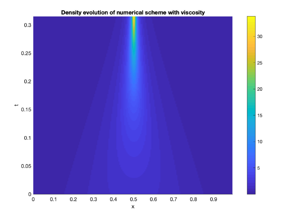
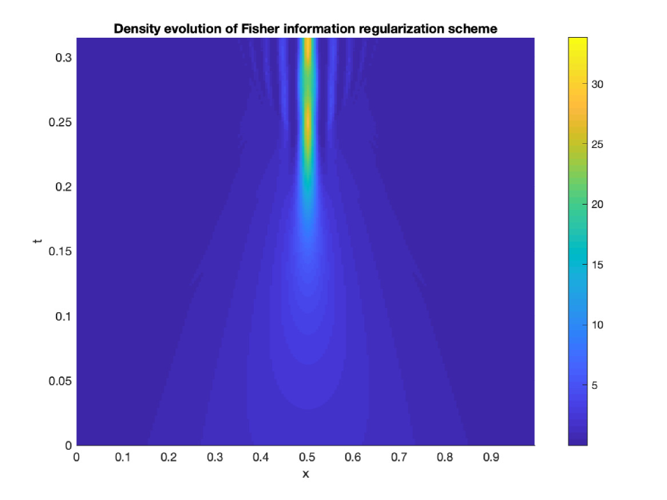
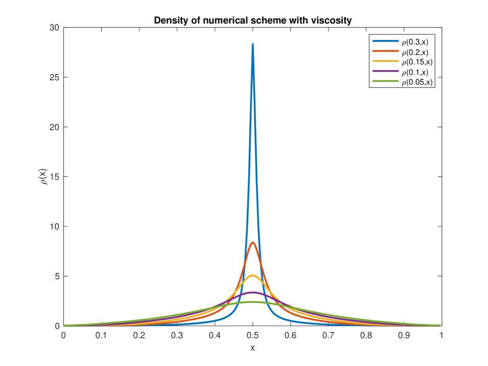
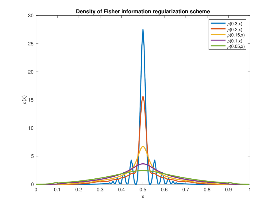
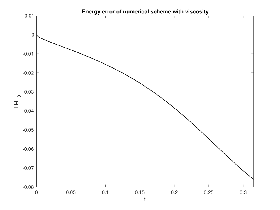
Figure 5.1. The contour plot of $\rho(t,x)$ (left), snapshots of $\rho(t,x)$ at $t=(0.3,0.2,0.15,0.1,0.05)$ (middle) and energy error before $T=0.315$ (right) for the upwind scheme (4.3) with numerical viscosity (top) and the Fisher information regularization symplectic scheme (4.2) (bottom).

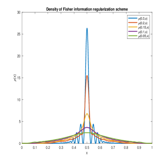
(a) Midpoint scheme

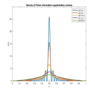
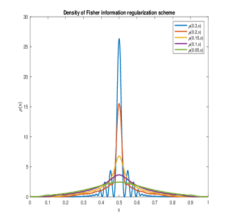
(b) Implicit Euler scheme

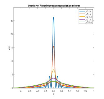
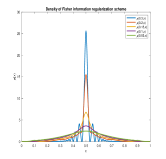
(c) Symplectic Euler scheme

Figure 5.2. In (a) and (c), there are snapshots of $\rho(t,x)$ at $t=(0.3,0.2,0.15,0.1,0.05)$ for (4.2) and (4.1) with $h=0.25\times 10^{-2},\tau=0.25\times 10^{-4}$ (left) and $h=0.125\times 10^{-2},\tau=0.2\times 10^{-4}$ (right). In (b), we show snapshots of $\rho(t,x)$ at $t=(0.3,0.2,0.15,0.1,0.05)$ for (4.2) with $h=0.25\times 10^{-2},\tau=1/3\times 10^{-4}$ (left) and $h=1/8\times 10^{-2},\tau=1/2\times 10^{-5}$ (right).

In Figure 5.3 and Firgure 5.4, we observe the same phenomenon for different initial conditions. In Figure 5.3, we take $\mathcal{M}=[0,1]$, $\rho^{0}(x)=1$ and $S^{0}(x)=-\frac{1}{5}\log(\cosh(5(x-0.5))).$ We choose spatial step-size $h=1.5\times 10^{-3}$, temporal step-size $\tau=1.3863\times 10^{-5}$, viscosity coefficient $\alpha=8\times 10^{-2}$ for (4.3), and $\theta_{ij}(\rho)=\theta_{ij}^{U}(\rho),$ $\widetilde{\theta}_{ij}(\rho)=\theta_{ij}^{L}(\rho),$ $\beta=5\times 10^{-7}$ for (4.2). In Firgure 5.4, we choose $\rho^{0}=\frac{1}{2}$, $S^{0}=\frac{1}{8}\sin(2\pi x)$, $\mathcal{M}=[0,2]$,the spatial step-size $h=10^{-2}$, temporal step-size $\tau=10^{-4}$, viscosity coefficient $\alpha=5\times 10^{-2}$ for (4.3), and $\theta_{ij}(\rho)=\theta_{ij}^{U}(\rho),$ $\widetilde{\theta}_{ij}(\rho)=\theta_{ij}^{L}(\rho),$ $\beta=10^{-4}$ for (4.2). All these numerical tests show that the Fisher information regularization scheme (4.2) preserves more structures for (2.5), such as the energy evolution and time transverse invariance, compared to the numerical scheme (4.3). Meanwhile (4.2) causes oscillatory behaviors after the singularity of (2.5) is developed.

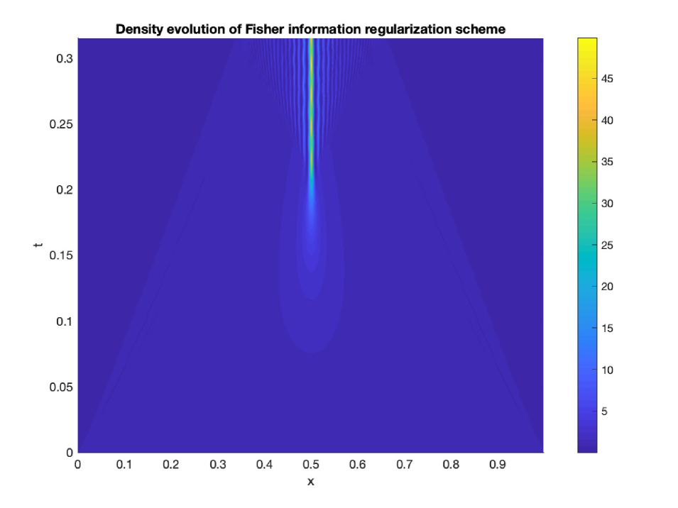
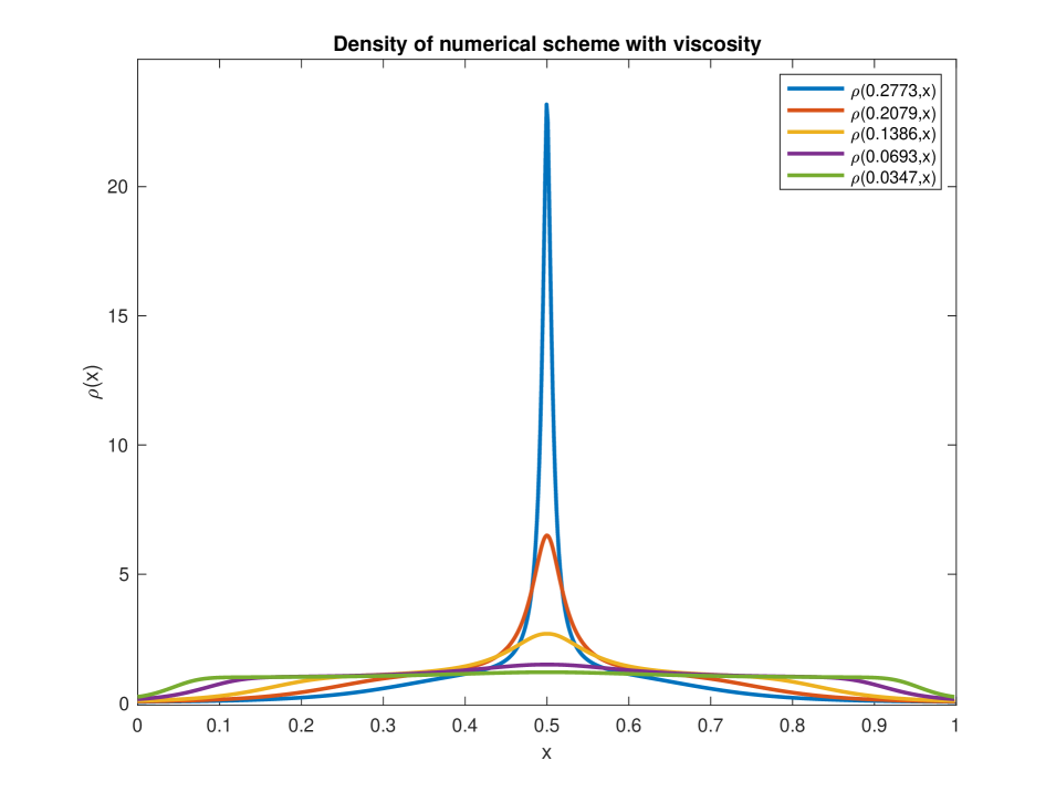
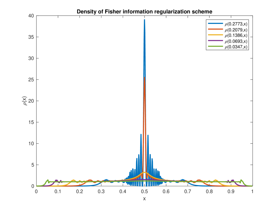
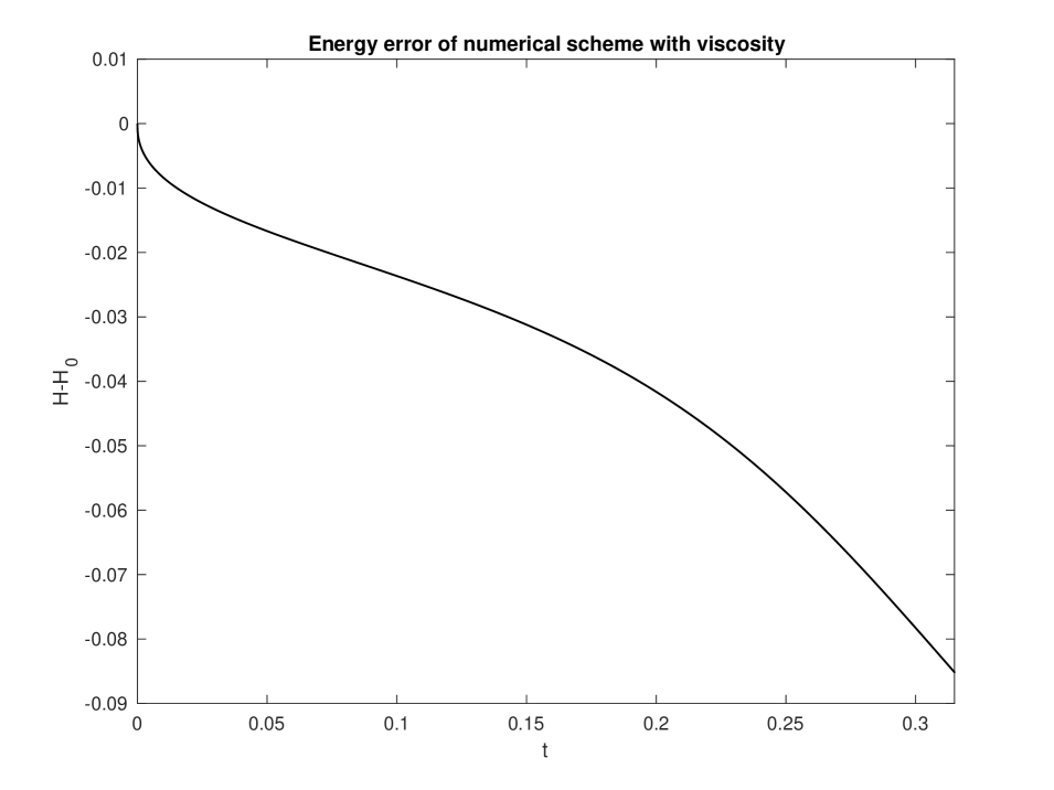
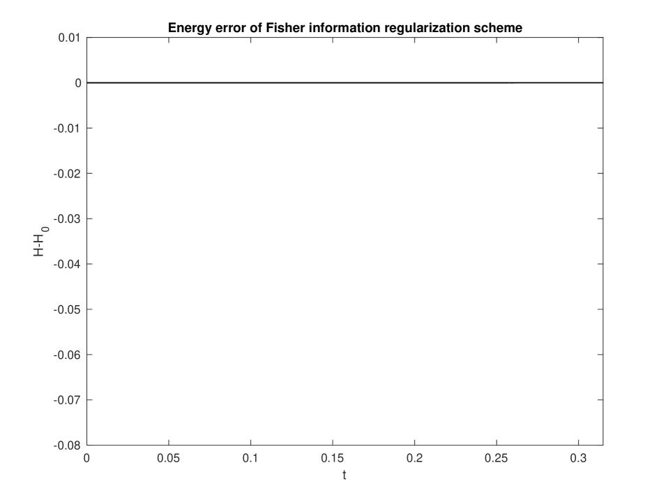
Figure 5.3. Contour plot of $\rho(t,x)$ (left), snapshots of $\rho(t,x)$ at $t=(0.2773,0.2079,0.1386,0.0693,0.0347)$ (right) and the energy error before $T=0.315$ (right) for the upwind scheme (4.3) with numerical viscosity (top) and the Fisher information regularization symplectic scheme (4.2) (bottom).

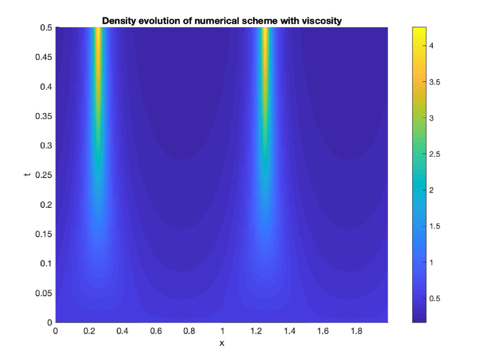
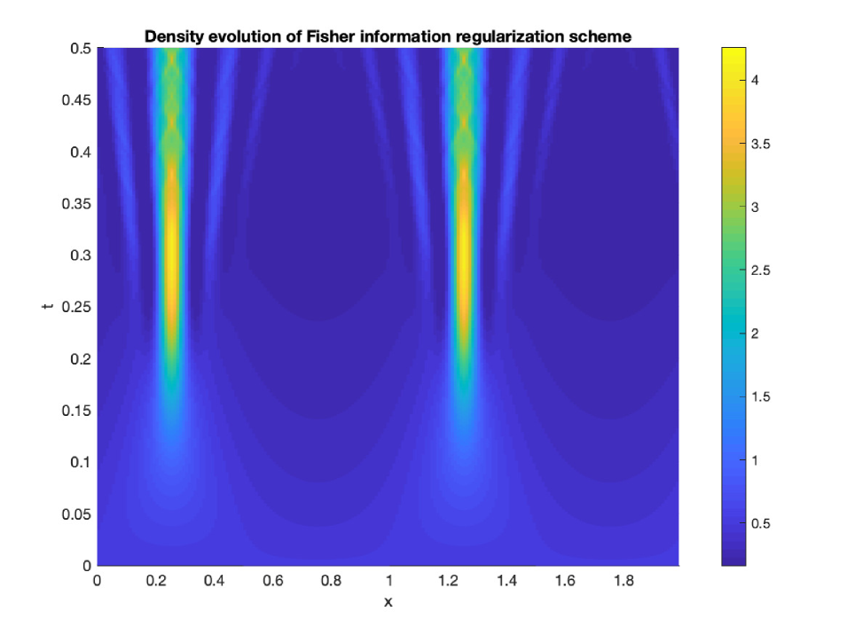
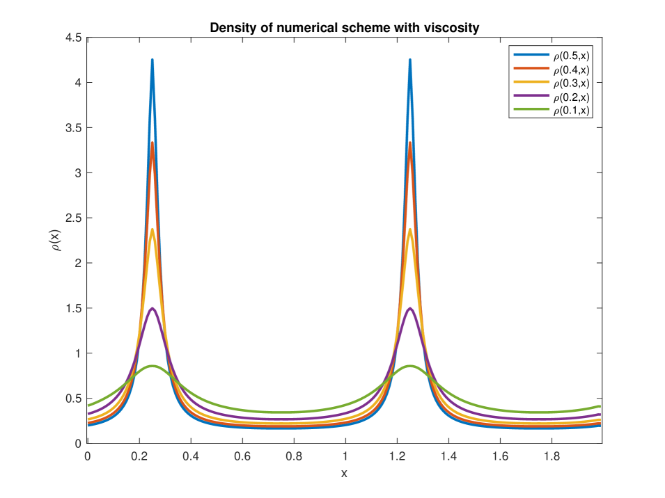
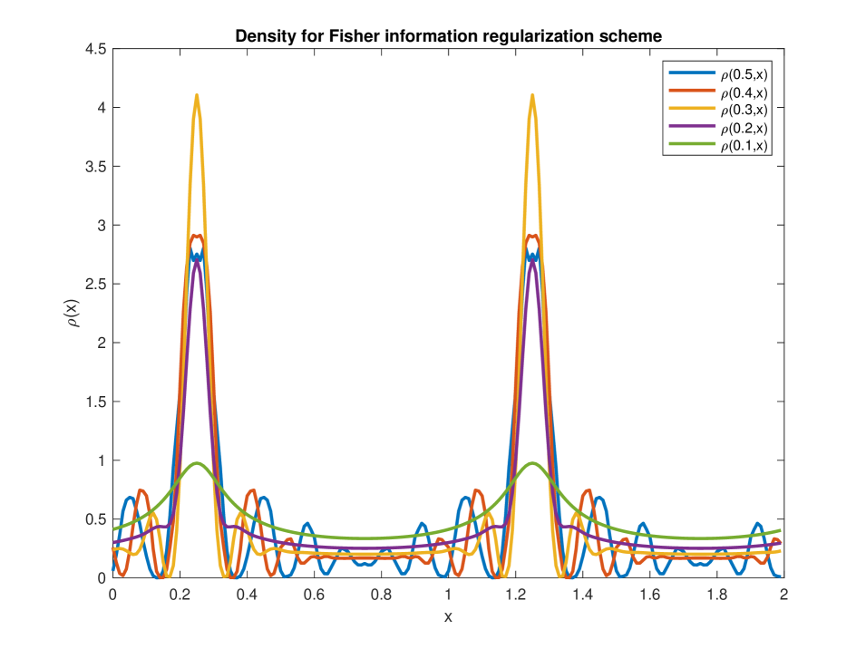
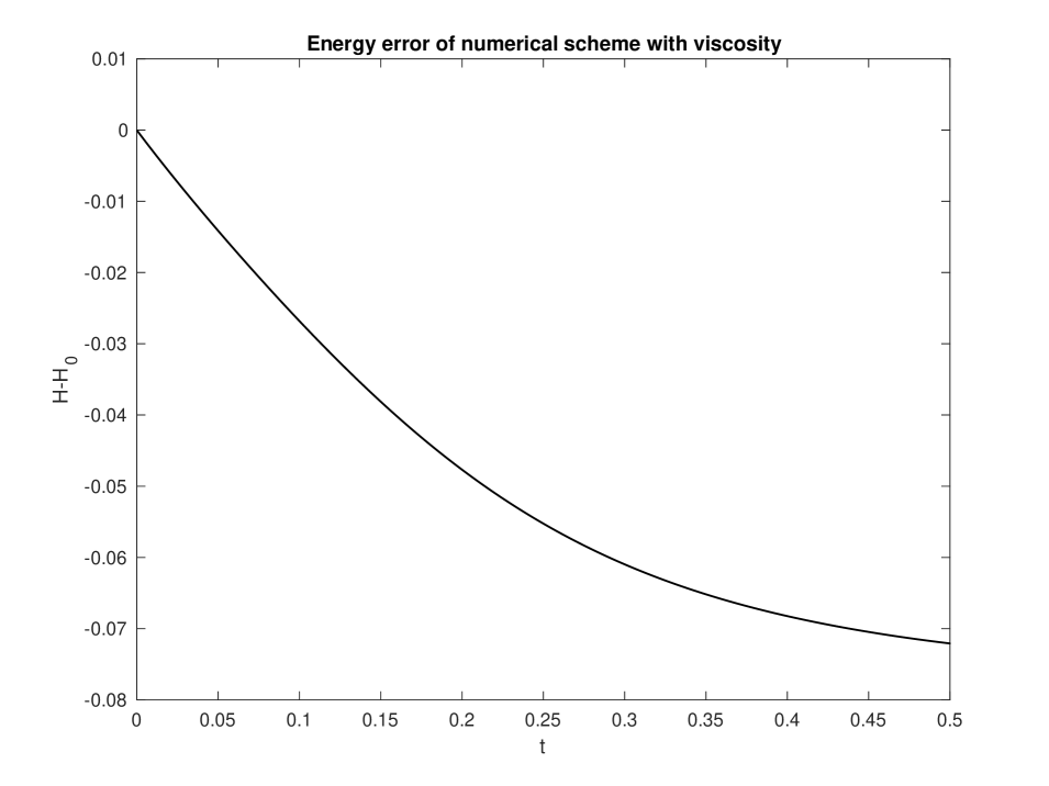
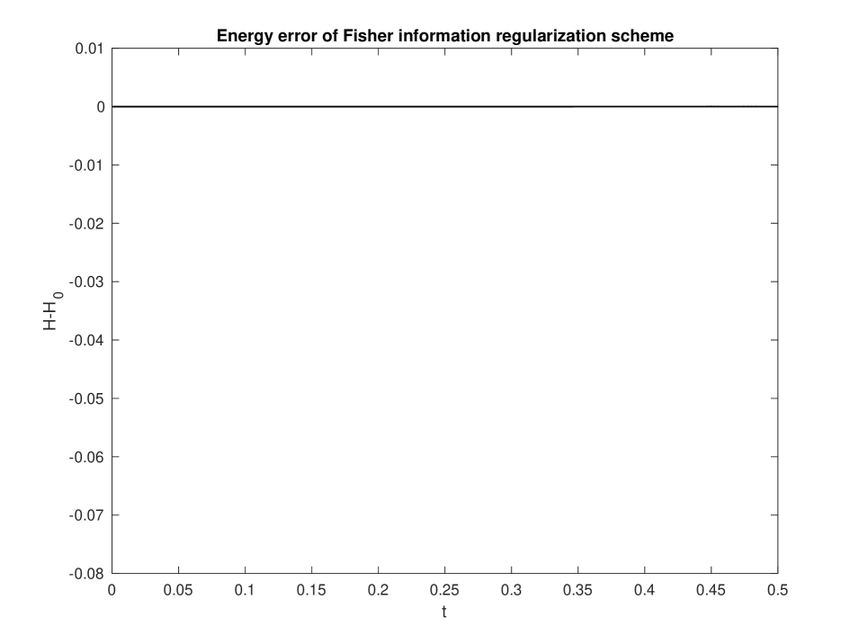
Figure 5.4. Contour plot of $\rho(t,x)$ (left), snapshots of $\rho(t,x)$ at $t=(0.5,0.4,0.3,0.2,0.1)$ (right) and the energy error before $T=0.5$ (right) for the upwind scheme (4.3) with numerical viscosity (top) and the Fisher information regularization symplectic scheme (4.2) (bottom).

Figure 5.5 shows the relationship between $\beta$ and the largest time step-size $\tau$ in (4.2) that still gives correct approximation to the solution. In this numerical test, we use $h=5\times 10^{-2},T=4,$ $\mathcal{M}=[0,1],$ $S_{0}(x)=\frac{\sin(\pi x)}{\pi}$, $\rho_{0}(x)=1$. The parameter $\beta$ is chosen as five different values, $0.005788,0.005513,0.00525,0.005,0.00476,0.00454$. From 5.5, we can see that the relationship between $\frac{H_{0}}{\beta}$ and $\tau$ is very sensitive when $\frac{H_{0}}{\beta}$ is large.

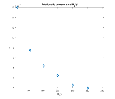
Figure 5.5. Relationship between $\frac{H_{0}}{\beta}$ and the largest time step-size $\tau$ that (4.2) with parameter $\beta=0.005788,0.005513,0.00525,0.005,0.00476,0.00454$.

Example 5.2.

[Linear Madelung system] This is the reformulation of (1.7) as Wasserstein-Hamiltonian system:

$$\partial_{t}\rho+\nabla\cdot(\rho\nabla S) =0,$$

$$\partial_{t}S+\frac{1}{2}|\nabla S|^{2}+\beta\frac{\partial}{\partial\rho}I(\rho) =0.$$

We use the scheme (4.2) for a given $\beta>0$. Figure 5.6 shows the behaviors of $\rho$ and $S$, as well as the energy evolution. Here for the evolution of $\rho$ and $S$, we choose $\beta=1$, $T=0.5,$ $\tau=10^{-3}$, $h=10^{-2},$ $S^{0}(x)=1/2\sin(2\pi x),\rho^{0}(x)=1$. We also plot the evolution of energy error $\mathcal{H}(t)-\mathcal{H}_{0}$ and mass error up to $T=400,$ which shows the good longtime behaviors of the proposed scheme.

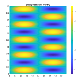
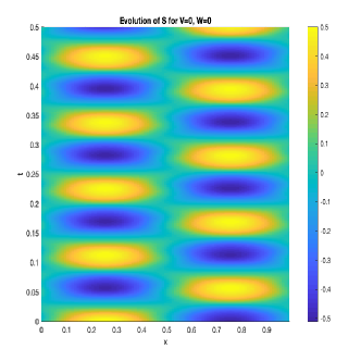
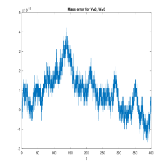
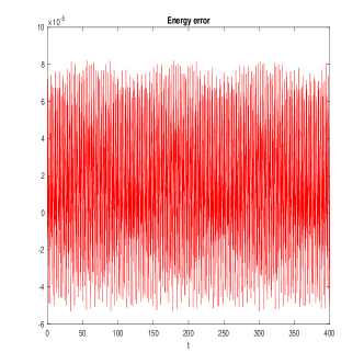
Figure 5.6. The evolutions of $\rho$ and $S$ before $T=0.5$ (a), the mass conservation law and the energy error before $T=400$ (b). Note the extremely small scales in the plots.

6. Acknowledgements

The research is partially support by Georgia Tech Mathematics Application Portal (GT-MAP) and by research grants NSF DMS-1620345. DMS-1830225, and ONR N00014-18-1-2852.

Appendix

Proof of Proposition 3.1.

It suffices to find a constant $0<c<\frac{1}{N}$ such that $\inf\limits_{0\leq\min_{i}(\rho_{i})\leq c}I(\rho)\geq\frac{M_{0}}{\beta}$. Since the graph is finite, we have that

$$\inf\limits_{0\leq\min_{i}I(\rho_{i})\leq c}I(\rho)=\min_{i\leq N}\inf\limits_{0\leq\rho_{i}\leq c}I(\rho)$$

Due to convexity of $I(\rho)$ on $0\leq\rho_{i}\leq c$ for a fixed $i\leq N$, and the fact that $I(\rho)$ approaches $\infty$ when $\rho$ approaches the boundary of $\mathcal{P}_{o}(G)$, $I(\rho)$ takes the minimum at the boundary, i.e., $\inf\limits_{0\leq\rho_{i}\leq c}I(\rho)=\inf\limits_{\rho_{i}=c}I(\rho)$ on $\mathcal{P}_{o}(G)$. Because of the periodic boundary condition, without loss of generality we can assume that $\rho_{1}=c$. By calculating the Hessian matrix of $I(\rho)$, we get for any $\sigma\neq 0$,

$$\sigma^{T}\text{Hess}I(\rho)\sigma =\sum_{i=3}^{N-1}(\frac{1}{\rho_{i}^{2}}(\rho_{i}+\rho_{i+1}+\rho_{i-1}))\sigma_{i}^{2}$$

$$\quad+\sum_{i=3}^{N-1}(\frac{1}{\rho_{i}\rho_{i+1}}(\rho_{i}+\rho_{i+1})\sigma_{i}\sigma_{i+1}+\frac{1}{\rho_{i}\rho_{i-1}}(\rho_{i}+\rho_{i-1})\sigma_{i}\sigma_{i-1})$$

$$\quad+\frac{1}{\rho_{2}^{2}}(2\rho_{i}+\rho_{3}+c)+\frac{1}{\rho_{2}\rho_{3}}(\rho_{2}+\rho_{3})$$

$$\quad+\frac{1}{\rho_{N}^{2}}(2\rho_{N}+\rho_{N-1}+c)+\frac{1}{\rho_{N}\rho_{N-1}}(\rho_{N}+\rho_{N-1})$$

$$=\sum_{i=2}^{N-1}(\rho_{i}+\rho_{i+1})(\frac{\sigma_{i}}{\rho_{i}}-\frac{\sigma_{i+1}}{\rho_{i+1}})^{2}+\frac{1}{\rho_{2}^{2}}(\rho_{2}+c)\sigma_{2}^{2}+\frac{1}{\rho_{N}^{2}}(\rho_{N}+c)\sigma_{N}^{2}>0,$$

which implies strict convexity of $I(c,\cdot)$ on $\sum_{i=2}^{N}\rho_{i}=1-c$. Using the Lagrange multiplier technique on $I(c,\rho_{2},\cdots,\rho_{N})-\lambda(\sum_{i=2}^{N}\rho_{i}-1+c)$, we get that the unique minimum point satisfies

(A.1) $$\begin{split}\phi(\frac{c}{\rho_{2}})+\phi(\frac{\rho_{3}}{\rho_{2}})&=\lambda,\\ \phi(\frac{\rho_{i-1}}{\rho_{i}})+\phi(\frac{\rho_{i+1}}{\rho_{i}})&=\lambda,\;\text{if}\;3\leq i\leq N-1,\\ \phi(\frac{\rho_{N-1}}{\rho_{N}})+\phi(\frac{c}{\rho_{N}})&=\lambda,\end{split}$$

where $\phi(t)=1-t-\log(t)$. We claim that $\rho_{N-i+1}=\rho_{i+1}$, for $i=1,\cdots,\frac{N-1}{2},$ if $N-1$ is even number. When $N-1$ is odd, we have $\rho_{N-i+1}=\rho_{i+1}$, for $i=1,\cdots,[\frac{N-1}{2}]$, where $[s]$ is the largest integer smaller than or equal to $s\in\mathbb{R}$.

To prove this claim, it suffices to show that $\rho_{2}=\rho_{N}$. Assume that $\rho_{2}>\rho_{N}$, Due to the monotonicity of $\phi$, we have $\frac{c}{\rho_{2}}<\frac{c}{\rho_{N}}$,

(A.2) $$\frac{\rho_{3}}{\rho_{2}}>\frac{\rho_{N-1}}{\rho_{N}},\frac{\rho_{4}}{\rho_{3}}>\frac{\rho_{N-2}}{\rho_{N-1}},\cdots,\frac{\rho_{i+2}}{\rho_{i+1}}>\frac{\rho_{N-i}}{\rho_{N-i+1}},\;\text{for}\;1\leq i\leq[\frac{N-1}{2}].$$

If $N-1$ is even, we obtain that

$$\phi(\frac{\rho_{\frac{N-1}{2}+2}}{\rho_{\frac{N-1}{2}+1}})<\phi(\frac{\rho_{\frac{N-1}{2}+1}}{\rho_{\frac{N-1}{2}+2}}),$$

which leads to $\frac{\rho_{\frac{N-1}{2}+1}}{\rho_{\frac{N-1}{2}+2}}<\frac{\rho_{\frac{N-1}{2}+2}}{\rho_{\frac{N-1}{2}+1}},$ i.e., $\rho_{\frac{N-1}{2}+2}>\rho_{\frac{N-1}{2}+1}.$ Thus, we can conclude from (A.2) that

$$\frac{\rho_{N}}{\rho_{2}}>\frac{\rho_{N-1}}{\rho_{3}}>\cdots>\frac{\rho_{\frac{N-1}{2}+2}}{\rho_{\frac{N-1}{2}+1}}>1,$$

which contradicts the assumption $\rho_{2}>\rho_{N}$. If $N-1$ is odd, similar arguments yield that

$$\phi(\frac{\rho_{[\frac{N-1}{2}]+2}}{\rho_{[\frac{N-1}{2}]+1}})<\phi(\frac{\rho_{[\frac{N-1}{2}]+2}}{\rho_{[\frac{N-1}{2}]+3}}),$$

which implies that $\rho_{[\frac{N-1}{2}]+3}>\rho_{[\frac{N-1}{2}]+1}$. Thus from (A.2), we have that

$$\frac{\rho_{N}}{\rho_{2}}>\frac{\rho_{N-1}}{\rho_{3}}>\cdots>\frac{\rho_{[\frac{N-1}{2}]+3}}{\rho_{[\frac{N-1}{2}]+1}}>1,$$

which contradicts the assumption $\rho_{2}>\rho_{N}$. One can show that $\rho_{2}<\rho_{N}$ is also impossible by the same arguments. As a consequence, $\rho_{2}=\rho_{N}$. By further using (A.1), we immediately get $\rho_{N-i+1}=\rho_{i+1}$, for $i=1,\cdots,[\frac{N-1}{2}].$

Now, we are going to show that the extreme point possesses the monotonicity along the path starting from $a_{1}$. Indeed, $\rho_{i}$ is increasing when $d_{1,i+1}$ is increasing for $i\leq[\frac{N-1}{2}]$ if $N$ is odd and for $i\leq[\frac{N-1}{2}]+1$ if $N$ is even. We use Figure A.1 to illustrate these two different cases.

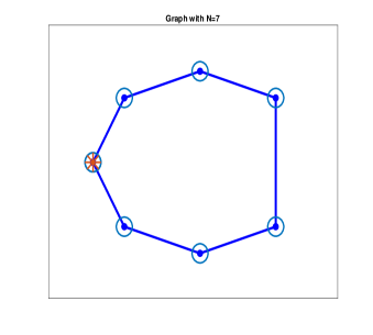
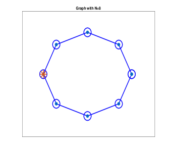
Figure A.1. The picture of the graph with $N=7$ (left) and with $N=8$ (right), where the red node represents $v_{1}$.

Step 1: $\lambda>0$. Since $\lambda=0$ if and only if $\rho_{i}=\frac{1}{N}$, then $I(\rho)=0$ which contradicts the fact that $\inf_{\rho}I(\rho)>0$. Assume that $\lambda<0$. Then (A.1), together with the symmetry $\rho_{i+1}=\rho_{N-i+1},i=1,\cdots,[\frac{N-1}{2}]$, implies that when $N-1$ is even, it holds that

(A.3) $$\begin{split}\phi(\frac{\rho_{i-1}}{\rho_{i}})+\phi(\frac{\rho_{i+1}}{\rho_{i}})&=\lambda,\;\text{if}\;2\leq i\leq\frac{N-1}{2}-1,\\ \phi(\frac{\rho_{\frac{N-1}{2}}}{\rho_{\frac{N-1}{2}+1}})&=\lambda.\end{split}$$

Since $\lambda<0$, we obtain that

$$\rho_{\frac{N-1}{2}+1}<{\rho_{\frac{N-1}{2}}}<\cdots<\rho_{2}<\rho_{1}=c,$$

which contradicts the fact that $\sum_{i=2}^{N}\rho_{i}=1-c$. When $N-1$ is odd, then (A.1) and symmetry of $\rho_{i}$ imply that

(A.4) $$\begin{split}\phi(\frac{\rho_{i-1}}{\rho_{i}})+\phi(\frac{\rho_{i+1}}{\rho_{i}})&=\lambda,\;\text{if}\;2\leq i\leq[\frac{N-1}{2}],\\ 2\phi(\frac{\rho_{[\frac{N-1}{2}]+1}}{\rho_{[\frac{N-1}{2}]+2}})&=\lambda.\end{split}$$

Then we get $\rho_{[\frac{N-1}{2}]+2}<{\rho_{[\frac{N-1}{2}]+1}}<\cdots<\rho_{2}<\rho_{1}=c,$ which is also not possible. Thus it holds that $\lambda>0$. This indicates that

$$\rho_{[\frac{N-1}{2}]+2}>{\rho_{[\frac{N-1}{2}]+1}}>\cdots>\rho_{2}>\rho_{1}=c.$$

Step 2: $\frac{\rho_{i+1}}{\rho_{i}}$ is strictly decreasing. If $N-1$ is even, $\frac{\rho_{i+1}}{\rho_{i}}$ is strictly decreasing for $1\leq i\leq[\frac{N-1}{2}]$. According to (A.3), it holds that

$$\phi(\frac{\rho_{\frac{N-1}{2}-1}}{\rho_{\frac{N-1}{2}}}) =\lambda-\phi(\frac{\rho_{\frac{N-1}{2}+1}}{\rho_{\frac{N-1}{2}}})=\phi(\frac{\rho_{\frac{N-1}{2}}}{\rho_{\frac{N-1}{2}+1}})-\phi(\frac{\rho_{\frac{N-1}{2}+1}}{\rho_{\frac{N-1}{2}}}),$$

$$\phi(\frac{\rho_{\frac{N-1}{2}-i-1}}{\rho_{\frac{N-1}{2}-i}}) =\lambda-\phi(\frac{\rho_{\frac{N-1}{2}-i+1}}{\rho_{\frac{N-1}{2}-i}})=\phi(\frac{\rho_{\frac{N-1}{2}-i}}{\rho_{\frac{N-1}{2}-i+1}})-\phi(\frac{\rho_{\frac{N-1}{2}-i+1}}{\rho_{\frac{N-1}{2}-i}})+\phi(\frac{\rho_{\frac{N-1}{2}-i+2}}{\rho_{\frac{N-1}{2}-i+1}}),$$

where $i=1,\cdots,\frac{N-5}{2}$. The monotonicity of $\rho_{i}$, $i\leq\frac{N-1}{2}$, together with $\lambda>0$, leads to

$$\phi(\frac{\rho_{\frac{N-1}{2}-i-1}}{\rho_{\frac{N-1}{2}-i}}) >\phi(\frac{\rho_{\frac{N-1}{2}-i}}{\rho_{\frac{N-1}{2}-i+1}}),\;\text{for}\;i=0,\cdots,\frac{N-5}{2}.$$

If $N-1$ is odd, $\frac{\rho_{i+1}}{\rho_{i}}$ is strictly decreasing for $1\leq i\leq[\frac{N-1}{2}]+1$. From (A.4), it follows that

$$\phi(\frac{\rho_{[\frac{N-1}{2}]}}{\rho_{[\frac{N-1}{2}]+1}}) =\lambda-\phi(\frac{\rho_{[\frac{N-1}{2}]+2}}{\rho_{[\frac{N-1}{2}]+1}})=2\phi(\frac{\rho_{[\frac{N-1}{2}]+1}}{\rho_{\frac{[N-1}{2}]+2}})-\phi(\frac{\rho_{[\frac{N-1}{2}]+2}}{\rho_{[\frac{N-1}{2}]+1}}),$$

$$\phi(\frac{\rho_{[\frac{N-1}{2}]-i-1}}{\rho_{[\frac{N-1}{2}]-i}}) =\lambda-\phi(\frac{\rho_{[\frac{N-1}{2}]-i+1}}{\rho_{[\frac{N-1}{2}]-i}})=\phi(\frac{\rho_{[\frac{N-1}{2}]-i}}{\rho_{[\frac{N-1}{2}]-i+1}})-\phi(\frac{\rho_{[\frac{N-1}{2}]-i+1}}{\rho_{[\frac{N-1}{2}]-i}})+\phi(\frac{\rho_{[\frac{N-1}{2}]-i+2}}{\rho_{[\frac{N-1}{2}]-i+1}}),$$

where $i=0,\cdots,[\frac{N-1}{2}]+1$. From the monotonicity of $\phi$, it follows that $\frac{\rho_{i+1}}{\rho_{i}}$ is strictly decreasing for $1\leq i\leq[\frac{N-1}{2}]$.

Step 3: Lower bound for $\frac{\rho_{i+1}}{\rho_{i}},i=1,\cdots,[\frac{N-1}{2}].$ We first deal with the case that $N-1$ is even. Due to monotonicity of $\frac{\rho_{i+1}}{\rho_{i}}$, its minimum is $k:=\frac{\rho_{[\frac{N-1}{2}]+1}}{\rho_{[\frac{N-1}{2}]}}$. Since $\sum_{i}\rho_{i}=1$, we have

$$c+2\sum_{i=2}^{[\frac{N-1}{2}]}\rho_{i} =c(1+2\sum_{i=2}^{[\frac{N-1}{2}]}\frac{\rho_{i}}{c})=1.$$

To find a lower bound of $\frac{\rho_{i+1}}{\rho_{i}}$, it suffices to find an upper bound such that

$$1+\sum_{i=2}^{[\frac{N-1}{2}]}k^{i-1}=\frac{k^{[\frac{N-1}{2}]}-1}{k-1}<\frac{1+c}{2c}.$$

Let $k\leq(\frac{1-c}{2c[\frac{N-1}{2}]})^{\frac{1}{[\frac{N-1}{2}]}}$. Then it holds that

$$\sum_{i=2}^{[\frac{N-1}{2}]+1}k^{i-1}\leq[\frac{N-1}{2}]k^{[\frac{N-1}{2}]}\leq\frac{1-c}{2c}.$$

Finally, we get that

$$\inf_{\rho_{1}=c}I(\rho) =2\sum_{i=1}^{[\frac{N-1}{2}]}(\log(\rho_{i}^{*})-\log(\rho_{i+1}^{*}))(\rho_{i}^{*}-\rho_{i+1}^{*})$$

$$\geq{2}(\log(\frac{\rho_{[\frac{N-1}{2}]+1}^{*}}{\rho_{[\frac{N-1}{2}]}^{*}}))(\rho_{[\frac{N-1}{2}]+1}^{*}-c).$$

Since there exists at least $\rho_{j}^{*},j\leq N$ such that $\rho_{j}^{*}>\frac{1-c}{N-1}$, thus it holds that

(A.5) $$\inf_{\rho_{1}=c}I(\rho) \geq{2}(\log(\frac{\rho_{[\frac{N-1}{2}]+1}^{*}}{\rho_{[\frac{N-1}{2}]}^{*}}))(\frac{1-c}{N-1}-c)\geq 2\log(k)(\frac{1-c}{N-1}-c)\geq\frac{M}{\beta}.$$

Now, we are able to show the desired lower bound estimate. If there exists $\frac{1}{2}\min_{i}\rho_{i}(0)N$ $\leq\alpha<\min_{i}\rho_{i}(0)N,c=\alpha\frac{1}{N}$ such that $\inf_{\rho_{1}=c}I(\rho)\geq\frac{\mathcal{H}_{0}}{\beta}$, then

$$\sup_{t\geq 0}\min_{i\leq N}\rho_{i}(t)\geq\frac{1}{2}\min_{i}\rho_{i}(0).$$

Otherwise, $c<\frac{1}{N}\alpha,$ for $\alpha\leq\frac{1}{2}\min_{i\leq N}\rho_{i}(0)N$. From the estimate (A.5), it follows that if $c<\frac{1}{1+2[\frac{N-1}{2}]\exp(\frac{M_{0}(N-1)([\frac{N-1}{2}])}{2\beta(1-\alpha)})}$, then $\inf_{\rho_{1}=c}I(\rho)>\frac{M}{\beta}.$ Based on the above estimates, we have the following lower bound for $\rho$,

$$\sup_{t\geq 0}\min_{i\leq N}\rho_{i}(t)\geq\frac{1}{1+2[\frac{N-1}{2}]\exp(\frac{M(N-1)[\frac{N-1}{2}]}{2\beta(1-\alpha)})}\geq\frac{1}{1+2[\frac{N-1}{2}]\exp(\frac{M(N-1)[\frac{N-1}{2}]}{\beta})}.$$

Thus, it holds that

$$\sup_{t\geq 0}\min_{i\leq N}\rho_{i}(t)\geq\min(\frac{1}{2}\min_{i}\rho_{i}(0),\frac{1}{1+2[\frac{N-1}{2}]\exp(\frac{M(N-1)[\frac{N-1}{2}]}{\beta})}).$$

Similar arguments yield the estimate when $N-1$ is odd,

$$\sup_{t\geq 0}\min_{i\leq N}\rho_{i}(t)\geq\min(\frac{1}{2}\min_{i}\rho_{i}(0),\frac{1}{1+2([\frac{N-1}{2}]+1)\exp(\frac{M(N-1)([\frac{N-1}{2}]+1)}{\beta})}).$$

∎

Proof of Proposition 3.2.

We use an induction argument and similar techniques to those used in the proof of Proposition 3.1. Like the proof of Proposition 3.1, it suffices to find the largest $0<c<\frac{1}{N}$ such that $\inf\limits_{0\leq\min_{i}(\rho_{i})\leq c}I(\rho)\geq\frac{M}{\beta}$. Since the graph is finite and $I(\rho)$ is convex, we have that

$$\inf\limits_{0\leq\min_{i}I(\rho_{i})\leq c}I(\rho)=\min_{i\leq N}\inf\limits_{\rho_{i}=c}I(\rho).$$

When $N=3$, then the graph only has two boundary nodes and we only need to consider the case that $\rho_{1}=c$ and $\rho_{2}=c$, due to the symmetry on boundary nodes. When $\rho_{1}=c$, the Lagrange multiplier method yields that the extreme point satisfies

$$\phi(\frac{c}{\rho_{2}})+\phi(\frac{\rho_{3}}{\rho_{2}}) =\lambda,\quad\phi(\frac{\rho_{2}}{\rho_{3}})=\lambda,\quad\phi(t)=1-t-\log(t)\ .$$

Then it is not hard to get that $\lambda>0$, $\rho_{3}>\rho_{2}>c$ and $\frac{c}{\rho_{2}}<\frac{\rho_{2}}{\rho_{3}}$. When $\rho_{2}=c$, the Lagrange multiplier method yields that the extreme point satisfies

$$\phi(\frac{c}{\rho_{1}})=\lambda,\quad\phi(\frac{c}{\rho_{3}})=\lambda,$$

and so we obtain that $\lambda>0$, $\rho_{3}>c,\rho_{1}>c$. From these, similarly to the proof of Proposition 3.1, we obtain

$$\sup_{t}\min_{i}\rho_{i}(t)\geq\min\Big{(}\frac{1}{2}\min_{i}\rho_{i}(0),\frac{1}{1+2\exp(4\frac{M}{\beta})}\Big{)},$$

Now we proceed with the induction steps. Assume that for the graph with $N-1$ nodes, if $\inf_{j\leq N-1}\inf_{|\rho_{j}|\leq c}I(\rho)=\inf_{\rho_{i}=c}I(\rho)$ for some $i,$ then we get $\lambda>0$ in the Lagrange multiplier technique, and that for any path $a_{l_{0}}a_{l_{1}}a_{l_{2}}\cdots a_{l_{m}}$, $m\leq N-1$, starting from $a_{l_{0}}=a_{i}$ to a boundary point $a_{l_{m}}$, the probability density $\rho_{l_{j}}$, $0\leq j\leq m$ is increasing and $\frac{\rho_{l_{j+1}}}{\rho_{l_{j}}},0\leq j\leq m-1$, is decreasing. We are going to prove that the above statement also holds for the graph with $N$ nodes. Let $\inf_{j\leq N}\inf_{|\rho_{j}|\leq c}I(\rho)=\inf_{\rho_{i}=c}I(\rho)$ for some $i$. Then either $a_{i}$ is a boundary vertex of the the graph, or $a_{i}$ is an interior vertex of the graph.

Case 1: $a_{i}$ is an interior node of the graph. Assume that the numbers of edges connecting to $a_{i}$ is $n_{i}$. By using the Lagrange multiplier method and taking the partial derivative with respect to $\rho_{j}$, $j\neq i$, we obtain $N-1$ equations. Since $v_{i}$ is an interior node, these $N-1$ equations can be rewritten as $n_{i}$ systems of equations which are related to $n_{i}$ subgraphs sharing the same node $a_{i}$. Notice that the number of the nodes of each subgraphs is smaller than $N-1$. According to our induction assumption, it holds that $\lambda>0$, for any path $a_{l_{0}}a_{l_{1}}a_{l_{2}}\cdots a_{l_{m}},m\leq N-1$, from $a_{l_{0}}=a_{i}$ to a boundary point $a_{l_{m}}$, the probability density $\rho_{l_{j}},0\leq j\leq m$ is increasing and $\frac{\rho_{l_{j+1}}}{\rho_{l_{j}}},0\leq j\leq m-1$, is decreasing.

Case 2: $a_{i}$ is a boundary node of the graph. By the Lagrange multiplier method, with $\phi(t)=1-t-\log(t)$, we obtain

$$\sum_{l\in N(j)}\phi(\frac{\rho_{l}}{\rho_{j}})=\lambda,\;\text{if}\;j\notin N(i).$$

$$\sum_{l\in N(j),l\neq i}\phi(\frac{\rho_{l}}{\rho_{j}})+\phi(\frac{c}{\rho_{j}})=\lambda,\;\text{if}\;j\in N(i).$$

We first show that $\lambda>0$. Assume that $\lambda\leq 0$. If $V_{B}$ has only two nodes, then by the monotonicity of $\phi$, it holds that $\rho$ is decreasing along the path $a_{l_{0}}a_{l_{1}}a_{l_{2}}\cdots a_{l_{m}}$ from $a_{l_{0}}\neq a_{i}$ to an interior node $a_{l_{m}}$. From the connectivity of the graph, we have $c\geq\rho_{l},l\leq N$, which leads to the contradiction that $\sum_{l=1}^{N}\rho_{l}=1\leq Nc<1$.

If $V_{B}$ has more than two nodes, then there must exist an interior node with at least 3 outgoing edges. Denote $a_{e}$ the farthest interior node from $a_{i}$ which has 3 or more outgoing edges. Since $a_{e}$ is connected to $a_{i}$ by a road, we denote $a_{e_{1}}$ the point that is closet to $a_{e}$ and belongs to such road. Then at the node $a_{e}$, we have $\sum_{l\in N(e),l\neq e_{1}}\phi(\frac{\rho_{l}}{\rho_{e}})+\phi(\frac{\rho_{e_{1}}}{\rho_{e}})=\lambda\leq 0$. Denote $a_{b_{l}},l\in N(e),l\neq e_{1}$ as the corresponding boundary node which contains the edge $a_{l}a_{e}$. Due to the monotonicity of $\phi$, $\lambda\leq 0$ and the fact that $a_{l}$ belongs to the road only connecting $a_{b_{l}}$ and $a_{e}$, we have $\phi(\frac{\rho_{l}}{\rho_{e}})\geq 0$ for $l\in N(e),l\neq e_{1}$. This implies that the density along the road from $a_{b_{l}}$ to $a_{e}$ is decreasing and that $\phi(\frac{\rho_{e_{1}}}{\rho_{e}})\leq 0$. Then we can view $a_{e}$ as a new boundary node of the left subgraph which is obtained by ignoring all the roads from $a_{b_{l}}$ to $a_{e}$ and repeat the above procedures until we get a subgraph which satisfying $a_{i}\in V_{B}$ and $V_{B}$ has only two nodes. And on the graph with two boundary nodes, the density is decreasing from another boundary point to $a_{i}$. This will leads to the contradiction that $\sum_{l=1}^{N}\rho_{l}=1\leq Nc<1$. Thus we conclude that $\lambda>0.$ Following similar arguments, we obtain the increasing property of $\rho_{l_{j}}$ along the path $a_{l_{0}}a_{l_{1}}a_{l_{2}}\cdots a_{l_{m}}$, $m\leq N-1$ from $a_{l_{0}}=a_{i}$ to any boundary node $a_{l_{m}}\in V_{B}$.

Next, we show the decreasing property of $\frac{\rho_{l_{j+1}}}{\rho_{l_{j}}}$. Since

$$\sum_{l\in N(l_{1}),l\neq i,l_{2}}\phi(\frac{\rho_{l}}{\rho_{l_{1}}})+\phi(\frac{c}{\rho_{l_{1}}})+\phi(\frac{\rho_{l_{2}}}{\rho_{l_{1}}}) =\lambda>0,$$

$$\sum_{l\in N(l_{j}),l\neq l_{j-1},l_{j}}\phi(\frac{\rho_{l}}{\rho_{l_{j}}})+\phi(\frac{\rho_{l_{j-1}}}{\rho_{l_{j}}})+\phi(\frac{\rho_{l_{j+1}}}{\rho_{l_{j}}}) =\lambda>0,\;2\leq j\leq m-1,$$

$$\phi(\frac{\rho_{l_{m-1}}}{\rho_{l_{m}}}) =\lambda>0.$$

The increasing property of $\rho$ along any path from $a_{i}$ to the node in $V_{B}$ yields that

$$\phi(\frac{\rho_{l_{m-2}}}{\rho_{l_{m-1}}}) =\lambda-\sum_{l\in N(l_{j}),l\neq l_{m},l_{m-2}}\phi(\frac{\rho_{l}}{\rho_{l_{m-1}}})-\phi(\frac{\rho_{l_{m}}}{\rho_{l_{m-1}}})>\phi(\frac{\rho_{l_{m-1}}}{\rho_{l_{m}}}).$$

The monotonicity of $\phi$ leads to $\frac{\rho_{l_{m-2}}}{\rho_{l_{m-1}}}<\frac{\rho_{l_{m-1}}}{\rho_{l_{m}}}$. By repeating the above procedures on $a_{l_{j}}$, $1\leq j\leq m-2$, we obtain that

$$\phi(\frac{\rho_{l_{j-1}}}{\rho_{l_{j}}})+\phi(\frac{\rho_{l_{j}}}{\rho_{l_{j+1}}})+\sum_{l\in N(l_{j}),l\neq l_{j-1},l_{j+1}}\phi(\frac{\rho_{l}}{\rho_{l_{j}}})+\phi(\frac{\rho_{l_{j+1}}}{\rho_{l_{j}}})=\lambda+\phi(\frac{\rho_{l_{j}}}{\rho_{l_{j+1}}}).$$

Notice that $\phi(t)+\phi(1/t)\leq 0,t>0$ and that $\phi(\frac{\rho_{l}}{\rho_{l_{j}}})<0$ when $l\neq j-1$. As a consequence, we get that

$$\phi(\frac{\rho_{l_{j-1}}}{\rho_{l_{j}}})\geq\lambda+\phi(\frac{\rho_{l_{j}}}{\rho_{l_{j+1}}}),$$

which implies that $\frac{\rho_{l_{j+1}}}{\rho_{l_{j}}},0\leq j\leq m-1$ is decreasing along the path from $a_{i}$ to any node in $V_{B}$. Thus the results holds for the graph with $N$ nodes.

Now, we are going to derive the desired lower bound of the $\rho_{t}$. Assume that $\kappa\leq N-1$ is the numbers of nodes in $V_{B}$ and that $d_{max}$ is largest distance $d(a_{i},a_{l_{m}})\leq N-\kappa+1$ from $a_{i}$ to $a_{l_{m}}$. Since $\sum_{i=1}^{N}\rho_{i}=1,$ there exists at least a node $a_{n}$ such that the density at $a_{n}>\frac{1-c}{N-1}$. Then for the path $a_{l_{0}}a_{l_{1}}\cdots a_{l_{j}}\cdots a_{l_{m}},a_{l_{0}}=v_{i},a_{l_{m}}\in V_{B},a_{l_{j}}=a_{n}$, $m\leq d_{max}-1$, we have

$$\sum_{r=0}^{m}\rho_{l_{r}}=c(1+\sum_{r=1}^{m}\frac{\rho_{l_{r}}}{c})$$

Adding all the paths, which have $a_{i}$ as a common node, together, we obtain

$$c(1+\sum_{s=1}^{\kappa}\sum_{r=1}^{m_{s}}\frac{\rho_{l_{r}^{s}}}{c})\geq 1$$

To find a lower bound of the ratio of $\frac{\rho_{l_{r+1}^{s}}}{\rho_{l_{r}^{s}}}$ for all the paths, we denote $k=\min_{s\leq\kappa}\frac{\rho_{l_{m_{s}}^{s}}}{\rho_{l_{m_{s}-1}^{s}}}$ and let $c(1+\sum_{s=1}^{\kappa}\sum_{r=1}^{m_{s}}k^{r})<1.$ It suffices to require that $1+\kappa(d_{max}-1)k^{d_{max-1}}<\frac{1}{c}$, i.e., $k\leq(\frac{1-c}{c\kappa(d_{max}-1)})^{\frac{1}{d_{max}-1}}.$ Thus it holds that $\min_{s\leq\kappa}\frac{\rho_{l_{m_{s}}^{s}}}{\rho_{l_{m_{s}-1}^{s}}}\geq(\frac{1-c}{c\kappa(d_{max}-1)})^{\frac{1}{d_{max}-1}},$ if $c\leq\frac{1}{\kappa(d_{max}-1)+1}$.

When $c\leq\frac{1}{\kappa(d_{max}-1)+1}$, we get that for some path which contains the node $a_{l_{j}}$ whose density is large than $\frac{1-c}{N-1}$,

$$\min_{i\leq N}\inf_{\rho_{i}=c}I(\rho) \geq\min_{i\leq N}\inf_{\rho_{i}=c}\sum_{r=0}^{m_{s}^{i}-1}(\log(\rho_{l_{r}^{i}}^{*})-\log(\rho_{l_{r+1}^{i}}^{*}))(\rho_{l_{r}^{i}}^{*}-\rho_{l_{r+1}^{i}}^{*})$$

$$\geq\min_{i\leq N}\inf_{\rho_{i}=c}\log(\frac{\rho_{m_{s}^{i}}^{*}}{\rho_{m_{s}^{i}-1}^{*}})(\rho_{m_{s}^{i}}-c).$$

$$\geq{\frac{1}{d_{max}-1}}\log(\frac{1-c}{c\kappa(d_{max}-1)})(\frac{1-c}{N-1}-c).$$

If there exists $\frac{1}{2}\min_{i}\rho_{i}(0)N\leq\alpha<\min_{i}\rho_{i}(0)N,c=\alpha\frac{1}{N}$ such that $\inf_{\rho_{1}=c}I(\rho)\geq\frac{M_{0}}{\beta}$, then

$$\sup_{t\geq 0}\min_{i\leq N}\rho_{i}(t)\geq\frac{1}{2}\min_{i}\rho_{i}(0).$$

Otherwise, taking ${\frac{1}{d_{max}-1}}\log(\frac{1-c}{c\kappa(d_{max}-1)})(\frac{1-c}{N-1}-c)\geq\frac{\mathcal{H}_{0}}{\beta}$ and $c=\alpha\min(\frac{1}{N},\frac{1}{(d_{max}-1)\kappa+1})$, where $\alpha<\frac{1}{2}N\min_{i}\rho_{i}(0)$, we obtain the lower bound as

$$\sup_{t}\min_{i}\rho_{i}(t)\geq\frac{1}{1+\kappa(d_{max}-1)\exp(2\frac{M(d_{max}-1)(N-1)}{\beta})}.$$

Combining all cases above, we have the following lower bound estimate

$$\sup_{t}\min_{i}\rho_{i}(t)\geq\min\Big{(}\frac{1}{2}\min_{i}(\rho_{i}(0)),\frac{1}{1+\kappa(d_{max}-1)\exp(2\frac{M(d_{max}-1)(N-1)}{\beta})}\Big{)}.$$

∎

References

- [1] L. Ambrosio and W. Gangbo. Hamiltonian ODEs in the Wasserstein space of probability measures. Comm. Pure Appl. Math., 61(1):18–53, 2008.
- [2] J. D. Benamou and Y. Brenier. A computational fluid mechanics solution to the Monge-Kantorovich mass transfer problem. Numer. Math., 84(3):375–393, 2000.
- [3] S. Chow, W. Li, and H. Zhou. A discrete Schrödinger equation via optimal transport on graphs. J. Funct. Anal., 276(8):2440–2469, 2019.
- [4] S. Chow, W. Li, and H. Zhou. Wasserstein Hamiltonian flows. J. Differential Equations, 268(3):1205–1219, 2020.
- [5] M. G. Crandall and P.-L. Lions. Two approximations of solutions of Hamilton-Jacobi equations. Math. Comp., 43(167):1–19, 1984.
- [6] B. R. Frieden. Physics from Fisher information: a unification. Cambridge University Press, Cambridge, 1998.
- [7] W. Gangbo, H. K. Kim, and T. Pacini. Differential forms on Wasserstein space and infinite-dimensional Hamiltonian systems. Mem. Amer. Math. Soc., 211(993):vi+77, 2011.
- [8] E. Hairer, C. Lubich, and G. Wanner. Geometric numerical integration: structure-preserving algorithms for ordinary differential equations. Springer Series in Computational Mathematics, 31. Springer-Verlag, Berlin, second edition, 2006.
- [9] J. D. Lafferty. The density manifold and configuration space quantization. Trans. Amer. Math. Soc., 305(2):699–741, 1988.
- [10] C. Léonard. A survey of the Schrödinger problem and some of its connections with optimal transport. Discrete Contin. Dyn. Syst., 34(4):1533–1574, 2014.
- [11] W. Li, J. Lu, and L. Wang. Fisher information regularization schemes for Wasserstein gradient flows. arXiv:1907.02152.
- [12] W. Li, P. Yin, and S. Osher. Computations of optimal transport distance with Fisher information regularization. J. Sci. Comput., 75(3):1581–1595, 2018.
- [13] E. Madelung. Quanten theorie in hydrodynamischer form. Zeitschrift für Physik, 40(3-4):322–326, 1927.
- [14] E. Nelson. Derivation of the schrödinger equation from newtonian mechanics. Phys. Rev., 150:1079–1085, 1966.
- [15] F. Otto. The geometry of dissipative evolution equations: the porous medium equation. Comm. Partial Differential Equations, 26(1-2):101–174, 2001.
- [16] M. Pavon. Quantum Schrödinger bridges. In Directions in mathematical systems theory and optimization, Lect. Notes Control Inf. Sci., 286, 227–238. Springer, Berlin, 2003.
- [17] E. Schrödinger. Uber die Umkehrung der Naturgesetze. Sitzungsberichte der Preuss Akad. Wissen. Berlin. Phys. Math., 144:144–153, 1931.
- [18] C. Villani. Topics in optimal transportation. Graduate Studies in Mathematics, 58. American Mathematical Society, Providence, RI, 2003.
- [19] C. Villani. Optimal transport, old and new. Grundlehren der Mathematischen Wissenschaften, 338. Springer-Verlag, Berlin, 2009.