Reconstruction of turbulent data with deep generative models for semantic inpainting from TURB-Rot database

Abstract

We study the applicability of tools developed by the computer vision community for feature learning and semantic image inpainting to perform data reconstruction of fluid turbulence configurations. The aim is twofold. First, we explore on a quantitative basis, the capability of Convolutional Neural Networks embedded in a Deep Generative Adversarial Model (Deep-GAN) to generate missing data in turbulence, a paradigmatic high dimensional chaotic system. In particular, we investigate their use in reconstructing two-dimensional damaged snapshots extracted from a large database of numerical configurations of 3d turbulence in the presence of rotation, a case with multi-scale random features where both large-scale organised structures and small-scale highly intermittent and non-Gaussian fluctuations are present. Second, following a reverse engineering approach, we aim to rank the input flow properties (features) in terms of their qualitative and quantitative importance to obtain a better set of reconstructed fields. We present two approaches both based on Context Encoders. The first one infers the missing data via a minimization of the $L_{2}$ pixel-wise reconstruction loss, plus a small adversarial penalisation. The second, searches for the closest encoding of the corrupted flow configuration from a previously trained generator. Finally, we present a comparison with a different data assimilation tool, based on Nudging, an equation-informed unbiased protocol, well known in the numerical weather prediction community. The TURB-Rot database, http://smart-turb.roma2.infn.it, of roughly 300K 2d turbulent images is released and details on how to download it are given.

I Introduction

Data assimilation (DA) is the art of interpolating, de-noising, super-resolving or filling missing information from a single realization, a time or oriented series, or a statistical sample of some random or deterministic dataset little2019statistical ; asch_data_2016 . It is important in many areas, such as classification and inpainting in computer vision (CV) pathak2016context ; yeh2017semantic ; ulyanov2018deep , developing natural language processing mikolov2013distributed ; bowman2015large , inverse problems such as source localization in fluid dynamics wang_spatial_2019 ; mons_kriging-enhanced_2019 , or to prepare more and more refined initial conditions in numerical weather predictions Kalnay ; reichstein2019deep ; Carrassi18 ; Bauer15 , just to cite a few examples from different fields. The fact is that our visual and/or data samples are very diverse, but also highly structured. Sometimes, the naked eye is better than sophisticated algorithms in interpolating, classifying, and guessing the meaning and contents of blurry and gappy images, if trained enough. It can be a picture taken from a dataset of digitalized images deng2009imagenet ; deng2012mnist ; krizhevsky2012imagenet ; liu2015deep ; netzer2011reading ; krause20133d or a visualization of real physical fields contents, e.g. the flow configuration at a given instant of our atmosphere. The problems are still the same, we often need to quickly understand the context, to control the quantitative details and contents, to classify it, to react or to predict the future evolution.

Figure 1: Example of a typical inpainting exercise on a 2d slice of a 3d turbulent rotating flows (here the color code is proportional to the local velocity intensity). We imagine to have either many small-scale damages (panel a) or larger and larger gaps (panels b and c) leading to the need to guess global semantic information of the image, e.g. the internal structure of a whole vortex and the shear flow in the intermediate regions. The final task is to reconstruct the ground truth (panel d).

For physical applications the challenges, as well as their importance, are clear. The problem can roughly be split into two sub-domains. The case where the missing or blurred information is scattered everywhere but locally affecting only a small cluster of pixels, or where big chunks of data are affected and one cannot use local interpolation techniques. Consider the three damaged images of a velocity amplitude on a 2d slice taken from a 3d direct numerical simulations of a rotating turbulent flow shown in Fig. 1. Filling case (a) when the noise is affecting only small-scale properties might be relatively simple (and indeed it is, if the gap is smaller than, or comparable with, the smallest active chaotic scale in the flow meneveau ). For cases (b) and (c) where the gap is bigger and bigger, it is not at all obvious to guess the ground truth (panel d). In the presence of big holes, we need first to learn the context, i.e. the multi-scale coherent structures and their statistical significance, and then inferring what the missing information should be, on the basis of our semantic understanding and with little possibility to get clues from nearby data.

In this paper, we aim at investigating these kind of questions using TURB-Rot, a huge dataset made of hundred thousands of 2d configurations extracted from a direct numerical simulation of 3d turbulent flow in the presence of rotation, see appendix C and turbrot . Rotating turbulence is a paradigmatic case with very rich physics, where energy injected from the external forcing produces both large-scale cyclonic and anti-cyclonic structures as well as small-scale intermittent homogeneous and isotropic highly non-Gaussian fluctuations, resulting on chaotic flow excitation spanning many decades in scales and frequencies (see, e.g. the Fourier spectrum in Fig. 3 and alexakis2018cascades for a recent review). In our application, we work in a range of scales where the image is rough and non-differentiable with Holder continuity close to $1/3$ frisch1995turbulence , making the problem much different from the one of a non-linear local fit. Rotating (and stratified) turbulence is also a key set-up in many geophysical applications, both for atmosphere and ocean dynamics. The flow used and the type of reconstruction problem posed (see Fig. 1) are interesting per se and inspired by the difficulties that arise when trying to assimilate satellite data into weather models where cloud coverage may mask parts of the observed field Mcnally03 and is partly responsible for up to $75\%$ of satellite data being discarded Bauer10 . To achieve the task of reconstructing the missing information we will make use of two different Machine Learning (ML) algorithms both based on Context Encoders (CE). The first one was proposed in pathak2016context and consists of two networks. A Generator (G) made of an encoder that stores the context of the input data in a compact (low-dimensional) latent representation by doing a down-sampling of the original corrupted image, and a decoder that builds on this representation to generate the missing information. The second one is given by a variation of it yeh2017semantic . Here, we first train a Deep-GAN conditioned on a noise vector, able to produce an entire realistic sample for the flow fields in the whole 2d domain. Then we freeze the whole structure and perform a second optimization with back propagation on the input noise vector, meant to find the optimal entry data which generate the known context. We present results qlso using an equation-informed DA algorithm based on Nudging Hoke76 ; Lakshmivarahan13 ; clark_di_leoni_synchronization_2020 , a method based the Navier-Stokes equations (NSE) with a Newton relaxation feedback term, imposing a linear reward/penalisation depending if the evolved fields are close/far from the data to be assimilated.

Figure 2: Sketch of the typical image damaging protocol we implement, separating the set of the velocity components ${\cal I}_{v}=(v_{1},v_{2},v_{3})$ in the 2d plane $(x_{1},x_{2})$ in a corrupted image, $(1-\hat{M})\odot{\cal I}_{v}$, and in its removed hole, $\hat{M}\odot{\cal I}_{v}$, where $\hat{M}$ is a mask made of $0$s (in the external frame) and $1$s (in the central hole).

Before moving to the results, let us make a few statements. The literature using equation-informed or equation-free (with or without some physics constraint) tools to model, reconstruct and assimilate fluid flow is huge, one can find some past and recent reviews and books here little2019statistical ; berkooz1993proper ; brunton2019data ; duriez2017machine ; brunton2020machine ; Kalnay ; Carrassi18 ; asch_data_2016 . It is also important to point out a few recent developments in the field of turbulence reconstruction fukami_super-resolution_2019 ; fukami_synthetic_2019 ; callaham_robust_2019 ; raissi_hidden_2020 ; clark_di_leoni_synchronization_2020 and in the efforts to merge ML and DA Brajard19 ; wikner_combining_2020 . The goal of this paper is not to develop new ML algorithms for DA neither to spend millions of computing hours to find the optimal combination of network hyper-parameters to improve the final reconstruction. These are important issues that would deserve a different work. Here we are motivated by exploring how much some of the most popular and recent CV algorithms can be used for a quantitative DA of fluid configurations. We do this by implementing a series of systematic quantitative benchmarks based on (i) spectral properties; (ii) point-wise $L_{2}$ errors and (iii) probability distribution functions for large-scale quantities (velocity components) and small-scale ones (vorticity), (iv) sub-grid energy transfer and (v) velocity structure functions. Similarly, our goal is not meant to explore other subtle and important points connected to the need of imposing soft or hard physical constraints coming from the original properties of the chaotic ODEs or PDEs raissi2019physics ; wu2020enforcing ; wang2019towards ; erichson2019physics ; lusch2018deep ; kashinath2020enforcing ; mohan2020embedding . We limit in the first part to a CV approach, as if we do not know the equations of motion (as it happens in many real applications also in basic science). Here, we specified to 2d snapshots from rotating turbulent flows but there is nothing that prevents us (except eventually an issue connected with the capacity of the Deep-GAN structures) to apply the same techniques to other flow configurations and/or fully 3d or to (3+1)d data structures mohan2019compressed ; wiewel2019latent ; kim2019deep ; yang_highly-scalable_2019 . Work in this direction is underway and it will be reported elsewhere. In a final part of the paper, we also address one example from the other -opposite- point of attack: supposing we know and we use the equations of motion and/or the embedded time-evolution. There are many DA approaches which have been developed in the past for fluid flows, e.g. Kalman filters Evensen ; Houtekamer16 , Kriging stein2012interpolation ; gunes2006gappy , proper orthogonal decomposition berkooz1993proper ; venturi2004gappy ; brunton2019data ; scherlrobust to cite just a few. At difference from what we do here, these techniques are generally applied to repair datasets with a low percentage of missing data, with high temporal sampling frequency or when turbulence is not fully developed gunes2006gappy ; murray2007application . It is also interesting to cite that there exists images and video inpainting approaches based on PDE schonlieb2015partial , which search for stationary solutions of 2D NSE to propagate isophote lines from the boundaries into the missing regions bertalmio2001navier ; ebrahimi2013navier , no applications to space-time fluid configuration have ever been presented up to now. As already mentioned above, to compare with ML we chose an algorithm based on Nudging. Finally, we also made available the whole database used for the training and validation of the two CE1 and CE2, hoping to trigger the interest of the community to improve on our results.
The main results of our work can be summarized as follows.

• Both CE1 and CE2 are capable to refill well the missing regions in the corrupted flow configurations, with average local $L_{2}$ errors that can be as small as $15\%$ for CE1 in the presence of large gaps and $3-4\%$ for smaller damaged spots. For CE2 we get roughly the double.

• Multi-scale spectral properties and probability distribution functions for both velocity and vorticity are extremely well reproduced, including extreme events and sub-grid energy transfer.

• Concerning features ranking, CE works better with large-scale velocity in inputs than with small-scale vorticity field, probably due to the large intermittent and non-Gaussian properties of the latter.

• Nudging gives comparable results and the trade-off between the two approaches must be considered depending on the applications and on the quality of the information and numerical tools available, e.g. if we know the equations and we possess the numerical set-up to evolve in time a fully developed 3d turbulent flow, something that typically requires the evolution of billions of degrees of freedom frisch1995turbulence ).

The paper is organized as follows. In Sec. II we give a brief introduction of the physics of turbulence under rotation in Sec. III we describe the detail of the CE1 network and we show the results of this approach, in Sec. IV we describe the CE2 network and we discuss the results, in Sec. V we introduce and discuss the details of Nudging technique. In Sec. VI we conclude and summarize all main results. In appendix A-B we show the detailed structure of the two networks used. In appendix C we discuss the original data-base used for the CE1 and CE2 and the protocol to download all data.

II Rotating Turbulence

Let us first make a small digression introducing the most important features of turbulence under rotation. In a rotating frame of reference, the Navier-Stokes equations take the form:

$$\frac{\partial\bm{v}}{\partial t}+\bm{v}\cdot\bm{\nabla}\bm{v}+2\Omega\hat{x}_{3}\times\bm{v}=-\bm{\nabla}p+\nu\nabla^{2}\bm{v}+\bm{f}$$ (1)

where $\nu$ is the kinematic viscosity, $\bm{f}$ is an external forcing mechanism, $2\Omega\hat{x}_{3}\times\bm{v}$ is the Coriolis force with $\Omega$ being the rotation frequency and with the rotation axis here chosen to be parallel to $\hat{x}_{3}$. The incompressibilty condition $\bm{\nabla}\cdot\bm{v}=0$ closes the equations. The most important feature of rotating flows is the tendency to accumulate energy to larger and larger scale, leading to the formation of columnar quasi-2d vortical structures orientated along the rotation axis (see Fig. 3 and davidson2013turbulence ; campagne2014direct ; pouquet2013geophysical ; yarom2014experimental ; sagaut2008homogeneous ; buzzicotti2018energy ; biferale2016coherent ; smith1999transfer ). The phenomenon is accompanied by a simultaneous transfer of energy to smaller and smaller scales too, producing strong non-Gaussian tails in the vorticity probability distribution function (Fig. 3, inset of left panel). We are in the presence of a split-cascade scenario, where the energy injected by the external stirring mechanism is redistributed to both small and large wavenumbers alexakis2018cascades .

The data used in the CV experiments comes from solving Eq. (1) on triple periodic cubic box of size $2\pi\times 2\pi\times 2\pi$ with $256$ grid points in each direction. As customary and for the sake of simplicity we used a Gaussian forcing process, delta-correlated in time, allowing to control exactly the energy input and with a support in wavenumber space around $k_{f}=4$. We fixed $\Omega=8$, resulting in a Rossby number $Ro=E_{tot}^{1/2}/k_{f}\Omega\sim 0.1$, where $E_{tot}$ is the flow kinetic energy. The dissipation is modeled by an hyperviscous term $\nu\nabla^{4}\bm{u}$, which replaces the laplacian in (1), with $\nu=1.6\times 10^{-6}$. A large scale friction term, $-\beta\bm{v}$ is also added to the right hand side of the equations in order to reach stationarity, with $\beta=0.1$. In Fig. 3 (left) we show the energy spectrum $E(k)$ of the simulation, with an arrow denoting the scale where forcing is acting. It is easy to see how both ends of the spectrum get populated with active modes on almost two decades in wave-numbers. The inset of the figure shows the probability density function (PDF) of $\omega_{3}$, the vorticity component parallel to the rotation axis. The distribution is highly skewed and non-Gaussian, favoring the alignment of vorticity with the rotation axis. Lastly, in the right panel of Fig. 3 we show a visualization the velocity amplitude $|\bm{v}|$ from where we can see the formation of large columnar vortices that cover the whole domain.

As shown in Fig. 1, for our inpainting experiments we do not use the whole three dimensional fields, but only two dimensional horizontal cuts in the plane $(x_{1},x_{2})$. Furthermore, in order to decrease the computational cost of training the two CEs, the velocity images are downsized to $L\times L$ with $L=64$, by applying a pass-band filter for $k<k_{\eta}$, where with $k_{\eta}\sim 32$ we indicate the Kolmogorov dissipative wavenumber, defined as the scale such that for $k>k_{\eta}$ the velocity field becomes smooth frisch1995turbulence . The above phenomenology show the whole complexity of our task: we want to reconstruct/assimilate data from 2d snapshots of 3d highly multi-scale and chaotic fields, characterized by strong intermittent and non-differentiable small-scale fluctuations superposed to big large-scale cyclonic and anti-cyclonic vortical structures. These are complex features strongly different from the ones characterising other inpainting tasks based on popular images data-base deng2009imagenet ; deng2012mnist ; krizhevsky2012imagenet ; liu2015deep ; netzer2011reading ; krause20133d .

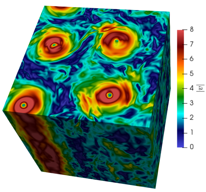
Figure 3: Right: 3d rendering of the velocity amplitude $|\bm{v}|$, in a rotating turbulent flow. Left: 3d averaged energy spectrum, $E(k)=\sum_{{\bf k}=k}^{k+1}\langle|\hat{\bm{v}}({\bf k})|^{2}\rangle$, where with $\hat{\bm{v}}({\bf k})$ we denote the Fourier coefficient at wavenumber $\bm{k}$. The forcing and the Kolmogorov wavenumbers, $k_{f},k_{\eta}$ are indicated with arrows, notice the presence of power-law energy fluctuations on almost two decades and for wavenumbers smaller and larger than $k_{f}$, the indication of the split-energy cascade scenario. Inset: standardized probability distribution function of the vorticity in the direction of the rotation axis, $\omega_{3}$. Notice the presence of strong non-Gaussian, intermittent and skewed fluctuations up to $O(10)$ (and higher) standard deviations, $\sigma$.

III Context Encoder for Image Generation (CE1)

Let us first present the context encoder as suggested in pathak2016context with reference to Figs. 2 and 4 and to appendix A for specific details. The idea is to have a Deep-GAN that reconstructs the missing part of the three velocity configurations. To that end we define the masking operator $\hat{M}$, which takes the value $1$ on the missing pixels and $0$ on the unaltered locations in our original image ${\cal I}_{v}$. We will then denote with $\hat{M}\odot{\cal I}_{v}$ the damaged part of ${\cal I}_{v}$ and with $(1-\hat{M})\odot{\cal I}_{v}$ the region of the flow where we have the full information, see Fig. 2 for a graphical representation applied to a set of three velocity components, ${\cal I}_{v}=(v_{1},v_{2},v_{3})$. The overall architecture is based on a pipeline with first the generator (G) made of an encoder which takes as input the damaged image, $(1-\hat{M})\odot{\cal I}_{v}$, produces a latent representation of the relevant features with a down-sampling of the dataset, then in the second part of the network a decoder learns how to generalise the features and proposing a candidates for the three velocity components in the missing gap, $G[(1-\hat{M})\odot{\cal I}_{v}]$. The Generator part of the context encoder, panel (a) of Fig. 4, is trained to minimize the $L_{2}$ norm between the generated image and the ground truth inside the hole:

$$\mathcal{L}_{rec}=\mathbb{E}_{{{\cal I}_{v}}}\{||\hat{M}\odot{\cal I}_{v}-G[(1-\hat{M})\odot{\cal I}_{v}]||_{2}\},$$ (2)

where $G[\bullet]$ indicates the snapshots of three velocity components provided by the network as output and with $\mathbb{E}_{{{\cal I}_{v}}}$ we intend average over the set of training configurations. The final network is supplemented with an adversarial structure, see panel (b) of Fig. 4, made of a discriminator (D) to provide loss gradients to the context generative encoder G. The learning protocol is a two-player game where the discriminator D is inputted alternatively with ground truth images in the hole or the ones generated by the context encoder G and tries to distinguish among them while the generator G tries to confuse D by proposing samples that appear as close as possible to real turbulent configuration in the missing region. The adversarial task for the discriminator component of the encoder is to maximize the binary cross-entropy function:

$$\mathcal{L}_{adv}=\mathbb{E}_{{{\cal I}_{v}}}\{\log(D[\hat{M}\odot{\cal I}_{v}])+\log(1-D[G[(1-\hat{M})\odot{\cal I}_{v}])\}$$ (3)

where $D[\bullet]$ is the output of the discriminator with values $\in(0,1)$. The above expression is maximized when the discriminator is able to assign $1$ to the real images and $0$ to the ones proposed by $G$. We notice that in the second term of the above expression we only use data proposed by the generator G in the gap of size $\ell\times\ell$ and do not supply the whole image of size $L\times L$ to not help the discriminator to exploit potential discontinuities when passing from the hole filling to the external frame.
Finally, the total loss that must be minimized to train the Generator part of the CE1 is given by a linear superposition of the two components:

$$\mathcal{L}=\lambda_{rec}\mathcal{L}_{rec}+\lambda_{adv}\mathcal{L}_{adv},$$ (4)

with $\lambda_{rec}+\lambda_{adv}=1$, and where the adversarial loss is here evaluated only with the images produced by the Generator: $\log(1-D[G[(1-\hat{M})\odot{\cal I}_{v}]).$ In the following section we will present the results by varying the typical length scale, $\ell$ of the spatial hole where data are missing but keeping the overall damaged area the same (see section III.1) or by varying the structure of the input data, using a multi-channel information made of three images of the three velocity components, $v_{1},v_{2},v_{3}$ or a single channel given by the vertical vorticity $\omega_{3}$ (see section III.2).

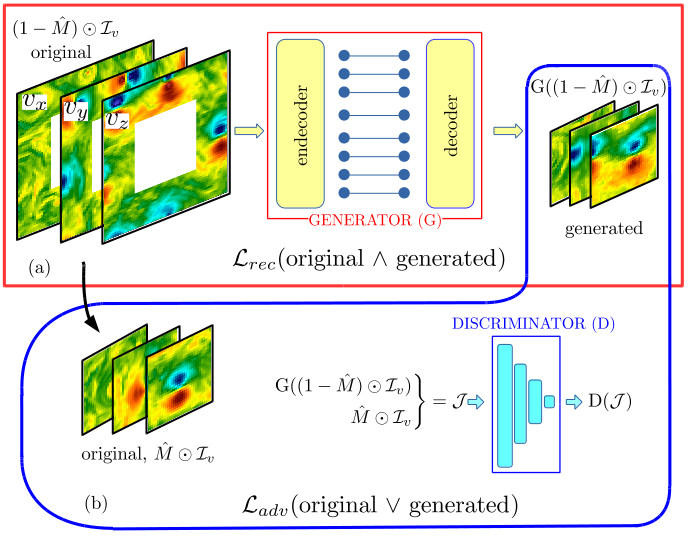
Figure 4: Sketch of the Context Encoder (CE1) configuration. The machine is made of two blocks. A Generator (G), depicted in panel (a), where we give in input the three channels made of the three corrupted configurations of size $L\times L$ with $L=64$ for the three velocity components in the plane, $v_{1}(x_{1},x_{2}),v_{2}(x_{1},x_{2}),v_{3}(x_{1},x_{2})$ and obtain as output the fields proposed to fill the gap of size $\ell\times\ell$. The second block is given by a Discriminator (D), see panel (b), which is trained to distinguish the original fields from the ones proposed by the generator for the hole region. See appendices A and B for details about the internal structure of G and D.

III.1 Image inpainting: large vs small scales information

We start by analysing the training performance and the final validation for the CE1 network by removing from the input a squared hole of size $\ell\times\ell$ with $\ell=L/2$ located at the centre of the image. Here we present data when we used in input three channels with the three velocity components in the plane and we later compare with the case when the total missing area is the same but each single missing spot is smaller.
In Fig. 5 we show the evolution of the reconstruction loss $\mathcal{L}_{rec}$, of the adversarial loss $\mathcal{L}_{adv}$ and of their weighted sum (4) obtained with $\lambda_{adv}=0.001$, measured on the validation dataset, as a function of the epochs during training, for details see appendix A. For training we have used a total number of configurations $N_{tra}=81920$ while for validation we used a set of $N_{val}=20480$ configurations never seen during training. As one can see from Fig. 5, the training converges rapidly without any over-fitting. Indeed, to improve the network generalization we have added a dropout of $20\%$ on the ‘features vector’ in CE1, see appendix A. The key idea behind dropout, is to randomly remove units (along with their connections) from the neural network during training. This prevents units from adapting too much to the training dataset and it reduces significantly over-fitting srivastava2014dropout .

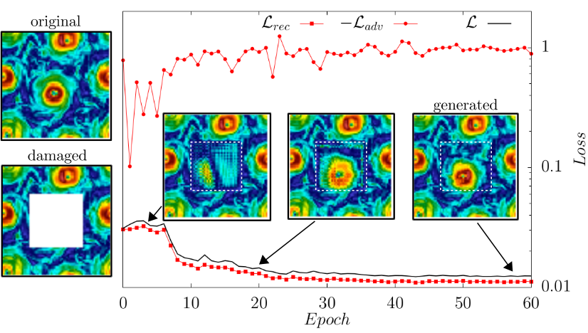
Figure 5: Example of a training section for CE1. We show the evolution of $\mathcal{L}$, $\mathcal{L}_{rec}$ and $-\mathcal{L}_{adv}$, measured on the validation dataset, as a function of the epoch as well as the reconstructed configuration for $|\bm{v}|$ at three different steps during training. Notice the tendency to supply better and better inpainting by advancing the learning protocol. The two pictures on the left represent the ground truth in the whole plane and the damaged input.

In the inset of the same Fig. 5 we show the quality of the gap filling at different epochs, to give a visual demonstration of the ability of CE1 to progressively learn the correct flow structures. Each mini-batch used in our training is composed of $128$ images and each epoch consists of $640$ mini-batches (see appendix A for more details). Training has been performed also with a smaller number of mini-batches but obtaining worse results. Hyper-fine optimization in the size of each mini-batch has not been performed because not our main interest here.

We now proceed with a more quantitative analysis of the CE1 performances using the network frozen at its final epoch configuration. In Fig. 6 we show a series of 3 different gap filling experiments using configuration never showed during training as well as a point-wise analysis of the normalized $L_{2}$ norm calculated on vertical lines for each fixed horizontal position, $x_{1}$:

$$\Delta_{v}(x_{1})=\frac{{\ell^{-1}\sum_{x_{2}}\sum_{i=1}^{3}[v^{truth}_{i}(x_{1},x_{2})-G_{i}(x_{1},x_{2})]^{2}}}{E_{tot}}$$ (5)

where $G_{i}(x_{1},x_{2})$ for $i=1,2,3$ are the three components of the field generated by CE1 inside the missing region. The above expression is normalized dividing by the averaged flow energy over a subset of $N=2048$ of the validation dataset that are the configurations used in our reconstruction experiment: $E_{tot}={L^{-2}\sum_{x_{1},x_{2}}\sum_{i=1}^{3}\langle[v^{truth}_{i}(x_{1},x_{2})]^{2}}\rangle_{N}$, where we used $\langle\bullet\rangle_{N}$ for a shorthand notation of the average.

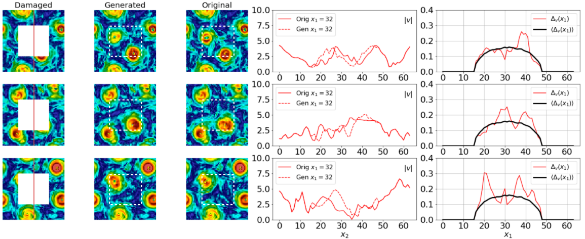
Figure 6: Validation of gap filling by CE1 for three different generated fields (one for each row). Images show the magnitude of local velocity field, $|\bm{v}(\bm{x})|$. 1st column: damaged image in input. 2nd column: image generated in output. 3rd column: ground truth. 4th column: generated (dashed) and ground truth (solid) profiles of $|\bm{v}(\bm{x})|$ along the vertical line shown in the 1st column. 5th column: $L_{2}$ error, $\Delta_{v}(x_{1})$ vs $x_{1}$, given by expression (5) for each image (red line) and the average error $\langle\Delta_{v}(x_{1})\rangle_{N}$ over $N=2048$ different images (black curve).

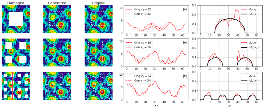
Figure 7: The same as in Fig.(6) at changing the typical size of the damaged region, $\ell/L=1/2,1/4,1/8$ from top to bottom rows.

It is interesting to notice (5th column, red line) that the local normalized $L_{2}$ error for each snapshot is of the order of $10-20\%$, when we are in the middle of the missing region, showing a very good reconstruction property of our CE. In the same panels we plot the averaged errors, $\langle\Delta_{v}(x_{1})\rangle_{N}$. As on can see, the max averaged error is $O(15)\%$ (black lines). Notice also that the error slightly improve for horizontal position close to the gap edge, indicating that the network is able to detect local correlations also. In Fig. 7 we test the CE1 at changing the spatial distribution of the missing data, by distributing the same amount of total gaps but on squares with smaller and smaller size $\ell/L=1/2,1/4,1/8$. As one can see from the black curves in the last column of the same figure, the averaged errors, $\langle\Delta_{v}(x_{1})\rangle_{N}$, become smaller and smaller by decreasing $\ell$, reaching a maximum averaged error as small as $3-4\%$ for $\ell/L=1/8$. It is important to stress that this is a very good result, being the corrupted size still much bigger than the differentiable limit given by the Kolmogorov scale $\eta=1/k_{\eta}\sim\ell/L=1/64$, (see Fig. 3). In other words, we always work in the scale range where the fields are rough and non-differentiable with Holder continuity close to $1/3$ frisch1995turbulence , making the problem much different from the one of non-linear local fit that other classical inpainting methods can handle well bertalmio2000image ; barnes2009patchmatch ; efros1999texture ; osher2005iterative . In the rightmost panel of Fig. 8 we show the most stringent test one can perform, checking the point-by-point reconstruction properties by plotting the probability distribution function of the local $L_{2}$ error:

$$\Delta_{v}(x_{1},x_{2})=\frac{{\sum_{i=1}^{3}[v^{truth}_{i}(x_{1},x_{2})-G^{v}_{i}(x_{1},x_{2})]^{2}}}{E_{tot}}.$$

The panel shows that we obtain a pretty good performance to assimilate data even local-wise with very small probability to make big errors. Furthermore, when $\ell/L$ becomes small there is a sharp improvement for the worst case as shown by the sharp reduction in the right tail extension when comparing $\ell/L=1/8$ with $1/2$.

In Fig. 8 we perform also two less stringent statistical test concerning the reconstructed flow. First, in the left panel we show the 2d spectrum:

$$E(k)=\sum_{k<{\bm{k}}<k+1}\langle\hat{v}_{i}({\bm{k}})\hat{v}_{i}({-\bm{k}})\rangle_{N}$$ (6)

where ${\bf k}=(k_{1},k_{2})$ and we calculated the Fourier transform of the velocity field, $\hat{v}_{i}({\bf k})$, over the whole 2d configuration with the gap filled as proposed by the output of CE1. In the same panel we also show the spectrum calculated on the corrupted input to quantify how much information (energy) we miss at different scales. Curves here are averaged over $N=2048$ configurations. In the same figure, middle panel, we show the probability distribution functions (PDF) for the velocity magnitude, $v$, and for the out-of-plane vorticity, $\omega_{3}$. All comparisons between generated and the ground truth are very good even for the strongly non-Gaussian distribution enjoyed by the $\omega_{3}$ field.
In Fig. 9, we focus on the comparison of purely turbulent quantities, namely, the energy transfer across scales $\Pi_{\Delta}$ and the structure functions $S_{p}(r)$ up to $p=4$. To define the energy transfer in physical space we follow the approach common in large-eddy-simulations (LES) Pope00 ; meneveauARFM ,

$$\Pi_{\Delta}=\partial_{j}\bar{v}_{i}\left(\overline{v_{i}v_{j}}-\overline{\bar{v}_{i}\bar{v}_{j}}\right)\ ,$$ (7)

where the $i,j$ indices run over the two velocity components parallel to the plane, namely $(1,2)$. Both coarse-grained velocity components, ${\bar{v}_{i}}$, are obtained by a convolution operation between the velocity field $v_{i}(\bm{x},t)$ and a filter kernel $G_{\Delta}(\bm{x})$,

$${\bar{v}_{i}}(\bm{x},t)\equiv\int_{S}d\bm{y}\ G_{\Delta}(|\bm{x}-\bm{y}|)\ v_{i}(\bm{y},t),$$ (8)

where $S$ represents the plane surface. In particular, as filter kernel we have used the ‘sharp spectral cutoff’ in Fourier space Pope00 with a cutoff $\Delta=\pi/k_{c}$ and $k_{c}=16$. The main panel of Fig. 9(a) shows the PDF of $\Pi_{\Delta}$ constrained on the damaged area of the velocity planes, from which we can see the good agreement between original and generated data both showing the same deviation from gaussianity. In the inset of the same figure two visualizations of the energy transfer on the same plane either from the original or the reconstructed fields are presented to appreciate visually the good quality reached in the reconstruction by CE1 network. In panel (b) of Fig. 9, in order to estimate the quality of the reconstruction in terms of velocity correlations at different scales, we analyse the statistics of the longitudinal velocity increments defined as $\delta_{r}v=(\bm{v}(\bm{x}+\bm{r})-\bm{v}(\bm{x}))\cdot\bm{r}/r$ frisch1995turbulence . In particular in Fig. 9(b) we compare the 3rd and the 4th order structure functions, defined as;

$$S_{p}(r)\equiv\langle[\delta_{r}v]^{p}\rangle,$$ (9)

where the $\langle\cdot\rangle$ means an average over the planes and all the $2048$ reconstructed fields. Also from this analysis we found a high agreement between original and reconstructed data. In the main panel we present the log-log plot of $S_{4}(r)$ data, from which we can see a perfect collapse between the original and generated data. In the inset of the same figure the third order structure function is presented in log-lin scale from which we can appreciate that also the change in the sign of $S_{3}(r)$ is captured by the CE1 reconstruction.

As a final statistical analysis of the reconstructed images we show, in Fig. 10, a scatter plot of the extreme values of the velocity (in panel (a)) and vorticity (in panel (b)) coming from the original data and the field generated by CE1 inside the predicted region. There is a very good correlation between the original and reconstructed data for both quantities, indicating that the CE1 is able to properly reproduce the correct maximum value inside each gappy region.

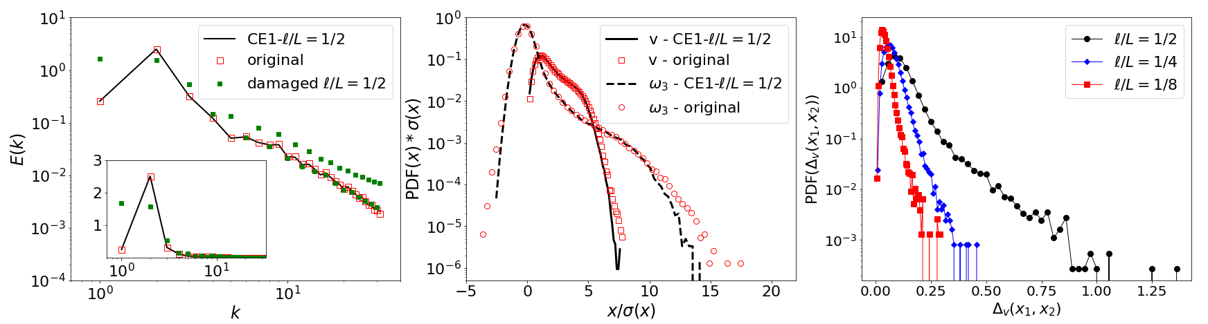
Figure 8: Left: comparison between the 2d spectrum (6) of the ground truth original DNS data in the whole 2d plane and the data reconstructed by the CE1 with $\ell/L=1/2$, as well as the spectrum calculated on the damaged image; the inset shows the same data in log-lin scale. Middle: comparison of standardised PDFs of velocity magnitude, $v=|\bm{v}|$ and vorticity $\omega_{3}$. Right: Lin-Log PDF for the point-wise $L_{2}$ error, $\Delta_{v}(x_{1},x_{2})$ at changing $\ell/L$.

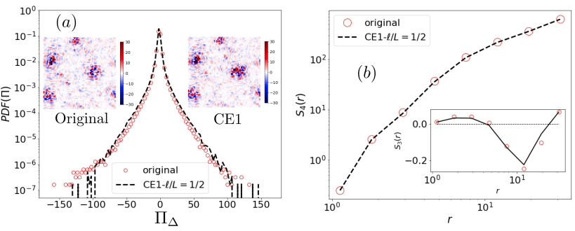
Figure 9: Panel (a): Comparison of the PDF of the energy transfer $\Pi$ measured inside the damaged region from both the original (red circles) and reconstructed data using CE1 network (dashed black line). Panel (b): Comparison of the longitudinal structure function, $S_{p}(r)$, for both original (red circles) and reconstructed data (dashed black lines). In the main panel $S_{4}(r)$ is presented in log-log scales, while in the inset the 3rd order structure functions, $S_{3}(r)$ are presented in log-lin scale.

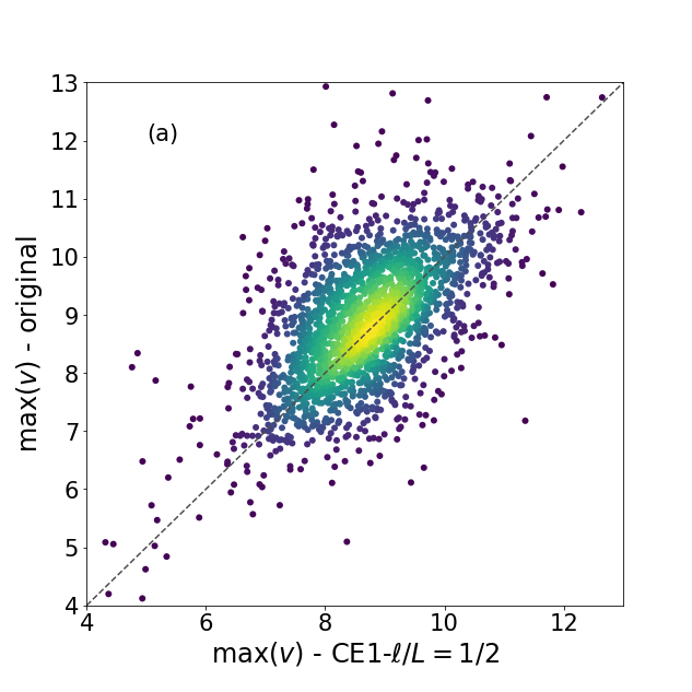
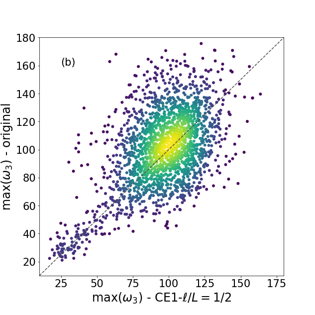
Figure 10: Scatter plot of the maximum values inside the reconstructed region of the (a) velocity and (b) vorticity calculated from the original data and the one produced by CE1. Colours are proportional to the density of points in the scatter plot.

III.2 Features ranking

In this section we discuss a different question, connected to use DA tools as a reverse engineering approach to perform features ranking, i.e. to assess the quality and quantity of the input data on the basis of the obtained output. To do that, one can change the set of fields supplied in the CE input and/or change the definition of the loss function in order to optimize some features of the generated output. Let us suppose, for example, that we want to reconstruct with high accuracy only the out-of-plane vorticity field, $\omega_{3}$. One question one can ask is that weather it is better to work with (i) the three velocity channels as input and optimising the reconstruction against the corresponding three velocity outputs in the missing gap, as done in the previous section, (ii) $w_{3}$ as input and output (one channel only) or (iii) using $v_{1},v_{2},v_{3}$ as input but adding in the loss also a penalization against bad reconstruction of gradients. The idea is to test the importance of having both large and small-scales information in the CE1 input/output, i.e. semantic contents that have larger and smaller influence size. The two above cases labelled with (ii) and (iii) would correspond to the following loss function:

$$\mathcal{L}_{rec}=\mathbb{E}_{{{\cal I}_{\omega}}}||\hat{M}\odot({\cal I}_{\omega}-G[(1-\hat{M})\odot{\cal I}_{\omega}])||_{2}$$ (10)

for case (ii) and to

$$\mathcal{L}_{rec}=\alpha\mathbb{E}_{{{\cal I}_{v}}}\{||\hat{M}\odot({\cal I}_{v}-G[(1-\hat{M})\odot{\cal I}_{v}])||_{2}\}+(1-\alpha)\mathbb{E}_{{{\cal I}_{v}}}\{||\hat{M}\odot(\omega_{3}\odot{\cal I}_{v}-\omega_{3}\odot G[(1-\hat{M})\odot{\cal I}_{v}])||_{2}\}$$ (11)

for case (iii), where with $\omega_{3}\odot$ we intend the operation to extract the $\omega_{3}$ component out of the three $v_{1},v_{2},v_{3}$ original fields, ${\cal I}_{v}$ or of the ones generated by $G[\bullet]$ and we have introduced a parameter $\alpha\in[0:1]$ that weighs the loss due to reconstruction of $\bm{v}$ and the one due to $\omega_{3}$. In the first row of Fig. (11) we show the results for vorticity reconstruction for case (i), with loss given by Eq. (3), while in second and third rows we show the same but for cases (ii) and (iii), which correspond to losses given by Eqs. (10) and (11), respectively. The latter obtained with mixing parameter $\alpha=0.5$. Comparing results from first and second row, $\langle\Delta_{\omega_{3}}(x_{1})\rangle\sim 55\%$ and $75\%$ respectively, we see that in order to have an improved reconstruction of vorticity it is better to train with the whole set of three velocity field (first row, case i) than using vorticity directly (second row, case ii). This is somehow natural because for the former we have more information in input than in the latter. Moreover, vorticity is a highly skewed and non-Gaussian variable frisch1995turbulence , properties that could be problematic to handle as input in the network as done in case (ii). Conversely, by comparing first and third rows, cases (i) and (iii), we learn that keeping the three velocity in inputs (max information) and penalising the output in terms of the $L_{2}$ norm for vorticity does help to give a better reconstruction decreasing $\langle\Delta_{\omega_{3}}(x_{1})\rangle$. Let us notice, however, that the final result is never exceptionally satisfying, with averaged errors in the middle of the missing region that are always around $35\%-40\%$, at the best. From the right panel of Fig. 12 we can indeed see that even for the better results, case (iii), the PDF of the point-wise reconstruction error has now a pretty extended right tail, indicating the partial failure to have a good local reconstruction, even though the spectral and PDF for the vorticity field are satisfactorily reproduced (left and middle panel). The difficulty to reconstruct point-wise the correct vorticity properties can be due to different reasons. First, the field is strongly non-Gaussian and with a very small spatial correlation length of the order of $\eta$, hence much smaller than $\ell$. Second, as one can see from the first three columns of Fig.  11 it is enough a small mismatch for the position of the vorticity peaks between the ground truth and the reconstructed images to produce a big local error while the overall image is still very close to the original one. Third, vorticity field is obviously much more sensitive to small details, with a Fourier spectrum enhanced by a factor $\propto k^{2}$ wrt the kinetic energy case, something that is particularly critical in the presence of rough non-differentiable fluctuations as in our turbulent case.

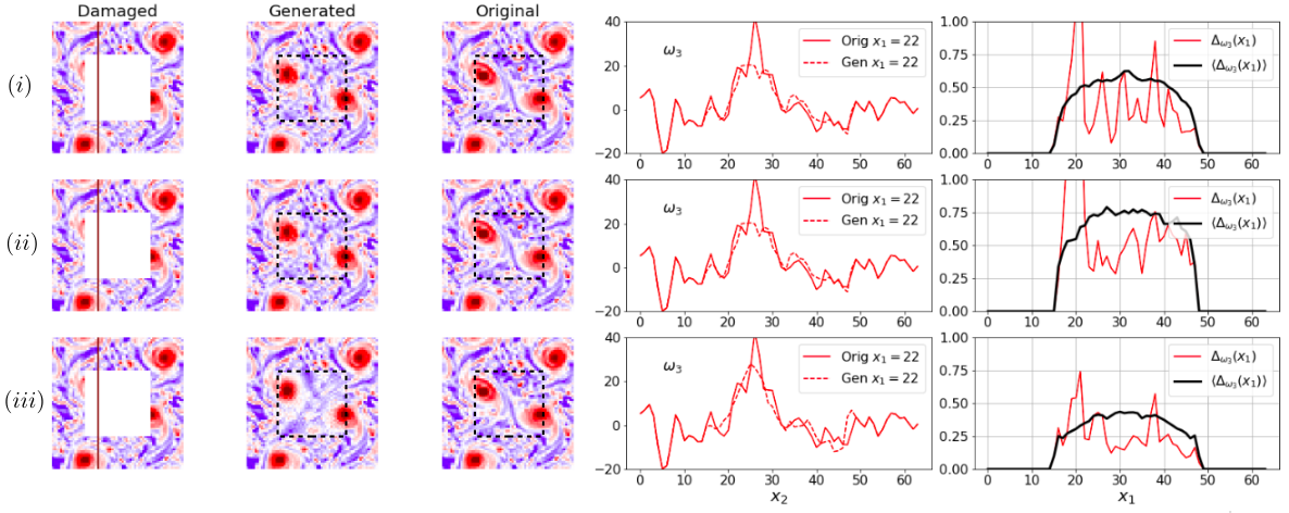
Figure 11: Vorticity reconstruction with CE1. Comparison for vorticity generation using loss given by case (i), Eq. (4) first row; obtained by using vorticity in input and in output as in case (ii), Eq. (10), second row; and for case (iii), Eq. (11) third row. Errors are defined following Eq. (5)

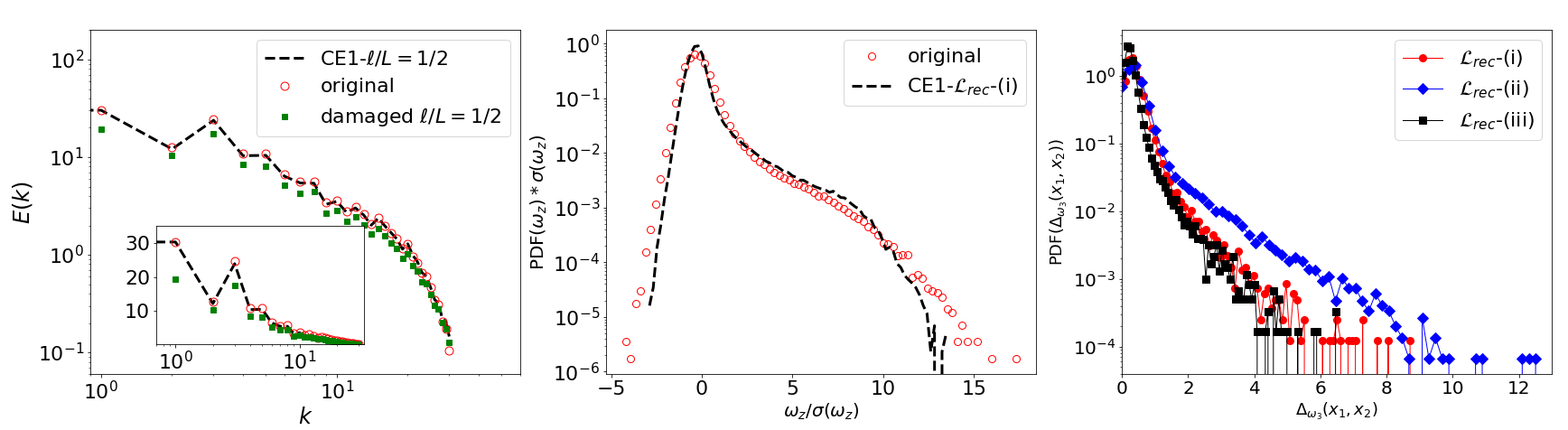
Figure 12: Left: comparison between spectrum of vorticity for ground truth (original DNS data in the whole 2d plane), for the data reconstructed by the CE1 with $\ell/L=1/2$ using the protocol based on the loss function of case (iii) given by Eq. (10) and for the spectrum calculated on the damaged input images, inset the same but in log-lin scale. Middle: comparison for standardised PDFs of vorticity $\omega_{3}$. Right: Lin-log plot of the PDF for the point-wise $L_{2}$ error, $\Delta_{v}(x_{1},x_{2})$ using the three different CEs trained with the loss functions for cases (i-iii).

IV Context Encoder with back-propagation to the input data (CE2)

The second context encoder we analyze is based on the concept of constrained image generation yeh2017semantic . The idea proceeds in two steps. First a GAN is trained to generate uncorrupted flow configurations in the whole 2d domain, see Fig. 13. The generation is conditioned on a set of random input values, ${\bf z}=(z_{1},z_{2},\dots,z_{T})$, with $T=100$ in our case, which are transformed by the trained machine in realistic flow configurations, at least as realistic as being not distinguishable from the discriminator in the GAN itself.

Figure 13: Sketch of the Context Encoder (CE2) configuration. The machine is made of a typical Deep-GAN structure yeh2017semantic ; goodfellow2014generative which is pre-trained to generate output images on the whole 2d plane, $G[{\bf z}]$ from a random input ${\bf z}$. To apply it for gap-filling, the GAN is frozen and a back-propagation to the input data is implemented. Only ${\bf z}$ is evolved to match the given corrupted image, $(1-\hat{M})\odot{\cal I}_{v}$, where we have data.

Then, the GAN is frozen and for the image reconstruction task a search for the optimal set of ${\bf z}$ inputs is performed, asking the machine to reproduce with high fidelity only the uncorrupted region. The idea is that once the GAN is trained to generate the entire turbulent snapshots, we just need to search for the closest configuration that can be generated by the machine and that matches the known data, $(1-\hat{M})\odot{\cal I}_{v}$. Moreover, also a penalty against generation of patches that are disconnected by the frame will be added, via the insertion of a discriminator loss (see below and Fig. 13). At difference form CE1, here we do not use the structure of the mask for training. After the Deep-GAN has been trained goodfellow2014generative ; denton2015deep ; simonyan2013deep we proceed to recover the optimal ${\bf z}^{*}$-encoding that is closest to the corrupted image. After ${\bf z}^{*}$ is obtained we can input it to the GAN to obtain the whole configuration also inside the gaps. In practice, in order to fill one damaged field, $(1-\hat{M})\odot{\cal I}_{v}$, we obtain ${\bf z}^{*}$ by minimizing the combined loss:

$$\mathcal{L}=\mathcal{L}_{rec}+\lambda_{adv}\mathcal{L}_{adv}$$ (12)

where

$$\mathcal{L}_{rec}=||{(1-\hat{M})}\odot({\cal I}_{v}-G[{\bf z}])||_{2}$$ (13)

by back propagating with respect to the input data: $-\partial_{{\bf z}}\mathcal{L}_{rec}$, where we need to notice that in (13) we are using information only on the available data by applying the mask $(1-\hat{M})$ to all velocity components. The second term in (12) is giving a penalty if the generated image on the whole domain does not look similar to a real turbulent configuration, by applying the judgement of the (previously trained) discriminator D:

$$\mathcal{L}_{adv}=\log(1-D[G[{\bf z}]])$$ (14)

where $\lambda_{adv}=0.1$ is a parameter used to balance between the two losses and where the input data are updated to fool D, $-\partial_{{\bf z}}\mathcal{L}_{adv}$. In Fig. 14 we show the equivalent of Fig. 7 for three different experiments using CE2. As one can see from data in column 5, now there is a non zero error, $\Delta_{v}(x_{1})$ also outside the missing region because CE2 generate the flow in the whole domain. The overall performances have a maximal averaged error $\langle\Delta_{v}(x_{1})\rangle$ of the order of $40\%$ roughly a factor 2 larger than CE1. It is important to stress again that we didn’t perform any systematic optimization of network structures and/or learning parameters being primarily interested here to the proof of concept aspects. In Fig. 15 we show the comparisons against the DNS (ground truth) for spectra, velocity and vorticity PDFs, again with good overall results but worse performance with respect to CE1, especially concerning the PDF of the local $L_{2}$ norm (right panel), which presents now a fatter right tail.

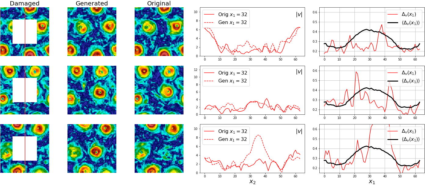
Figure 14: The same of Fig. 6 but for CE2. Notice the 3rd row, where the network puts a vortex in the gap region which is not present in the original case, hence the big error $\Delta_{v}(x_{1})$ for $x_{1}\sim 40$.

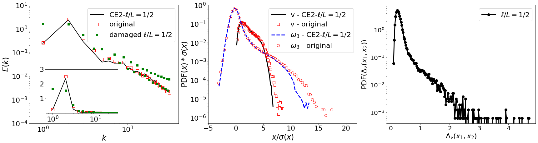
Figure 15: The same as in Fig. 8 but for CE2. Comparison for spectra (left), PDF of velocity and vorticity (middle). Right: Lin-log plot of the PDF for the point-wise $L_{2}$ error calculated in the whole area.

V Equation-informed DA: Nudging

In this section we confront the results obtained with CE1 and CE2 against what one can achieve using Nudging Hoke76 ; Lakshmivarahan13 ; clark_di_leoni_synchronization_2020 , a DA scheme popular among numerical weather forecast community and in economic fields benartzi2017should . Nudging is distinguished from the methods presented above in two senses: it relies entirely on solving the equations of motion and it is also applicable to reconstruct trajectories in phase space. The scheme works by introducing a relaxation term to the equations of motion, penalizing the flow when it deviates from a given reference state, set by the data one wants to reconstruct/assimilate. In rotating turbulence it takes the following form:

$$\frac{\partial\bm{v}}{\partial t}+\bm{v}\cdot\bm{\nabla}\bm{v}+2\Omega\hat{x}_{3}\times\bm{v}=-\bm{\nabla}p+\nu\nabla^{2}\bm{v}+\gamma(1-\hat{M})_{x_{3}}\odot(\bm{v}-\bm{v}_{\rm ref})$$ (15)

where $\gamma=100$ is the intensity of the nudging, $(1-\hat{M})_{x_{3}}\odot$ is the same filtering operator used in the previous section, replicated identically along the $x_{3}$ direction, such that the nudging term acts only on the locations where the reference damaged flow, $\bm{v}_{\rm ref}$, is known. The idea behind the method is simple, instead of using a machine to learn (local and non-local) information in the 2d images we ask the NSE to provide the semantic background to fill the gaps, providing the whole 3d field in the whole volume $\bm{v}(\bm{x},t)$ and for all times. Notice that NSE need to be evolved on the original volume size, even if the input is masked to be a subset of a 2d slice. Notice also that usually Nudging is used to reproduce also temporal evolution, while here we will implement it to reconstruct one given, frozen in time, 2d velocity snapshot (which is replicated identically along the $x_{3}$). Another important difference wrt Context Encoders is that we do not need any training section using hundred thousands examples from the ground truth as in ML applications, provided that the equations used are the ones that have also generated the corrupted images. It is also key to realize that we do not need to supply any external mechanical forcing mechanism to (15), i.e. the reconstruction is obtained without knowing the external stirring. Nudging was shown to be able to reconstruct, with different degrees of accuracy, high Reynolds number three dimensional turbulent flows clark_di_leoni_synchronization_2020 , two dimensional flow Gesho16 ; Farhat16 and Rayleigh-Bernard convection Farhat19 . Moreover, Nudging can make up for inferring missing terms in the equation, such as forcing or even rotation Clark18 . In the following we show the performance of nudging to reconstruct missing hole in the middle of a 2d slice exactly as we did before for the two Context Encoders. We performed a long numerical integration of (15) on the original box size, with $256^{3}$ collocation points and supplying the 2d damaged input given by $(1-\hat{M})_{x_{3}}\odot{\cal I}_{v}$, where ${\cal I}_{v}$, denoted here $\bm{v}_{ref}$ to follow the notation used by the community, is the three velocity components in a $64^{2}$ 2d plane $(x_{1},x_{2})$. As said, the image is extended along the vertical direction in order to form a 3d volume (but no vertical fluctuations are introduced as we just stack up the same image). The resulting reference field for the nudging algorithm is constant in time. In this way we are not providing any extra information (vertical or temporal fluctuations) compared with the CE1 and CE2 cases discussed above. With this in mind, the result coming from the nudging is obtained as an average both in time and along the vertical direction.

In Fig. 16 we show the results of one of our experiments at changing $\ell/L$ following what done for the CE1 and shown in Fig. 7. As for CE2 case, nudging is introducing errors also where data are supplied, because NSE evolves in the whole (3+1)d domain. From the data shown in column 5, we can see that the averaged error $\langle\Delta_{v}(x_{1})\rangle$ is more noisy wrt to the CE1 and CE2 corresponding cases. This is due to the fact that we performed only three experiments with different nudging fields because of the much heavier computational overhead introduced by the need to solve NSE for each test. Nevertheless, we notice that the overall errors are of similar order wrt to Figs. 7-14, although some small-scale reconstruction deficiencies can be spotted for the bigger gap case $\ell/L=1/2$ (first row). Some of these problems could be mitigated if the reference field is not constant in time clark_di_leoni_synchronization_2020 .

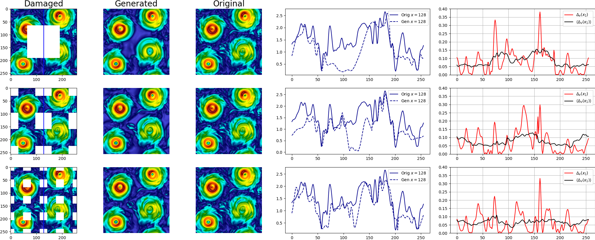
Figure 16: The same as in Fig.(7) but for nudging. Here in the 2nd column we show the average in time and along the $x_{3}$ direction of the nudged-NSE (15) output, $\langle|\bm{v}(x_{1},x_{2})|^{2}\rangle_{t,x_{3}}$. In the 5th column, the black curve is obtained with a further average over three different nudging experiment.

VI Conclusions

We have presented a series of investigations meant to test the applicability of tools widely used by the CV community for image inpainting to turbulent data reconstruction from the TURB-Rot database turbrot . At difference from the typical set of images database where CV algorithms are trained, our case is made of a series of complex scenes, with random properties and multi-scale fluctuations. We have presented results for two different Context Encoders, called CE1 and CE2. CE1 is able to provide (once trained) a guess for the missing data without any further inference. Contrary, CE2 is based on a two step training, first the machine learns how to generate ungappy images and second it specialises to further fill the gap, needing a new training phase for each new filling. Results among the two are very satisfactory with CE1 performing better, even though a few caveats must be made. First, we didn’t try to push the hyper-parameters settings to a level that cannot be improved further. Second, we do not think there exists ‘the best’ method to reconstruct and assimilate turbulent data. Turbulence has many common features but also many small subtle differences in different realization in nature and in the labs. So, the question ‘what is the best method to assimilate turbulent data’ is not well posed. Even for the same set-up, different methods can have different level of optimality depending on the quality and quantity of missing data, a trivial example being given by the case when data are missing in regions of size smaller than the Kolmogorov scale, where any nontrivial interpolation scheme would reconstruct pretty well. Similarly, all ML tools need to be retrained in the presence of big changes in the context: robustness and generalization being very limited. The scope of this paper is to present two different ML tools, and show that we have new tools in the box. Optimality and uniqueness of reconstruction cannot be proven rigorously due to the high dimensionality of the phase-space and the presence of rough (multifractal) flow configuration. To this end we provide the whole database online and open such as to trigger the interested community to improve our results turbrot . We found that the two CE algorithms are good also for semantic filling, i.e. when a big part of the image is missing, with maximum average L2 error of the order of $10\%$ that must be considered good or bad depending on the other methods that one can apply. In our case, we do not know of any other attempt to try to reconstruct such a kind of complex flow as we did here and we consider the result highly non trivial. We found that large-scale features (velocity components) are reconstructed better than small-scale ones (vorticity) and that for the latter it is key to provide the whole set of velocity components in input to improve the inpainting. Point-to-point reconstruction in turbulence is theoretically limited by the presence of spatio-temporal chaos, which makes the configuration in any region (or time window) strongly sensitive to the boundary (or initial) conditions. As a result, it is not surprising that the vorticity field is less accurately reconstructed, given the very short correlation length of turbulent gradients. Statistical reconstruction is easier, and indeed our two CEs are performing well for this aspects, as shown by the middle panels of Figs. 8, 12, 15 and in Figs. 9 and 10. It would be interesting to apply the same techniques to flows with a mean profile, to see if the presence of non-statistical information is helpful to condition also the fluctuating fields.

Finally, we present results using Nudging, an equation-informed tool well established among the applied communities in numerical weather forecasts, geophysics and others. For our application, Nudging requires a new simulation of a 3d fully developed turbulent flows for each data reconstruction experiment and thus it is computationally much heavier than the two ML algorithms (if already trained). The trade-off is that Nudging will provide for a field reconstruction that is fully respectful of all symmetries and kinematic constraints enjoyed by the PDE, something that is not always easy to achieve with Convolutional Neural Networks. For instance, CE2 was trained without imposing periodic boundary conditions on the whole domain, a feature that the GAN needed to discover by itself. It will be interesting to study the trade-off between simplicity of the implemented GAN architecture and the accuracy obtained by imposing known physical constraints raissi2019physics ; wu2020enforcing ; wang2019towards ; erichson2019physics ; lusch2018deep ; kashinath2020enforcing ; mohan2020embedding

Another advantage of Nudging is that it does not need training, it works even with one damaged configuration only, it relies on the temporal evolution of the NSE to explore the phase space and provide a realistic prior for the missing information (see pawar2020long for a recent attempt to fuse nudging with recurrent neural network). It would be interesting to compare it with other ML tools that are also based on one single image analysis to infer the statistics of the missing region ulyanov2018deep ; de2019data . It is important to notice that the application we have selected, fully developed turbulence with rotation, presents highly non-trivial aspects, e.g. multi-scale non-differentiable fields with fluctuations over 2-3 decades, without a mean flow, or boundaries. As a result, many techniques based on texturing efros1999texture , non-linear interpolation shen2002mathematical or modal analysis scherlrobust , as well as patch methods that search similar patterns in the available image barnes2009patchmatch could be in troubles to get the same accuracy. Moreover, we reconstruct only one slice of the whole 3d domain, so without any hint on the 3d features (or on temporal evolution). In conclusions, we have provided a first attempt for flow reconstruction by using state-of-the-art context encoders based on Deep-GAN, and applying it to a paradigmatic hard problem for fluid dynamics. Many qualitative and quantitative questions remain open, e.g. what happens when the damaged area is irregular and multiscale? what about 3d reconstruction or (3+1)d when also time is entering in the measurements, or applications to PIV techniques nobach2009limitations ? For the former, there is a huge literature in the CV community regarding inpainting under different quality of damages and the tools are pretty robust and flexible. Similarly, there exists inpainting ML techniques for 3d images and videos, including temporal information also. E.g., to extend our idea to deal with 3D input configurations instead of 2D images, the initial part of the encoder in CE1 or the discriminator of CE2 network should be modeled using 3D CNNs, which are now mature enough to be computationally efficient and usable (see ji20123d ; kpkl2019resource ). Exploiting temporal correlation is also a promising direction, typically hindered by the problem of large scale sweeping effects, calling for the need to follow fluid structures and extreme events in a quasi-Lagrangian reference frame.

When applying ML tools to turbulence, we need to use quantitative benchmarks to assess the performance of different networks, being visual comparisons or the spectral properties obviously not enough for such complex physics. In particular, for DA and tools there is the need to assess with local $L_{2}$ norm the goodness of the results, being interested to reconstruct non-Gaussian fluctuations in the correct position and with the correct intensity.
We hope this study will trigger other systematic validation and application of ML algorithms to complex turbulent features.

Appendix A CE1

For the implementation of the CE1 we used TensorFlow tensorflow2015-whitepaper libraries with a Python interface, optimized to run on GPUs. As introduced in Sec. III, the overall architecture is composed by a Generator plus an adversarial Discriminator network. The Generator can be further divided into an encoder and a decoder part, see Fig.17. The encoder is asked to identify all the relevant features of the three damaged images corresponding to the three velocity components. We have an input of size $64\times 64\times 3$, where we masked with $0$ values the gap region of size $\ell\times\ell$. The encoder is based on several convolutional layers with stride $2$ that reduce the dimension of the input up to a $4\times 4$ image. The last layer of the encoder, composed of $256$ convolutional filters, is reshaped in a way to form a one-dimensional features vector of size $4096$ given in input to the decoder part of the generator. A $20\%$ dropout is added to the features vector such as to reduce over-fitting. The decoder architecture that completes the Generator part, is symmetric with respect to the encoder, and it is made of several layers of transposed convolutions such as to bring the features vector to the size of the original missing region, in our case of $32\times 32\times 3$.

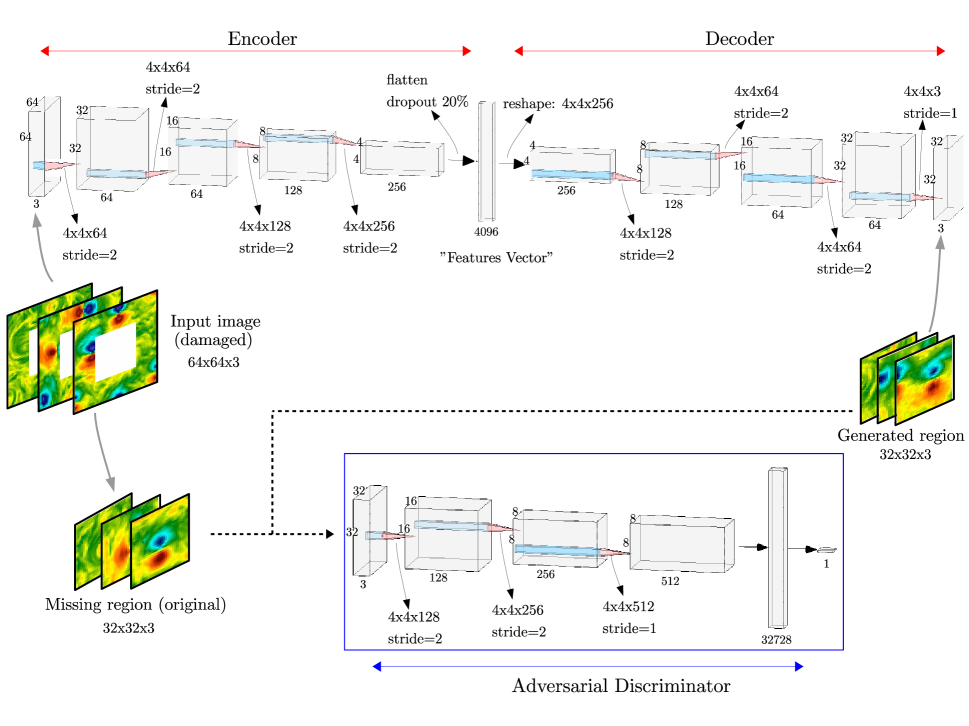
Figure 17: Sketch of the context encoder, CE1, architecture used for semantic inpainting with joint reconstruction and adversarial loss. Here and in the following figure visualization is obtained using NN-SVG software, lenail2019nn .

A first evaluation of the quality of the generated patch is measured by the $L_{2}$ norm of the difference between the generated and the original portion of the image, as we shown in eq. (2). The quality of the generated image is generally blurred and to reach a sharper reconstruction a joint loss with an adversarial architecture is required pathak2016context . The discriminator, shown at the bottom of Fig.17, is asked to recognize the original from the generated image without looking at the context but only comparing the data in the missing region and the generated part pathak2016context . The discriminator architecture similarly to the encoder is based on several convolutional layers that transform the input of size $32\times 32\times 3$ to a one-dimensional vector that is then transformed by a fully connected layer and a softmax activation function to the binary probability of the input image to be original or generated. All convolutional layers in the network are connected with LeakyRELU activation functions with a coefficient of $0.2$. The total loss defined in eq. (4) is then constructed by weighting the reconstruction and the adversarial terms with the following factors, $\lambda_{rec}=0.999$ and $\lambda_{adv}=0.001$. From the evolution of the two losses during a typical training experiment as shown in Fig. 5, we can see that $\mathcal{L}_{adv}$ is almost two orders of magnitude higher than $\mathcal{L}_{rec}$, hence from the choice of $\lambda_{adv}$ and $\lambda_{rec}$ discussed above we can conclude that the discriminator loss was found to be optimal when its weight is around $10\%$ of the total loss $\mathcal{L}$. It is important to stress that to achieve a good training with the factors discussed above, we have normalized the input data to be in the $[-1;1]$ range, namely we rescaled the intensity of each pixel by subtracting first the mean, $m=\frac{\max(\mathcal{I}_{v})+\min(\mathcal{I}_{v})}{2}$, and then normalising by $\delta=\frac{\max(\mathcal{I}_{v})-\min(\mathcal{I}_{v})}{2}$, where the maximum and the minimum are calculated over the whole training set of size $N_{tra}$. The Generator output was then shifted and rescaled back to match the original range of the velocity fields. To reach a better balance between the Generator and the Discriminator parts we used a learning rate for G $2$ times higher than that of the D. In particular the context encoder was trained with a learning rate of $2\times 10^{-4}$ while the discriminator learning rate was fixed at $1\times 10^{-4}$. The optimizer used to train the network is ADAM with parameters $\beta_{1}=0.5$, $\beta_{2}=0.999$ and $\epsilon=10^{-8}$, see kingma2014adam . The mini-batch used in our training is composed of $128$ images. Hence, because $N_{tra}=81920$, each epoch consists of $640$ mini-batches. After every mini-batch is analysed the network weights are updated back-propagating the mean error estimated on the mini-batch. For the application to case (ii) of Sec. III.2 the structure of the network is the same except that in input and output we have one image instead of three. A first validation for the reconstruction of 2d slices of a simple random 3d Taylor-Green flow is shown in Fig. 18. Being the flow differentiable and not-multiscale, the reconstruction task is achievable with a non-linear interpolation. In the figure we show that the network CE1 is able to fulfill the requirement within 1 part over 1 thousand even for the largest gap.

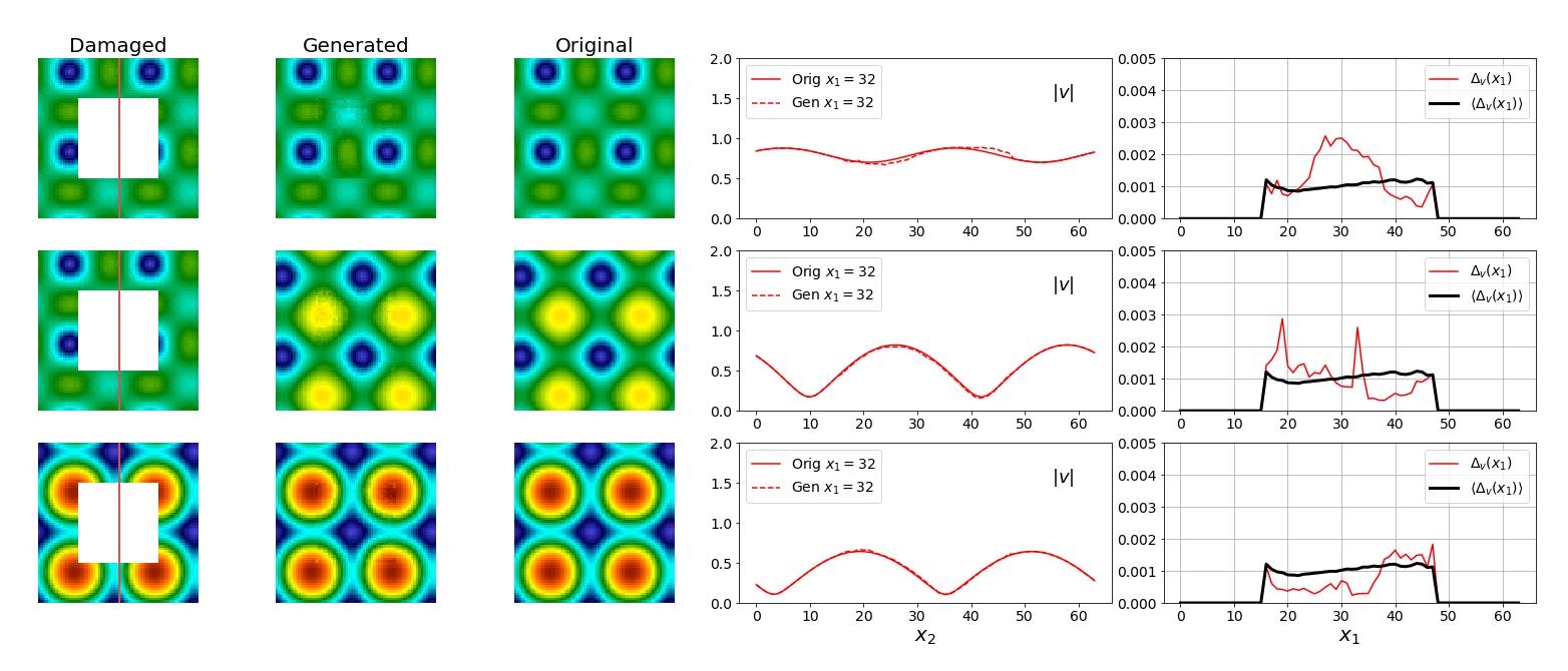
Figure 18: Benchmark of reconstruction on a 2d slice from a 3d random Taylor-Green flow. Interpolation is obtained with 1 part of one thousand precision in the whole region.

Appendix B CE2

As introduced in Sec. IV, the CE2 architecture is a GAN composed by a Generator plus an adversarial Discriminator network, as shown in Fig.19. The networks largely derive their structure from the VGG (and AlexNet) CNNs, which proved very successful in the ImageNet image classification. The initial part of VGG is made of a sequence of convolutions of filter size=3 and is the key ingredient to infer underlying structural features from 2D images. We tried variations of this schema changing the filter size to 3,4 or 5, retaining the best configuration, that is the one we propose. We started from the code in amos2016image , which is a python program using the TensorFlow library, with minor changes to adapt it to our dataset.

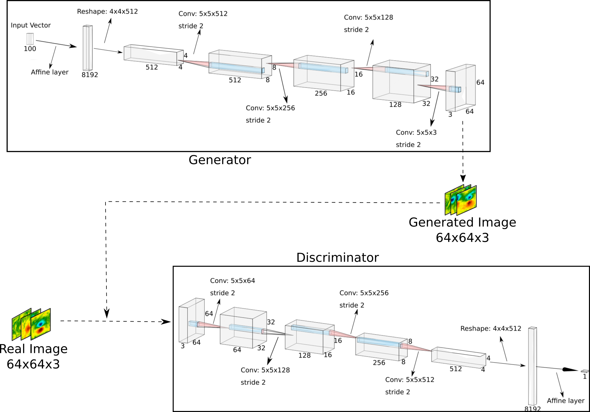
Figure 19: Structure of the CE2 network: the generator from a 100-dimensional input vector produces a 64x64x3 image, the discriminator decides if an input 64x64x3 image is coming from real data or is generated.

In detail, the generator part is a network aimed to produce a 3-dimensional velocity field starting from an arbitrary vector, ${\bf z}$, with $T$-real entries ($T=100$ in our implementation) which should prescribe the desired features. The feature size of 100 was chosen as a compromise between accuracy versus training time after attempts with $T=300,800,1000$ that did not improve the error in a significative way. This is in line with current impainting algorithms for images of similar input size. It is similar to the decoder part of the CE1, plus the insertion of a fully connected layer from the input to an intermediate layer of size $8192$ that then is reshaped as $4\times 4\times 512$ volume. The latter is used as the first stage of the next layers: with four successive transposed convolutions of size $5\times 5$ with stride=$2$ (with ReLu activation) we go from $4\times 4\times 512$ to $8\times 8\times 512$ to $16\times 16\times 256$ to $32\times 32\times 128$ to finally obtain, using $3$ transposed convolutions, the output velocity field of size $64\times 64\times 3$. The Discriminator network, takes a 3 component velocity field of dimension $64\times 64$ and outputs the probability that the input is real. Similar to the analogous in the CE1 network, using convolutional layers of size $5\times 5$ with stride=$2$ (with LeakyRELU activation) we reduce the dimension of the input down to a $4\times 4$ image with 512 channels. After reshaping to a vector of size $8192$, the last stage is made of a fully connected layer and a sigmoid activation function, providing the probability to be real or created by the generator.
The generator component of the network is trained to minimize the function:

$$\mathcal{L}_{gen}=\mathbb{E}_{{\bf z}}\{\log(1-D[G[{\bf z}]])\}$$ (16)

in order to fool the discriminator with its fake output. The discriminator component of the network is trained to maximize the function:

$$\mathcal{L}_{adv}=\mathbb{E}_{{\cal I}_{v},{\bf z}}\{\log(D[{\cal I}_{v}])+\log(1-D[G[{\bf z}]])\}$$ (17)

in order to assign probability $1$ to real fields and probability $0$ to generated fields. As with CE1, we have normalized independently the $3$ components of the input data to be in the $[-1:1]$ range. The Generator output was then re-scaled to match the original range of the velocity fields. Both networks are trained with the ADAM optimizer, kingma2014adam , using a learning rate of $2\times 10^{-4}$, $\beta_{1}=0.5$, $\beta_{2}=0.999$ and $\epsilon=10^{-8}$. The training was performed using a batch size equal to 256, so the $81\times 1024$ planes of the dataset were divided into 324 minibatches for a total of 100 Epochs. After the Deep-Gan is trained, its weights are frozen and used for the reconstruction phase: to recover the optimal ${\bf z}^{*}$-encoding that is closest to each corrupted image, the loss given in eq. 12 is minimized by back propagation to the input data using an ADAM optimization. In our test, we used a set of N=1024 images to be completed (selected outside the train dataset for the GAN), each minimized independently (batch size=1), with a learning rate of $2\times 10^{-2}$, $\beta_{1}=0.9$, $\beta_{2}=0.999$ and $\epsilon=10^{-8}$ for a high number of epochs (10 000).

Appendix C Database

Data are key for machine learning; hence, our aim to produce and curate benchmark datasets (and software) to foster interest among researchers in related fields. Complex flows and complex fluids benchmarks are more challenging than the traditional image datasets found in computer vision and machine learning: our data have high-resolution, multi-scale features, are inherently stochastic, without long term spatial and temporal correlations, and -often- with multi-scale non differentiable properties.
We share the believe that we are entering a new era in fluid mechanics research. Decades (centuries) of great theoretical, numerical and experimental developments based on first principles, brute-force simulations of the equations of motion or accurate observation of nature are now confronting with data-driven tools and analysis.
The database used is SMART-Rot a subset of data deployed in Smart-TURB turbrot and it is prepared in four steps:

• The DNS simulations at a resolution of $256^{3}$ grid points are truncated in Fourier space retaining till $k_{f}\leq 32$, then transformed back in real space downscaling them to $64^{3}$

• From the whole time evolution, a number of $600$ snapshots is used, with large temporal separation to decrease correlations (see Fig. 20).

• For each configuration, 16 horizontal cuts in the plane $(x_{1},x_{2})$ are selected. To increase the dataset, we shift each plane in $11$ different random ways such as to preserve periodic boundary conditions and to obtain a total of $16\times 11=176$ planes

• Finally, the dataset is composed of $600\times 176=105600$ planes, which are organized in a random order to avoid any time-correlation between successive planes.

Figure 20: Energy evolution for the turbulent flow generated during the simulation performed to generate the database of $600$ different configuration at a resolution of $256^{3}$ grid points. The velocity fields are extracted from time $t=276$, to reach the flow thermalization, up to the final time of $t=876$ every $t=1$ which corresponds to $2000$ simulation time-steps.

The database of the configurations was then divided into train set, the first $80\times 1024$ planes, and validation set, the next $20\times 1024$ planes.
The full database TURB-Rot is made public, available for download using the SMART-Turb portal turbrot . The portal uses the concept of "Dataset" to aggregate resources related to the same simulation: we have released both the original full resolution of 3d DNS snapshot at $256^{3}$ grid points and the database of $105600$ ($x_{1},x_{2}$)-planes with size $64\times 64$ used by CE1 and CE2, in a dataset named $\mathbf{TURB-Rot}$.

References

- [1] Roderick JA Little and Donald B Rubin. Statistical analysis with missing data, volume 793. John Wiley & Sons, 2019.
- [2] Mark Asch, Marc Bocquet, and Maëlle Nodet. Data assimilation: methods, algorithms, and applications, volume 11. SIAM, 2016.
- [3] Deepak Pathak, Philipp Krahenbuhl, Jeff Donahue, Trevor Darrell, and Alexei A Efros. Context encoders: Feature learning by inpainting. In Proceedings of the IEEE conference on computer vision and pattern recognition, pages 2536–2544, 2016.
- [4] Raymond A Yeh, Chen Chen, Teck Yian Lim, Alexander G Schwing, Mark Hasegawa-Johnson, and Minh N Do. Semantic image inpainting with deep generative models. In Proceedings of the IEEE conference on computer vision and pattern recognition, pages 5485–5493, 2017.
- [5] Dmitry Ulyanov, Andrea Vedaldi, and Victor Lempitsky. Deep image prior. In Proceedings of the IEEE Conference on Computer Vision and Pattern Recognition, pages 9446–9454, 2018.
- [6] Tomas Mikolov, Ilya Sutskever, Kai Chen, Greg S Corrado, and Jeff Dean. Distributed representations of words and phrases and their compositionality. In Advances in neural information processing systems, pages 3111–3119, 2013.
- [7] Samuel R Bowman, Gabor Angeli, Christopher Potts, and Christopher D Manning. A large annotated corpus for learning natural language inference. arXiv:1508.05326, 2015.
- [8] Qi Wang, Yosuke Hasegawa, and Tamer A. Zaki. Spatial reconstruction of steady scalar sources from remote measurements in turbulent flow. Journal of Fluid Mechanics, 870:316–352, July 2019. Publisher: Cambridge University Press.
- [9] Vincent Mons, Qi Wang, and Tamer A. Zaki. Kriging-enhanced ensemble variational data assimilation for scalar-source identification in turbulent environments. Journal of Computational Physics, 398:108856, December 2019.
- [10] Eugenia Kalnay. Atmospheric Modeling, Data Assimilation and Predictability. Cambridge University Press, 2003.
- [11] Markus Reichstein, Gustau Camps-Valls, Bjorn Stevens, Martin Jung, Joachim Denzler, Nuno Carvalhais, et al. Deep learning and process understanding for data-driven earth system science. Nature, 566(7743):195–204, 2019.
- [12] Alberto Carrassi, Marc Bocquet, Laurent Bertino, and Geir Evensen. Data assimilation in the geosciences: An overview of methods, issues, and perspectives. Wiley Interdisciplinary Reviews: Climate Change, 9(5):e535, 2018.
- [13] Peter Bauer, Alan Thorpe, and Gilbert Brunet. The quiet revolution of numerical weather prediction. Nature, 525(7567):47–55, 2015.
- [14] Jia Deng, Wei Dong, Richard Socher, Li-Jia Li, Kai Li, and Li Fei-Fei. Imagenet: A large-scale hierarchical image database. In 2009 IEEE conference on computer vision and pattern recognition, pages 248–255. Ieee, 2009.
- [15] Li Deng. The mnist database of handwritten digit images for machine learning research. IEEE Signal Processing Magazine, 29(6):141–142, 2012.
- [16] Alex Krizhevsky, Ilya Sutskever, and Geoffrey E Hinton. Imagenet classification with deep convolutional neural networks. In Advances in neural information processing systems, pages 1097–1105, 2012.
- [17] Ziwei Liu, Ping Luo, Xiaogang Wang, and Xiaoou Tang. Deep learning face attributes in the wild. In Proceedings of the IEEE international conference on computer vision, pages 3730–3738, 2015.
- [18] Yuval Netzer, Tao Wang, Adam Coates, Alessandro Bissacco, Bo Wu, and Andrew Y. Ng. Reading digits in natural images with unsupervised feature learning. In NIPS Workshop on Deep Learning and Unsupervised Feature Learning 2011, 2011.
- [19] Jonathan Krause, Michael Stark, Jia Deng, and Li Fei-Fei. 3d object representations for fine-grained categorization. In Proceedings of the IEEE international conference on computer vision workshops, pages 554–561, 2013.
- [20] Cristian C. Lalescu, Charles Meneveau, and Gregory L. Eyink. Synchronization of chaos in fully developed turbulence. Phys. Rev. Lett., 110:084102, Feb 2013.
- [21] Luca Biferale, Fabio Bonaccorso, Michele Buzzicotti, and Patricio Clark di Leoni. TURB-Rot. A large database of 3d and 2d snapshots from turbulent rotating flows. http://smart-turb.roma2.infn.it. arXiv:2006.07469, 2020.
- [22] Alexandros Alexakis and Luca Biferale. Cascades and transitions in turbulent flows. Physics Reports, 767:1–101, 2018.
- [23] Uriel Frisch. Turbulence: the legacy of AN Kolmogorov. Cambridge University Press, 1995.
- [24] A. P. McNally and P. D. Watts. A cloud detection algorithm for high-spectral-resolution infrared sounders. Quarterly Journal of the Royal Meteorological Society, 129(595):3411–3423, 2003. _eprint: https://rmets.onlinelibrary.wiley.com/doi/pdf/10.1256/qj.02.208.
- [25] Peter Bauer, Alan J. Geer, Philippe Lopez, and Deborah Salmond. Direct 4D-Var assimilation of all-sky radiances. Part I: Implementation. Quarterly Journal of the Royal Meteorological Society, 136(652):1868–1885, 2010. _eprint: https://rmets.onlinelibrary.wiley.com/doi/pdf/10.1002/qj.659.
- [26] James E. Hoke and Richard A. Anthes. The initialization of numerical models by a dynamic-initialization technique. Monthly Weather Review, 104(12):1551–1556, 1976.
- [27] S. Lakshmivarahan and John M. Lewis. Nudging methods: A critical overview. In Data Assimilation for Atmospheric, Oceanic and Hydrologic Applications (Vol. II), pages 27–57. Springer, Berlin, Heidelberg, 2013.
- [28] Patricio Clark Di Leoni, Andrea Mazzino, and Luca Biferale. Synchronization to Big Data: Nudging the Navier-Stokes Equations for Data Assimilation of Turbulent Flows. Physical Review X, 10(1):011023, February 2020. Publisher: American Physical Society.
- [29] Gal Berkooz, Philip Holmes, and John L Lumley. The proper orthogonal decomposition in the analysis of turbulent flows. Annual review of fluid mechanics, 25(1):539–575, 1993.
- [30] Steven L Brunton and J Nathan Kutz. Data-driven science and engineering: Machine learning, dynamical systems, and control. Cambridge University Press, 2019.
- [31] Thomas Duriez, Steven L Brunton, and Bernd R Noack. Machine learning control-taming nonlinear dynamics and turbulence, volume 116. Springer, 2017.
- [32] Steven L Brunton, Bernd R Noack, and Petros Koumoutsakos. Machine learning for fluid mechanics. Annual Review of Fluid Mechanics, 52:477–508, 2020.
- [33] Kai Fukami, Koji Fukagata, and Kunihiko Taira. Super-resolution reconstruction of turbulent flows with machine learning. Journal of Fluid Mechanics, 870:106–120, July 2019.
- [34] Kai Fukami, Yusuke Nabae, Ken Kawai, and Koji Fukagata. Synthetic turbulent inflow generator using machine learning. Physical Review Fluids, 4(6):064603, June 2019. arXiv: 1806.08903.
- [35] Jared L. Callaham, Kazuki Maeda, and Steven L. Brunton. Robust flow reconstruction from limited measurements via sparse representation. Physical Review Fluids, 4(10):103907, October 2019.
- [36] Maziar Raissi, Alireza Yazdani, and George Em Karniadakis. Hidden fluid mechanics: Learning velocity and pressure fields from flow visualizations. Science, 367(6481):1026–1030, February 2020. Publisher: American Association for the Advancement of Science Section: Report.
- [37] Julien Brajard, Alberto Carrassi, Marc Bocquet, and Laurent Bertino. Combining data assimilation and machine learning to emulate a dynamical model from sparse and noisy observations: a case study with the Lorenz 96 model. Geoscientific Model Development Discussions, pages 1–21, May 2019.
- [38] Alexander Wikner, Jaideep Pathak, Brian Hunt, Michelle Girvan, Troy Arcomano, Istvan Szunyogh, Andrew Pomerance, and Edward Ott. Combining machine learning with knowledge-based modeling for scalable forecasting and subgrid-scale closure of large, complex, spatiotemporal systems. Chaos: An Interdisciplinary Journal of Nonlinear Science, 30(5):053111, 2020.
- [39] Maziar Raissi, Paris Perdikaris, and George E Karniadakis. Physics-informed neural networks: A deep learning framework for solving forward and inverse problems involving nonlinear partial differential equations. Journal of Computational Physics, 378:686–707, 2019.
- [40] Jin-Long Wu, Karthik Kashinath, Adrian Albert, Dragos Chirila, Heng Xiao, et al. Enforcing statistical constraints in generative adversarial networks for modeling chaotic dynamical systems. Journal of Computational Physics, 406:109209, 2020.
- [41] Rui Wang, Adrian Albert, Karthik Kashinath, and Mustafa Mustafa. Towards physics-informed deep learning for spatiotemporal modeling of turbulent flows. AGUFM, 2019:IN32B–13, 2019.
- [42] N Benjamin Erichson, Michael Muehlebach, and Michael W Mahoney. Physics-informed autoencoders for lyapunov-stable fluid flow prediction. arXiv:1905.10866, 2019.
- [43] Bethany Lusch, J Nathan Kutz, and Steven L Brunton. Deep learning for universal linear embeddings of nonlinear dynamics. Nature communications, 9(1):1–10, 2018.
- [44] Karthik Kashinath, Philip Marcus, et al. Enforcing physical constraints in cnns through differentiable pde layer. In ICLR 2020 Workshop on Integration of Deep Neural Models and Differential Equations, 2020.
- [45] Arvind T Mohan, Nicholas Lubbers, Daniel Livescu, and Michael Chertkov. Embedding hard physical constraints in convolutional neural networks for 3d turbulence. In ICLR 2020 Workshop on Integration of Deep Neural Models and Differential Equations, 2020.
- [46] Arvind Mohan, Don Daniel, Michael Chertkov, and Daniel Livescu. Compressed convolutional lstm: An efficient deep learning framework to model high fidelity 3d turbulence. arXiv:1903.00033, 2019.
- [47] Steffen Wiewel, Moritz Becher, and Nils Thuerey. Latent space physics: Towards learning the temporal evolution of fluid flow. In Computer Graphics Forum, volume 38,2, pages 71–82. Wiley Online Library, 2019.
- [48] Byungsoo Kim, Vinicius C Azevedo, Nils Thuerey, Theodore Kim, Markus Gross, and Barbara Solenthaler. Deep fluids: A generative network for parameterized fluid simulations. In Computer Graphics Forum, volume 38,2, pages 59–70. Wiley Online Library, 2019.
- [49] Liu Yang, Sean Treichler, Thorsten Kurth, Keno Fischer, David Barajas-Solano, Josh Romero, Valentin Churavy, Alexandre Tartakovsky, Michael Houston, Prabhat, and George Karniadakis. Highly-scalable, physics-informed GANs for learning solutions of stochastic PDEs. arXiv:1910.13444 [physics, stat], October 2019. arXiv: 1910.13444.
- [50] Geir Evensen. Data Assimilation: The Ensemble Kalman Filter. Springer Science & Business Media, 2006.
- [51] P. L. Houtekamer and Fuqing Zhang. Review of the ensemble kalman filter for atmospheric data assimilation. Monthly Weather Review, 144(12):4489–4532, 2016.
- [52] Michael L Stein. Interpolation of spatial data: some theory for kriging. Springer Science & Business Media, 2012.
- [53] Hasan Gunes, Sirod Sirisup, and George Em Karniadakis. Gappy data: To krig or not to krig? Journal of Computational Physics, 212(1):358–382, 2006.
- [54] Daniele Venturi and George Em Karniadakis. Gappy data and reconstruction procedures for flow past a cylinder. Journal of Fluid Mechanics, 519:315–336, 2004.
- [55] Isabel Scherl, Benjamin Strom, Jessica K Shang, Owen Williams, Brian L Polagye, and Steven L Brunton. Robust principal component analysis for modal decomposition of corrupt fluid flows. Physical Review Fluids, 5(5):054401, 2020.
- [56] Nathan E Murray and Lawrence S Ukeiley. An application of gappy pod. Experiments in Fluids, 42(1):79–91, 2007.
- [57] Carola-Bibiane Schönlieb. Partial differential equation methods for image inpainting, volume 29. Cambridge University Press, 2015.
- [58] Marcelo Bertalmio, Andrea L Bertozzi, and Guillermo Sapiro. Navier-stokes, fluid dynamics, and image and video inpainting. In Proceedings of the 2001 IEEE Computer Society Conference on Computer Vision and Pattern Recognition. CVPR 2001, volume 1, pages I–I. IEEE, 2001.
- [59] MA Ebrahimi and Evelyn Lunasin. The navier–stokes–voight model for image inpainting. The IMA Journal of Applied Mathematics, 78(5):869–894, 2013.
- [60] Peter Alan Davidson. Turbulence in rotating, stratified and electrically conducting fluids. Cambridge University Press, 2013.
- [61] Antoine Campagne, Basile Gallet, Frédéric Moisy, and Pierre-Philippe Cortet. Direct and inverse energy cascades in a forced rotating turbulence experiment. Physics of Fluids, 26(12):125112, 2014.
- [62] Annick Pouquet and Raffaele Marino. Geophysical turbulence and the duality of the energy flow across scales. Physical review letters, 111(23):234501, 2013.
- [63] Ehud Yarom and Eran Sharon. Experimental observation of steady inertial wave turbulence in deep rotating flows. Nature Physics, 10(7):510–514, 2014.
- [64] Pierre Sagaut and Claude Cambon. Homogeneous turbulence dynamics, volume 10. Springer, 2008.
- [65] Michele Buzzicotti, Hussein Aluie, Luca Biferale, and Moritz Linkmann. Energy transfer in turbulence under rotation. Physical Review Fluids, 3(3):034802, 2018.
- [66] Luca Biferale, Fabio Bonaccorso, Irene M Mazzitelli, Michel AT van Hinsberg, Alessandra S Lanotte, Stefano Musacchio, Prasad Perlekar, and Federico Toschi. Coherent structures and extreme events in rotating multiphase turbulent flows. Physical Review X, 6(4):041036, 2016.
- [67] Leslie M Smith and Fabian Waleffe. Transfer of energy to two-dimensional large scales in forced, rotating three-dimensional turbulence. Physics of fluids, 11(6):1608–1622, 1999.
- [68] Nitish Srivastava, Geoffrey Hinton, Alex Krizhevsky, Ilya Sutskever, and Ruslan Salakhutdinov. Dropout: a simple way to prevent neural networks from overfitting. The journal of machine learning research, 15(1):1929–1958, 2014.
- [69] Marcelo Bertalmio, Guillermo Sapiro, Vincent Caselles, and Coloma Ballester. Image inpainting. In Proceedings of the 27th annual conference on Computer graphics and interactive techniques, pages 417–424, 2000.
- [70] Connelly Barnes, Eli Shechtman, Adam Finkelstein, and Dan B Goldman. Patchmatch: A randomized correspondence algorithm for structural image editing. In ACM Transactions on Graphics (ToG), volume 28,3, page 24. ACM, 2009.
- [71] Alexei A Efros and Thomas K Leung. Texture synthesis by non-parametric sampling. In Proceedings of the seventh IEEE international conference on computer vision, volume 2, pages 1033–1038. IEEE, 1999.
- [72] Stanley Osher, Martin Burger, Donald Goldfarb, Jinjun Xu, and Wotao Yin. An iterative regularization method for total variation-based image restoration. Multiscale Modeling & Simulation, 4(2):460–489, 2005.
- [73] Stephen B. Pope. Turbulent Flows. Cambridge University Press, 2000.
- [74] C. Meneveau and J. Katz. Scale-invariance and turbulence models for large-eddy simulation. Ann. Rev. Fluid Mech., 32:1, 2000.
- [75] Ian Goodfellow, Jean Pouget-Abadie, Mehdi Mirza, Bing Xu, David Warde-Farley, Sherjil Ozair, Aaron Courville, and Yoshua Bengio. Generative adversarial nets. In Advances in neural information processing systems, pages 2672–2680, 2014.
- [76] Emily L Denton, Soumith Chintala, Rob Fergus, et al. Deep generative image models using a laplacian pyramid of adversarial networks. In Advances in neural information processing systems, pages 1486–1494, 2015.
- [77] Karen Simonyan, Andrea Vedaldi, and Andrew Zisserman. Deep inside convolutional networks: Visualising image classification models and saliency maps. arXiv:1312.6034, 2013.
- [78] Shlomo Benartzi, John Beshears, Katherine L Milkman, Cass R Sunstein, Richard H Thaler, Maya Shankar, Will Tucker-Ray, William J Congdon, and Steven Galing. Should governments invest more in nudging? Psychological science, 28(8):1041–1055, 2017.
- [79] Masakazu Gesho, Eric Olson, and Edriss S. Titi. A Computational Study of a Data Assimilation Algorithm for the Two-dimensional Navier-Stokes Equations. Communications in Computational Physics, 19(4):1094–1110, April 2016.
- [80] Aseel Farhat, Evelyn Lunasin, and Edriss S. Titi. Abridged Continuous Data Assimilation for the 2d Navier–Stokes Equations Utilizing Measurements of Only One Component of the Velocity Field. Journal of Mathematical Fluid Mechanics, 18(1):1–23, March 2016.
- [81] A Farhat, NE Glatt-Holtz, VR Martinez, SA McQuarrie, and JP Whitehead. Data assimilation in large prandtl rayleigh–bénard convection from thermal measurements. SIAM Journal on Applied Dynamical Systems, 19(1):510–540, 2020.
- [82] Patricio Clark Di Leoni, Andrea Mazzino, and Luca Biferale. Inferring flow parameters and turbulent configuration with physics-informed data assimilation and spectral nudging. Physical Review Fluids, 3(10):104604, 2018.
- [83] Suraj Pawar, Shady E Ahmed, Omer San, Adil Rasheed, and Ionel M Navon. Long short-term memory embedded nudging schemes for nonlinear data assimilation of geophysical flows. arXiv:2005.11296, 2020.
- [84] Marc T Henry de Frahan and Ray W Grout. Data recovery in computational fluid dynamics through deep image priors. arXiv:1901.11113, 2019.
- [85] Jianhong Shen and Tony F Chan. Mathematical models for local nontexture inpaintings. SIAM Journal on Applied Mathematics, 62(3):1019–1043, 2002.
- [86] Holger Nobach and Eberhard Bodenschatz. Limitations of accuracy in piv due to individual variations of particle image intensities. Experiments in fluids, 47(1):27–38, 2009.
- [87] Shuiwang Ji, Wei Xu, Ming Yang, and Kai Yu. 3d convolutional neural networks for human action recognition. IEEE transactions on pattern analysis and machine intelligence, 35(1):221–231, 2012.
- [88] Okan Köpüklü, Neslihan Kose, Ahmet Gunduz, and Gerhard Rigoll. Resource efficient 3d convolutional neural networks. arXiv:1904.02422, 2019.
- [89] Martín Abadi, Ashish Agarwal, Paul Barham, Eugene Brevdo, Zhifeng Chen, Craig Citro, Greg S. Corrado, Andy Davis, Jeffrey Dean, Matthieu Devin, Sanjay Ghemawat, Ian Goodfellow, Andrew Harp, Geoffrey Irving, Michael Isard, Yangqing Jia, Rafal Jozefowicz, Lukasz Kaiser, Manjunath Kudlur, Josh Levenberg, Dandelion Mané, Rajat Monga, Sherry Moore, Derek Murray, Chris Olah, Mike Schuster, Jonathon Shlens, Benoit Steiner, Ilya Sutskever, Kunal Talwar, Paul Tucker, Vincent Vanhoucke, Vijay Vasudevan, Fernanda Viégas, Oriol Vinyals, Pete Warden, Martin Wattenberg, Martin Wicke, Yuan Yu, and Xiaoqiang Zheng. TensorFlow: Large-scale machine learning on heterogeneous systems, 2015. Software available from tensorflow.org.
- [90] Alexander LeNail. Nn-svg: Publication-ready neural network architecture schematics. Journal of Open Source Software, 4(33):747, 2019.
- [91] Diederik P Kingma and Jimmy Ba. Adam: A method for stochastic optimization. arXiv:1412.6980, 2014.
- [92] Brandon Amos. Image Completion with Deep Learning in TensorFlow. http://bamos.github.io/2016/08/09/deep-completion. Accessed: 2019.