Direct Vlasov solvers

Abstract

In these proceedings we will describe the theory and practical steps required to build Vlasov solvers such as those commonly used to compute coherent instabilities in synchrotrons. Thanks to a Hamiltonian formalism, we will derive a compact and general form of the linearized Vlasov equation, written using Poisson brackets. This in turn will be the basis of a procedure to build Vlasov solvers, applied to the specific example of transverse instabilities arising from beam coupling impedance.

0.1 Introduction

In particle accelerators and storage rings, beam quality is sometimes affected by so-called ‘collective effects’, which can lead to e.g. emittance growth or intensity loss. These effects are characterized by various kinds of interactions between beam particles, building up to a collective behaviour of the ensemble of particles which fundamentally differs from that of a set of independent particles.

Several such collective effects can lead to coherent instabilities in which the beam average position exhibits self-enhanced, growing oscillations. These can ultimately lead to a significant decrease of the beam brightness, or even a complete loss of the beam in the worst case, and are a source of limitation to the operation of particle accelerators. For instance, the transverse instabilities observed in the Large Hadron Collider (LHC) during run I and II at top energy, led to the use of very high current in the octupolar magnets (close to the maximum available) to provide enough Landau damping [ref:EMetral_summary_LHC_instab_review_runI, ref:EMetral_summary_LHC_instab_review_runII]. Other examples of limitations due to beam instabilities in hadron synchrotrons were reviewed in Refs. [ref:IEEE, ref:Salvant_Benevento].

Coherent instabilities can be caused by various kinds of collective effects (or a combination of several of them):

• beam-coupling impedance, i.e. self-generated electromagnetic fields obtained through the interaction between the beam and its surroundings (vacuum pipe, kickers, collimators, cavities, etc.),

• an electron cloud around the beam, due to secondary emission of electrons at the surface surrounding the beam,

• interactions with ions trapped in the beam potential,

• beam-beam effects, i.e. interaction with a counter-rotating beam.

There are essentially two common ways to model such interactions:

• macroparticle simulations (or indirect Vlasov solvers): the beam is looked as a collection of macroparticles which are tracked down the full ring. Both the machine optics and the particle interactions are included in the dynamics of each macroparticle, in an attempt to be as realistic as possible. The goal is to observe directly the time evolution of the beam transverse motion and hence spot possible instabilities. The number of macroparticles is still typically much smaller than the number of actual particles,

• direct Vlasov solvers (hereafter simply named Vlasov solvers): the phase space distribution is modelled as a continuum rather than a collection of discrete particles, and Vlasov equation is solved.

Historically, the latter approach was the first adopted to try to understand the instabilities observed in particle accelerators [ref:Laslett, ref:Sacherer1972]. More recently, macroparticles simulations have been used extensively and have shown their capabilities to model the beam behaviour in complex situations. Tracking macroparticles through such simulations is indeed efficient, often extensible at will to almost any kind of particle interactions, and potentially very close to reality. We refer the reader to Ref. [ref:Kli] for a detailed review of macroparticles simulations and their numerical implementation.

Despite its success in many aspects, this approach may still suffer from two possibly important limitations. First, it is a pure time domain technique, and simulations need to be stopped after tracking a certain number of turns. Therefore, slow instabilities can be missed, and these can be critical in some machines where the beam remains stored for a very long time (hours, in the case of the LHC). Second, such simulations do not necessarily provide a synthetic understanding of the kind of instability, neither of the main parameters nor mitigation means that could prevent it, unless large and computationally intensive parameter scans are performed.

Vlasov solvers, on the contrary, are typically limited to simpler situations, but can provide a good understanding of instability modes and their mitigation parameters. Moreover, they are typically very fast. Finally, they are in principle able to spot an instability irrespectively of its rapidity to develop.

For more detailed reviews on the two approaches and comparisons between them, the reader is referred to Refs. [ref:Migliorati, ref:KLi_MSchenk, ref:Mounet_Benevento]. Here we will focus on direct Vlasov solvers only, both from the theoretical and the practical point of view.

The three main sections of these proceedings are rather independent from each other. In Section 0.2 we will introduce the concept of phase space distribution density and provide Vlasov equation. In Section 0.3 we obtain the linearized form of this equation in a compact way, eq:linear_Vlasov, as well as higher order extensions, thanks to Poisson brackets and a Hamiltonian formalism. The core of these proceedings will then be given in Section LABEL:sec:method, where a method to build a Vlasov solver will be described through its application to the specific case of transverse instabilities resulting from beam-coupling impedance, for a bunched beam. Finally, we will conclude in Section LABEL:sec:conclusion.

0.2 Vlasov equation

In this section we will introduce Vlasov equation and briefly review existing Vlasov solvers. Many more details can be found in Ref. [ref:Chen] in the context of plasma physics in general, and in Ref. [ref:Chao, chap. 6] for the specific case of impedance effects in beam physics.

0.2.1 Particle distribution in phase space

In a classical picture (i.e. neglecting quantum-mechanical effects), each beam particle has a well defined position and momentum in phase space for each of the three coordinates $(x,y,z)$. The distribution function $\psi$ then represents the density of particles in the six-dimensional (6D) phase space. In fig:distributions we sketch examples of such particles distributions, represented here in one plane only.

The number of particles in a given phase space volume $V$ is then obtained from the 6D integral

$$\mathcal{N}(V)=\iiint\iiint_{V}\mathrm{d}x\mathrm{d}y\mathrm{d}z\,\mathrm{d}p_{x}\mathrm{d}p_{y}\mathrm{d}p_{z}\;\psi\left(x,y,z,p_{x},p_{y},p_{z}\right),$$ (1)

which gives the total number of particles $N$ when $V$ is the full phase space. The average value of any function $f$ of the particle positions and momenta, over a phase space volume $V$, is similarly given by

$$\left<f\left(V\right)\right>=\iiint\iiint_{V}\mathrm{d}x\mathrm{d}y\mathrm{d}z\,\mathrm{d}p_{x}\mathrm{d}p_{y}\mathrm{d}p_{z}\;f\left(x,y,z,p_{x},p_{y},p_{z}\right)\psi\left(x,y,z,p_{x},p_{y},p_{z}\right).$$ (2)

In the case of an ensemble of particles evolving with time, $\psi$ also depends on the time $t$.

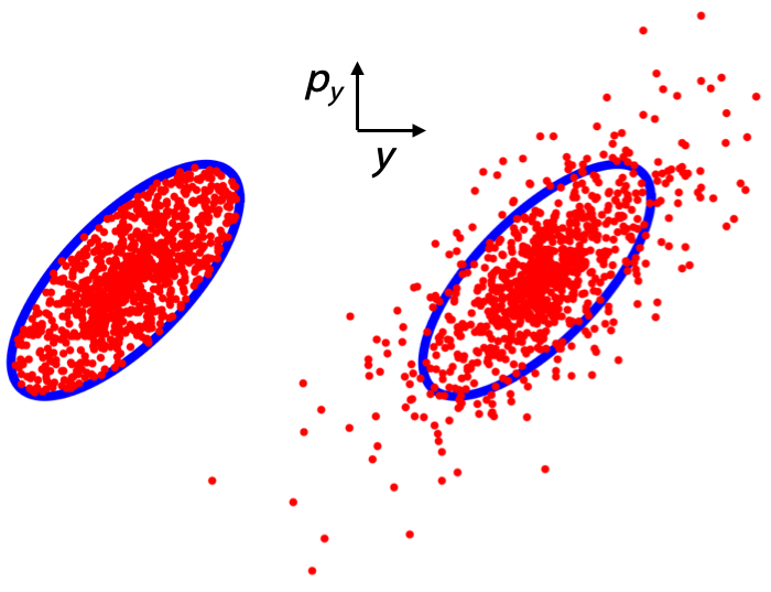
Figure 1: Uniform (left) and Gaussian (right) distributions of particles in phase space, projected on the vertical plane $(y,p_{y})$. The ellipse contains all the particles of the uniform distribution, and 80% of them for the Gaussian case.

0.2.2 From Liouville theorem to Vlasov equation

In a collisionless Hamiltonian system, Liouville’s theorem states that the distribution function is constant along any trajectory in phase space. This means that the local phase space distribution function does not change when one follows the flow (i.e. the trajectory) of particles. This is illustrated in fig:Liouville: time evolution makes the square evolve into a parallelogram of same area, containing the same number of particles as the initial square, hence the average density will be the same.

Mathematically, this theorem can be expressed by stating that the total time derivative of the distribution function is zero at any time, i.e.

$$\frac{d\psi}{dt}=0.$$ (3)

Liouville’s theorem applies in principle to a system of non-colliding (i.e. non-interacting) particles – it is actually equivalent to the collisionless Boltzmann transport equation. For a plasma such as a beam of particles in a synchrotron, one could think of the particle electromagnetic (EM) interactions as Coulomb collisions in the rest frame of the beam, hence rather intuitively use a collision-based Boltzmann equation, with Coulomb interactions added as a collision term, rather than Liouville’s theorem. In the early days of plasma physics, this approach turned out not to be successful, essentially because of the long-range character of electromagnetic interactions. A much better approach, found by Vlasov [ref:Vlasov_in_Russian, ref:Vlasov], was instead to integrate the collective, self-interaction EM fields into the Hamiltonian itself. This gave birth to Vlasov equation which is simply the expression of eq:Liouville for a plasma under the action of its own EM fields.

The only assumptions for the Vlasov equation are therefore:

• the system is Hamiltonian; in particular, there is no damping or diffusion mechanism due to external sources ,

• particles are interacting only through the collective EM fields (no short-range collisions),

• there is no creation nor annihilation of particles.

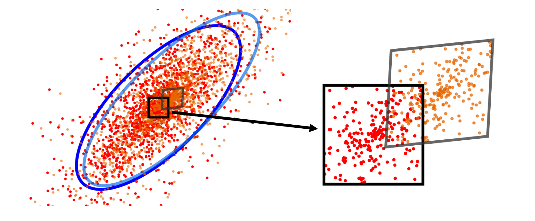
Figure 2: Example of time evolution of a Gaussian distribution of particles. Red particles at time $t$ become the orange ones at time $t+dt$, and the associated dark blue ellipse (resp. the black square) becomes the light blue one (resp. the grey parallelogram).

0.2.3 A short review of existing Vlasov solvers

Vlasov solvers have been theorized and implemented since as early as 1965 with the pioneer work of Laslett et al [ref:Laslett]. They can be used for various kinds of collective effects involving self-generated EM fields:

• beam-beam effects [ref:Chao1984, ref:Alexahin],

• electron-cloud (and more generally two-stream effects) [ref:Perevedentsev, ref:Davidson],

• space-charge[ref:Ryne],

• combined effect of impedance and space-charge [ref:Blaskiewicz, ref:Burov, ref:Balbekov, ref:Shobuda],

• longitudinal impedance [ref:Venturini, ref:Lindberg_longitudinal],

• transverse impedance [ref:Laslett, ref:Sacherer1972, ref:Sacherer1974, ref:Zotter_EMajorana, ref:Sacherer_EMajorana, ref:Besnier1979, ref:Besnier1984, ref:Chin_LandauDamping, ref:Laclare, ref:JSBerg, ref:KarlinerPopov, ref:Lindberg, ref:Schenk].

For impedance-related instabilities, a number of codes are available, implementing Vlasov solvers in longitudinal — e.g. GALACLIC (GArnier-LAclare Coherent Longitudinal Instabilities Code) [ref:EMetral_GALACTIC_GALACLIC], as well as in transverse — e.g. MOSES (MOde-coupling Single bunch instability in an Electron Storage ring) [ref:MOSES1, ref:MOSES2], NHTVS (Nested Head-Tail Vlasov Solver) [ref:NHTVS], DELPHI (Discrete Expansion over Laguerre Polynomials and Head-tail modes to compute Instabilities) [ref:Mounet_Benevento], and GALACTIC (GArnier-LAclare Coherent Transverse Instabilities Code) [ref:EMetral_GALACTIC, ref:EMetral_GALACTIC_GALACLIC].

0.3 Linearized Vlasov equation

After short introductions on Hamiltonians, canonical transformations and Poisson brackets, we will present in this section the basics of perturbation theory applied to Vlasov equation. A general linearized version of Vlasov equation will be derived, as done in Ref. [ref:KLi_Vlasov]. Higher order extensions are then also obtained.

0.3.1 Hamiltonian formalism

We consider the coordinates $(x,y,z)$ of a particle relative to a reference particle — called the synchronous particle — which travels along the synchrotron orbit at exactly the design velocity $v=\beta c$, with $\beta$ the relativistic velocity factor and $c$ the speed of light, such that its longitudinal position along the orbit is $s=vt$. In this reference system the synchronous particle has therefore positions $(x=0,y=0,z=0)$. $z$ is tangential to the orbit, and $(x,y)$ perpendicular to $z$, with $x$ in the plane of the orbit and directed towards the outside. We adopt here essentially the conventions and most of the notations of Ref. [ref:Chao, chap. 1].

The beam particles are solely affected by electromagnetic forces and constitute therefore a Hamiltonian system. In general the Hamiltonian is defined as the Legendre transform of the Lagrangian, which itself is the difference between the kinetic energy and the potential energy of the system. We will state without proof that the Hamiltonian corresponds to the sum of the kinetic and potential energy, and refer the reader to Ref. [ref:Goldstein] for more details on classical Hamiltonian mechanics, and to Refs. [ref:Bell, ref:Ruth_Hamiltonian, ref:Herr] for a detailed description of Hamiltonian dynamics applied to single particle beam physics.

The single-particle dynamics will be here expressed thanks to an effective Hamiltonian [ref:Herr] defined in general as a function of all the phase space coordinates and time

$$H\left(x,x^{\prime},y,y^{\prime},z,\delta;t\right),$$ (4)

with

$$x^{\prime}\equiv\frac{dx}{ds},\qquad y^{\prime}\equiv\frac{dy}{ds},\qquad\delta\equiv\frac{\Delta p_{z}}{p_{0}},$$ (5)

where $\Delta p_{z}$ is the deviation of the longitudinal momentum from that of the synchronous particle given by

$$p_{0}=m_{0}\gamma v,$$

$m_{0}$ being the rest mass and

$$\gamma=\sqrt{\frac{1}{1-\beta^{2}}}$$

the relativistic mass factor.

The time evolution is governed by Hamilton’s equations. In general, for any conjugate pair of position and momentum coordinates $(x_{i},p_{i})$, these are written

$$\frac{dx_{i}}{dt}=\frac{\partial H}{\partial p_{i}},\qquad\frac{dp_{i}}{dt}=-\frac{\partial H}{\partial x_{i}}.$$ (6)

In our case, Hamilton’s equations read