THE LIMITS OF MIN-MAX OPTIMIZATION ALGORITHMS:
CONVERGENCE TO SPURIOUS NON-CRITICAL SETS

Abstract.

Compared to ordinary function minimization problems, min-max optimization algorithms encounter far greater challenges because of the existence of periodic cycles and similar phenomena. Even though some of these behaviors can be overcome in the convex-concave regime, the general case is considerably more difficult. On that account, we take an in-depth look at a comprehensive class of state-of-the art algorithms and prevalent heuristics in non-convex / non-concave problems, and we establish the following general results: itn) generically, the algorithms’ limit points are contained in the internally chain-transitive (ICT) sets of a common, mean-field system; itn) the attractors of this system also attract the algorithms in question with arbitrarily high probability; and itn) all algorithms avoid the system’s unstable sets with probability $1$. On the surface, this provides a highly optimistic outlook for min-max algorithms; however, we show that there exist spurious attractors that do not contain any stationary points of the problem under study. In this regard, our work suggests that existing min-max algorithms may be subject to inescapable convergence failures. We complement our theoretical analysis by illustrating such attractors in simple, two-dimensional, almost bilinear problems.

1. Introduction

Consider a min-max optimization – or saddle-point – problem of the form

$$\min_{x\in\mathcal{X}}\max_{y\in\mathcal{Y}}\Phi(x,y).$$ (SP)

Given an algorithm for solving (SP), it is then natural to ask:

Where does the algorithm converge to? ($$\star$$)

The goal of our paper is to treat ($\star$ ‣ 1) in a general non-convex / non-concave setting and to provide answers for a comprehensive array of state-of-the-art algorithms.

Related work.

This question has attracted significant interest in the machine learning literature because of its potential implications to generative adversarial networks [32], robust reinforcement learning [74], and other models of adversarial training [56]. In this broad setting, it has become empirically clear that the joint training of two neural networks is fundamentally more difficult than that of a single NN of similar size and architecture. The latter task boils down to successfully finding a (good) local minimum of a non-convex function, so it is instructive to revisit ($\star$ ‣ 1) in the context of non-convex minimization.

In this case, the existing convergence theory for stochastic gradient descent (SGD) – the “gold standard” for deep NN training – can be informally summed up as follows:

1. stochastic gradient descent (SGD) always converges to critical points.

2. SGD does not converge to strict saddle points or other spurious solutions.

These results could be seen as plausible expectations for algorithmic proposals to solve (SP). Unfortunately however, there are well-known examples of simple bilinear min-max games where stochastic gradient descent/ascent (SGDA), the min-max analogue of SGD, leads to recurrent orbits that do not contain any critical point of $\Phi$. Such spurious convergence phenomena arise from the min-max structure of (SP) and have no counterpart in minimization problems.

This well-documented failure of SGDA has led to an extensive literature that is impossible to survey here. As a purely indicative – and highly incomplete – list, we mention the works of Daskalakis et al [21], Gidel et al [30], Mertikopoulos et al [59] and Mokhtari et al [62], who studied how these failures can be overcome in deterministic bilinear problems by means of an extra-gradient step (or an optimistic proxy thereof). By contrast, in stochastic problems, the convergence of optimistic / extra-gradient methods is compromised unless additional, tailor-made mitigation mechanisms are put in place – such as variance reduction [40, 16] or variable step-size schedules [38]. This shows that the convergence of min-max training methods can be particularly fragile, even in simple, bilinear problems.

Beyond the class of convex-concave problems analyzed above, another vigorous thread of research has focused on the local analysis of a min-max optimization algorithm close to the game’s critical points – typically subject to a second-order sufficient condition; cf. Heusel et al [36], Nagarajan and Kolter [64], Daskalakis and Panageas [20], Adolphs et al [2], Mazumdar et al [58], Fiez and Ratliff [25], Grimmer et al [33, 34]. The global analysis is much more challenging and requires strong structural assumptions such as variational coherence [59] and/or the existence of a Minty-type solution [53]. In the absence of such conditions, Flokas et al [27, 28] showed that periodic and/or Poincaré recurrent behavior may persist in deterministic, continuous-time min-max dynamics.

From a practical viewpoint, these studies have led to a broad array of sophisticated algorithmic proposals for solving min-max games; we review many of these algorithms in Section 3. However, a central question that remains unanswered is whether it is theoretically plausible to expect a qualitatively different behavior relative to SGDA in the full spectrum of non-convex / non-concave games. Our work aims to provide concrete answers to this question.

Our contributions.

Our first contribution is to provide a unified framework for a comprehensive selection of first- and zeroth-order min-max optimization methods (including SGDA, proximal point methods, optimistic / extra-gradient schemes, their alternating variants, etc.). The principal ingredients of our approach are twofold: (it n) a generalized Robbins–Monro (RM) template that is wide enough to include all the above algorithms; and (it n) an analytic framework leveraging the ordinary differential equation (ODE) method of stochastic approximation [7, 50]. Based on these two elements, we prove a precise version of the following general principle: the long-run behavior of all generalized RM methods can be mapped to the study of  the same, mean-field dynamical system.

In more detail, we show that the limit points of all generalized RM schemes belong to an internally chain-transitive (ICT) set of these mean dynamics. The notion of an internally chain-transitive (ICT) set is central in the study of dynamical systems [13, 19, 9] and, in some cases, they are easy to characterize: in minimization problems (and possibly up to a “hidden” transformation in the spirit of 27), the dynamics’ ICT sets are the function’s critical points. As such, in this case, we recover exactly the min-min landscape of SGD – but for an entire family of algorithms, not just SGD.

Moving on to general min-max problems, the structure of the dynamics’ ICT sets could be considerably more complicated, so we provide two further, complementing results:

1. With high probability, all generalized RM methods converge locally to attractors of the mean dynamics.

2. With probability $1$, all generalized RM methods avoid the mean dynamics’ unstable invariant sets.

As far as we are aware, there are no results of comparable generality in the min-max optimization literature. From a high level, these theoretical contributions would seem to be analogous to existing results for SGD in minimization problems (i.e., that SGD converges to critical points while avoiding strict saddles). However, this similarity is only skin-deep: as we show by a range of concrete, almost bilinear examples, min-max optimization algorithms may encounter a series of immovable roadblocks. Specifically:

• An ICT set may contain a globally attracting limit cycle, and the range of algorithms under consideration cannot escape it – even though extra-gradient methods escape recurrent orbits in exact bilinear problems. This suggests that bilinear games may not be representative as a testbed for GAN training algorithms and heuristics.

• There exist unstable critical points whose neighborhood contains an (almost) globally stable ICT set. Therefore, in sharp contrast to minimization, “avoiding unstable critical points” does not imply “escaping unstable critical points” in min-max problems.

• There exist stable min-max points whose basin of attraction is “shielded” by an unstable ICT set. As a result, if run with non-negligible noise in the gradients, then, with high probability, existing algorithms are repelled away from the desirable solutions.

Our results indicate a steep, qualitative increase in difficulty when passing from min-min to min-max problems, in line with concurrent works by Daskalakis et al [22] and Letcher [52]. In plain terms, Daskalakis et al [22] proved the impossibility of attaining a critical point in polynomial time in deterministic, constrained min-max games. In a similar spirit, the concurrent work of Letcher [52] showed that there are min-max games where all “reasonable” deterministic algorithms may fail to converge. By contrast, our paper focuses on the occurrence of spurious convergence phenomena with probability $1$ in stochastic algorithms. In addition, our avoidance result (Theorem 3) can be seen as a stochastic counterpart of the “reasonableness” requirement of Letcher [52], thereby enriching the applicability of the results therein. Taken together, these works and our own provide a complementing look into the fundamental limits of min-max optimization algorithms.

2. Setup and preliminaries

Throughout our paper, we focus on general unconstrained problems with $\mathcal{X}=\mathbb{R}^{d_{\mathcal{X}}}$, $\mathcal{Y}=\mathbb{R}^{d_{\mathcal{Y}}}$, and $\Phi$ assumed $C^{1}$ and Lipschitz. To avoid unnecessary notation, we will let $z=(x,y)$, $\mathcal{Z}=\mathcal{X}\times\mathcal{Y}$ and $d=d_{\mathcal{X}}+d_{\mathcal{Y}}$. In addition, we will write

$$V(z)\equiv(V_{x}(x,y),V_{y}(x,y))\coloneqq(-\nabla_{x}\Phi(x,y),\nabla_{y}\Phi(x,y))$$ (1)

for the (min-max) gradient field of $\Phi$, assumed here to be Lipschitz; in some cases we may also require $V$ to be $C^{1}$ and write $JV(z)$ for its Jacobian. Finally, we will assume that $V$ satisfies the weak asymptotic coercivity condition

$$\langle V(z),z\rangle\leq 0\quad\text{for all sufficiently large $z$}.$$ (2)

This condition is a weaker version of standard coercivity conditions in the literature [6], it is satisfied by all convex-concave problems (including bilinear ones) and, importantly, it does not impose any growth requirements on the elements of $V$ (as standard coercivity conditions do). We discuss it further in Appendix A.

A solution of (SP) is a tuple $z^{\ast}=(x^{\ast},y^{\ast})$ with $\Phi(x^{\ast},y)\leq\Phi(x^{\ast},y^{\ast})\leq\Phi(x,y^{\ast})$ for all $x\in\mathcal{X}$, $y\in\mathcal{Y}$; likewise, a local solution of (SP) is a tuple $(x^{\ast},y^{\ast})$ that satisfies this inequality locally. Finally, a state $z^{\ast}$ with $V(z^{\ast})=0$ is said to be a critical (or stationary) point of $\Phi$.

From an algorithmic standpoint, we will focus exclusively on the black-box optimization paradigm [68] with stochastic first-order oracle (SFO) feedback. Algorithms with a more complicated feedback structure, such as a best-response oracle [41, 65, 26] or based on mixed-strategy sampling [39, 23, 43], are not considered in this work.

Specifically, when called at $z=(x,y)$ with random seed $\omega\in\Omega$, an stochastic first-order oracle (SFO) returns a random vector $\operatorname{\mathsf{V}}(z;\omega)\equiv(\operatorname{\mathsf{V}}_{x}(z;\omega),\operatorname{\mathsf{V}}_{y}(z;\omega))$ of the form

$$\operatorname{\mathsf{V}}(z;\omega)=V(z)+\operatorname{\mathsf{U}}(z;\omega)$$ (SFO)

where the error term $\operatorname{\mathsf{U}}(z;\omega)$ captures all sources of uncertainty in the model (e.g., the selection of a minibatch in GAN training, system state observations in reinforcement learning, etc.). As is standard in the literature, we require $\operatorname{\mathsf{U}}(z;\omega)$ to be zero-mean and finite-variance:

$$\forall z\in\mathcal{Z},\quad\operatorname{\mathbb{E}}[\operatorname{\mathsf{U}}(z;\omega)]=0\text{ and }\operatorname{\mathbb{E}}[\lVert\operatorname{\mathsf{U}}(z;\omega)\rVert^{2}]\leq\sigma^{2}.$$ (3)

These will be our blanket assumptions throughout.

3. Core algorithmic framework

3.1. The Robbins–Monro template

Much of our analysis will revolve around iterative algorithms that can be cast as generalized Robbins–Monro algorithms [77] of the general form

$$Z_{n+1}=Z_{n}+\gamma_{n}[V(Z_{n})+W_{n}]$$ (RM)

where:

1. $Z_{n}=(X_{n},Y_{n})\in\mathcal{Z}$ denotes the state of the algorithm at each stage $n=1,2,\dotsc$

2. $W_{n}$ is an abstract error term described in detail below.

3. $\gamma_{n}$ is the method’s step-size hyperparameter, and is typically of the form $\gamma_{n}\propto 1/n^{p}$ for some $p\geq 0$. Throughout the paper, we will always assume $\sum_{n}\gamma_{n}=\infty$ and $\lim_{n}\gamma_{n}=0$.

In the above, the error term $W_{n}$ is generated after $Z_{n}$; thus, by default, $W_{n}$ is not adapted to the history $\mathcal{F}_{n}\coloneqq\mathcal{H}(Z_{1},\dotsc,Z_{n})$ of $Z_{n}$. For concision, we will also write

$$V_{n}=V(Z_{n})+W_{n}$$ (4)

so $V_{n}$ can be seen as a noisy estimator of $V(Z_{n})$. In more detail, to differentiate between “random” (zero-mean) and “systematic” (non-zero-mean) errors in $V_{n}$ it will be convenient to further decompose the error process $W_{n}$ as

$$W_{n}=U_{n}+b_{n}$$ (5)

where $b_{n}=\operatorname{\mathbb{E}}[W_{n}\nonscript\,|\nonscript\,\mathopen{}\mathcal{F}_{n}]$ represents the systematic component and $U_{n}=W_{n}-b_{n}$ captures the random, zero-mean part. In view of all this, we will consider the following descriptors for $W_{n}$:

$$a)\quad \quad B_{n} =\operatorname{\mathbb{E}}[\lVert b_{n}\rVert\nonscript\,|\nonscript\,\mathopen{}\mathcal{F}_{n}]$$ Bias: (6a)

$$b)\quad \quad\sigma_{n}^{2} =\operatorname{\mathbb{E}}[\lVert U_{n}\rVert^{2}|\mathcal{F}_{n}]\hskip 200.0003pt$$ Variance: (6b)

Note that both $B_{n}$ and $\sigma_{n}$ are random (conditioned on $\mathcal{F}_{n}$); this will play an important part in the sequel.

3.2. Specific algorithms

In the rest of this section, we discuss how a wide range of algorithms used in the literature can be seen as special instances of our general RM template.

$\blacktriangledown$ Algorithm 1 (SGDA).

The basic SGDA algorithm – also known as the Arrow–Hurwicz method [4] – queries an SFO and proceeds as:

$$Z_{n+1}=Z_{n}+\gamma_{n}\operatorname{\mathsf{V}}(Z_{n};\omega_{n}),$$ (SGDA)

where $\omega_{n}\in\Omega$ ($n=1,2,\dotsc$) is an independent and identically distributed (i.i.d.) sequence of oracle seeds. As such, (SGDA) admits a straightforward RM representation by taking $W_{n}=U_{n}=\operatorname{\mathsf{U}}(Z_{n};\omega_{n})$ and $b_{n}=0$. $\blacktriangle$

$\blacktriangledown$ Algorithm 2 (PPM).

The (deterministic) proximal point method (PPM) [79] is an implicit update rule of the form:

$$Z_{n+1}=Z_{n}+\gamma_{n}V(Z_{n+1}).$$ (PPM)

The RM representation of (PPM) is obtained by taking $W_{n}=b_{n}=V(Z_{n+1})-V(Z_{n})$ and $U_{n}=0$. $\blacktriangle$

$\blacktriangledown$ Algorithm 3 (SEG).

Since (PPM) is only implicitly defined, one can rarely run it in practice. Nonetheless, it is possible to approximate (PPM) by locally querying two (stochastic) gradients at each iteration [67]. This can be achieved by the stochastic extra-gradient (SEG):

$$Z_{n}^{+} =Z_{n}+\gamma_{n}\operatorname{\mathsf{V}}(Z_{n};\omega_{n}),$$ (SEG)

$$Z_{n+1} =Z_{n}+\gamma_{n}\operatorname{\mathsf{V}}(Z_{n}^{+};\omega_{n}^{+}).$$

To recast (SEG) in the Robbins–Monro framework, simply take $W_{n}=\operatorname{\mathsf{V}}(Z_{n}^{+};\omega_{n}^{+})-V(Z_{n})$, i.e., $U_{n}=\operatorname{\mathsf{U}}(Z_{n}^{+};\omega_{n}^{+})$ and $b_{n}=V(Z_{n}^{+})-V(Z_{n})$. $\blacktriangle$

$\blacktriangledown$ Algorithm 4 (OG / PEG).

Compared to (SGDA), the scheme (SEG) involves two oracle queries per iteration, which is considerably more costly. An alternative iterative method with a single oracle query per iteration was proposed by Popov [75]:

$$Z_{n}^{+} =Z_{n}+\gamma_{n}\operatorname{\mathsf{V}}(Z_{n-1}^{+};\omega_{n-1}),$$ (OG/PEG)

$$Z_{n+1} =Z_{n}+\gamma_{n}\operatorname{\mathsf{V}}(Z_{n}^{+};\omega_{n}).$$

Popov’s extra-gradient has been rediscovered several times and is more widely known as the optimistic gradient (OG) method in the machine learning literature [76, 17, 21, 37]. In unconstrained problems, (OG/PEG) turns out to be equivalent to a number of other existing methods, including “extrapolation from the past” [30] and reflected gradient [57]. Its Robbins–Monro representation is obtained by setting $W_{n}=\operatorname{\mathsf{V}}(Z_{n}^{+};\omega_{n})-V(Z_{n})$, i.e., $U_{n}=\operatorname{\mathsf{U}}(Z_{n}^{+};\omega_{n})$ and $b_{n}=V(Z_{n}^{+})-V(Z_{n})$. $\blacktriangle$

$\blacktriangledown$ Algorithm 5 (Kiefer–Wolfowitz).

When first-order feedback is unavailable, a popular alternative is to obtain gradient information of $\Phi$ via zeroth-order observations [54]. This idea can be traced back to the seminal work of Kiefer and Wolfowitz [45] and the subsequent development of the simultaneous perturbation stochastic approximation (SPSA) method by Spall [83]. In our setting, this leads to the recursion:

$$V_{n} =\pm(d/\delta_{n})\,\Phi(Z_{n}+\delta_{n}\omega_{n})\,\omega_{n}$$

$$Z_{n+1} =Z_{n}+\gamma_{n}V_{n}$$

where $\delta_{n}\searrow 0$ is a vanishing “sampling radius” parameter, $\omega_{n}$ is drawn uniformly at random from the composite basis $\Omega=\mathcal{E}_{\mathcal{X}}\cup\mathcal{E}_{\mathcal{Y}}$ of $\mathcal{Z}=\mathcal{X}\times\mathcal{Y}$, and the “$\pm$” sign is equal to $-1$ if $\omega_{n}\in\mathcal{E}_{\mathcal{X}}$ and $+1$ if $\omega_{n}\in\mathcal{E}_{\mathcal{Y}}$. Viewed this way, the interpretation of (5) as a Robbins–Monro method is immediate; furthermore, a straightforward calculation (that we defer to Section B.3) shows that the sequence of gradient estimators $V_{n}$ in (5) has $B_{n}=\operatorname{\mathcal{O}}(\delta_{n})$ and $\sigma_{n}^{2}=\operatorname{\mathcal{O}}(1/\delta_{n}^{2})$. $\blacktriangle$

Further examples that can be cast in the RM framework include the negative momentum method [31], generalized OG schemes [63], the Chambolle-Pock algorithm [15], the “prediction method” of Yadav et al [86], and centripetal acceleration [72]; the analysis is similar and we omit the details. Certain scalable second-order methods can also be viewed as RM schemes, but the driving vector field $V$ is no longer the gradient field of $\Phi$; we discuss this in the supplement.

3.3. Alternating updates and moving averages

There are two extremely common heuristics for practitioners in applying min-max algorithms to real applications: alternating and averaging. An alternating algorithm for (SP) updates the $x$ and $y$ variables sequentially (instead of simultaneously as in Section 3.2). An averaged algorithm takes the next state as a convex combination of $Z_{n}$ and $Z_{n+1}$ in (RM), cf. [44].

An important feature of our framework is that it captures alternating and averaged algorithms in a seamless manner. Indeed, introducing alternating updates or a moving average in RM schemes results in another RM scheme:

Lemma 1.

Let $Z_{n+1}=Z_{n}+\gamma_{n}[V(Z_{n})+W_{n}]$ be an RM scheme where $W_{n}=U_{n}+b_{n}$ as in (5). Then its $\alpha$-averaged version (where $0<\alpha<1$), defined as

$$Z^{\prime}_{n+1} =Z_{n}+\gamma_{n}[V(Z_{n})+W_{n}],$$ (avg-RM)

$$Z_{n+1} =\alpha Z^{\prime}_{n+1}+(1-\alpha)Z_{n}$$

is also an RM scheme: $Z_{n+1}=Z_{n}+\alpha\gamma_{n}[V(Z_{n})+W_{n}]$.

Remark 3.1.

Lemma 1 can be easily adapted to the scenario where one only averages either the $X_{n}$ or $Y_{n}$ variable.

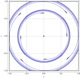
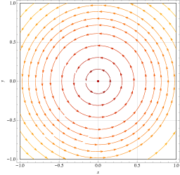
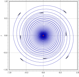
Figure 1. Comparison of different RM schemes for bilinear games $\Phi(x,y)=xy$, $x,y\in\mathbb{R}$. From left to right: (a) gradient descent/ascent; (b) the mean dynamics (MD); (c) extra-gradient.

Lemma 2.

Let $Z_{n+1}=Z_{n}+\gamma_{n}[V(Z_{n})+W_{n}]$ be an RM scheme where $W_{n}=U_{n}+b_{n}$ as in (5). Then its alternating version, defined as

$$X_{n+1} =X_{n}+\gamma_{n} [V_{x}(X_{n},Y_{n})+W_{x,n}],$$ (alt-RM)

$$Y_{n+1} =Y_{n}+\gamma_{n} [V_{y}(X_{n+1},Y_{n})+W_{y,n}],$$

is also an RM scheme: $Z_{n+1}=Z_{n}+\gamma_{n}[V(Z_{n})+U_{n}+b^{\prime}_{n}]$ where

$$b^{\prime}_{n}=b_{n}+\begin{bmatrix}0\\ V_{y}(X_{n+1},Y_{n})-V_{y}(X_{n},Y_{n})\end{bmatrix}.$$

Remark 3.2.

One can easily generalize Lemma 2 to the “$(k_{1},k_{2})$-RM schemes” where one performs $k_{1}$ updates for $x$ and then $k_{2}$ updates for $y$ (here $k_{1},k_{2}\in\mathbb{N}$ are arbitrary but fixed). The resulting scheme will still be an RM scheme. In particular, our framework captures the popular $(k_{1},k_{2})=(1,5)$ variant of (SGDA) used in the seminal works of Goodfellow et al [32] and Arjovsky et al [3]. In view of Lemmas 1–2, Remark 3.2, and a simple calculation (see (B.18)), all of our results on first-order methods (e.g., Algorithms 1–4) apply also to their averaging/alternating and the more general $(k_{1},k_{2})$ versions.

4. Convergence analysis

4.1. Overview: Continuous vs. discrete time

The key in providing a unified treatment of all algorithms in Section 3 is the reduction of (RM) to the mean dynamics

$$\dot{z}(t)=V(z(t)).$$ (MD)

To see why (MD) can capture the limiting behavior of a vast family of RM schemes beyond GDA, let us illustrate the high-level intuition on the deterministic version of Algorithm 3 ($U_{n}=0$).

Since $\Phi$ and $V$ are assumed to be Lipschitz (say with constants $M$ and $L$), we see that the bias term in Algorithm 3 satisfies

$$\lVert b_{n}\rVert=\lVert V(Z_{n}^{+})-V(Z_{n})\rVert\leq L\lVert Z_{n}^{+}-Z_{n}\rVert=\gamma_{n}L\lVert V(Z_{n})\rVert\leq\gamma_{n}LM=\operatorname{\mathcal{O}}(\gamma_{n}).$$ (7)

As a result, we can rewrite Algorithm 3 as

$$\frac{Z_{n+1}-Z_{n}}{\gamma_{n}}=V(Z_{n})+\mathcal{O}(\gamma_{n}).$$ (8)

If $\gamma_{n}\searrow 0$, we should then expect (8) to converge to (MD). More generally, if the error term $W_{n}$ in (RM) is sufficiently well-behaved, we should expect the iterates of (RM) and the solutions of (MD) to eventually come together.

Connecting (RM) to (MD) has proved very fruitful when the latter comprises a gradient system, i.e., $V=-\nabla f$ for some (possibly non-convex) $f\colon\mathcal{Z}\to\mathbb{R}$: Modulo mild assumptions, the systems (RM) and (MD) are known to both converge to the critical set of $f$ [55, 48, 10, 50, 11].

On the other hand, bona fide min-max problems are considerably more involved. The most widely known illustration is given by the bilinear objective $\Phi(x,y)=xy$: in this case (see Fig. 1), the trajectories (MD) comprise periodic orbits of perfect circles centered at the origin (the unique critical point of $\Phi$). However, the behavior of different RM schemes can vary wildly, even in the absence of noise ($\sigma=0$): trajectories of (SGDA) spiral outwards, each converging to an initialization-dependent periodic orbit; instead, (SEG) trajectories spiral inwards, eventually converging to the solution $z^{\ast}=(0,0)$.

This particular difference between gradient and extra-gradient schemes has been well-documented in the literature [21, 30, 59]. More pertinent to our theory, it also raises several key questions:

1. What is the precise link between RM methods and the mean dynamics (MD)?

2. When does (MD) yield accurate predictions for the long-run behavior of an RM method?

Below, we devote Sections 4.2–4.3 to the first question, and Section 4.4 to the second.

4.2. Connecting (RM) to (MD)

We begin by introducing a measure of “closeness” between the iterates of (RM) and the solution orbits of (MD). To do so, let $\tau_{n}=\sum\nolimits_{k=1}^{n}\gamma_{k}$ denote the “effective time” that has elapsed at the $n$-th iteration of (RM), and define the continuous-time interpolation $Z(t)$ of $Z_{n}$ as

$$Z(t)=Z_{n}+\frac{t-\tau_{n}}{\tau_{n+1}-\tau_{n}}(Z_{n+1}-Z_{n})$$ (9)

for all $t\in[\tau_{n},\tau_{n+1}]$, $n\geq 1$. To compare $Z(t)$ to the solution orbits of (MD), we will further consider the flow $\Theta\colon\mathbb{R}_{+}\times\mathcal{Z}\to\mathcal{Z}$ of (MD), which is simply the orbit of (MD) at time $t\in\mathbb{R}_{+}$ with an initial condition $z(0)=z\in\mathcal{Z}$. We then have the following notion of “asymptotic closeness”:

Definition 1.

$Z(t)$ is an asymptotic pseudotrajectory (APT) of (MD) if, for all $T>0$, we have:

$$\textstyle\lim_{t\to\infty}\sup_{0\leq h\leq T}\lVert Z(t+h)-\Theta_{h}(Z(t))\rVert=0.$$ (10)

This comparison criterion is due to Benaïm and Hirsch [9] and it plays a central role in our analysis. In words, it simply posits that $Z(t)$ eventually tracks the flow of (MD) with arbitrary accuracy over windows of arbitrary length; as a result, if $Z_{n}$ is an asymptotic pseudotrajectory (APT) of (MD), it is reasonable to expect its behavior to be closely correlated to that of (MD).

Our first result below makes this link precise. Consider an RM scheme which satisfies

$$\textstyle B_{n}\to 0\;\;\text{{(}a.s.{)}}\quad\text{and}\quad\sum_{n=1}^{\infty}\operatorname{\mathbb{E}}[\gamma_{n}B_{n}]<\infty$$ (A1)

$$\textstyle\sum\nolimits_{n=1}^{\infty}\operatorname{\mathbb{E}}[\gamma_{n}^{2}(1+B_{n}^{2}+\sigma_{n}^{2})]<\infty\hskip 10.00002pt$$ (A2)

We then have:

Theorem 1.

Suppose that Eqs. A1–A2 hold. Then $Z_{n}$ is an APT of (MD) w.p.$1$.

4.3. Applications and examples

Of course, applying Theorem 1 to a specific algorithm (e.g., as in Section 3) would first require verifying Eqs. A1–A2. However, even though the noise $\operatorname{\mathsf{U}}(z;\omega)$ in (SFO) is assumed zero-mean and finite-variance, this does not imply that the error term $W_{n}=U_{n}+b_{n}$ in Algorithms 2–5 enjoys the same guarantees. For example, the RM representation of Algorithms 2–4 has non-zero bias, while Algorithm 5 has non-zero bias and unbounded variance (the latter behaving as $\operatorname{\mathcal{O}}(1/\delta_{n}^{2})$ with $\delta_{n}\to 0$).

In the following proposition we prove that Algorithms 1–5 generate asymptotic pseudotrajectories of (MD) for the typical range of hyperparameters used to ensure almost sure convergence of stochastic first-order methods.

Proposition 1.

Let $Z_{n}$ be a sequence generated by any of the Algorithms 1–5. Assume further that:

1. For first-order methods (Algorithms 1–4), the algorithm is run with SFO feedback satisfying (3) and a step-size $\gamma_{n}$ such that $A/n\leq\gamma_{n}\leq B/\sqrt{n(\log n)^{1+\varepsilon}}$ for some $A,B,\varepsilon>0$.

2. For zeroth-order methods (Algorithm 5), the algorithm is run with parameters $\gamma_{n}$ and $\delta_{n}$ such that $\lim_{n}(\gamma_{n}+\delta_{n})=0$, $\sum_{n}\gamma_{n}=\infty$, and $\sum_{n}\gamma_{n}^{2}/\delta_{n}^{2}<\infty$ (e.g., $\gamma_{n}=1/n$, $\delta_{n}=1/n^{1/3}$).

Then $Z_{n}$ is almost surely an APT of (MD).

4.4. The limit sets of RM schemes

The APT results in Sections 4.2–4.3 can be heuristically interpreted as: “RM schemes eventually behave as some orbits of (MD).” We now further ask: What are the candidate limit orbits of (MD) for RM schemes?

To shed some light on the question, let us recall that, in non-convex minimization problems, SGD enjoys the following properties:

1. SGD converges to the function’s set of critical points [55, 11].

2. SGD avoids unstable critical points [70, 29, 60].

This leads to the following “law of the excluded middle”: generically, the only solution candidates left for SGD are stable critical points, i.e., the local minimizers of the problem’s minimization objective.

In the remaining of this section, we will assimilate Items (I) and (II) in the context of RM schemes applied to (SP).

4.4.1. The long-run limit of RM schemes

We first focus on generalizing Item (I) for min-max optimization. To proceed, recall first that critical points alone cannot capture the broad spectrum of algorithmic behaviors when (MD) is not a gradient system: already in Fig. 1 we see a critical point surrounded by spurious periodic orbits. In addition, in dynamical systems many other spurious convergence phenomena are known, such as homoclinic loops, limit cycles, or chaos. To account for this considerably richer landscape, we will need some definitions from the theory of dynamical systems.

Definition 2 (7).

Let $\mathcal{S}$ be a nonempty compact subset of $\mathcal{Z}$. Then:

1. $\mathcal{S}$ is invariant if $\Theta_{t}(\mathcal{S})=\mathcal{S}$ for all $t\in\mathbb{R}$.

2. $\mathcal{S}$ is attracting if it is invariant and there exists a compact neighborhood $\mathcal{K}$ of $\mathcal{S}$ such that $\lim_{t\to\infty}\operatorname{dist}(\Theta_{t}(z),\mathcal{S})=0$ uniformly in $z\in\mathcal{K}$.

3. $\mathcal{S}$ is internally chain-transitive (ICT) if it is invariant and $\Theta|_{\mathcal{S}}$ admits no proper attractors in $\mathcal{S}$.

Remark.

Equivalently, ICT sets can be viewed as “minimal connected periodic orbits up to arbitrarily small numerical errors”, cf. Benaïm [7, Prop. 5.3]. The definition above is more convenient to work with because it provides the key insights in Section 4.4.3 below.

Our next result shows that, with probability $1$, all limit points of (RM) lie in these “approximate periodic orbits”:

Theorem 2.

If Eqs. A1–A2 hold, then $Z_{n}$ converges almost surely to an ICT set of $\Phi$.

Corollary 1.

Let $Z_{n}$ be a sequence generated by any of the Algorithms 1–5 with parameters as in Proposition 1. Then $Z_{n}$ converges almost surely to an ICT set of $\Phi$.

4.4.2. Avoidance of unstable points and sets

Our next result provides an avoidance result for RM schemes in min-max optimization. In analogy with function minimization problems, we will focus on unstable invariant sets of (MD), i.e., invariant sets that admit a nontrivial unstable manifold (for an in-depth discussion and precise definition, see 81 and Section C.1).

In generic minimization problems, these are precisely the sets of strict saddle points of the function being minimized. However, since general min-max problems do not comprise a gradient system, (MD) could exhibit a plethora of unstable sets, not containing any stationary points of $\Phi$ (e.g., periodic orbits, heteroclinic networks, etc.). On account of the above, our result below is stated in terms of invariant sets – and not only points. For convenience, we will assume that $V$ is $C^{2}$ and $\gamma_{n}$ is as in Proposition 1.

Theorem 3.

Let $\mathcal{K}$ be an unstable invariant set of (MD) (which trivially includes unstable periodic orbits and unstable critical points). Assume further that the noise in (RM) satisfies: (i1pt) $\sup_{n}\lVert U_{n}\rVert<\infty$w.p.$1$; and (ii1pt) $\inf_{z:\lVert z\rVert=1}\operatorname{\mathbb{E}}\left[\langle U_{n},z\rangle_{+}\nonscript\,|\nonscript\,\mathopen{}\mathcal{F}_{n}\right]>0$. Then $Z_{n}$ generated by any of the Algorithms 1–4 satisfies

$$\textstyle\operatorname{\mathbb{P}}\left({\lim_{n\to\infty}\operatorname{dist}(Z_{n},\mathcal{K})=0}\right)=0.$$

Remark 4.1.

We note that Items (i1pt) and (ii1pt) above are standard in the literature for avoidance results of SGD [70, 7, 60], and are significantly lighter than other “isotropic noise” assumptions that are common in the literature [29]. Specifically, even though Item (ii1pt) looks somewhat obscure, it only posits that the noise is not degeneratively equal to zero along certain directions in space; for a more detailed discussion, see Section C.1. We also stress that neither of these assumptions is required for the rest of our paper.

4.4.3. When do RM schemes behave the same?

So far, we have successfully generalized Items (I) and (II) to the context of (SP) as follows:

1. RM schemes always converge to ICT sets, and

2. RM schemes always avoid invariant sets.

Nonetheless, Items I and II still fail to explain the distinct behaviors of RM schemes in bilinear objectives: Why does SGDA converge only to periodic orbits, while deterministic stochastic extra-gradient (SEG) only to critical points? Or, more generally, Are different RM schemes more likely to exhibit different convergence topologies – e.g., cycles vs. critical points – in generic min-max problems?

Our next result takes a closer look at attracting ICT sets and provides a generically negative answer to this question. To set the stage, suppose we want to apply Item I to the bilinear objective $\Phi(x,y)=xy$. Stricto sensu, Item I does not apply in this case since $\Phi$ is not Lipschitz. However, Fig. 1(b) shows (and we rigorously prove in Section C.2) that any tuple $(x,y)\in\mathbb{R}^{2}$ belongs to an ICT set of $\Phi$, so Theorem 2 holds trivially. This in turn implies that the only attractor for $\Phi$ is trivially the whole space $\mathbb{R}^{2}$, since Definition 2-2 is never satisfied for any $\mathcal{S}\subsetneq\mathbb{R}^{2}$.

Importantly, the celebrated Kupka-Smale theorem [47, 82] asserts that systems with degenerate periodic orbits (such as bilinear games) occur “almost never” in the Baire category sense. More precisely, an arbitrarily small perturbation can fundamentally destroy the topological properties of their ICT sets and give rise to proper, non-trivial attractors; cf. Example 5.1. In contrast, systems with nontrivial attractors are known to be robust under perturbations [81], and our final result in the section shows that it is precisely the existence of nontrivial attractors that makes the discrepancy of RM schemes disappear, at least locally.

Theorem 4.

Let $\mathcal{S}$ be an attractor of (MD) and fix some confidence level $\alpha>0$. If $\gamma_{n}$ is small enough and Eqs. A1–A2 hold, there exists a neighborhood $\mathcal{U}$ of $\mathcal{S}$, independent of $\alpha$, such that $\operatorname{\mathbb{P}}(\text{$Z_{n}$ converges to $\mathcal{S}$})\geq 1-\alpha$ if $Z_{1}\in\mathcal{U}$.

Corollary 2.

Let $Z_{n}$ be a sequence generated by any of the Algorithms 1–5 with sufficiently small $\gamma_{n}$ satisfying the conditions of Proposition 1. If $Z_{1}\in\mathcal{U}$, then $\operatorname{\mathbb{P}}(\text{$Z_{n}$ converges to $\mathcal{S}$})\geq 1-\alpha$.

In short, Theorem 4 asserts that any non-degenerate ICT set dictates the local convergence of all RM schemes under the general Eqs. A1–A2.

On a positive note, since the Hartman-Grobman Theorem [78] implies that all critical points of $\Phi$ with $\Re\{\lambda(JV(z^{\ast}))\}<0$ for all engenvalues $\lambda$ are attractors of (MD), Theorem 4 immediately yields:

Corollary 3.

Let $z^{\ast}$ be a critical point of $\Phi$ such that $\Re\{\lambda(JV(z^{\ast}))\}<0$ for all engenvalues of $JV(z^{\ast})$. Then all RM schemes satisfying Eqs. A1–A2 locally converge to $z^{\ast}$ with high probability.

Corollary 3 generalizes the local convergence of deterministic SGDA and SEG studied by Daskalakis and Panageas [20]. It also extends [37, Theorem 5] from (OG/PEG) to all generalized RM schemes.

On the flip side, however, Theorem 4 also bears an undesirable consequence: it implies that many RM schemes designed to improve SGDA (e.g., Algorithms 2–4) may in fact be trapped by spurious ICT sets in exactly the same way as SGDA. Thus, even though many of these algorithms have been motivated by their appealing properties in bilinear games, it is not clear whether they offer any significant advantages beyond the convex-concave case. We examine this issue in detail in the next section.

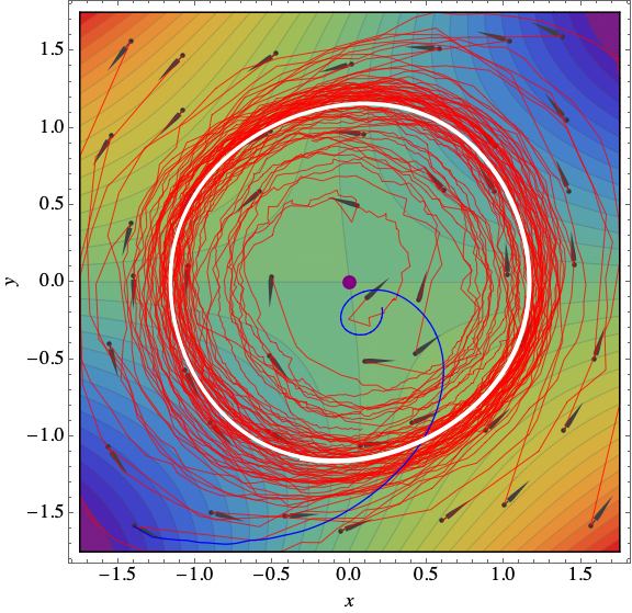
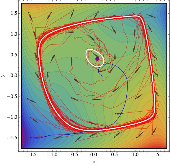
Figure 2. Spurious limits of min-max optimization algorithms. From left to right: (a) (SEG) for (11) with $\varepsilon=0.01$; (b) “forsaken solutions” of (SEG); The red curves present trajectories with different initialization; non-critical ICT sets are depicted in white; the blue curves represent an time-averaged sample orbit.

5. Spurious attractors: Illustrations and examples

In this last section, we provide a range of simple examples that exhibit spurious attractors –  i.e., attractors that consist entirely of non-critical points. For illustration purposes, we focus on the simple case $\mathcal{X}=\mathcal{Y}=\mathbb{R}$ with polynomial objectives. In doing this, our goal is to highlight a number of issues that can arise in min-max optimization problems; whether limit cycles of this type occur in actual large-scale experiments – e.g., in GANs – is an open research question [52].

$\blacktriangledown$ Example 5.1 (Almost bilinear $\not\approx$ bilinear, instability $\not\approx$ escape).

Consider an arbitrarily small perturbation of a bilinear game:

$$\Phi(x,y)=xy+\varepsilon\phi(y),$$ (11)

where $\varepsilon>0$ and $\phi(y)=\frac{1}{2}y^{2}-\frac{1}{4}y^{4}$. There is an unstable critical point at the origin; further, Lemma D.1 asserts, for small $\varepsilon$, the existence of an attracting ICT set $\mathcal{S}$ in a neighborhood of the circle $\{z:\lVert z\rVert^{2}=4/3\}$. By Corollary 2, any RM scheme of Section 3 thus gets trapped by $\mathcal{S}$; see Fig. 2(a) for an illustration for (SEG).

This example brings two issues of existing studies to light. First, it shows that “almost bilinear games” can still trap many methods for solving exact bilinear games. Second, in contrast to minimization problems, the region around an unstable critical point can in fact be fully stable. Thus, one has to be careful when interpreting algorithms that “locally avoid unstable critical points”, since they might be incapable of escaping their neighborhoods. $\blacktriangle$

$\blacktriangledown$ Example 5.2 (“Forsaken” $\min\max$ solutions).

Suppose we apply Algorithms 1–5 to the objective

$$\Phi(x,y)=x(y-0.45)+\phi(x)-\phi(y)$$ (12)

where $\phi(z)=\frac{1}{4}z^{2}-\frac{1}{2}z^{4}+\frac{1}{6}z^{6}$. This problem has a desirable $(x^{\ast},y^{\ast})\simeq(0.08,0.4)$. However, as we show in Section D.2, there exist two spurious limit cycles that do not contain any critical point of $\Phi$. Worse, the limit cycle closer to the solution is unstable and repels any trajectory that comes close to the solution; see Fig. 2(b) for an illustration for (SEG). As a result, the “shielded” solution is highly unlikely to be discovered by existing algorithms, even though it is perfectly stable. $\blacktriangle$

We conclude the paper by further examining several important settings that are not covered by our theory:

1. Instead of the “moving average” in Lemma 1, one can take the ergodic average ($Z^{\prime}_{n}=\frac{1}{n}\sum\nolimits_{k=1}^{n}Z_{k}$) as is customary in convex-concave problems [66, 42]. We plot one such trajectory in Fig. 2 (the blue curves). Evidently, we see that ergodic average can force the algorithms to halt at non-critical points, and this convergence is by no means min-max optimal.

2. Many recent works attempt to address the cycling issues of min-max algorithms via incorporating second-order oracles. For completeness, we also study a range of popular second-order methods in Section D.3. Our analysis shows that these algorithms suffer similar symptoms as first-order schemes in our examples, cf. Figs. 4–5.

3. In addition to the diminishing step-size policies studied here, another common strategy in practice is to simply set $\gamma_{n}$ to a constant step-size. While our analysis does not cover this setting, there exist several techniques in stochastic approximation to boost from our “almost surely” statements for $\gamma_{n}\searrow 0$ to concentration or high-probability results when $\gamma_{n}\equiv\gamma$ is small [49, 50, 12].

   For completeness, in Section D.4 we examine various constant step-size RM schemes applied to (11) and (12). The outcome coincides with our intuition that these schemes should concentrate around the spurious attracting ICT sets, and hence exhibit similar behaviors as RM schemes with $\gamma_{n}\searrow 0$; see Fig. 6.

4. Adaptive methods such as Adam [46] are ubiquitous in GAN training. We study such methods in Section D.5: our results show tha they fail solve the simple objectives (11) and (12). Moreover, some methods even show a potentially detrimental tendency of converging to max-min points, the exact opposite of desirable solutions; see Fig. 7.

In closing, we should clarify that these illustrations are not meant to suggest that the algorithms and practical tweaks discussed above are always doomed, or that they comprise the principal cause of failure in GAN training. However, we do believe that they constitute an important cautionary tale to the effect that, in min-max problems, convergence does not imply optimality – or even stationarity.

Appendix A Stabilization of RM schemes

Our aim in this appendix will be to prove the stability of generalized RM schemes, namely that asymptotic pseudotrajectories generated by (RM) are bounded with probability $1$. The key ingredient in our analysis is the weak asymptotic coercivity (WAC) condition (2), which, as we discussed in the main body of our paper, is a relaxation of the standard coercivity requirement

$$\lim_{\lVert z\rVert\to\infty}\frac{\langle V(z),z\rangle}{\lVert z\rVert}=-\infty.$$ (A.1)

The hypothesis (A.1) is a mainstay in the analysis of monotone operators and variational inequalities [6, 24, 73]. Roughly speaking, it states that the “radial component”

$$V_{r}(z)=\frac{\langle V(z),z\rangle}{\lVert z\rVert}$$ (A.2)

of $V(z)$ grows to $-\infty$ as $\lVert z\rVert\to\infty$. In other words, any vector field that satisfies (A.1) has an inward-pointing component that grows infinitely large for large $\lVert z\rVert$.

In view of the above, the coercivity assumption (A.1) suggests that any process that takes successive steps along $V(z)$ will be subject to an “inwards drift” towards regions with smaller norm, and this drift will be more and more pronounced the farther one moves away from the origin. On that account, (A.1) is a natural candidate for showing that RM processes based on $V$ never escape to infinity. On the other hand, vector fields that do not have a strong radial component – such as the bilinear game field $V(x,y)=(-y,x)$ which has $V_{r}(x,y)=0$ – are not covered by (A.1). In this regard, the WAC condition (2) provides an important relaxation of (A.1), because it only posits that the radial component of $V(z)$ is asymptotically non-positive – or, more simply, that $V(z)$ does not have a persistent outward-pointing component.

Before proving the stability of generalized RM schemes under (2), we provide below a series of important examples that satisfy the WAC condition (2):

1. $V$ satisfies (A.1). Indeed, in this case, for all $M>0$, there exists some $R\equiv R(M)$ such that

   $$\frac{\langle V(z),z\rangle}{R}\leq\frac{\langle V(z),z\rangle}{\lVert z\rVert}\leq-M<0$$ (A.3)

   whenever $\lVert z\rVert\geq R$, i.e., (2) holds

2. $\Phi$ is convex-concave and it admits a critical point. By shifting the problem’s frame of reference if necessary, we can assume without loss of generality that $z^{\ast}=0$ is a critical point of $\Phi$. Then, with $\Phi$ assumed convex-concave, we readily get $\langle V(z),z\rangle\leq\langle V(z^{\ast}),z-z^{\ast}\rangle=0$, i.e., (2) holds

The first item above justifies the terminology “weak asymptotic coercivity”; for a geometric illustration, see Fig. 3 below.

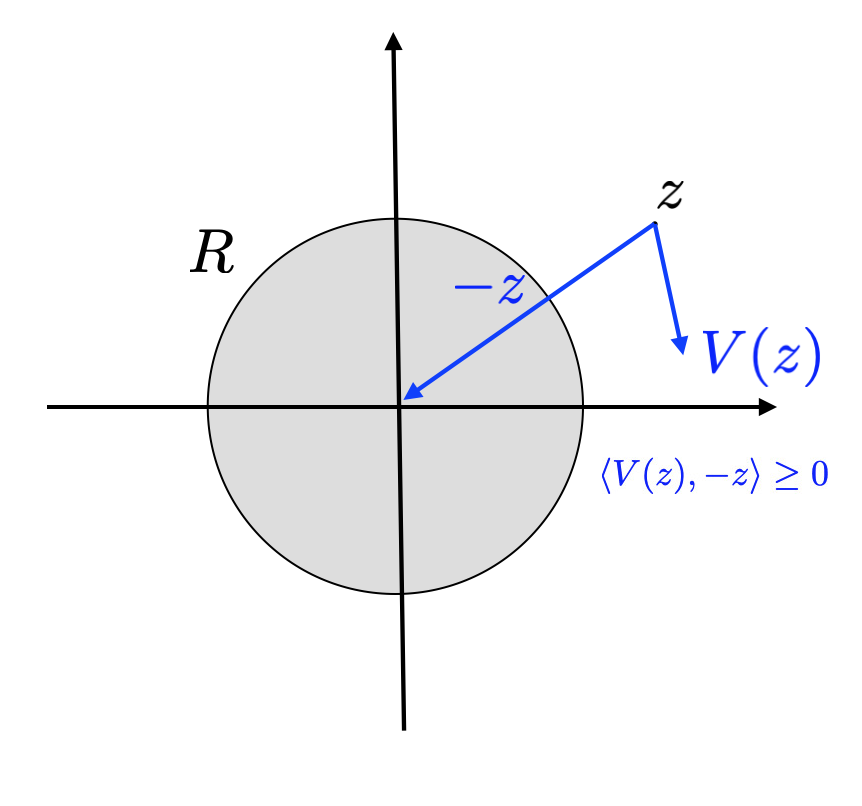
Figure 3. Schematic illustration of the weak asymptotic coercivity condition Eq. 2.

We now proceed to establish our main stability result for generalized RM schemes under the WAC condition (2):

Proposition A.1.

Suppose that $V$ satisfies Eq. 2. Then, under Eqs. A1–A2, the sequence $Z_{n}$ generated by (RM) is bounded (a.s.).

Proof of Proposition A.1.

Our proof hinges on the introduction of a suitable “energy function” for (MD). To define it, recall that that $\langle V(z),-z\rangle\geq 0$ whenever $\lVert z\rVert\geq R$. Then, with a fair amount of hindsight, fix some $\lambda>0$ and let

$$E(z)=\begin{cases}0&\quad\text{if $\lVert z\rVert\leq R$},\\ (\lVert z\rVert-R)^{2}/2&\quad\text{if $R\leq\lVert z\rVert\leq(1+\lambda)R$},\\ \lambda R\lVert z\rVert-\lambda(1+\lambda/2)R^{2}&\quad\text{if $(1+\lambda)R\leq\lVert z\rVert$}.\end{cases}$$ (A.4)

By a direct calculation, we can verify the following:

1. $E$ is continuously differentiable and its gradient is given by $\nabla E(z)=\phi(\lVert z\rVert/R)\,z$ where $\phi(u)=0$ if $u\leq 1$, $\phi(u)=1-1/u$ if $1\leq u\leq 1+\lambda$, and $\phi(u)=\lambda/u$ if $1+\lambda\leq u$.

2. $E$ is negatively correlated to $V$, i.e., $\langle V(z),-\nabla E(z)\rangle\geq 0$ for all $z\in\mathcal{Z}$.

3. $E$ is $1$-smooth, i.e., $E(z^{\prime})\leq E(z)+\langle\nabla E(z),z^{\prime}-z\rangle+(1/2)\lVert z^{\prime}-z\rVert^{2}$ for all $z,z^{\prime}\in\mathcal{Z}$.

Then, letting $E_{n}=E(Z_{n})$ and $\phi_{n}=\phi(\lVert Z_{n}\rVert/R)$, we get

$$E_{n+1}=E(Z_{n}-\gamma_{n}V_{n}) \leq E(Z_{n})-\gamma_{n}\langle\nabla E(Z_{n}),V_{n}\rangle+\frac{\gamma_{n}^{2}}{2}\lVert V_{n}\rVert^{2}$$

$$\leq E_{n}-\gamma_{n}\phi_{n}\langle U_{n}+b_{n},Z_{n}\rangle+\frac{3\gamma_{n}^{2}}{2}\big{[}\lVert V(Z_{n})\rVert^{2}+\lVert U_{n}\rVert^{2}+\lVert b_{n}\rVert^{2}\big{]},$$ (A.5)

where the second line follows from the properties of $E$, the definition (4) of $V_{n}$, and the Cauchy-Schwarz inequality. Hence, conditioning on $\mathcal{F}_{n}$ and taking expectations, we obtain:

$$\operatorname{\mathbb{E}}[E_{n+1}\nonscript\,|\nonscript\,\mathopen{}\mathcal{F}_{n}]\leq E_{n}+\gamma_{n}\phi_{n}\lVert Z_{n}\rVert B_{n}+\tfrac{3}{2}\gamma_{n}^{2}\big{[}M^{2}+B_{n}^{2}+\sigma_{n}^{2}\big{]},$$ (A.6)

where we made a second use of the Cauchy-Schwarz inequality in the term involving $B_{n}$ and $M$ is the Lipschitz constant of $\Phi$.

To proceed, let $\varepsilon_{n}=\gamma_{n}\phi_{n}\lVert Z_{n}\rVert B_{n}+(3/2)\gamma_{n}^{2}[M^{2}+B_{n}^{2}+\sigma_{n}^{2}]$ denote the “residual” term in (A.6), and consider the auxiliary process $\tilde{E}_{n}=E_{n+1}+\sum_{k=n+1}^{\infty}\varepsilon_{k}$. By (A.6), we have $\operatorname{\mathbb{E}}[\tilde{E}_{n}\nonscript\,|\nonscript\,\mathopen{}\mathcal{F}_{n}]\leq E_{n}+\sum_{k=n}^{\infty}\varepsilon_{n}=\tilde{E}_{n-1}$, i.e., $\tilde{E}_{n}$ is a supermartingale relative to $\mathcal{F}_{n}$. By the definition of $\phi$, we further have $\phi(u)\leq\lambda/u$, so $\phi_{n}\lVert Z_{n}\rVert\leq\lambda R$ for all $n$. We thus get

$$\sum_{n=1}^{\infty}\varepsilon_{n}\leq\lambda R\sum_{n=1}^{\infty}\gamma_{n}B_{n}+\frac{3}{2}\sum_{n=1}^{\infty}\gamma_{n}^{2}(M^{2}+B_{n}^{2}+\sigma_{n}^{2})$$ (A.7)

and hence, by Eqs. A1 and A2, we conclude that $\operatorname{\mathbb{E}}[\sum_{n}\varepsilon_{n}]<\infty$. This shows that $\operatorname{\mathbb{E}}[\tilde{E}_{n}]\leq\operatorname{\mathbb{E}}[\tilde{E}_{1}]<\infty$, i.e., $\tilde{E}_{n}$ is uniformly bounded in $L^{1}$. Hence, by Doob’s submartingale convergence theorem [35, Theorem 2.5], it follows that $\tilde{E}_{n}$ converges with probability $1$ to some finite random limit $\tilde{E}_{\infty}$. In turn, since $\sum_{n}\varepsilon_{n}<\infty$, this implies that $E_{n}=\tilde{E}_{n-1}-\sum_{k=n}^{\infty}\varepsilon_{n}$ also converges to some (random) finite limit (a.s.). From this we deduce that $\limsup_{n}\lVert Z_{n}\rVert<\infty$, as claimed. ∎

Appendix B Proof of Theorems 1 and 1

In this appendix, we discuss how the algorithms in Section 3 fit within the general stochastic approximation framework of Section 4.2. Specifically, we prove the general conditions of Theorems 1 and 1 which guarantee that Algorithms 1–5 generate asymptotic pseudotrajectories of the mean dynamics (MD).

B.1. Generalities and preliminaries

Before doing so, we will require some background material on asymptotic pseudotrajectories. Following Benaïm and Hirsch [9] and Benaïm [7], we first recall the definition of the “effective time” $\tau_{n}=\sum_{k=1}^{n}\gamma_{k}$ as the time that has elapsed at the $n$-th iteration of the discrete-time process $Z_{n}$; recall also the definition (9) of the continuous-time interpolation $Z(t)$ of $Z_{n}$ as

$$Z(t)=Z_{n}+\frac{t-\tau_{n}}{\tau_{n+1}-\tau_{n}}(Z_{n+1}-Z_{n})$$ (9)

We will further require the “continuous-to-discrete” correspondence

$$M(t)=\sup\{n\geq 1:t\geq\tau_{n}\}$$ (B.1)

which measures the number of iterations required for the effective time $\tau_{n}$ of the process to reach the timestamp $t$; for future use, we also define the quantity

$$M_{n}\equiv M_{n}(T)=M(\tau_{n}+T).$$ (B.2)

Finally, given an arbitrary sequence $A_{n}$, we will denote its piecewise constant interpolation as

$$\overline{A}(t)=A_{n}\quad\text{for all $t\in[\tau_{n},\tau_{n+1}]$, $n\geq 1$.}$$ (B.3)

Using this notation, the (affinely) interpolated process $Z(t)$ can be expressed in integral form as

$$Z(t)=Z(0)+\int_{0}^{t}[V(\overline{Z}(s))+\overline{W}(s)]\>ds$$ (B.4)

where $W_{n}$ denotes the generalized error term of (RM).

With all this in hand, Benaïm [7, Prop. 4.1] provides the following general condition for $Z(t)$ to be an APT of the mean dynamics (10):

Proposition B.1.

Suppose that $Z(t)$ is bounded and satisfies the general condition

$$\lim_{t\to\infty}\Delta(t;T)=0\quad\text{for all $T>0$},$$ (B.5)

where

$$\textstyle\Delta(t;T)=\sup_{0\leq h\leq T}\left\lVert\int_{t}^{t+h}\overline{W}(s)\>ds\right\rVert.$$ (B.6)

Then, $Z(t)$ is an APT of (MD).

B.2. Proof of Theorem 1

Our proof of Theorem 1 revolves around the direct verification of the requirement (B.5) of Proposition B.1 via the use of maximal inequalities and martingale limit theory. For convenience, we restate the theorem below in full:

See 1

Proof.

Since we have shown that $Z_{n}$ remains bounded in Proposition A.1, it suffices to verify (B.5).

Our proof relies on the Burkholder–Davis–Gundy (BDG) inequality [14, 35] which bounds the maximal value of a martingale $S_{n}$ via its quadratic variation as

$$c_{2}\operatorname{\mathbb{E}}\left[\sum_{k=1}^{n}(S_{k}-S_{k-1})^{2}\right]\leq\operatorname{\mathbb{E}}\left[\max_{k=1,\dotsc,n}\lvert S_{k}\rvert^{2}\right]\leq C_{2}\operatorname{\mathbb{E}}\left[\sum_{k=1}^{n}(S_{k}-S_{k-1})^{2}\right],$$ (BDG)

where $c_{2},C_{2}>0$ are universal constants. As such, applying (BDG) to the martingale $S_{m}=\sum_{k=n}^{m}\gamma_{k}U_{k}$ (after an appropriate shift of the starting time), we get

$$\operatorname{\mathbb{E}}\left[\sup_{n\leq m\leq M_{n}}\left\lVert\sum_{k=n}^{m}\gamma_{k}U_{k}\right\rVert^{2}\right] \leq C_{2}\operatorname{\mathbb{E}}\left[\sum_{k=n}^{M_{n}}\gamma_{k}^{2}\lVert U_{k}\rVert^{2}\right]$$

$$=C_{2}\sum_{k=n}^{M_{n}}\gamma_{k}^{2}\sigma_{k}^{2}=C_{2}\int_{\tau_{n}}^{\tau_{n}+T}\overline{\gamma}^{2}(s)\overline{\sigma}^{2}(s)\>ds,$$ (B.7)

where $M_{n}=M_{n}(T)=M(\tau_{n}+T)$ is defined as in (B.2). Now, mimicking (B.6), let

$$\Delta_{0}(t;T)=\sup_{0\leq h\leq T}\left\lVert\int_{t}^{t+h}\overline{U}(s)\>ds\right\rVert.$$ (B.8)

so our previous bound shows that

$$\operatorname{\mathbb{E}}[\Delta_{0}(t;T)^{2}] \leq C_{2}\int_{t}^{t+T}\overline{\gamma}^{2}(s)\overline{\sigma}^{2}(s)\>ds.$$ (B.9)

We will proceed to show that $\lim_{t\to\infty}\Delta_{0}(t;T)=0$ for all $T>0$ by considering the sequence of intervals $[kT,(k+1)T]$ and using the Borel-Cantelli lemma in order to show that $\Delta_{0}(kT;T)\to 0$ as $k\to\infty$. Indeed, we have

$$\sum_{k=1}^{\infty}\operatorname{\mathbb{E}}[\Delta_{0}(kT;T)^{2}] \leq C_{2}\int_{0}^{\infty}\overline{\gamma}^{2}(s)\overline{\sigma}^{2}(s)\>ds=C_{2}\sum_{n=1}^{\infty}\gamma_{n}^{2}\sigma_{n}^{2}<\infty$$ (B.10)

with the last step following from Eq. A2. Then, if we consider the event $\mathcal{E}_{k}(\varepsilon)=\{\Delta_{0}(kT;T)>\varepsilon\}$, Chebysev’s inequality gives

$$\sum_{k=1}^{\infty}\operatorname{\mathbb{P}}(\mathcal{E}_{k}(\varepsilon))\leq\frac{\sum_{k=1}^{\infty}\operatorname{\mathbb{E}}[\Delta_{0}(kT;T)^{2}]}{\varepsilon^{2}}<\infty,$$ (B.11)

and hence, by the Borel-Cantelli lemma, we get

$$\operatorname{\mathbb{P}}\left(\limsup_{k\to\infty}\mathcal{E}_{k}(\varepsilon)\right)=0.$$ (B.12)

This shows that, with probability $1$, we have $\Delta_{0}(kT;T)\leq\varepsilon$ for all but a finite number of $k$; put differently, the event $\mathcal{E}(\varepsilon)=\{\text{$\Delta_{0}(kT;T)$ occurs infinitely often}\}=\operatorname*{\bigcap}_{n=1}^{\infty}\operatorname*{\bigcup}_{k=n}^{\infty}\mathcal{E}_{k}(\varepsilon)$ has $\operatorname{\mathbb{P}}(\mathcal{E}(\varepsilon))=0$. Therefore, as a union of probability zero events, we have

$$\operatorname{\mathbb{P}}\left(\liminf_{k\to\infty}\Delta_{0}(kT;T)>0\right)=\operatorname{\mathbb{P}}\left(\operatorname*{\bigcup}_{n=1}^{\infty}\mathcal{E}(1/n)\right)\leq\sum_{n=1}^{\infty}\operatorname{\mathbb{P}}(\mathcal{E}(1/n))=0,$$ (B.13)

i.e., $\Delta_{0}(kT;T)\to 0$ with probability $1$.

Thus, going back to the requirements of Proposition B.1, we get

$$\Delta(kT;T) =\sup_{0\leq h\leq T}\left\lVert\int_{kT}^{kT+h}\overline{W}(t)\>dt\right\rVert=\sup_{0\leq h\leq T}\left\lVert\int_{kT}^{kT+h}[\overline{U}(t)+\overline{b}(t)]\>dt\right\rVert$$

$$\leq\Delta_{0}(kT;T)+\sup_{0\leq h\leq T}\int_{kT}^{kT+h}\overline{B}(t)\>dt.$$

$$\leq\Delta_{0}(kT;T)+T\max_{0\leq h\leq T}\overline{B}(kT+h).$$ (B.14)

Given that $\lim_{k\to\infty}B_{k}=0$, the above shows that $\Delta(kT;T)\to 0$ as $k\to\infty$. Moreover, for all $t\in[kT,(k+1)T]$, we have $\Delta(t;T)\leq 2\Delta(kT;T)+\Delta((k+1)T;T)$ so $\Delta(t;T)\to 0$ with probability $1$. With $T>0$ arbitrary, we conclude that (B.5) holds with probability $1$, so our claim follows from Proposition B.1. ∎

B.3. Proof of Proposition 1

We are now in a position to prove that the generalized RM schemes presented in Section 3 comprise asymptotic pseudotrajectories of the mean dynamics (MD). For convenience, we state the relevant result below:

See 1

Proof.

We first note that $\sum_{n}\gamma_{n}^{2}<\infty$ by our choice of step-sizes. Thus, in order to prove that $\operatorname{\mathbb{E}}[\sum_{n}\gamma_{n}B_{n}]<\infty$, $\operatorname{\mathbb{E}}[\sum_{n}\gamma_{n}^{2}B_{n}^{2}]<\infty$, and $\operatorname{\mathbb{E}}[\sum_{n}\gamma_{n}^{2}\sigma_{n}^{2}]<\infty$, it suffices to show $\operatorname{\mathbb{E}}[B_{n}]=\operatorname{\mathbb{E}}[\lVert b_{n}\rVert]=\operatorname{\mathcal{O}}(\gamma_{n})$ and $\operatorname{\mathbb{E}}[\sigma_{n}^{2}]\leq\sigma^{2}$ for some constant $\sigma$.

We next proceed method-by-method:

Algorithm 1: SGDA.

For (SGDA), we have $W_{n}=U_{n}=\operatorname{\mathsf{U}}(Z_{n};\omega_{n})$ and $b_{n}=0$, so Eq. A1 is satisfied automatically (since $B_{n}=0$). Our claim then follows from the stated assumptions for (SFO).

Algorithm 2: PPM.

For (PPM), we have $U_{n}=0$ and

$$\lVert b_{n}\rVert =\lVert V(Z_{n})-V(Z_{n+1})\rVert$$

$$\leq L\lVert Z_{n}-Z_{n+1}\rVert$$

$$=\gamma_{n}L\lVert V(Z_{n})\rVert$$

$$\leq\gamma_{n}LM=\operatorname{\mathcal{O}}(\gamma_{n}).$$

where $L$ and $M$ are the Lipschitz constant of $V$ and $\Phi$, respectively.

Algorithm 3: SEG.

For (SEG), we have $U_{n}=\operatorname{\mathsf{U}}(Z_{n}^{+};\omega_{n}^{+})$ and $b_{n}=V(Z_{n}^{+})-V(Z_{n})$ so that $\operatorname{\mathbb{E}}[\sigma_{n}^{2}]\leq\sigma^{2}$ by (SFO). To verify Eq. A1, by the definition of (SEG), we have

$$\lVert b_{n}\rVert=\lVert V(Z_{n}^{+})-V(Z_{n})\rVert \leq L\lVert Z_{n}^{+}-Z_{n}\rVert$$

$$=\gamma_{n}\lVert\operatorname{\mathsf{V}}(Z_{n};\omega_{n})\rVert=\gamma_{n}L\lVert V(Z_{n})+\operatorname{\mathsf{U}}(Z_{n};\omega_{n})\rVert$$

$$\leq\gamma_{n}L\lVert V(Z_{n})\rVert+\gamma_{n}L\lVert\operatorname{\mathsf{U}}(Z_{n};\omega_{n})\rVert.$$ (B.15)

Since $\Phi$ is assumed to be Lipschitz and $\operatorname{\mathsf{U}}(Z_{n};\omega_{n})$ finite variance, taking the expectation on both sides of the above shows $\operatorname{\mathbb{E}}[B_{n}]=\operatorname{\mathcal{O}}(\gamma_{n})$. It remains to verify that $\lim_{n\to\infty}B_{n}=0$ with probability 1. Now, by Chebyshev’s inequality and (SFO), we have

$$\operatorname{\mathbb{P}}\left({\lVert\operatorname{\mathsf{U}}(Z_{n};\omega_{n})\rVert\geq\sqrt{n\log^{1+\frac{\epsilon}{2}}n}}\right)\leq\frac{\sigma^{2}}{n\log^{1+\frac{\epsilon}{2}}n}$$ (B.16)

where $\varepsilon$ is the same as in our choice of step-size in Proposition 1. In turn, this implies that

$$\sum_{n=2}^{\infty}\operatorname{\mathbb{P}}\left({\lVert\operatorname{\mathsf{U}}(Z_{n};\omega_{n})\rVert\geq\sqrt{n\log^{1+\frac{\epsilon}{2}}n}}\right)<\infty$$

so, by the Borel-Cantelli lemma, we have $\lVert\operatorname{\mathsf{U}}(Z_{n};\omega_{n})\rVert=\operatorname{\mathcal{O}}\left(\sqrt{n\log^{1+\frac{\epsilon}{2}}n}\right)$ with probability $1$. Hence, by our assumptions for the method’s step-size, we get

$$\gamma_{n}\lVert\operatorname{\mathsf{U}}(Z_{n};\omega_{n})\rVert=\operatorname{\mathcal{O}}\left(\frac{\sqrt{n\log^{1+\frac{\epsilon}{2}}n}}{\sqrt{n\log^{1+\varepsilon}n}}\right)=\operatorname{\mathcal{O}}\left(\frac{1}{\log^{\frac{\varepsilon}{4}}n}\right)$$ (B.17)

so that, in view of (B.3), $B_{n}\to 0$ with probability $1$.

Algorithm 4: OG.

For (OG/PEG), we have $U_{n}=\operatorname{\mathsf{U}}(Z_{n};\omega_{n}^{+})$ and $b_{n}=V(Z_{n}^{+})-V(Z_{n})$, so $\operatorname{\mathbb{E}}[\sigma_{n}^{2}]=\sigma^{2}$ again holds by (SFO). The bias term can then be bounded exactly as in the case of Algorithm 3.

Algorithms 1–4: Alternating RM schemes (alt-RM).

We now show that the alternating version of Algorithms 1–4 still constitute an APT of (MD).

By Lemma 2, we know that the alternating version of an RM scheme is another RM scheme with the same noise and new bias satisfying:

$$\lVert b^{\prime}_{n}\rVert \leq\lVert b_{n}\rVert+\lVert V_{y}(X_{n+1},Y_{n})-V_{y}(X_{n},Y_{n})\rVert$$

$$\leq\lVert b_{n}\rVert+L\lVert X_{n+1}-X_{n}\rVert$$

$$\leq\lVert b_{n}\rVert+\gamma_{n}L\left(\lVert V(Z_{n})\rVert+\lVert b_{n}\rVert+\lVert U_{n}\rVert\right)$$ (B.18)

by the definition of an RM scheme. Since $\gamma_{n}L\lVert b_{n}\rVert=o\left(\lVert b_{n}\rVert\right)$, the rest is the same as Algorithm 3.

We also note that (B.18) can be applied recursively to show that the bias term $b_{n}^{(k_{1},k_{2})}$ of any $(k_{1},k_{2})$ version of RM schemes satisfy

$$\lVert b_{n}^{(k_{1},k_{2})}\rVert\leq(k_{1}+k_{2}-1)\Big{(}\lVert b_{n}\rVert+\gamma_{n}L\left(\lVert V(Z_{n})\rVert+\lVert b_{n}\rVert+\lVert U_{n}\rVert\right)\Big{)},$$ (B.19)

thus enjoying the same properties as the vanilla alternating $(1,1)$-RM schemes in view of (B.18).

Algorithm 5: SPSA.

Because of the algorithm’s different oracle structure (zeroth- vs. first-order feedback), the analysis of (5) is different. We begin with the algorithm’s bias term, given here by

$$b_{n} =\operatorname{\mathbb{E}}[V_{n}\nonscript\,|\nonscript\,\mathopen{}\mathcal{F}_{n}]-V(Z_{n})$$ (B.20)

with

$$V_{n}=\pm(d/\delta_{n})\,\Phi(Z_{n}+\delta_{n}\omega_{n})\,\omega_{n}$$ (B.21)

denoting the method’s one-shot SPSA estimator. To bound it, let

$$v_{i,n}=\operatorname{\mathbb{E}}[V_{i,n}\nonscript\,|\nonscript\,\mathopen{}\mathcal{F}_{n}]$$ (B.22)

denote the $i$-th component of $V_{n}\in\mathbb{R}^{d}$ after having averaged out the choice of the random seed $\omega_{n}$ (which, by default, is not $\mathcal{F}_{n}$-measurable). We then have

$$v_{i,n} =\pm\frac{d}{\delta_{n}}\cdot\frac{1}{2d}\big{[}\Phi(Z_{n}+\delta_{n}e_{i})-\Phi(Z_{n}-\delta_{n}e_{i})\big{]}$$ (B.23)

where, as per our discussion in Section 3, the “$\pm$” sign is equal to $-1$ if $e_{i}\in\mathcal{E}_{\mathcal{X}}$ and $+1$ if $e_{i}\in\mathcal{E}_{\mathcal{Y}}$. Then, by the mean value theorem, there exists some $\tilde{E}_{n}$ in the line segment $\big{[}Z_{n}-\delta_{n}e_{i},Z_{n}+\delta_{n}e_{i}\big{]}$ such that

$$v_{i,n}=\pm\partial_{i}\Phi(\tilde{E}_{n})=V_{i,n}(\tilde{E}_{n}).$$ (B.24)

Since $V$ is Lipschitz continuous, it follows that

$$\lvert v_{i,n}-V_{i,n}(Z_{n})\rvert =\big{\lvert}V_{i,n}(\tilde{E}_{n})-V_{i,n}(Z_{n})\big{\rvert}\leq L\lVert\tilde{E}_{n}-Z_{n}\rVert=\operatorname{\mathcal{O}}(\delta_{n})$$ (B.25)

since $\tilde{E}_{n}\in\big{[}Z_{n}-\delta_{n}e_{i},Z_{n}+\delta_{n}e_{i}\big{]}$. Finally, for the oracle’s variance, we have $\lVert V_{n}\rVert^{2}=\operatorname{\mathcal{O}}(1/\delta_{n}^{2})$ by construction so, under the stated assumptions for $\gamma_{n}$ and $\delta_{n}$, Eq. A2 is satisfied and our claim follows from Theorem 1. ∎

Appendix C Convergence analysis: Proof of Theorems 3–4

With all this preliminary work in hand, we are finally in a position to prove Theorems 3–4.

The heavy lifting for Theorem 2 is already provided by the fact that, under the requirements of Theorem 1 and/or Proposition 1, $Z_{n}$ is an APT of the mean dynamics (MD), so it inherits its limit structure. Theorems 3 and 4 on the other hand require a completely different set of techniques and involve a much finer analysis of the process in hand.

C.1. Avoidance of unstable periodic orbits

While the proof of Theorem 3 is highly technical, the high-level intuition for its conclusion is crystal clear: Assume that we are given an unstable critical point $z^{*}$. Then, by the stable manifold theorem [81], the set of all initializations such that the flow of (MD) converges to $z^{*}$ is of measure 0 in $\mathcal{Z}$. Consequently, if the noise process $\{U_{n}\}$ is such that it has “non-negligible” magnitude in the unstable directions near $z^{*}$, then it is plausible that the RM scheme should escape $z^{*}$ along these directions. Item (ii1pt) in Theorem 3 quantifies exactly the magnitude of noise for which we can formalize this heuristic argument.

Throughout this section we assume that we are given:

• A $(d-m)$-dimensional embedded submanifold $\mathcal{S}\subset\mathbb{R}^{d}$ where $1\leq m\leq d$ and $d-m$ is to be understood as the dimension of the unstable manifold.

• A nonempty compact set $\mathcal{K}\subset\mathcal{S}$ invariant under $\Theta\coloneqq\{\Theta_{t}:t\in\mathbb{R}_{+}\}$.

• We also assume that $\mathcal{S}$ is $C^{2}$ is locally invariant: there exists a neighborhood $\mathcal{U}$ of $\mathcal{K}$ in $\mathbb{R}^{d}$ and a positive time $t_{0}$ such that

  $$\Theta_{t}(\mathcal{U}\cap\mathcal{S})\subset\mathcal{S}$$ (C.1)

  for all $\lvert t\rvert\leq t_{0}$.

We further assume that for every point $z\in\mathcal{K}$, we have

$$\mathbb{R}^{d}=T_{z}\mathcal{S}\oplus\mathcal{E}^{u}_{{z}}$$ (C.2)

where

1. $z\to\mathcal{E}^{u}_{{z}}$ is a continuous map from $\mathcal{K}$ into the Grassmanian manifold $G({m},d)$ of $m$ planes in $\mathbb{R}^{d}$.

2. $\operatorname{D}\Theta_{t}(z)\mathcal{E}^{u}_{{z}}=\mathcal{E}^{u}_{{\Theta_{t}(z)}}$ for all $t\in\mathbb{R},z\in\mathcal{E}^{u}_{{z}}$.

3. There exist $\lambda,C>0$ such that for all $z\in\mathcal{K},w\in\mathcal{E}^{u}_{{z}}$ and $t\geq 0$

   $$\lVert\operatorname{D}\Theta_{t}(z)w\rVert\geq Ce^{\lambda t}\lVert w\rVert.$$ (C.3)

We call any $\mathcal{K}$ satisfying the above an unstable invariant set. As a simple illustration we show:

Lemma C.1.

If $z^{\ast}$ is a critical point of $\Phi$ with any eigenvalue $\lambda$ of $JV(z^{\ast})$ such that $\Re\{\lambda(JV(z^{\ast}))\}>0$. Then $z^{\ast}$ verifies all the assumptions of an unstable invariant set.

As a corollary, $Z_{n}$ generated by any of the Algorithms 1–4 in Theorem 3 avoids $z^{\ast}$ almost surely.

Proof.

All the requirements for an unstable invariant set are readily verified by the Stable Manifold Theorem [78]. The lemma follows by noting the the dimension for the unstable manifold is greater than or equal to 1; see [78, Chap 5]. ∎

A further justification of these technical assumptions is the following: Suppose $\mathcal{K}$ is a periodic orbit. We then say that $\mathcal{K}$ is (linearly) unstable if 1 is a Floquet multiplier of $\mathcal{K}$ and some multipliers have modulus strictly greater than 1 [84]. If the vector field $V$ is assumed to be $C^{2}$, then a classical result in dynamical systems (see e.g., [81]) states that $\mathcal{K}$ verifies all the above assumptions.

We now proceed to the proof of Theorem 3. For ease of reading we reformulate its statements in the following more convenient form:

Theorem 2.

Let $\mathcal{K}$ be an unstable invariant set of $V$. Assume that

1. There exists $K>0$ such that $\lVert U_{n}\rVert\leq K$ for all $n$.

2. $\gamma_{n}$ is as in Proposition 1.

3. There exists a neighborhood $\mathcal{U}(\mathcal{K})$ of $\mathcal{K}$ and $b>0$ such that for all unit vector $v\in\mathbb{R}^{d}$

   $$\operatorname{\mathbb{E}}[\langle U_{n+1},v\rangle^{+}|\mathcal{F}_{n}]\geq b\operatorname{\mathds{1}}_{\{Z_{n}\in\mathcal{U}(\mathcal{K})\}}.$$

4. The vector field $V$ is $C^{2}$.

Then $Z_{n}$ generated by any of the Algorithms 1–4 satisfies

$$\operatorname{\mathbb{P}}\left({\lim_{n\to\infty}\operatorname{dist}(Z_{n},\mathcal{K})=0}\right)=0.$$

proof of Theorem 3.

We first note that, for our choice of $\gamma_{n}$,

$$\lim_{n\to\infty}\frac{\gamma_{n}}{\sqrt{\sum\nolimits_{k=n}^{\infty}\gamma_{k}^{2}}}=0$$ (C.4)

so $\gamma_{n}=o\left(\sqrt{\sum\nolimits_{k=n}^{\infty}\gamma_{k}^{2}}\right)$. This fact will be used in the proof when we invoke Lemma C.3 below with $\varepsilon_{n}=\operatorname{\mathcal{O}}(\gamma_{n})$ and $\alpha_{n}=\sum\nolimits_{k=n}^{\infty}\gamma_{k}^{2}$ therein.

Helper lemmas.

We will need some technical lemmas. The first one is a deep result by Benaïm and Hirsch [8], which asserts the existence of a local Lyapunov function near the unstable periodic orbits.

For a right-differentiable function $\eta:\mathbb{R}^{d}\to\mathbb{R}$ we define its right derivative $\operatorname{D}\eta$ applied to a vector $h\in\mathbb{R}^{d}$ by

$$\operatorname{D}\eta(z)h=\lim_{t\to 0^{+}}\frac{\eta(z+th)-\eta(z)}{t}.$$ (C.5)

If $\eta$ is differentiable, then (C.5) is simply $\langle\operatorname{\nabla}\eta(z),h\rangle$.

Lemma C.2.

There exists a compact neighborhood $\mathcal{U}(\mathcal{K})$ of $\mathcal{K}$, positive numbers $l,\beta>0$, and a map $\eta:\mathcal{U}(\mathcal{K})\to\mathbb{R}$ such that:

1. $\eta$ is $C^{2}$ on $\ \mathcal{U}(\mathcal{K})\setminus\mathcal{S}$.

2. For all $z\in\mathcal{U}(\mathcal{K})\cap\mathcal{S}$, $\eta$ admits a right derivative $\operatorname{D}\eta(z):\mathbb{R}^{d}\to\mathbb{R}^{d}$ which is Lipschitz, convex and positively homogeneous.

3. There exists $k>0$ and a neighborhood $\mathcal{W}\subset\mathbb{R}^{d}$ of $0$ such that for all $z\in\mathcal{U}(\mathcal{K})$ and $v\in\mathcal{W}$

   $$\eta(z+v)\geq\eta(z)+{\operatorname{D}\eta(z)}{v}-k\lVert v\rVert^{2}.$$ (C.6)

4. There exists $c_{1}>0$ such that for all $z\in\mathcal{U}(\mathcal{K})\setminus\mathcal{S}$

   $$\lVert\operatorname{\nabla}\eta(z)\rVert\geq c_{1}$$ (C.7)

   and for all $z\in\mathcal{U}(\mathcal{K})\cap\mathcal{S}$ and $v\in\mathbb{R}^{d}$

   $$\langle\operatorname{D}\eta(z),v\rangle\geq c_{1}\lVert v-\operatorname{D}\operatorname{\Pi}(z)v\rVert.$$ (C.8)

5. For all $z\in\mathcal{U}(\gamma)\cap\mathcal{S}$, $u\in T_{z}\mathcal{S}$ and $v\in\mathbb{R}^{d}$

   $${\operatorname{D}\eta(z)}{(u+v)}={\operatorname{D}\eta(z)}{v}.$$ (C.9)

6. For all $z\in\mathcal{U}(\mathcal{K})$ we have

   $${\operatorname{D}\eta(z)}{V(z)}\geq\beta\eta(z).$$ (C.10)

The second lemma we need is a probabilistic estimate from [71].

Lemma C.3.

Let $S_{n}$ be a nonnegative stochastic process, $S_{n}=S_{0}+\sum\nolimits_{k=1}^{n}X_{k}$ where $X_{n}$ is $\mathcal{F}_{n}$-measurable.  Let $\alpha_{n}\coloneqq\sum\nolimits_{k=n}^{\infty}\gamma_{k}^{2}$.

Assume there exist a sequence $0\leq\varepsilon_{n}=o(\sqrt{\alpha_{n}})$, constants $a_{1},a_{2}>0$ and an integer $N_{0}$ such that for all $n\geq N_{0}$,

1. $\lvert X_{n}\rvert=o(\sqrt{\alpha_{n}})$.

2. $\operatorname{\mathds{1}}_{\{S_{n}>\varepsilon_{n}\}}\operatorname{\mathbb{E}}[X_{n+1}|\mathcal{F}_{n}]\geq 0$.

3. $\operatorname{\mathbb{E}}[S^{2}_{n+1}-S^{2}_{n}|\mathcal{F}_{n}]\geq a_{1}\gamma^{2}_{n}$.

4. $\operatorname{\mathbb{E}}[X^{2}_{n+1}|\mathcal{F}_{n}]\leq a_{2}\gamma^{2}_{n}.$

Then $\operatorname{\mathbb{P}}(\lim_{n\to\infty}\nolimits S_{n}=0)=0.$

Armed with Lemmas C.2 and C.3 we are now ready to prove Theorem 3.

Let $N\in\mathbb{N}$. Assume $z_{N}\in\mathcal{U}(\mathcal{K})$ where $\mathcal{U}(\mathcal{K})$ is the neighborhood given by Lemma C.2. Define $T$ as

$$T\coloneqq\inf\{k\geq N:Z_{n}\notin\mathcal{U}(\mathcal{K})\}.$$ (C.11)

Evidently, $T$ is a stopping time adaptive to $\mathcal{F}_{n}$. Thus, proving Theorem 3 amounts to showing $\operatorname{\mathbb{P}}(T<\infty)=1$. Without loss of generality we may assume $N=0$.

Define two sequences of random variables $\{X_{n}\}_{n\geq 2}$ and $\{S_{n}\}$ as

$$X_{n+1}= (\eta(Z_{n+1})-\eta(Z_{n}))\operatorname{\mathds{1}}_{\{n\leq T\}}+\gamma_{n}\operatorname{\mathds{1}}_{\{n>T\}},$$ (C.12a)

$$S_{0}=\eta(Z_{0}),\quad S_{n}=S_{0}+\sum_{k=2}^{n}X_{i}.$$ (C.12b)

Note that $S_{n}\geq 0$ (a.s.) for every $n$. Our proof will revolve around verifying Lemma C.3Items 1–4.

Verifying Lemma C.3Items 1 and 4 .

By Lipschitz continuity of $\eta$ we know that

$$\lVert\eta(Z_{n})-\eta(Z_{n+1})\rVert \leq L^{\prime}\lVert Z_{n}-Z_{n+1}\rVert$$

$$=\gamma_{n}\lVert V(Z_{n})+U_{n}+b_{n}\rVert$$ (C.13)

where $L^{\prime}$ is the Lipschitz constant of $\eta$. We have seen in the proof of Proposition 1 that $\lVert b_{n}\rVert=\operatorname{\mathcal{O}}\left(\gamma_{n}(\lVert V(Z_{n})\rVert+\lVert U_{n}\rVert)\right)$. By Proposition A.1 and Item (i1pt) in Theorem 3, we then have $\lvert X_{n+1}\rvert=\operatorname{\mathcal{O}}({\gamma_{n}})=o(\sqrt{\alpha_{n}})$ which implies both Lemma C.3Items 1 and 4.

Verifying Lemma C.3Item 2 .

Let $k^{\prime}=k\lVert V\rVert+K$ where $k$ is given by Lemma C.2Item iii and $\lVert V\rVert\coloneqq\sup\{V(z):z\in\mathcal{U}(\mathcal{K})\}$ and $K$ is the uniform bound of $U_{n}$. If $n\leq T$, using Lemma C.2Items ii, iii, v and vi we have

$$\eta(Z_{n+1})-\eta(Z_{n}) \geq\gamma_{n}\operatorname{D}\eta(Z_{n})\left(U_{n}+b_{n}+V(Z_{n})\right)-k\gamma_{n}^{2}\left(\lVert V\rVert+\lVert U_{n}\rVert+\lVert b_{n}\rVert\right)^{2}$$

$$\geq\gamma_{n}\beta\eta(Z_{n})+\gamma_{n}\operatorname{D}\eta(Z_{n})U_{n}+\gamma_{n}\operatorname{D}\eta(Z_{n})b_{n}-2k^{\prime}\gamma_{n}^{2}-2k\gamma_{n}^{2}\lVert b_{n}\rVert^{2}.$$ (C.14)

By the same calculation leading up to (B.3), Item (i1pt) in Theorem 3, and the Lipschitz continuity of $\Phi$, there exists a constant $c^{\prime}>0$ such that the bias sequence for Algorithms 1–4 can be bounded as $-\lVert b_{n}\rVert\geq-c^{\prime}\gamma_{n}$ (a.s.). Combining this with the Lipschitz continuity of $\eta$, we can merge the last three terms in (C.1) as

$$\eta(Z_{n+1})-\eta(Z_{n}) \geq\gamma_{n}\beta\eta(Z_{n})+\gamma_{n}\operatorname{D}\eta(Z_{n})U_{n}-2k^{\prime\prime}\gamma_{n}^{2}$$ (C.15)

for some constant $k^{\prime\prime}>0$. Thus

$$\operatorname{\mathds{1}}_{\left\{n\leq T\right\}}\operatorname{\mathbb{E}}[X_{n+1}|\mathcal{F}_{n}]\geq\operatorname{\mathds{1}}_{\left\{n\leq T\right\}}\left[\gamma_{n}\beta\eta(Z_{n})-2k^{\prime\prime}\gamma_{n}^{2}+\gamma_{n}\operatorname{\mathbb{E}}[\operatorname{D}\eta(Z_{n})U_{n}|\mathcal{F}_{n}]\right].$$ (C.16)

By Lemma C.2Item ii again, we have

$$\operatorname{\mathbb{E}}[\operatorname{D}\eta(Z_{n})U_{n}|\mathcal{F}_{n}]\geq\operatorname{D}\eta(Z_{n})\operatorname{\mathbb{E}}[U_{n}|\mathcal{F}_{n}]=0$$ (C.17)

since we have assumed noise to be zero mean. Combining (C.16) and (C.17), we then get

$$\operatorname{\mathds{1}}_{\left\{n\leq T\right\}}\operatorname{\mathbb{E}}[X_{n+1}|\mathcal{F}_{n}]\geq\operatorname{\mathds{1}}_{\left\{n\leq T\right\}}\left[\gamma_{n}\beta\eta(Z_{n})-2k^{\prime\prime}\gamma_{n}^{2}\right].$$ (C.18)

If $n>T$, $X_{n+1}=\gamma_{n}$ so trivially

$$\operatorname{\mathds{1}}_{\left\{n\leq T\right\}}\operatorname{\mathbb{E}}[X_{n+1}|\mathcal{F}_{n}]\geq 0.$$ (C.19)

Combining (C.18) with (C.19), we see that Lemma C.3Item 2 is satisfied with $\varepsilon_{n}=\frac{k^{\prime\prime}}{\beta}\gamma_{n}$.

Verifying Lemma C.3Item 3 .

We begin by observing that

$$\operatorname{\mathbb{E}}[S_{n+1}^{2}-S_{n}^{2}|\mathcal{F}_{n}]=\operatorname{\mathbb{E}}[X_{n+1}^{2}|\mathcal{F}_{n}]+2S_{n}\operatorname{\mathbb{E}}[X_{n+1}|\mathcal{F}_{n}].$$ (C.20)

If $S_{n}\geq\varepsilon_{n}$, then the right-hand side of (C.20) is non-negative by Lemma C.3Item 2 that we just verified above. If $S_{n}<\varepsilon_{n}$, (C.18) with (C.19) imply that $S_{n}\operatorname{\mathbb{E}}[X_{n+1}|\mathcal{F}_{n}]\geq-\varepsilon_{n}k^{\prime\prime}\gamma_{n}^{2}=-\operatorname{\mathcal{O}}(\gamma_{n}^{3})$. In other words, (C.20) can be rewritten as

$$\operatorname{\mathbb{E}}[S_{n+1}^{2}-S_{n}^{2}|\mathcal{F}_{n}]\geq\operatorname{\mathbb{E}}[X_{n+1}^{2}|\mathcal{F}_{n}]-\operatorname{\mathcal{O}}(\gamma_{n}^{3}).$$ (C.21)

Below, we shall prove that $\operatorname{\mathbb{E}}[X_{n+1}^{2}|\mathcal{F}_{n}]\geq b_{1}\gamma_{n}^{2}$ for some $b_{1}>0$ and $n$ large enough. Combining this with (C.21) proves Lemma C.3Item 3.

From (C.15), we deduce

$$\operatorname{\mathds{1}}_{\left\{n\leq T\right\}}\left[\operatorname{\mathbb{E}}[X^{+}_{n+1}|\mathcal{F}_{n}]-\left(\gamma_{n}\operatorname{\mathbb{E}}[(\operatorname{D}\eta(Z_{n})U_{n})^{+}|\mathcal{F}_{n}]-k^{\prime\prime}\gamma_{n}^{2}\right)\right]\geq 0.$$ (C.22)

Invoking Lemma C.2Item iv and Item (ii1pt) in Theorem 3, we see that

$$\operatorname{\mathds{1}}_{\{n\leq T\}\cap\{Z_{n}\notin\mathcal{S}\}}\Big{(}\operatorname{\mathbb{E}}[(\operatorname{D}\eta(Z_{n})U_{n})^{+}|\mathcal{F}_{n}]-c_{1}b\Big{)}\geq 0$$ (C.23)

If $Z_{n}\in\mathcal{S}$, we can choose a unit vector $v_{n}\in\ker(I-\operatorname{D}\operatorname{\Pi}(Z_{n}))^{\perp}$ where $\operatorname{\Pi}$ denotes the projection operator onto $\mathcal{S}$. By the definition of $v_{n}$, we have $\langle U_{n},v_{n}\rangle=\langle U_{n}-\operatorname{D}\operatorname{\Pi}(Z_{n})U_{n},v_{n}\rangle$. Let $\mathcal{H}=\{n\leq T\}\cap\{Z_{n}\notin\mathcal{S}\}.$ By Lemma C.2Item iv, Cauchy-Schwartz, and Item (ii1pt) of Theorem 3 we get

$$\operatorname{\mathds{1}}_{\mathcal{H}}\operatorname{\mathbb{E}}[(\operatorname{D}\eta(Z_{n})U_{n})^{+}|\mathcal{F}_{n}] \geq c_{1}\operatorname{\mathds{1}}_{\mathcal{H}}\operatorname{\mathbb{E}}[\lVert U_{n}-\operatorname{D}\operatorname{\Pi}(Z_{n})U_{n}\rVert|\mathcal{F}_{n}]$$

$$\geq c_{1}\operatorname{\mathds{1}}_{\mathcal{H}}\operatorname{\mathbb{E}}[\langle U_{n}-\operatorname{D}\operatorname{\Pi}(Z_{n})U_{n},v_{n}\rangle^{+}|\mathcal{F}_{n}]$$

$$=c_{1}\operatorname{\mathds{1}}_{\mathcal{H}}\operatorname{\mathbb{E}}[\langle U_{n},v_{n}\rangle^{+}|\mathcal{F}_{n}]$$

$$\geq c_{1}b\operatorname{\mathds{1}}_{\mathcal{H}}.$$ (C.24)

Combining Eqs. C.19, C.22, C.23 and C.24 then gives

$$\operatorname{\mathbb{E}}[X^{+}_{n+1}|\mathcal{F}_{n}]\geq\gamma_{n}c_{1}b-k^{\prime\prime}\gamma_{n}^{2}.$$ (C.25)

On the other hand, we always have $\operatorname{\mathbb{E}}[X^{2}_{n+1}|\mathcal{F}_{n}]\geq\operatorname{\mathbb{E}}[X^{+}_{n+1}|\mathcal{F}_{n}]$ by Jensen. It then follows that $\operatorname{\mathbb{E}}[X^{2}_{n+1}|\mathcal{F}_{n}]\geq b_{1}\gamma_{n}^{2}$ for some $b_{1}>0$ and large enough $n$ as desired.

Closing the gap.

We have now verified Lemma C.3Items 1–4. Thus, Lemma C.3 concludes that

$$\operatorname{\mathbb{P}}(\lim\nolimits_{n\to\infty}S_{n}=0)=0.$$ (C.26)

We will use (C.26) to show that $T<\infty$ (a.s.).

Suppose $T=\infty$. Then $X_{n+1}=\eta(Z_{n+1})-\eta(Z_{n})$ and $S_{n}=\eta(Z_{n})$ by (C.12a)-(C.12b), and $\{Z_{n}\}$ remains in $\mathcal{U}(\mathcal{K})$ by definition of the stopping time $T$. Theorem 2 then asserts the the limit set $L(\{Z_{n}\})$ of $\{Z_{n}\}$ is a nonempty compact invariant subset of $\mathcal{U}(\mathcal{K})$, so that for all $z^{\prime}\in L(\{Z_{n}\})$ and $t\in\mathbb{R}$, $\Theta_{t}(z^{\prime})\in\mathcal{U}(\mathcal{K}).$ But then Lemma C.2Item iv implies that $\eta(\Theta_{t}(z^{\prime}))\geq e^{\beta t}\eta(z^{\prime})$ for all $t>0$, forcing $\eta(z^{\prime})$ to be zero. In other words, we have $L(\{Z_{n}\})\subset\mathcal{S}$, which implies $S_{n}=\eta(Z_{n})\to 0$ . By (C.26), this event occurs with probability 0, thus showing that $T$ is finite almost surely. ∎

C.2. Convergence to ICTs

We now prove Theorem 2, which we restate below for convenience:

See 2

Proof.

By Theorem 1, $Z_{n}$ generates APT of the mean dynamics (MD). Now, let $\mathcal{L}=\operatorname*{\bigcap}_{t\geq 0}\operatorname{cl}(Z(t,\infty))$ be the limit set of $Z(t)$, i.e., the set of limit points of convergent sequences $Z(t_{n})$ with $\lim_{n}t_{n}=\infty$. Our claim then follows by the limit set theorem of Benaïm and Hirsch [9, Theorem 8.2]. ∎

As we discussed in the main part of our paper, the ICT sets of $\Phi$ may exhibit a wide variety of structural properties (limit cycles, heteroclinic networks, etc.). As a complement to this, we show below that, in gradient systems ($V=-\nabla f$ for some $f\colon\mathcal{Z}\to\mathbb{R}$), ICT sets can only be compoments of equilibria. Specifically, building on a general result by Benaïm [7], we have:

Proposition C.1.

Suppose that $V(z)=-\nabla f(z)$ for some $C^{d}$-smooth potential function $f\colon\mathcal{Z}\to\mathbb{R}$ with a compact critical set $\operatorname{crit}(f)=\{z^{\ast}:\nabla f(z^{\ast})=0\}$. Then, every ICT set $\mathcal{S}$ of (MD) is contained in $\operatorname{crit}(f)$; moreover, $f$ is constant on $\mathcal{S}$. In particular, any ICT set of (MD) consists solely of critical points of $f$.

Proof.

Under the stated conditions, the critical set $\mathcal{Z}^{\ast}\coloneqq\operatorname{crit}(f)$ of $f$ coincides with the set of rest points of (MD). Moreover, by Sard’s theorem [51], $f(\mathcal{Z}^{\ast})$ has zero Lebesgue measure and hence empty interior. Our claim then follows from Proposition 6.4 of Benaïm [7]. ∎

As another elementary illustration in addition to the gradient systems, one can show that for bilinear games $\Phi(x,y)=xy$, the ICT sets the whole space $\mathbb{R}^{2}$.  This can be easily seen by considering the widely known Hamiltonian function $H(x,y)=x^{2}+y^{2}$, which satisfies $\dot{H}=0$ provided $(x,y)$ follows (MD). An immediate consequence of this fact is that any point on $\mathbb{R}^{2}$ lies in some ICT set of (MD), which further implies that there is no bounded attracting region, i.e., attractors.

C.3. Convergence to attractors

We now proceed with the analysis of RM schemes in the presence of an attractor; the relevant result is Theorem 4:

See 4

Because of the generality of our assumptions, the proof of Theorem 4 requires a range of completely different arguments and techniques. We illustrate the main steps of our technical trajectory below:

1. The first crucial component of our proof is to establish an energy function for (RM) in a neighborhood of $\mathcal{S}$. To do this, we rely on Conley’s decomposition theorem (the so-called “fundamental theorem of dynamical systems”) which states that the mean dynamics (MD) are “gradient-like” in a neighborhood of an attractor, i.e., they admit a (local) Lyapunov function.

2. Because of the noise in (RM), the evolution of $E$ along the trajectories of (RM) could present signifcant jumps: in particular, a single “bad” realization of the noise could carry $Z_{n}$ out of the basin of attraction of $\mathcal{S}$, possibly never to return. A major difficulty here is that the driving vector field $V$ is not assumed bounded, so it is not straightforward to establish proper control over the error terms of (RM). However, we show that, with high probability (and, in particular, with probability at least $1-\alpha$), the aggregation of these errors remains controllably small; this is the most technically challenging part of our argument and it unfolds in a series of lemmas below.

3. Conditioning on the above, we will show that, with probability at least $1-\alpha$, the value of the trajectory’s energy cannot grow more than a token threshold $\varepsilon$; as a result, if (RM) is initialized close to $\mathcal{S}$, it will remain in a neighborhood thereof for all $n$ (again, with probability at least $1-\alpha$).

4. Thanks to this “stochastic Lyapunov stability” result, we can regain control of the variance of the process and use martingale limit and maximal inequality arguments to show that $Z_{n}$ converges to $\mathcal{S}$.

In the rest of this section, we make this roadmap precise via a series of technical lemmas and intermediate results.

A local energy function for (RM).

We begin by providing a suitable energy function for (MD). Indeed, since $\mathcal{S}$ is an attractor of (MD), there exists a compact neighborhood $\mathcal{K}$ of $\mathcal{S}$, called the fundamental neighborhood of $\mathcal{S}$, with the property that $\operatorname{dist}(\Theta_{t}(z){t}{z},\mathcal{S})\to 0$ as $t\to\infty$ uniformly in $z\in\mathcal{K}$. Since all trajectories of (MD) that start in $\mathcal{K}$ converge to $\mathcal{S}$, there are no other non-trivial invariant sets in $\mathcal{K}$ except $\mathcal{S}$. Hence, with $\mathcal{K}$ compact, Conley’s decomposition theorem [19] shows that there exists a strongly smooth Lyapunov – or “energy” – function $E\colon\mathcal{K}\to\mathbb{R}$ such that (it n) $E(z)\geq 0$with equality if and only if $z\in\mathcal{S}$; and (it n) $\dot{E}(z)\coloneqq\langle\nabla E(z),V(z)\rangle<0$for all $z\in\mathcal{K}\setminus\mathcal{S}$ (implying in particular that $E(\Theta_{t}(z){t}{z})$ is strictly decreasing in $t$ whenever $z\in\mathcal{K}\setminus\mathcal{S}$).

In the discrete-time context of (RM), the energy $E_{n}\coloneqq E(Z_{n})$ of $Z_{n}$ may fail to be decreasing (strictly or otherwise). However, a simple Taylor expansion with Lagrange remainder yields the basic energy bound

$$E_{n+1} \leq E_{n}+\gamma_{n}\langle\nabla E(Z_{n}),V(Z_{n})\rangle+\gamma_{n}\xi_{n}+\gamma_{n}\psi_{n}+\gamma_{n}^{2}\theta_{n}^{2},$$ (C.27)

where the error terms $\xi_{n}$, $\psi_{n}$ and $\theta_{n}$ are defined as

$$\xi_{n} =\langle\nabla E(Z_{n}),U_{n}\rangle$$ (C.28a)

$$\psi_{n} =B_{n}\lVert\nabla E(Z_{n})\rVert+\gamma_{n}\beta B_{n}^{2}$$ (C.28b)

$$\theta_{n}^{2} =\beta\lVert V(Z_{n})+U_{n}\rVert^{2}$$ (C.28c)

with $\beta$ denoting the strong smoothness modulus of $E$ over the compact set $\mathcal{K}$. Clearly, each of these error terms can be positive, so $E_{n}$ may fail to be decreasing; we discuss how these errors can be controlled below.

Error control.

We begin by encoding the aggregation of the error terms in (C.27) as

$$M_{n} =\sum_{k=1}^{n}\gamma_{k}\xi_{k}$$ (C.29a)

and

$$S_{n} =\sum_{k=1}^{n}[\gamma_{k}\psi_{k}+\gamma_{k}^{2}\theta_{k}^{2}]$$ (C.29b)

Since $\operatorname{\mathbb{E}}[\xi_{n}\nonscript\,|\nonscript\,\mathopen{}\mathcal{F}_{n}]=0$, we have $\operatorname{\mathbb{E}}[M_{n}\nonscript\,|\nonscript\,\mathopen{}\mathcal{F}_{n}]=M_{n-1}$, so $M_{n}$ is a martingale; likewise, $\operatorname{\mathbb{E}}[S_{n}\nonscript\,|\nonscript\,\mathopen{}\mathcal{F}_{n}]\geq S_{n-1}$, so $S_{n}$ is a submartingale. Interestingly, even though $M_{n}$ appears more “balanced” as an error (because $\xi_{n}$ is zero-mean), it is more difficult to control because the variance of its increments is

$$\operatorname{\mathbb{E}}[\lvert\gamma_{n}\xi_{n}\rvert^{2}\nonscript\,|\nonscript\,\mathopen{}\mathcal{F}_{n}]=\gamma_{n}^{2}\operatorname{\mathbb{E}}[\lvert\langle\nabla E(Z_{n}),U_{n}\rangle\rvert^{2}\nonscript\,|\nonscript\,\mathopen{}\mathcal{F}_{n}],$$ (C.30)

so the jumps of $M_{n}$ can become arbitrarily big if $Z_{n}$ escapes $\mathcal{K}$ (which is the event we are trying to discount in the first place). On that account, we will instead bound the total error increments by conditioning everything on the event that $Z_{n}$ remains within $\mathcal{K}$.

To make this precise, consider the “mean square” error process

$$R_{n} =M_{n}^{2}+S_{n}$$ (C.31)

and the indicator events

$$\mathcal{E}_{n}\equiv\mathcal{E}_{n}(\mathcal{K}) =\left\{Z_{k}\in\mathcal{K}\;\text{for all $k=1,2,\dotsc,n$}\right\}$$ (C.32)

$$\mathcal{H}_{n}\equiv\mathcal{H}_{n}(\varepsilon) =\left\{R_{k}\leq\varepsilon\;\text{for all $k=1,2,\dotsc,n$}\right\},$$ (C.33)

with the convention $\mathcal{E}_{0}=\mathcal{H}_{0}=\Omega$. Moving forward, with significant hindsight, we will choose $\varepsilon$ small enough so that

$$\{z\in\mathcal{Z}:E(z)\leq 2\varepsilon+\sqrt{\varepsilon}\}\subseteq\mathcal{K}$$ (C.34)

and we will assume that $Z_{1}$ is initialized in a neighborhood $\mathcal{U}\subseteq\mathcal{K}$ such that

$$\mathcal{U}\subseteq\{z\in\mathcal{Z}:E(z)\leq\varepsilon\}.$$ (C.35)

We then have the following estimates:

Lemma C.4.

Suppose that $Z_{1}\in\mathcal{U}$ and Eqs. A1 and A2 hold. Then

1. $\mathcal{E}_{n+1}\subseteq\mathcal{E}_{n}$ and $\mathcal{H}_{n+1}\subseteq\mathcal{H}_{n}$.

2. $\mathcal{H}_{n-1}\subseteq\mathcal{E}_{n}$.

3. Consider the “bad realization” event

   $$\tilde{\mathcal{H}}_{n}\coloneqq\mathcal{H}_{n-1}\setminus\mathcal{H}_{n} =\mathcal{H}_{n-1}\cap\{R_{n}>\varepsilon\}$$

   $$=\left\{\text{$R_{k}\leq\varepsilon$ for $k=1,2,\dotsc,n-1$ and $R_{n}>\varepsilon$}\right\},$$ (C.36)

   and let $\tilde{R}_{n}=R_{n}\operatorname{\mathds{1}}_{\mathcal{H}_{n-1}}$ denote the cumulative error subject to the noise being “small” until time $n$. Then:

   $$\operatorname{\mathbb{E}}[\tilde{R}_{n}]\leq\operatorname{\mathbb{E}}[\tilde{R}_{n-1}+\gamma_{n}GB_{n}+\gamma_{n}^{2}[2\beta G^{2}+(2\beta+G^{2})\sigma_{n}^{2}+\beta B_{n}^{2}]]-\varepsilon\operatorname{\mathbb{P}}(\tilde{\mathcal{H}}_{n-1}),$$ (C.37)

   where $G^{2}=\sup_{z\in\mathcal{K}}\{\lVert\nabla E(z)\rVert^{2}+\lVert V(z)\rVert^{2}\}$ and, by convention, $\tilde{\mathcal{H}}_{0}=\varnothing$, $\tilde{R}_{0}=0$.

Proof.

The first claim is obvious. For the second, we proceed inductively:

1. For the base case $n=1$, we have $\mathcal{E}_{1}=\{Z_{1}\in\mathcal{K}\}\supseteq\{Z_{1}\in\mathcal{U}\}=\Omega$ (recall that $Z_{1}$ is initialized in $\mathcal{U}\subseteq\mathcal{K}$). Since $\mathcal{H}_{0}=\Omega$, our claim follows.

2. Inductively, suppose that $\mathcal{H}_{n-1}\subseteq\mathcal{E}_{n}$ for some $n\geq 1$. To show that $\mathcal{H}_{n}\subseteq\mathcal{E}_{n+1}$, suppose that $R_{k}\leq\varepsilon$ for all $k=1,2,\dotsc,n$. Since $\mathcal{H}_{n}\subseteq\mathcal{H}_{n-1}$, this implies that $\mathcal{E}_{n}$ also occurs, i.e., $Z_{k}\in\mathcal{K}$ for all $k=1,2,\dotsc,n$; as such, it suffices to show that $Z_{n+1}\in\mathcal{K}$.

   To do so, given that $Z_{k}\in\mathcal{U}\subseteq\mathcal{K}$ for all $k=1,2,\dotsc n$, the bound (C.27) gives

   $$E_{k+1}\leq E_{k}+\gamma_{n}\xi_{n}+\gamma_{n}\psi_{n}+\gamma_{n}^{2}\theta_{n}^{2},\quad\text{for all $k=1,2,\dotsc n$},$$ (C.38)

   and hence, after telescoping over $k=1,2,\dotsc,n$, we get

   $$E_{n+1}\leq E_{1}+M_{n}+S_{n}\leq E_{1}+\sqrt{R_{n}}+R_{n}\leq\varepsilon+\sqrt{\varepsilon}+\varepsilon=2\varepsilon+\sqrt{\varepsilon}.$$ (C.39)

   We conclude that $E(Z_{n+1})\leq 2\varepsilon+\sqrt{\varepsilon}$, i.e., $Z_{n+1}\in\mathcal{K}$, as required for the induction.

For our third claim, note first that

$$R_{n} =(M_{n-1}+\gamma_{n}\xi_{n})^{2}+S_{n-1}+\gamma_{n}\psi_{n}+\gamma_{n}^{2}\theta_{n}^{2}$$

$$=R_{n-1}+2\gamma_{n}\xi_{n}M_{n-1}+\gamma_{n}^{2}\xi_{n}^{2}+\gamma_{n}\psi_{n}+\gamma_{n}^{2}\theta_{n}^{2},$$ (C.40)

so, after taking expectations:

$$\operatorname{\mathbb{E}}[R_{n}\nonscript\,|\nonscript\,\mathopen{}\mathcal{F}_{n}] =R_{n-1}+2M_{n-1}\gamma_{n}\operatorname{\mathbb{E}}[\xi_{n}\nonscript\,|\nonscript\,\mathopen{}\mathcal{F}_{n}]+\operatorname{\mathbb{E}}[\gamma_{n}^{2}\xi_{n}^{2}+\gamma_{n}\psi_{n}+\gamma_{n}^{2}\theta_{n}^{2}\nonscript\,|\nonscript\,\mathopen{}\mathcal{F}_{n}]\geq R_{n-1}$$ (C.41)

i.e., $R_{n}$ is a submartingale. To proceed, let $\tilde{R}_{n}=R_{n}\operatorname{\mathds{1}}_{\mathcal{H}_{n-1}}$ so

$$\tilde{R}_{n} =R_{n-1}\operatorname{\mathds{1}}_{\mathcal{H}_{n-1}}+(R_{n}-R_{n-1})\operatorname{\mathds{1}}_{\mathcal{H}_{n-1}}$$

$$=R_{n-1}\operatorname{\mathds{1}}_{\mathcal{H}_{n-2}}-R_{n-1}\operatorname{\mathds{1}}_{\tilde{\mathcal{H}}_{n-1}}+(R_{n}-R_{n-1})\operatorname{\mathds{1}}_{\mathcal{H}_{n-1}},$$

$$=\tilde{R}_{n-1}+(R_{n}-R_{n-1})\operatorname{\mathds{1}}_{\mathcal{H}_{n-1}}-R_{n-1}\operatorname{\mathds{1}}_{\tilde{\mathcal{H}}_{n-1}},$$ (C.42)

where we used the fact that $\mathcal{H}_{n-1}=\mathcal{H}_{n-2}\setminus\tilde{\mathcal{H}}_{n-1}$ so $\operatorname{\mathds{1}}_{\mathcal{H}_{n-1}}=\operatorname{\mathds{1}}_{\mathcal{H}_{n-2}}-\operatorname{\mathds{1}}_{\tilde{\mathcal{H}}_{n-1}}$. Then, (C.3) yields

$$R_{n}-R_{n-1}=2M_{n-1}\gamma_{n}\xi_{n}+\gamma_{n}^{2}\xi_{n}^{2}+\gamma_{n}\psi_{n}+\gamma_{n}^{2}\theta_{n}^{2}$$ (C.43)

so

$$\operatorname{\mathbb{E}}[(R_{n}-R_{n-1})\operatorname{\mathds{1}}_{\mathcal{H}_{n-1}}] =2\operatorname{\mathbb{E}}[\gamma_{n}M_{n-1}\xi_{n}\operatorname{\mathds{1}}_{\mathcal{H}_{n-1}}]$$ (C.44a)

$$+\operatorname{\mathbb{E}}[\gamma_{n}^{2}\xi_{n}^{2}\operatorname{\mathds{1}}_{\mathcal{H}_{n-1}}]$$ (C.44b)

$$+\operatorname{\mathbb{E}}[(\gamma_{n}\psi_{n}+\gamma_{n}^{2}\theta_{n}^{2})\operatorname{\mathds{1}}_{\mathcal{H}_{n-1}}].$$ (C.44c)

However, since $\mathcal{H}_{n-1}$ and $M_{n-1}$ are both $\mathcal{F}_{n}$-measurable, we have the following estimates:

1. For the noise term in (C.44a), we have:

   $$\operatorname{\mathbb{E}}[M_{n-1}\xi_{n}\operatorname{\mathds{1}}_{\mathcal{H}_{n-1}}]=\operatorname{\mathbb{E}}[M_{n-1}\operatorname{\mathds{1}}_{\mathcal{H}_{n-1}}\operatorname{\mathbb{E}}[\xi_{n}\nonscript\,|\nonscript\,\mathopen{}\mathcal{F}_{n}]]=0.$$ (C.45)

2. The term (C.44b) is where the reduction to $\mathcal{H}_{n-1}$ kicks in; indeed:

   $$\operatorname{\mathbb{E}}[\xi_{n}^{2}\operatorname{\mathds{1}}_{\mathcal{H}_{n-1}}] =\operatorname{\mathbb{E}}[\operatorname{\mathds{1}}_{\mathcal{H}_{n-1}}\operatorname{\mathbb{E}}[\lvert\langle\nabla E(Z_{n}),U_{n}\rangle\rvert^{2}\nonscript\,|\nonscript\,\mathopen{}\mathcal{F}_{n}]]$$

   $$\leq\operatorname{\mathbb{E}}[\operatorname{\mathds{1}}_{\mathcal{H}_{n-1}}\lVert\nabla E(Z_{n})\rVert^{2}\operatorname{\mathbb{E}}[\lVert U_{n}\rVert^{2}\nonscript\,|\nonscript\,\mathopen{}\mathcal{F}_{n}]]$$ {by Cauchy–Schwarz}

   $$\leq\operatorname{\mathbb{E}}[\operatorname{\mathds{1}}_{\mathcal{E}_{n}}\lVert\nabla E(Z_{n})\rVert^{2}\operatorname{\mathbb{E}}[\lVert U_{n}\rVert^{2}\nonscript\,|\nonscript\,\mathopen{}\mathcal{F}_{n}]] \mathcal{H}_{n-1}\subseteq\mathcal{E}_{n}$$ {because }

   $$\leq G^{2}\sigma_{n}^{2},$$ {by Eq. 6b}

   where $G^{2}=\sup_{z\in\mathcal{K}}\{\lVert\nabla E(z)\rVert^{2}+\lVert V(z)\rVert^{2}\}$.

3. Finally, for the term (C.44c), we have:

   $$\operatorname{\mathbb{E}}[\theta_{n}^{2}\operatorname{\mathds{1}}_{\mathcal{H}_{n-1}}] \leq 2\beta\operatorname{\mathbb{E}}[\lVert V(Z_{n})\rVert^{2}\operatorname{\mathds{1}}_{\mathcal{E}_{n}}+\lVert U_{n}\rVert^{2}]\leq 2\beta(G^{2}+\sigma_{n}^{2}),$$ (C.46)

   where we used the fact that $\operatorname{\mathds{1}}_{\mathcal{H}_{n-1}}\leq\operatorname{\mathds{1}}_{\mathcal{E}_{n}}\leq 1$. Likewise,

   $$\operatorname{\mathbb{E}}[\psi_{n}\operatorname{\mathds{1}}_{\mathcal{H}_{n-1}}] \leq\operatorname{\mathbb{E}}[GB_{n}+\gamma_{n}\beta B_{n}^{2}].$$ (C.47)

Thus, putting together all of the above, we obtain:

$$\operatorname{\mathbb{E}}[(R_{n}-R_{n-1})\operatorname{\mathds{1}}_{\mathcal{H}_{n-1}}]\leq\operatorname{\mathbb{E}}[\gamma_{n}GB_{n}+\gamma_{n}^{2}[2\beta G^{2}+(2\beta+G^{2})\sigma_{n}^{2}+\beta B_{n}^{2}]].$$ (C.48)

Going back to (C.3), we have $R_{n-1}>\varepsilon$ if $\tilde{\mathcal{H}}_{n-1}$ occurs, so the last term becomes

$$\operatorname{\mathbb{E}}[R_{n-1}\operatorname{\mathds{1}}_{\tilde{\mathcal{H}}_{n-1}}]\geq\varepsilon\operatorname{\mathbb{E}}[\operatorname{\mathds{1}}_{\tilde{\mathcal{H}}_{n-1}}]=\varepsilon\operatorname{\mathbb{P}}(\tilde{\mathcal{H}}_{n-1}).$$ (C.49)

Our claim then follows by combining Sections C.3, C.46, LABEL:, C.47 and C.49. ∎

Containment probability.

Lemma C.4 is the key to showing that $Z_{n}$ remains close to $\mathcal{S}$ with high probability: we formalize this in a final intermediate result below.

Proposition C.2.

Fix some confidence threshold $\alpha>0$. If (RM) is run with sufficiently small $\gamma_{n}$ satisfying the conditions of Proposition 1, then

$$\operatorname{\mathbb{P}}(\mathcal{H}_{n}\nonscript\>|\nonscript\>\mathopen{}Z_{1}\in\mathcal{U})\geq 1-\alpha\quad\text{for all $n=1,2,\dotsc$}$$ (C.50)

i.e., $Z$ remains within the basin of attraction $\mathcal{K}$ of $\mathcal{S}$ with probability at least $1-\alpha$.

Proof.

We begin by bounding the probability of the “bad realization” event $\tilde{\mathcal{H}}_{n}=\mathcal{H}_{n-1}\setminus\mathcal{H}_{n}$. Indeed, if $Z_{1}\in\mathcal{U}$, we have:

$$\operatorname{\mathbb{P}}(\tilde{\mathcal{H}}_{n}) =\operatorname{\mathbb{P}}(\mathcal{H}_{n-1}\setminus\mathcal{H}_{n})=\operatorname{\mathbb{P}}(\mathcal{H}_{n-1}\cap\{R_{n}>\varepsilon\})$$

$$=\operatorname{\mathbb{E}}[\operatorname{\mathds{1}}_{\mathcal{H}_{n-1}}\times\operatorname{\mathds{1}}_{\{R_{n}>\varepsilon\}}]$$

$$\leq\operatorname{\mathbb{E}}[\operatorname{\mathds{1}}_{\mathcal{H}_{n-1}}\times(R_{n}/\varepsilon)]$$

$$=\operatorname{\mathbb{E}}[\tilde{R}_{n}]/\varepsilon$$ (C.51)

where, in the second-to-last line, we used the fact that $R_{n}\geq 0$ (so $\operatorname{\mathds{1}}_{\{R_{n}>\varepsilon\}}\leq R_{n}/\varepsilon$). Telescoping (C.37) yields

$$\operatorname{\mathbb{E}}[\tilde{R}_{n}]\leq\operatorname{\mathbb{E}}\left[\tilde{R}_{0}+G\sum_{k=1}^{n}\gamma_{k}B_{k}+\sum_{k=1}^{n}\gamma_{k}^{2}\varrho_{k}^{2}\right]-\varepsilon\sum_{k=1}^{n}\operatorname{\mathbb{P}}(\tilde{\mathcal{H}}_{k-1})$$ (C.52)

where we set $\varrho_{n}^{2}=2\beta G^{2}+(2\beta+G^{2})\sigma_{n}^{2}+\beta B_{n}^{2}$. Hence, combining (C.3) and (C.52) and invoking Eqs. A1 and A2, we get $\sum_{k=1}^{n}\operatorname{\mathbb{P}}(\tilde{\mathcal{H}}_{k})\leq\frac{1}{\varepsilon}\operatorname{\mathbb{E}}\left[\sum_{k=1}^{n}[\gamma_{k}GB_{k}+\gamma_{k}^{2}\varrho_{k}^{2}]\right]\leq\Gamma/\varepsilon$ for some $\Gamma>0$. Now, by choosing $\gamma_{n}$ sufficiently small, we can ensure that $\Gamma/\varepsilon<\alpha$; therefore, given that the events $\tilde{\mathcal{H}}_{k}$ are disjoint for all $k=1,2,\dotsc$, we get

$$\operatorname{\mathbb{P}}\left(\operatorname*{\bigcup}_{k=1}^{n}\tilde{\mathcal{H}}_{k}\right)=\sum_{k=1}^{n}\operatorname{\mathbb{P}}(\tilde{\mathcal{H}}_{k})\leq\alpha$$ (C.53)

and hence:

$$\operatorname{\mathbb{P}}(\mathcal{H}_{n})=\operatorname{\mathbb{P}}\left(\operatorname*{\bigcap}_{k=1}^{n}\tilde{\mathcal{H}}_{k}^{\mathtt{c}}\right)\geq 1-\alpha,$$ (C.54)

as claimed. ∎

Convergence with high probability.

We are finally in a position to prove the convergence of generalized RM algorithms:

Proof of Theorem 4.

By Proposition C.2, if $Z_{n}$ is initialized within the neighborhood $\mathcal{U}$ defined in (C.35), we have $\operatorname{\mathbb{P}}(Z_{n}\in\mathcal{K}\nonscript\>|\nonscript\>\mathopen{}Z_{1}\in\mathcal{U})\geq 1-\alpha$ (note also that the neighborhood $\mathcal{U}$ is independent of the required confidence level $\alpha$). Since $\mathcal{K}$ is compact, if $Z_{n}\in\mathcal{K}$ for all $n$, we conclude by Theorem 1 that the continuous-time interpoloation $Z(t)$ of $Z_{n}$ is an APT of (MD).

Now, if we write $\mathcal{L}=\operatorname*{\bigcap}_{t\geq 0}\operatorname{cl}(Z(t,\infty))$ for the limit set of $Z(t)$, we will have $\mathcal{K}\cap\mathcal{L}\neq\varnothing$ by the compactness of $\mathcal{K}$ and the fact that $Z_{n}\in\mathcal{K}$ for all $n\geq 1$; moreover, $\mathcal{L}$ is itself compact as a closed subset of the compact set $\{\Theta_{t}(z){t}{z}:0\leq t\leq T,z\in\mathcal{K}\}$. Since points in $\mathcal{L}\cap\mathcal{K}$ are attracted to $\mathcal{S}$ under (MD) and $\mathcal{L}$ is invariant under (MD), we conclude that $\mathcal{L}\cap\mathcal{S}\neq\varnothing$. However, since $\mathcal{L}$ is internally chain-transitive (by Theorem 2) and internally chain-transitive sets do not contain any proper attractors, we conclude that $\mathcal{L}\subseteq\mathcal{S}$. This shows that $Z(t)$ – and hence $Z_{n}$ – converges to $\mathcal{S}$, and our proof is complete. ∎

Appendix D Omitted details for Section 5

D.1. A general criterion for spurious ICT sets in almost bilinear games

We first provide a generic criterion for the existence of spurious ICT sets in almost bilinear games (11); cf. Lemma D.1. We then verify that the perturbation $\phi(y)=\frac{1}{2}y^{2}-\frac{1}{4}y^{4}$ employed in Example 5.1 indeed satisfies the required conditions.

Lemma D.1.

Let $\phi(y)=\sum_{k}a_{k}y^{k}$ be an analytic function such that

$$\sum_{k}a_{2k}kh^{2k}\prod_{i=1}^{k}\frac{2i-1}{2i}=0$$ (D.1)

has a solution with $h>0$. Then, for small enough $\varepsilon$, there is an ICT set of mean dynamics (MD) with objective $\Phi(x,y)=xy+\varepsilon\phi(y)$ such that it does not contain any critical point.

Proof.

Recall the mean dynamics (MD):

$$\dot{z}(t)=V(z(t)).$$

In the case of $\Phi(x,y)=xy+\varepsilon\phi(y)$, (MD) reads:

$$\left\{\begin{array}[]{ll}\dot{x}=-y\\ \dot{y}=x+\varepsilon\phi^{\prime}(y)\end{array}.\right.$$ (D.2)

The most important tool of the proof is the Abelian integral [18]:

$$I(h)\coloneqq-\oint\limits_{\gamma_{h}}\phi^{\prime}\mathrm{d}x$$ (AI)

where $h>0$ is a parameter and $\gamma_{h}$ is a family of ovals defined as in (2.3) of [18].

Suppose $\phi(y)=a_{k}y^{k}$, so that $\phi^{\prime}(y)=ka_{k}y^{k-1}$. We choose $\gamma_{h}=\{z:\lVert z\rVert=h\}.$ Then, using the polar coordinate representation, we get

$$I(h) =-\oint\limits_{\gamma_{h}}\phi^{\prime}\mathrm{d}x$$

$$=ka_{k}\int_{0}^{2\pi}h^{k}\sin^{k}(\theta)\mathrm{d}\theta$$

$$=ka_{k}\cdot\left\{\begin{array}[]{ll}0,&k\text{ odd}\\ 2\pi h^{k}\prod_{i=1}^{\frac{k}{2}}\frac{2i-1}{2i},&k\text{ even}\end{array}\right..$$ (D.5)

Since contour integrals are linear in the integrands, when $\phi(y)=\sum_{k}a_{k}y^{k}$ in (AI), we have

$$I(h)=4\pi\sum_{k}a_{2k}kh^{2k}\prod_{i=1}^{k}\frac{2i-1}{2i}.$$

Therefore, $I(h)=0$ if and only if (D.1) holds. By Theorem 2.4 in [18], the solution $h^{*}$ of $I(h^{*})=0$ then implies the existence of a limit cycle in a neighborhood of the oval $\gamma_{h^{*}}\coloneqq\{z:\lVert z\rVert=h^{*}\}.$ ∎

Finally, it is easy to verify that for $\phi(y)=\frac{1}{2}y^{2}-\frac{1}{4}y^{4}$, the condition (D.1) is satisfied with $h^{*}=\sqrt{\frac{4}{3}}$, thus implying the existence of a spurious ICT set near the neighborhood of $\{z:\lVert z\rVert=\sqrt{\frac{4}{3}}\}.$

D.2. Proof of spurious ICT sets in Example 5.2

We show the existence of two spurious ICT sets in Example 5.2.

The mean dynamics (MD) for (12) reads:

$$\left\{\begin{array}[]{ll}\dot{x}=-(y-0.5)-\frac{1}{2}x+2x^{3}-x^{5}\\ \dot{y}=x-\frac{1}{2}y+2y^{3}-y^{5}\end{array}.\right.$$ (D.6)

Define $r^{2}\coloneqq x^{2}+y^{2}$. Then straightforward calculations show that:

$$\frac{1}{2}\frac{\mathrm{d}}{\mathrm{d}t}r^{2} =x\dot{x}+y\dot{y}$$

$$=-x(y-0.5)-\frac{1}{2}x^{2}+2x^{4}-x^{6}+xy-\frac{1}{2}y^{2}+2y^{4}-y^{6}$$

$$=0.5x-\frac{1}{2}r^{2}+2r^{4}-r^{6}+3x^{4}y^{2}+3x^{2}y^{4}-4x^{2}y^{2}$$

$$=0.5x-\frac{1}{2}r^{2}+2r^{4}-r^{6}+x^{2}y^{2}\left(3r^{2}-4\right).$$ (D.7)

Substituting the value $r^{2}=\frac{4}{3}$ into (D.7), we get

$$\frac{1}{2}\frac{\mathrm{d}}{\mathrm{d}t}r^{2} =0.5x+\frac{1}{2}\cdot\frac{4}{3}+2\cdot\frac{16}{9}-\frac{64}{27}$$

$$=0.5x+\frac{14}{27}$$

$$>0$$

since $\lvert x\rvert\leq\sqrt{\frac{4}{3}}$ on $\{r\geq 0:r^{2}=\frac{4}{3}\}$, whence $\dot{r}>0$ on $\{r\geq 0:r^{2}=\frac{4}{3}\}$. Likewise, one can check that $\dot{r}<0$ on $\{r\geq 0:r^{2}=2\}$, and that there is no stationary point in the region $\mathcal{S}\coloneqq\{r\geq 0:\frac{4}{3}\leq r^{2}\leq 2\}$. By the Poincaré-Bendixson theorem [85], there exists at least a limit cycle in $\mathcal{S}$.

Finally, it is easy to see that $(x^{\ast},y^{\ast})\simeq(0,0.49)$ is a stable critical point of (12). Since the region $\mathcal{S}$ is trapping, Poincaré’s index theorem then dictates that there exists at least another unstable limit cycle inside $\mathcal{S}$, establishing the claim.

D.3. Second-order methods

In this section, we discuss how to cast existing second-order methods as an RM scheme with different driving vector fields, and show that their ICT sets are similar to the first-order methods under practical settings.

$\blacktriangledown$ Example D.1 (Second-order methods).

Thanks to the efficient implementation of Hessian-gradient multiplications [69], a popular second-order method for min-max optimization in machine learning is the Hamiltonian descent method [1]. The idea is simply to run SGD on $f=\lVert\nabla\Phi\rVert^{2}/2$, giving

$$Z_{n+1}=Z_{n}-\gamma_{n}JV(Z_{n})\nabla\Phi(Z_{n}).$$ (HD)

As a (discretized) gradient system, our theory in Section 4 shows that (HD) does not possess ICT sets other than critical points of $f$. However, a serious issue of (HD) is that it ignores the sign of gradients, i.e., it does not distinguish between minimization and maximization. As such, it has mostly been used as a gradient penalty scheme by mixing (HD) (or its variants) with (SGDA), giving rise to a number of other second-order methods such as symplectic gradient adjustment (SGA) [5] and consensus optimization (ConO) [61]. As in Section 3, one can cast these algorithms as RM schemes with $V(Z_{n})$ replaced by $(I-\lambda JV(Z_{n}))V(Z_{n})$, where $\lambda$ is the regularization parameter. The analysis can then proceed as in Section 4 by replacing (MD) with the appropriate continuous-time systems.

Fig. 4(a) shows the spurious convergence of symplectic gradient adjustment (SGA) with $\lambda=0.2$ applied to (12). The ICT sets of SGA are only slightly different from Algorithms 1–5 and, in a certain precise sense, are perturbations thereof (so they suffer the same symptoms). $\blacktriangle$

We now discuss how to model second-order methods as RM schemes. We will showcase on the consensus optimization (ConO):

$$Z_{n+1}=Z_{n}+\gamma_{n}(I-\lambda JV(Z_{n}))V(Z_{n})$$ (ConO)

where $\lambda>0$ is the regularization parameter. Recalling the efficient implementation scheme of Hessian-gradient multiplication [69], we make the following assumption on the stochastic second-order oracles (SSO): when called at $z=(x,y)$ with random seed $\omega^{\prime}\in\Omega$, an SSO returns a random vector $\mathsf{JV}(z;\omega^{\prime})$ of the form

$$\mathsf{JV}(z;\omega^{\prime})=JV(z)V(z)+\operatorname{\mathsf{U}}^{\prime}(z;\omega^{\prime})$$ (SSO)

where $\operatorname{\mathsf{U}}^{\prime}(z;\omega^{\prime})$ is assumed to be unbiased and sub-Gaussian as in (3). With these assumptions, one can then proceed exactly as in Section B.3 for the Algorithms 1–4 cases to show that ConO, and its alternating version, give rise to asymptotic pseudotrajectories of the continuous-time dynamics:

$$\dot{z}(t)=\bigg{(}I-\lambda JV(z(t))\bigg{)}V(z(t)).$$

Fig. 4(b) demonstrates that the spurious ICT sets of ConO for (12) is similar to that of SGA.

Similarly, one can show (under appropriate assumptions of the oracles) the continuous-time dynamics of symplectic gradient adjustment (SGA) is

$$\dot{z}(t)=\left(I-\lambda\left(\frac{JV(z(t))-JV(z(t))^{\top}}{2}\right)\right)V(z(t)).$$

As explained in Example D.1, it is undesirable to set a large number of $\lambda$, since then we are essentially treating $\min\max$ and $\max\min$ as the same problem. However, if $\lambda$ is small, then the structure stability of hyperbolic orbits (which holds for any stable/unstable ICT sets) implies that any stable (unstable) ICT set of (MD) remains stable (unstable) under perturbations [85]. We therefore expect the ICT sets of various second-order algorithms in Example D.1 be to similar to that of first-order RM schemes.

In addition, we have included yet another second-order method, the Competitive Gradient Descent (CGD) [80], in Fig. 5(a). For ease of comparison, we run (OG/PEG) with the same initialization in Fig. 5(b). As is evident from the figure, both algorithms perform similarly and converge straight to the spurious ICT set.

Finally, we report the behavior of various algorithms applied to the “almost bilinear game” (11) in Fig. 5(c). In this case, all algorithms fail to escape the spurious ICT set, with the sole exception of ConO. Intriguingly, ConO converges to the unstable critical point. A plausible explanation of this phenomenon is provided by [1], where it is shown that the Hamiltonian descent (HD) converges to critical points for any almost bilinear game. Therefore, it is not surprising that ConO, being a mixture of SGDA and HD, also enjoys similar guarantees. Such a convergence is nonetheless highly undesirable in our example, echoing the concern that gradient penalty schemes cannot distinguish (local) $\min\max$ from $\max\min$.

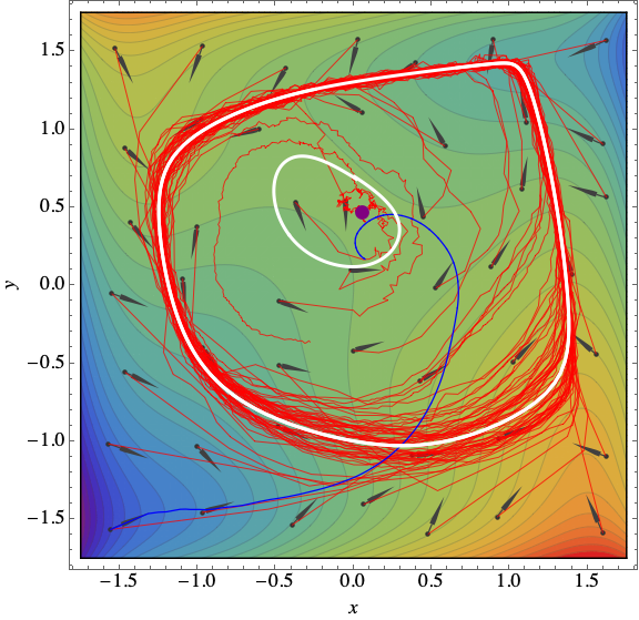
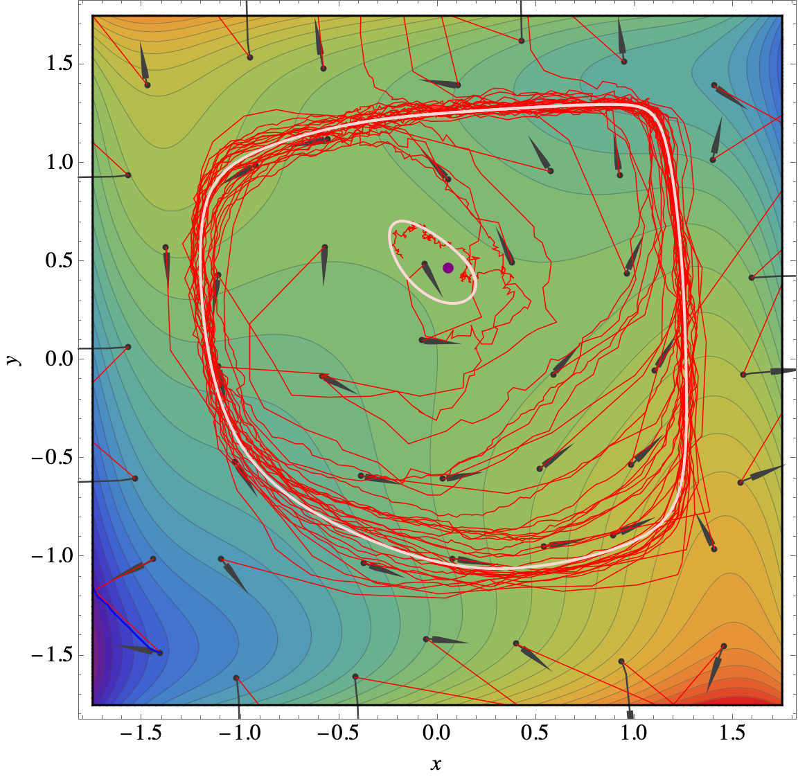
Figure 4. Spurious limits of second-order algorithms. From left to right: (a) SGA with $\lambda=0.2$ applied to (12); (b) ConO with $\lambda=0.2$ applied to (12).

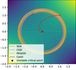
Figure 5. Spurious limits of min-max optimization algorithms from the same initialization. From left to right: (a) CGD for (12); (b) (OG/PEG) for (12); (c) Algorithms for (11).

D.4. Constant step-sizes

We report in Fig. 6 the behaviors of constant step-size RM schemes. In accord with our intuition, these schemes exhibit concentration behaviors around the attractors.

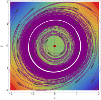
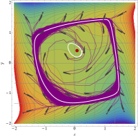
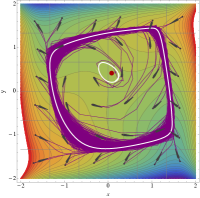
Figure 6. RM schemes with constant step-size $\gamma_{n}=0.01$ under the same initializations. From left to right: (a) (SGDA) for (11) with $\varepsilon=.1$; (b) (SGDA) for (12); (c) (SEG) for (11) with $\varepsilon=.1$; (d) (SEG) for (12).

D.5. Adaptive methods

We report in Fig. 7 the behaviors of popular adaptive algorithms for min-max optimization, including Adam [46] and its extra-gradient variant [30], both set to default hyperparameter values in PyTorch. The result reveals a potentially dangerous trend: while both Adam and ExtraAdam are able to somewhat mitigate cycling phenomena, this comes at the cost of converging to the max-min point $(0,0)$ of (11). In other words, the algorithm has converged, but to a very bad solution point – an observation which, in the terminology of Letcher [52], would mean that Adam is not a “reasonable” algorithm. Moreover, as all RM schemes, both adaptive methods fail to reach the “forsaken” solutions in Example 5.2.

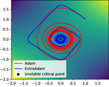
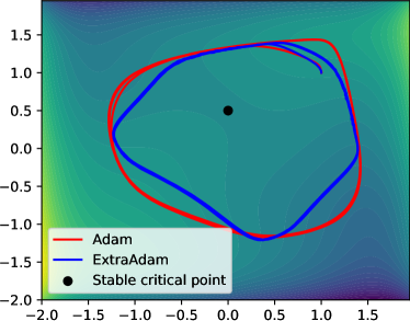
Figure 7. Adaptive algorithm. From left to right: (a) Adaptive algorithms for (11); (b) Adaptive algorithms for (12).

References

- Abernethy et al [2019] Abernethy J, Lai KA, Wibisono A (2019) Last-iterate convergence rates for min-max optimization. arXiv preprint arXiv:190602027
- Adolphs et al [2019] Adolphs L, Daneshmand H, Lucchi A, Hofmann T (2019) Local saddle point optimization: A curvature exploitation approach. In: The 22nd International Conference on Artificial Intelligence and Statistics, pp 486–495
- Arjovsky et al [2017] Arjovsky M, Chintala S, Bottou L (2017) Wasserstein gan. arXiv preprint arXiv:170107875
- Arrow et al [1958] Arrow KJ, Hurwicz L, Uzawa H (1958) Studies in linear and non-linear programming. Stanford University Press
- Balduzzi et al [2018] Balduzzi D, Racaniere S, Martens J, Foerster J, Tuyls K, Graepel T (2018) The mechanics of n-player differentiable games. In: International Conference on Machine Learning, pp 354–363
- Bauschke and Combettes [2017] Bauschke HH, Combettes PL (2017) Convex Analysis and Monotone Operator Theory in Hilbert Spaces, 2nd edn. Springer, New York, NY, USA
- Benaïm [1999] Benaïm M (1999) Dynamics of stochastic approximation algorithms. In: Azéma J, Émery M, Ledoux M, Yor M (eds) Séminaire de Probabilités XXXIII, Lecture Notes in Mathematics, vol 1709, Springer Berlin Heidelberg, pp 1–68
- Benaïm and Hirsch [1995] Benaïm M, Hirsch MW (1995) Dynamics of Morse-Smale urn processes. Ergodic Theory and Dynamical Systems 15(6):1005–1030
- Benaïm and Hirsch [1996] Benaïm M, Hirsch MW (1996) Asymptotic pseudotrajectories and chain recurrent flows, with applications. Journal of Dynamics and Differential Equations 8(1):141–176
- Benveniste et al [1990] Benveniste A, Métivier M, Priouret P (1990) Adaptive Algorithms and Stochastic Approximations. Springer
- Bertsekas and Tsitsiklis [2000] Bertsekas DP, Tsitsiklis JN (2000) Gradient convergence in gradient methods with errors. SIAM Journal on Optimization 10(3):627–642
- Borkar [2008] Borkar VS (2008) Stochastic Approximation: A Dynamical Systems Viewpoint. Cambridge University Press and Hindustan Book Agency
- Bowen [1975] Bowen R (1975) Omega limit sets of Axiom A diffeomorphisms. Journal of Differential Equations 18:333–339
- Burkholder [1973] Burkholder DL (1973) Distribution function inequalities for martingales. Annals of Probability 1(1):19–42
- Chambolle and Pock [2011] Chambolle A, Pock T (2011) A first-order primal-dual algorithm for convex problems with applications to imaging. Journal of mathematical imaging and vision 40(1):120–145
- Chavdarova et al [2019] Chavdarova T, Gidel G, Fleuret F, Lacoste-Julien S (2019) Reducing noise in GAN training with variance reduced extragradient. In: NeurIPS ’19: Proceedings of the 33rd International Conference on Neural Information Processing Systems
- Chiang et al [2012] Chiang CK, Yang T, Lee CJ, Mahdavi M, Lu CJ, Jin R, Zhu S (2012) Online optimization with gradual variations. In: COLT ’12: Proceedings of the 25th Annual Conference on Learning Theory
- Christopher and Li [2007] Christopher C, Li C (2007) Limit cycles of differential equations. Springer Science & Business Media
- Conley [1978] Conley CC (1978) Isolated Invariant Set and the Morse Index. American Mathematical Society, Providence, RI
- Daskalakis and Panageas [2018] Daskalakis C, Panageas I (2018) The limit points of (optimistic) gradient descent in min-max optimization. In: Advances in Neural Information Processing Systems, pp 9236–9246
- Daskalakis et al [2018] Daskalakis C, Ilyas A, Syrgkanis V, Zeng H (2018) Training GANs with optimism. In: ICLR ’18: Proceedings of the 2018 International Conference on Learning Representations
- Daskalakis et al [2020] Daskalakis C, Skoulakis S, Zampetakis M (2020) The complexity of constrained min-max optimization. arXiv preprint arXiv:200909623
- Domingo-Enrich et al [2020] Domingo-Enrich C, Jelassi S, Mensch A, Rotskoff G, Bruna J (2020) A mean-field analysis of two-player zero-sum games. arXiv preprint arXiv:200206277
- Facchinei and Pang [2003] Facchinei F, Pang JS (2003) Finite-Dimensional Variational Inequalities and Complementarity Problems. Springer Series in Operations Research, Springer
- Fiez and Ratliff [2020] Fiez T, Ratliff L (2020) Gradient descent-ascent provably converges to strict local minmax equilibria with a finite timescale separation. arXiv preprint arXiv:200914820
- Fiez et al [2019] Fiez T, Chasnov B, Ratliff LJ (2019) Convergence of learning dynamics in stackelberg games. arXiv preprint arXiv:190601217
- Flokas et al [2019] Flokas L, Vlatakis-Gkaragkounis EV, Piliouras G (2019) Poincaré recurrence, cycles and spurious equilibria in gradient-descent-ascent for non-convex non-concave zero-sum games. In: NeurIPS ’19: Proceedings of the 33rd International Conference on Neural Information Processing Systems
- Flokas et al [2021] Flokas L, Vlatakis-Gkaragkounis EV, Piliouras G (2021) Solving min-max optimization with hidden structure via gradient descent ascent. arXiv preprint arXiv:210105248
- Ge et al [2015] Ge R, Huang F, Jin C, Yuan Y (2015) Escaping from saddle points — Online stochastic gradient for tensor decomposition. In: COLT ’15: Proceedings of the 28th Annual Conference on Learning Theory
- Gidel et al [2019a] Gidel G, Berard H, Vignoud G, Vincent P, Lacoste-Julien S (2019a) A variational inequality perspective on generative adversarial networks. In: ICLR ’19: Proceedings of the 2019 International Conference on Learning Representations
- Gidel et al [2019b] Gidel G, Hemmat RA, Pezeshki M, Le Priol R, Huang G, Lacoste-Julien S, Mitliagkas I (2019b) Negative momentum for improved game dynamics. In: The 22nd International Conference on Artificial Intelligence and Statistics, pp 1802–1811
- Goodfellow et al [2014] Goodfellow IJ, Pouget-Abadie J, Mirza M, Xu B, Warde-Farley D, Ozair S, Courville A, Bengio Y (2014) Generative adversarial nets. In: NIPS ’14: Proceedings of the 28th International Conference on Neural Information Processing Systems
- Grimmer et al [2020a] Grimmer B, Lu H, Worah P, Mirrokni V (2020a) The landscape of nonconvex-nonconcave minimax optimization. arXiv preprint arXiv:200608667
- Grimmer et al [2020b] Grimmer B, Lu H, Worah P, Mirrokni V (2020b) Limiting behaviors of nonconvex-nonconcave minimax optimization via continuous-time systems. arXiv preprint arXiv:201010628
- Hall and Heyde [1980] Hall P, Heyde CC (1980) Martingale Limit Theory and Its Application. Probability and Mathematical Statistics, Academic Press, New York
- Heusel et al [2017] Heusel M, Ramsauer H, Unterthiner T, Nessler B, Hochreiter S (2017) Gans trained by a two time-scale update rule converge to a local nash equilibrium. In: Advances in neural information processing systems, pp 6626–6637
- Hsieh et al [2019a] Hsieh YG, Iutzeler F, Malick J, Mertikopoulos P (2019a) On the convergence of single-call stochastic extra-gradient methods. In: NeurIPS ’19: Proceedings of the 33rd International Conference on Neural Information Processing Systems, pp 6936–6946
- Hsieh et al [2020] Hsieh YG, Iutzeler F, Malick J, Mertikopoulos P (2020) Explore aggressively, update conservatively: Stochastic extragradient methods with variable stepsize scaling. In: NeurIPS ’20: Proceedings of the 34th International Conference on Neural Information Processing Systems
- Hsieh et al [2019b] Hsieh YP, Liu C, Cevher V (2019b) Finding mixed nash equilibria of generative adversarial networks. In: International Conference on Machine Learning, pp 2810–2819
- Iusem et al [2017] Iusem AN, Jofré A, Oliveira RI, Thompson P (2017) Extragradient method with variance reduction for stochastic variational inequalities. SIAM Journal on Optimization 27(2):686–724
- Jin et al [2019] Jin C, Netrapalli P, Jordan MI (2019) What is local optimality in nonconvex-nonconcave minimax optimization? arXiv preprint arXiv:190200618
- Juditsky et al [2011] Juditsky A, Nemirovski A, Tauvel C (2011) Solving variational inequalities with stochastic mirror-prox algorithm. Stochastic Systems 1(1):17–58
- Kamalaruban et al [2020] Kamalaruban P, Huang YT, Hsieh YP, Rolland P, Shi C, Cevher V (2020) Robust reinforcement learning via adversarial training with langevin dynamics. arXiv preprint arXiv:200206063
- Karras et al [2018] Karras T, Aila T, Laine S, Lehtinen J (2018) Progressive growing of gans for improved quality, stability, and variation. In: International Conference on Learning Representations
- Kiefer and Wolfowitz [1952] Kiefer J, Wolfowitz J (1952) Stochastic estimation of the maximum of a regression function. The Annals of Mathematical Statistics 23(3):462–466
- Kingma and Ba [2014] Kingma DP, Ba J (2014) Adam: A method for stochastic optimization. arXiv preprint arXiv:14126980
- Kupka [1963] Kupka I (1963) Contributiona la théorie des champs génériques. Contributions to differential equations 2:457–484
- Kushner and Clark [1978] Kushner HJ, Clark DS (1978) Stochastic Approximation Methods for Constrained and Unconstrained Systems. Springer
- Kushner and Huang [1981] Kushner HJ, Huang H (1981) Asymptotic properties of stochastic approximations with constant coefficients. SIAM Journal on Control and Optimization 19(1):87–105
- Kushner and Yin [1997] Kushner HJ, Yin GG (1997) Stochastic approximation algorithms and applications. Springer-Verlag, New York, NY
- Lee [2003] Lee JM (2003) Introduction to Smooth Manifolds. No. 218 in Graduate Texts in Mathematics, Springer-Verlag, New York, NY
- Letcher [2020] Letcher A (2020) On the impossibility of global convergence in multi-loss optimization. arXiv preprint arXiv:200512649
- Liu et al [2019a] Liu M, Mroueh Y, Ross J, Zhang W, Cui X, Das P, Yang T (2019a) Towards better understanding of adaptive gradient algorithms in generative adversarial nets. arXiv preprint arXiv:191211940
- Liu et al [2019b] Liu S, Lu S, Chen X, Feng Y, Xu K, Al-Dujaili A, Hong M, Obelilly UM (2019b) Min-max optimization without gradients: Convergence and applications to adversarial ml. arXiv preprint arXiv:190913806
- Ljung [1977] Ljung L (1977) Analysis of recursive stochastic algorithms. IEEE Trans Autom Control 22(4):551–575
- Madry et al [2018] Madry A, Makelov A, Schmidt L, Tsipras D, Vladu A (2018) Towards deep learning models resistant to adversarial attacks. In: ICLR ’18: Proceedings of the 2018 International Conference on Learning Representations
- Malitsky and Tam [2020] Malitsky Y, Tam MK (2020) A forward-backward splitting method for monotone inclusions without cocoercivity. SIAM Journal on Optimization 30(2):1451–1472
- Mazumdar et al [2020] Mazumdar E, Ratliff LJ, Sastry SS (2020) On gradient-based learning in continuous games. SIAM Journal on Mathematics of Data Science 2(1):103–131
- Mertikopoulos et al [2019] Mertikopoulos P, Lecouat B, Zenati H, Foo CS, Chandrasekhar V, Piliouras G (2019) Optimistic mirror descent in saddle-point problems: Going the extra (gradient) mile. In: ICLR ’19: Proceedings of the 2019 International Conference on Learning Representations
- Mertikopoulos et al [2020] Mertikopoulos P, Hallak N, Kavis A, Cevher V (2020) On the almost sure convergence of stochastic gradient descent in non-convex problems. Advances in Neural Information Processing Systems 33
- Mescheder et al [2017] Mescheder L, Nowozin S, Geiger A (2017) The numerics of gans. In: Advances in Neural Information Processing Systems, pp 1825–1835
- Mokhtari et al [2019a] Mokhtari A, Ozdaglar A, Pattathil S (2019a) A unified analysis of extra-gradient and optimistic gradient methods for saddle point problems: proximal point approach. https://arxiv.org/abs/1901.08511v2
- Mokhtari et al [2019b] Mokhtari A, Ozdaglar A, Pattathil S (2019b) A unified analysis of extra-gradient and optimistic gradient methods for saddle point problems: Proximal point approach. arXiv preprint arXiv:190108511
- Nagarajan and Kolter [2017] Nagarajan V, Kolter JZ (2017) Gradient descent gan optimization is locally stable. In: Advances in neural information processing systems, pp 5585–5595
- Naveiro and Insua [2019] Naveiro R, Insua DR (2019) Gradient methods for solving stackelberg games. In: International Conference on Algorithmic DecisionTheory, Springer, pp 126–140
- Nemirovski [2004a] Nemirovski A (2004a) Prox-method with rate of convergence o (1/t) for variational inequalities with lipschitz continuous monotone operators and smooth convex-concave saddle point problems. SIAM Journal on Optimization 15(1):229–251
- Nemirovski [2004b] Nemirovski AS (2004b) Prox-method with rate of convergence for variational inequalities with Lipschitz continuous monotone operators and smooth convex-concave saddle point problems. SIAM Journal on Optimization 15(1):229–251
- Nesterov [2004] Nesterov Y (2004) Introductory Lectures on Convex Optimization: A Basic Course. No. 87 in Applied Optimization, Kluwer Academic Publishers
- Pearlmutter [1994] Pearlmutter BA (1994) Fast exact multiplication by the hessian. Neural computation 6(1):147–160
- Pemantle [1990] Pemantle R (1990) Nonconvergence to unstable points in urn models and stochastic aproximations. Annals of Probability 18(2):698–712
- Pemantle [1992] Pemantle R (1992) Vertex-reinforced random walk. Probability Theory and Related Fields 92:117–136
- Peng et al [2020] Peng W, Dai YH, Zhang H, Cheng L (2020) Training gans with centripetal acceleration. Optimization Methods and Software pp 1–19
- Phelps [1993] Phelps RR (1993) Convex Functions, Monotone Operators and Differentiability, 2nd edn. Lecture Notes in Mathematics, Springer-Verlag
- Pinto et al [2017] Pinto L, Davidson J, Sukthankar R, Gupta A (2017) Robust adversarial reinforcement learning. In: ICML ’17: Proceedings of the 34th International Conference on Machine Learning
- Popov [1980] Popov LD (1980) A modification of the Arrow–Hurwicz method for search of saddle points. Mathematical Notes of the Academy of Sciences of the USSR 28(5):845–848
- Rakhlin and Sridharan [2013] Rakhlin A, Sridharan K (2013) Online learning with predictable sequences. In: COLT ’13: Proceedings of the 26th Annual Conference on Learning Theory
- Robbins and Monro [1951] Robbins H, Monro S (1951) A stochastic approximation method. Annals of Mathematical Statistics 22:400–407
- Robinson [1998] Robinson C (1998) Dynamical systems: stability, symbolic dynamics, and chaos. CRC press
- Rockafellar [1976] Rockafellar RT (1976) Monotone operators and the proximal point algorithm. SIAM journal on control and optimization 14(5):877–898
- Schäfer and Anandkumar [2019] Schäfer F, Anandkumar A (2019) Competitive gradient descent. In: Advances in Neural Information Processing Systems, pp 7623–7633
- Shub [1987] Shub M (1987) Global Stability of Dynamical Systems. Springer-Verlag, Berlin
- Smale [1963] Smale S (1963) Stable manifolds for differential equations and diffeomorphisms. Annali della Scuola Normale Superiore di Pisa-Classe di Scienze 17(1-2):97–116
- Spall [1992] Spall JC (1992) Multivariate stochastic approximation using a simultaneous perturbation gradient approximation. IEEE Trans Autom Control 37(3):332–341
- Teschl [2012] Teschl G (2012) Ordinary differential equations and dynamical systems, vol 140. American Mathematical Soc.
- Wiggins [2003] Wiggins S (2003) Introduction to applied nonlinear dynamical systems and chaos, vol 2. Springer Science & Business Media
- Yadav et al [2017] Yadav A, Shah S, Xu Z, Jacobs D, Goldstein T (2017) Stabilizing adversarial nets with prediction methods. arXiv preprint arXiv:170507364