Numerical evidence towards a positive answer to Morrey’s problem

Abstract

We report on numerical experiments suggesting that rank-one convexity imples quasiconvexity in the planar case. We give a simple heuristic explanation of our findings.

Keywords: Quasiconvexity, Rank-one convexity, Gradient Young measures, Laminates. 2010 MSC: 49J45.

1   Introduction

An important problem in the vectorial Calculus of Variations is to characterize the integrands $f\colon\mathbb{R}^{m\times n}\to\mathbb{R}$ for which the functional

$$\mathcal{F}[u]\equiv\int_{\Omega}f(\textup{D}u(x))\,\textup{d}x,\qquad\textup{where }u\colon\Omega\subseteq\mathbb{R}^{n}\to\mathbb{R}^{m}\textup{ and }m,n\geq 2,$$

is lower semicontinuous with respect to the weak topology in an appropriate Sobolev space; this is the natural condition for existence of minimizers through the Direct Method.

In his seminal work [28], Morrey recognized that the weak lower semicontinuity of $\mathcal{F}$ is essentially equivalent to a weak notion of convexity, called quasiconvexity, on $f$. Despite many efforts in the last five decades, an explicit description of quasiconvex functions remains elusive: for instance, there are fourth-order polynomials whose quasiconvexity has been neither proved nor disproved. Such a description would be relevant not only in the Calculus of Variations but also in other areas of analysis [17, 22, 27, 39].

Quasiconvexity has been mostly studied in relation with polyconvexity [3] and rank-one convexity; these are respectively stronger and weaker notions that are much easier to tackle [6]. We will focus on the relation between quasiconvexity and rank-one convexity. It is useful to consider certain classes of measures that can be seen as being dual to these notions: gradient Young measures and laminates are, respectively, the probability measures that satisfy Jensen’s inequality with respect to quasiconvex and rank-one convex functions; see [31] for more details.

The following remains one of the main open problems in the Calculus of Variations:

1.1 Question.

Are rank-one convex functions quasiconvex? Equivalently, let $\nu$ be a compactly supported gradient Young measure in $\mathbb{R}^{m\times n}$; is $\nu$ a laminate?

Quesion 1.1 is usually referred to as Morrey’s problem. It seems that Morrey himself was not sure about what the answer to Question 1.1 should be [28, 29]. A fundamental example of Šverák [37] shows that the answer is negative if $m\geq 3$, $n\geq 2$ and more recently Grabovsky [13] obtained a different example when $m=8$ and $n=2$. Šverák’s example is a polynomial of degree four; Grabovsky’s example, although analytically more complicated, has the advantage of being 2-homogeneous and invariant under the right-action of $\textup{SO}(2)$. Question 1.1 remains open in the case of low-dimensional targets, i.e. when $m=2$ and $n\geq 2$. There is some partial evidence suggesting that the answer might be positive in this case, see e.g. the landmark results of [11, 16, 24, 30]. However, and despite remarkable progress, it is by no means clear that the answer should be positive even in low dimensions.

Since the analytic study of quasiconvexity remains incredibly challenging, it is natural to look for numerical evidence instead: that is the goal of this note. In line with the ideas from [37], we fix a Lipschitz deformation $u\colon\mathbb{T}^{n}\to\mathbb{R}^{m}$ whose gradient has finite image and we look for rank-one convex functions falsifying Jensen’s inequality with respect to $\textup{D}u$. Given such a deformation, it suffices to consider the rank-one convex envelopes of functions of the form

$$f(A)=\begin{cases}g(A)&A\in[\textup{D}u]\\ 2&\textup{otherwise }\end{cases},$$

where $[\textup{D}u]$ denotes the essential range of $\textup{D}u\in L^{\infty}(\Omega,\mathbb{R}^{m\times n})$ and $g\colon[\textup{D}u]\to[-1,1]$ is any function. In other words, for a deformation such that $[\textup{D}u]$ is finite the task of looking for counterexamples is a finite-dimensional problem. As a small technical remark we note that it is important that $f$ only takes finite values; it is easy to build examples of rank-one convex non-quasiconvex functions if the value $+\infty$ is allowed [2].

Arbitrary deformations can be approximated by linear combinations of plane waves and we will consider finite sums of such waves, see Section 3. Our choice is inspired by James’s interpretation of Šverák’s example, where three waves suffice to build a counterexample.

Numerical searches for counterexamples to Question 1.1 have been undertaken before [7, 8, 14]. The strategy of these papers is the opposite from the one we pursue here: they fix a rank-one convex function $f$ and look for deformations for which $f$ does not satisfy Jensen’s inequality. The main problem of this approach is that explicit rank-one convex non-polyconvex functions are rare and the available examples are relatively simple and have many symmetries. Our procedure is much more general, since our deformations are sampled randomly and the rank-one convex functions have as little structure as possible.

By homogenization, the gradient of a Lipschitz deformation $u\colon\mathbb{T}^{n}\to\mathbb{R}^{m}$ generates a gradient Young measure, which has finite support if $[\textup{D}u]$ is finite; thus our goal is to determine whether this measure is a laminate. Hence, we are naturally led to consider:

1.2 Question ([23]).

Is there an effective algorithm to decide whether a given probability measure supported on a finite subset of $\mathbb{R}^{m\times n}$ is a laminate?

Deciding whether a given measure is a laminate is difficult, as in principle one has to test Jensen’s inequality with all rank-one convex functions [33]. One possible way of circumventing this issue is to consider just the extremal rank-one convex functions [15]; however, the general structure of these functions remains unclear. A different approach is to use a discretized version of the Kohn–Strang algorithm [25] and in Section 2 we show that this yields a partially satisfying answer to Question 1.2. We rely on the convergence of approximations to the rank-one convex envelope, which were proved in [5, 9, 10, 32], see also [40] for particular examples. We remark that the related problem of calculating the rank-one convex hull of a set still remains poorly understood, see [1] and the references therein.

To conclude the introduction, let us return to Question 1.1 and discuss the numerical results presented in this note. We randomly sample deformations given by the sum of $N$ plane waves, for some $N\in\{3,4,5\}$; the cases $N=1,2$ are not interesting and for $N\geq 6$ we already have that $\#[\textup{D}u]\geq 64$, so the space of functions $g\colon[\textup{D}u]\to[-1,1]$ becomes very high-dimensional. Our approach finds many counterexamples, similar to the ones in [37], when $m\geq 3$; however, and despite sampling thousands of different deformations, none where found when $m=2$. In this last case, we observe that on average it is easier to check that a given function does not yield a counterexample to Question 1.1 as $N$ increases. We give a basic heuristic explanation of these findings: for plane wave expansions, the rank-one geometry of the set $[\textup{D}u]$ is drastically different in the cases $m=3$ and $m=2$ and, in the latter, the geometry becomes much richer as $N$ increases. Our considerations are inspired by the very interesting results of Sebestyén–Székelyhidi [36], where the authors tap into this structure to prove that no counterexamples arise when $m=2$ and $N=3$, see also [34].

Acknowledgements.

A.G. would like to thank Vladimír Šverák for a very interesting conversation about Morrey’s problem and, in particular, for the suggestion of conducting a numerical experiment roughly along the lines of the one described in Section 5. A.G. would also like to thank Jan Kristensen for countless hours of discussion about the problems addressed here. A.G. was sponsored by [EP/L015811/1]. R.TdC. was sponsored by [EP/L016516/1].

2   Deciding whether a measure is a laminate

In this section we discuss Question 1.2: throughout $\nu$ is a fixed probability measure with support on a finite set $K\subset\mathbb{R}^{m\times n}$. In this section we use a discretized version of the Kohn–Strang algorithm to show the following:

2.1 Proposition.

Let $\nu$ be a probability measure supported in a finite set of points in $\mathbb{R}^{m\times n}$. The problem of deciding whether $\nu$ is a laminate is semidecidable, i.e. there is an algorithm which terminates in finite time with a positive answer if $\nu$ is a laminate.

To prove this, we will resort to Pedregal’s Theorem [33]: $\nu$ is a laminate if and only if

(2.2) $$f^{\textup{rc}}(\overline{\nu})\leq\langle\nu,f\rangle,\hskip 14.22636pt\overline{\nu}\equiv\langle\nu,\textup{id}\rangle$$

for all continuous $f\colon\mathbb{R}^{m\times n}\to\mathbb{R}$, where $f^{\textup{rc}}$ denotes the rank-one convex envelope of $f$.

2.3 Lemma.

If $\nu$ is not a laminate there is $g\colon K\to[-1,1]$ such that, for $0<\delta<c(K,n,m)$ small enough, the continuous function $f_{\delta}\colon\mathbb{R}^{m\times n}\to[-1,2]$, defined by

(2.4) $$f_{\delta}(A)\equiv\begin{cases}g(A_{0})+\frac{2-g(A_{0})}{\delta}|A-A_{0}|&\textup{if }|A-A_{0}|\leq\delta\textup{ for some }A_{0}\in K\\ 2&\textup{otherwise},\end{cases}$$

satisfies $f^{\textup{rc}}_{\delta}(\overline{\nu})>\langle\nu,f^{\textup{rc}}_{\delta}\rangle$.

Although this is not needed, note that $\lim_{\delta\to 0}f_{\delta}=f_{0}\equiv g\mathbbm{1}_{K}+2\times\mathbbm{1}_{\mathbb{R}^{m\times n}\backslash K}$ pointwise.

[Proof:]Since $\nu$ is not a laminate, there is $\tilde{g}\colon\mathbb{R}^{m\times n}\to\mathbb{R}$ rank-one convex and such that $g(\overline{\nu})>\langle\nu,g\rangle$; by scaling, we can assume that $\tilde{g}([-2,2]^{mn})\subseteq[-1,1].$ Since $\tilde{g}$ is rank-one convex it is locally Lipschitz and, see [4],

$$\textup{Lip}(\tilde{g},[-1,1]^{mn})\leq\min\{m,n\}\textup{\,osc}(\tilde{g},[-2,2]^{mn})\leq 2\min\{m,n\}.$$

Let us take $g=\tilde{g}|_{K}$, $\delta\leq\frac{1}{2}\min\{|X_{1}-X_{2}|\mathrel{\mathop{\mathchar 58\relax}}X_{1},X_{2}\in K\}$ so that $f_{\delta}$ is well-defined and, in addition, we require that $\delta<(2\min\{m,n\})^{-1}$. Thus, for $A\in B_{\delta}(A_{0})$ and $A_{0}\in K$,

$$\tilde{g}(A)\leq\tilde{g}(A_{0})+2\min\{m,n\}|A-A_{0}|\leq\tilde{g}(A_{0})+\frac{1}{\delta}|A-A_{0}|\leq f_{\delta}(A).$$

This shows that $f_{\delta}\geq\tilde{g}$; since $g$ is rank-one convex, also $f_{\delta}^{\textup{rc}}\geq\tilde{g}$ and so

$$f^{\textup{rc}}_{\delta}(\overline{\nu})\geq\tilde{g}(\overline{\nu})>\langle\nu,g\rangle=\langle\nu,f_{\delta}^{\textup{rc}}\rangle.$$

Lemma 2.3 shows that in order to decide whether $\nu$ is a laminate one has to explore the finite-dimensional space of functions $g\colon K\to[-1,1]$. In order to compute an approximation of $f^{\textup{rc}}_{\delta}$ we use a discrete version of the Kohn–Strang algorithm [25].

2.5 Algorithm.

We fix $\delta>0$ small enough so that we do not need to worry about it; thus we drop the subscript $\delta$. By translation invariance we can assume that $\overline{\nu}=0$. Then:

1. Fix an odd integer $L$, consider the grid $\mathcal{G}_{L}\equiv\frac{1}{L}\mathbb{Z}^{mn}\cap[-1,1]^{mn}$, and choose a finite set of directions $\mathcal{D}$ consisting of rank-one matrices which are in $\mathcal{G}_{L}$.

2. Set $f^{\textup{rc},0}_{L,\mathcal{D}}\mathrel{\mathop{\mathchar 58\relax}}=f$ and, for $A\in\mathcal{G}_{L}$,

   $$f^{\textup{rc},i+1}_{L,\mathcal{D}}(A)=\min_{\begin{subarray}{c}X\in\mathcal{D}\mathrel{\mathop{\mathchar 58\relax}}A\pm X\in\mathcal{G}_{L}\end{subarray}}\left\{\frac{f^{\textup{rc},i}_{L,\mathcal{D}}(A+X)+f^{\textup{rc},i}_{L,\mathcal{D}}(A-X)}{2},f^{\textup{rc},i}_{L,\mathcal{D}}(A)\right\}.$$

   We terminate the algorithm if either the maximum difference between iterates stabilizes or $f^{\textup{rc},i}_{L,\mathcal{D}}$ satisfies Jensen’s inequality with respect to $\nu$.

Let $f^{\textup{rc},i}$ be the $i$-th Kohn–Strang iterate, i.e. $f^{\textup{rc},i}$ is defined inductively by $f^{\textup{rc},0}=f$ and

$$f^{\textup{rc},i}(A)=\inf\left\{\lambda f^{\textup{rc},i-1}(X)+(1-\lambda)f^{\textup{rc},i-1}(Y)\mathrel{\mathop{\mathchar 58\relax}}\lambda X+(1-\lambda)Y=A,\textup{rank}(X-Y)=1\right\},$$

where $\lambda$ runs over $(0,1)$. Clearly, for $A\in\mathcal{G}_{L}$, $f^{\textup{rc},i}(A)\leq f^{\textup{rc},i}_{L,\mathcal{D}}(A)\leq f(A),$ and so if $f^{\textup{rc},i}_{L,\mathcal{D}}$ satisfies Jensen’s inequality with respect to $\nu$, $f_{\delta}$ satisfies (2.2). Conversely, we have:

2.6 Proposition.

Let $f^{\textup{rc}}_{L,\mathcal{D}}\equiv\lim_{i\to\infty}f^{\textup{rc},i}_{L,\mathcal{D}}$. Then $f^{\textup{rc}}_{L,\mathcal{D}}$ converges uniformly to $f_{\delta}^{\textup{rc}}$ as $L\to\infty$ and as the largest angle between any rank-one matrix and its best approximation in $\mathcal{D}$ goes to zero.

For a proof see [32]. Note that we take $0<\delta<c(m,n,K)$ and that $f_{\delta}$ is continuous, so their results apply. It is clear that combining Lemma 2.3 with Proposition 2.6, we deduce Proposition 2.1.

3   Gradient Young measures versus laminates

In this section we adress Question 1.1. Recall that a function $f\colon\mathbb{R}^{m\times n}\to\mathbb{R}$ is said to be quasiconvex if, for all $A\in\mathbb{R}^{m\times n}$,

(3.1) $$f(A)\leq\int_{\mathbb{T}^{n}}f(A+\textup{D}\varphi(x))\,\textup{d}x\hskip 14.22636pt\textup{ for all }\varphi\in C^{\infty}(\mathbb{T}^{n},\mathbb{R}^{m}).$$

Equivalently, $f$ is quasiconvex if and only if $f(\overline{\nu})\leq\langle\nu,f\rangle$, where $\nu$ is any compactly supported gradient Young measure [20, 31].

We want to test the inequality (3.1) with deformations of the form

(3.2) $$\varphi(x)=\sum_{i=1}^{N}a_{i}s(x\cdot n_{i}+c_{i}),$$

where $N\in\mathbb{N}$, $a_{i}\in\mathbb{R}^{m},n_{i}\in\mathbb{Z}^{n}$ are vectors, $c_{i}\in\mathbb{R}$ are phases and $s$ is the 1-periodic sawtooth function, defined for $t\in[0,1]$ by $s(t)=t1_{[0,1/2]}(t)+(1-t)1_{[1/2,1]}(t)$. The idea of approximating an arbitrary deformation with a simplified deformation with the form (3.2) is known in the Applied Harmonic Analysis literature as a ridgelet expansion [35]. We remark as a somewhat inconvenient fact that orthonormal ridgelet bases in $L^{2}$, just like Fourier series, are never unconditional bases in $L^{p}$ for $p\neq 2$, although we do not prove this here.

The advantage of an expansion as in (3.2) is that, with $h\equiv s^{\prime}$ being the Haar wavelet,

$$\textup{D}\varphi(x)=\sum_{i=1}^{N}h(x\cdot n_{i}+c_{i})\,a_{i}\otimes n_{i};$$

hence the gradient $\textup{D}\varphi$ takes values in a finite set. In our context, considering plane-wave expansions as in (3.2) is a classical idea, and we are motivated by James’ interpretation of Šverák’s example [31], see also [27, §31] and [34, 36]. Moreover, $\varphi$ generates a homogeneous gradient Young measure $\nu$, which takes the form

(3.3) $$\nu=\sum_{\varepsilon\in\{-1,1\}^{N}}\nu_{\varepsilon}\delta_{X_{\varepsilon}},$$

where we defined the weights $\nu_{\varepsilon}$ and the matrices $X_{\varepsilon}$ as

(3.4) $$\nu_{\varepsilon}\equiv|\{x\in\mathbb{T}^{2}\mathrel{\mathop{\mathchar 58\relax}}h(x\cdot n_{i}+c_{i})=\varepsilon_{i},i=1,\dots,N\}|,\hskip 14.22636ptX_{\varepsilon}\equiv\sum_{i=1}^{N}\varepsilon_{i}a_{i}\otimes n_{i}.$$

Note that $\nu_{\varepsilon}$ depends on $n_{i}$ but not on $a_{i}$. Furthermore, the measure $\nu$ has barycentre zero.

For the sake of conciseness, we introduce the following definition:

3.5 Definition.

For $N\in\mathbb{N}$, we say that $f\colon\mathbb{R}^{m\times n}\to\mathbb{R}$ is $N$-wave quasiconvex at zero if

$$f(0)\leq\sum_{\varepsilon\in\{-1,1\}^{N}}\nu_{\varepsilon}f(X_{\varepsilon})$$

for all $(a_{i},n_{i},c_{i})\in\mathbb{R}^{m}\times\mathbb{Z}^{n}\times\mathbb{R}$, where $\nu_{\varepsilon}$ and $X_{\varepsilon}$ are defined by (3.4). Moreover, $f$ is $N$-wave quasiconvex if, for any $A\in\mathbb{R}^{m\times n}$, the function $f(\cdot-A)$ is $N$-wave quasiconvex at zero.

It seems that variants of this notion were studied in [19] for $N=3,4$. By periodicity, in Definition 3.5 we can assume that $c_{1}=\dots=c_{I}=0$ where $I=\min\{n,N\}$. We have:

3.6 Proposition.

$f$ is quasiconvex if and only if it is $N$-wave quasiconvexity for all $N$.

[Proof:]We prove that if $f$ is $N$-wave quasiconvex at zero it is quasiconvex at zero, as the converse is clear. We rely on the following standard fact: for $\varphi\in C^{\infty}(\mathbb{T}^{n},\mathbb{R}^{m})$ there is a sequence $\varphi_{j}$ of the form (3.2) which converges to $\varphi$ strongly in $W^{1,\infty}(\mathbb{T}^{n},\mathbb{R}^{m})$. For a quantitative version of this fact when $m=1$ see e.g. [12], although there the authors take several different functions $s_{i}$, for $i=1,\dots N$, instead of a fixed sawtooth function; regardless, any $s_{i}$ can be approximated by scaled and translated copies of $s$. The general case $m>1$ follows by straightforward argument and we omit it.

Let $\nu_{j}$ be the gradient Young measure generated by the deformation $\varphi_{j}$; by assumption,

$$f(0)=f(\overline{\nu}_{j})\leq\langle\nu_{j},f\rangle=\int_{\mathbb{T}^{n}}f(\textup{D}\varphi_{j})\,\textup{d}x.$$

Since $\varphi_{j}\to\varphi$ in $W^{1,\infty}(\mathbb{T}^{n},\mathbb{R}^{m})$, we see that $f(0)\leq\int_{\mathbb{T}^{n}}f(\textup{D}\varphi)\,\textup{d}x.$ Thus $f$ is quasiconvex at zero.

The following theorem gathers several results from the literature.

3.7 Theorem.

$N$-wave quasiconvexity has the following properties:

1. 1-wave quasiconvexity is equivalent to rank-one convexity;

2. 2-wave quasiconvexity is equivalent to rank-one convexity;

3. if $m\geq 3,n\geq 2$ then 3-wave quasiconvexity is different from rank-one convexity and is a nonlocal property;

4. if $m=n=2$ then 3-wave quasiconvexity is implied by rank-one convexity.

[Proof:](a) follows straightforwardly, (b) follows by [36, Lemma 2.1], (c) follows from the example in [37] together with an adaptation of the arguments in [26] and (d) is the main result of [36].

4   Counting rank-one connections

The behaviour of gradients of maps changes dramatically from the higher-dimensional to the planar case [11, 18, 24]. One of the basic explanations for this difference is that the relative size of the cone

$$\Lambda\equiv\{A\in\mathbb{R}^{m\times 2}\mathrel{\mathop{\mathchar 58\relax}}\textup{rank}\,A\leq 1\}$$

is much larger when $m=2$ than when $m\geq 3$: for instance, it separates the matrix space into two components in the former case.

The previous insight is also relevant towards the goal of understanding the behaviour of the particular deformations of Section 3. In fact, the proof of Theorem 3.7(d) in [36] also explores the fact that $\Lambda$ is large: using arguments somewhat in the spirit of [38], the abundance of rank-one connections is used to build complicated laminates supported in the 3-cube $\{X_{\varepsilon}\}_{\varepsilon\in\{-1,1\}^{3}}$. In view of Proposition 3.6 it is natural to ponder what can be said for a general $N>3$.

In this section our goal is to roughly quantify the number of rank-one connections between points in the lamination hull of the $N$-cube. Our observations are merely heuristic, i.e. we do not provide any proofs, and they are the consequence of analysing thousands of computer-generated random configurations.

For a given choice of matrices $X_{\varepsilon}$ as in (3.4), let us write

$$K_{N}\equiv\{X_{\varepsilon}\mathrel{\mathop{\mathchar 58\relax}}\varepsilon\in\{-1,1\}^{N}\}\subset\mathbb{R}^{m\times 2},\qquad Q_{N}\equiv[-1,1]^{N}\subset\mathbb{R}^{N}.$$

We can visualise $K_{N}$ as the vertices of the $N$-cube $Q_{N}$ by considering the map $X_{\varepsilon}\mapsto\varepsilon$. Note, however, that for $N>2m$ the map $\varepsilon\mapsto X_{\varepsilon}$ cannot be an embedding.

Let us denote by $K_{N}^{\textup{lc},i}$ the usual $i$-th lamination convex hull of $K_{N}$, see [31] for the definition. Since the edges of the cube correspond to rank-one segments, it is clear that, under the above identification, $K_{N}^{\textup{lc},i}$ contains the $i$-skeleton of $Q_{N}$: for instance, $K_{N}^{\textup{lc},1}$ contains the edges of the cube, $K_{N}^{\textup{lc},2}$ contains the faces, and so on.

We say that $X_{\varepsilon}$ and $X_{\varepsilon^{\prime}}$ are neighbours if $\varepsilon$ and $\varepsilon^{\prime}$ are adjacent vertices in $Q_{N}$. Generically, each vertex $X_{\varepsilon}$ is rank-one connected only to its $N$ neighbours and thus $K_{N}^{\textup{lc},1}$ is in fact the 1-skeleton of the $N$-cube, i.e. it consists of the vertices and the edges $E_{N}\equiv K_{N}^{\textup{lc},1}\backslash K_{N}$; note that each edge is an open segment parallel to a rank-one line.

We now want to compare $K_{N}^{\textup{lc},2}$ with the 2-skeleton of the $N$-cube. We call a rank-one connection trivial if it exists in the 2-skeleton of the $N$-cube. A vertice is trivially connected to the $N$ edges that have that vertex as one of their endpoints. An edge, which we write in the form $\{(\varepsilon_{1},\dots,\varepsilon_{i-1},t,\varepsilon_{i+1},\dots,\varepsilon_{N})\mathrel{\mathop{\mathchar 58\relax}}t\in[0,1]\}$, is trivially connected to the $N-1$ edges that arise by flipping the sign of one of the $\varepsilon_{j}$, for $j\neq i$.

Let us consider a fixed deformation. We count, for each vertice and each edge, the number of non-trivial edges to which it is rank-one connected; thus we find two vectors of natural numbers, one with length $N$, the other with $N2^{N-1}$. For these vectors we calculate their mean deviation. Finally, sampling randomly thousands of deformations, we get approximate values for the average number of connections, see Tables 4.1 and 4.2.

	$m=2$	$m=3$
$N=3$	0.95 (0.47)	0 (0)
$N=4$	4.79 (1.57)	0 (0)
$N=5$	15.59 (3.65)	0 (0)
$N=6$	41.70 (8.31)	0 (0)

Table 4.1: Average number (and average mean deviation) of the number of non-trivial edges to which a vertice is rank-one connected.

	$m=2$	$m=3$
$N=3$	2.90 (0.63)	0 (0)
$N=4$	12.50 (2.39)	0 (0)
$N=5$	36.78 (7.06)	0 (0)
$N=6$	92.17 (18.28)	0 (0)

Table 4.2: Average number (and average mean deviation) of the number of non-trivial edges to which an edge is rank-one connected.

4.1 Remark.

We would like to make a few points concerning Tables 4.1 and 4.2:

1. The values obtained should be understood in a probabilistic sense: it is not true that, when $m=3$, there are never non-trivial connections. In fact, if we randomise vectors $a_{i}\in(\mathbb{Z}\cap[-L,L])^{3},n_{i}\in(\mathbb{Z}\cap[-L,L])^{2}$ with $L$ a small number, say $L=5$, then we find non-trivial rank-one connections in many of the corresponding configurations.

2. The low average mean deviations in the tables show that the connections are not concentrated in a few vertices or edges; see also Figure 4.1.

3. When $m=2$, an increase in $N$ also increases the number of connections dramatically. Thus, although the set $K_{N}$ becomes exponentially more complicated as $N$ increases, the geometry of its rank-one lines also becomes much richer.

4.2 Remark.

Rank-one lines are very fragile: even if sometimes rank-one connections exist, they are easily destroyed by small perturbations [21]. It is therefore more appropriate to consider the rank-one convex hull, which is often much larger than the lamination convex hull, albeit it is also much more difficult to calculate.

What we find the most remarkable about Tables 4.1 and 4.2 is not the fact that there are almost no rank-one connections when $m=3$ but rather that there are so many connections when $m=2$. Thus, in low-dimensions, simple lamination seems to be a viable option to produce very complex gradients. We believe that Tables 4.1 and 4.2 can be taken as partial evidence towards a positive answer to Question 1.1 when $m=n=2$.

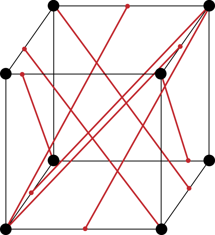
(a) Non-trivial vertice-edge connections.

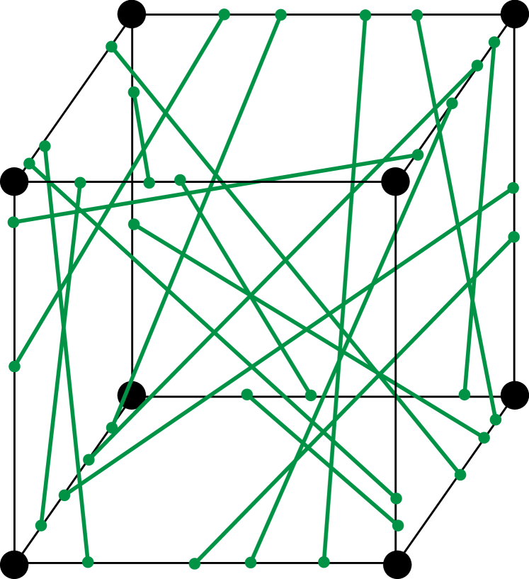
(b) Non-trivial edge-edge connections.

Figure 4.1: Depiction of a “typical” configuration when $N=3$ and $m=2$, with an average of 1 vertice-edge connection per vertex and 3 edge-edge connections per edge. Each line denotes the existence of at least one point in the edge which is rank-one connected.

5   Numerical search for counterexamples to Morrey’s problem

In this section we report on numerical experiments which bring together Sections 2 and 3. Our goal was to find numerical evidence towards a resolution of Question 1.1.

We set $n=2$ and run the following algorithm:

5.1 Algorithm.

Fix $L,N\in\mathbb{N}$, with $L$ odd and sufficiently large, and a threshold $\gamma\in[0,1]$. Set $\mathcal{G}_{L}\equiv\frac{1}{L}\mathbb{Z}^{2m}\cap[-1,1]^{2m}$ and choose a finite set of directions $\mathcal{D}$ consisting of rank-one matrices which are in $\mathcal{G}_{L}$. Then:

1. Randomly generate a set of directions, $(n_{i})_{i=1}^{N}$ in $([-L,L]\cap\mathbb{Z})^{2}$. Check that $n_{i}$ and $n_{j}$ are linearly independent for $i\neq j$; if not, repeat the previous instruction.

2. For each $(n_{i})_{i=1}^{N}$, randomly generate a set of phases, $(c_{i})_{i=1}^{N}\in\mathbb{R}$. The set $(n_{i},c_{i})_{i=1}^{N}$ determines the weights, $(\nu_{\varepsilon})_{\varepsilon}$, at each point in the support of the measure, see (3.4).

3. Randomly generate a set of vectors $(a_{i})_{i=1}^{N}$ in $(\frac{1}{L}\mathbb{Z}\cap[-1,1])^{m}$. Check that $a_{i}\neq 0$ for all $i$ and that the matrices $X_{\varepsilon}$ where the measure is supported, defined in (3.4) in terms of $(a_{i},n_{i})_{i=1}^{N}$, are in $\mathcal{G}_{L}$; if not, repeat the previous instruction.

Repeat Step 1 a number $M_{n}$ of times; for each of those, repeat Step 2 $M_{c}$ times; and for each $(n_{i},c_{i})_{i=1}^{N}$, generate $M_{a}$ different sets $(a_{i})_{i=1}^{N}$ by 3. We thus obtain $M_{\nu}\equiv M_{n}\times M_{c}\times M_{a}$ sets $(a_{i},n_{i},c_{i})_{i=1}^{N}\in\mathbb{Z}^{m}\times\mathbb{Z}^{2}\times\mathbb{R}$, each of which defines a measure $\nu$ supported on $\mathcal{G}_{L}$, see (3.3). Then, for each such $\nu$, we execute the following:

1. Randomly generate vectors in $g\in[-1,1]^{2^{N}}$ and, for each such vector, define a function $f$ as in (2.4).

2. Apply the Kohn–Strang algorithm, as described in Algorithm 2.5, to calculate the approximation $f_{L,\mathcal{D}}^{\textup{rc}}(0)$ of $f^{\textup{rc}}(0)$.

3. Check whether $f_{L,\mathcal{D}}^{\textup{rc}}(0)-\langle\nu,g\rangle>\gamma$. If so, pick another measure of those generated in Steps 1-3 and go back to Step 4. If not, and if this step hasn’t been performed more than $M_{g}$ times, using the same measure $\nu$, go back to Step 4.

The measure $\nu$ is suspicious if it seems that Jensen’s inequality fails, i.e. if at least one $g$ generated in Step 4 is such that $f_{L,\mathcal{D}}^{\textup{rc}}(0)-\langle\nu,g\rangle>0$. Suspicious measures are further examined:

1. For each suspicious pair $(\nu,g)$, make the changes $(L,\mathcal{D})\mapsto(L^{\prime},\mathcal{D}^{\prime})$, where $L^{\prime}=2L-1$ and $\#\mathcal{D}\leq\#\mathcal{D}^{\prime}$, and rerun Step 5. Repeat the previous instruction as needed.

5.2 Remark.

Note that the the parameter $\gamma$ ensures that, in Step 4, one keeps looking for $g$’s until one finds a sufficiently suspicious measure; we typically took $\gamma=0.1$ and we note that in Šverak’s example $f^{\textup{rc}}(0)-\langle\nu,f\rangle\approx\frac{1}{4}$. In fact, suppose that $0<f_{L,\mathcal{D}}^{\textup{rc}}(0)-\langle\nu,g\rangle\ll 1$; when refining the approximation of $f^{\textup{rc}}(0)$ as in Step 7 it is likely that one finds $f_{L^{\prime},\mathcal{D}^{\prime}}(0)-\langle\nu,g\rangle<0$ and indeed this has often happened in our calculations.

We implemented Steps 1 and 2 of Algorithm 5.1, which determine the weights in the measure (3.3), in Mathematica, as it is well suited to computing $\nu_{\varepsilon}$ as given by (3.4). We note that, due to the complexity of this computation, we were unable to apply our algorithm to look for counterexamples with $N\geq 6$. Moreover, for $N=3$, it follows from the work of Sebestyén–Székelyhidi [36] that the admissible weights form a line segment in $\mathbb{R}^{8}$, so it is enough to look for counterexamples at the endpoints. Only for $N=4,5$ do we, a priori, actually require $N_{n}\times N_{c}$ to be large in order to have a good sampling of the parameter space.

The bulk of Algorithm 5.1, i.e. Steps 3-7, was implemented in the C programming language. Our implementation is quite fast for $m=2$: for instance with $L=25$, $\#\mathcal{D}=64$ and $M_{g}=50$, it typically takes around 3 minutes to perform Steps 4-5, even when Step 5 is performed the maximum number of times. For $m>2$, the algorithm has a very large computational cost: for instance, with $L=19$ and $\#\mathcal{D}=168$, it typically takes around 13 hours to perform Steps 4-5 a number $M_{g}=50$ times. We remark that in this case the number of points in the grid is approximately $47\times 10^{6}$.

5.1 The case $m=2$

For $m=2$ we considered deformations given by sums of $N$ plane waves with $N=3,4,5$.

For $N=3$, we verified numerically the analytical result of [36]. Using a gridsize of $L=25$, we selected a total of 210 measures and randomised 50 different functions $g$, which were rank-one convexified using $\#\mathcal{D}=64$ rank-one directions, see Table 5.1. About 5% of the pairs $(\nu,g)$ were found to be suspicious, though none above the threshold $\gamma=0.1$. Upon rescaling the grid to $L^{\prime}=49$ and increasing the set of rank-one directions to $\#\mathcal{D}^{\prime}=256$, all but one of these pairs was shown to satisfy Jensen’s inequality; the remaining potential counterexample was ruled out by rescaling the grid again to $L^{\prime}=97$ and increasing $\#\mathcal{D}^{\prime}=784$.

It is for $N=4,5$, where Question 1.1 is open, that our results are most interesting. As the structure of the weights in these cases is unknown, we consider a much larger set of measures, around 1000, in our numerical tests; we have also increased the maximum number of functions $g$ to test to $100\times 2^{N}$, see Table 5.1. We have found that, when compared to a run for $N=3$ with the same $L$ and $\mathcal{D}$, in the case $N=4,5$ there is a drastic decrease in the percentage of suspicious measures initially flagged by Algorithm 5.1: when using a gridsize of $L=25$ and $\#\mathcal{D}=64$ rank-one directions, for example, only 0.06% of the pairs $(\nu,g)$ are found suspicious when $N=4$ and none are flagged in this way when $N=5$. From the point of view of our algorithm, Jensen’s inequality is clearly easier to verify as $N$ increases, at least within the range of $N$ we test, which could be explained by the increase in size of the 2nd lamination convex hull, c.f. Section 4. None of the pairs $(\nu,g)$ flagged as suspicious was found to be a counterexample after rescaling the grid to $L^{\prime}=49$ and increasing the set of rank-one directions to $\#\mathcal{D}^{\prime}=256$. We also tested configurations generated randomly in finer grids, having obtained identical results to the case $L=25$.

To summarize: after testing thousands of randomly generated measures and hundreds of randomly generated functions, we have not found any counterexamples to Question 1.1.

$N$	$M_{n}$	$M_{c}$	$M_{a}$	$M_{\nu}$	$M_{g}$
3	7	1	30	210	50
4	7	7	20	980	160
5	7	7	20	980	320

Table 5.1: Parameter space sampled in numerical experiments with $m=2$.

5.2 The case $m=3$

For $m=3$ and $N=3$, let us conseider directions $(n_{1},n_{2},n_{3})$ which are non-degenerate in the sense that, for some choice of phases, there is $\varepsilon\in\{-1,1\}^{3}$ with $\nu_{\varepsilon}\neq\frac{1}{8}$. It follows from the example in [37] that, with probability one, any such measure is a counterexample to Question 1.1. Due to the high computational cost of Algorithm 5.1 for $m=3$, which severely limits our ability to explore the parameter space, we decided to focus only on $N=3$ and attempt to recover these analytic results.

With a grid of size $L=19$ and $\#\mathcal{D}=168$, over the course of two weeks, we tested around 30 measures corresponding to $3$-wave deformations. All but one measure was found to be suspicious and around 90% of the measures were found to be sufficiently suspicious, in the sense that there was one rank-one convexified function for which Jensen’s inequality failed by a margin superior to the threshold of $\gamma=0.1$. We were unable to verify how many of our candidate counterexamples would survive after rescaling the grid (Step 7 of Algorithm 5.1), as those computations would take around a month per measure. However, these results are in agreement with what is known analytically for $N=3$, further validating our implementation of Algorithm 5.1.

5.3 The case $m>3$

It is interesting to consider Grabovsky’s example [13] of a rank-one convex, non quasiconvex function $G\colon\mathbb{R}^{8\times 2}\to\mathbb{R}$. $G$ is quasiconvex at zero, although not at the point $\textup{Id}_{\mathbb{H}^{2}}\equiv e_{1}\otimes e_{1}+e_{5}\otimes e_{2}$. However, the paper [13] does not give an explicit deformation falsifying the quasiconvexity inequality (3.1); the deformation is only obtained indirectly through the variational principle for the effective tensor in periodic homogenization.

Due to its complicated definition it seems difficult to decide analytically whether $G$ is $N$-wave quasiconvex at $\textup{Id}_{\mathbb{H}^{2}}$ for specific values of $N>2$. After testing hundreds of different configurations and finding no counter-example to Jensen’s inequality we are led to suppose that $G$ is $N$-wave quasiconvex for $N\leq 5$. We note, however, that there is a curious similarity between the plane-wave expansions of Section 3 and [13, equation (2.18)].

References

- [1] Angulo, P., Faraco, D., and García-Gutiérrez, C. Exact computation of the convex hull of a finite set. arxiv.org/abs/1806.08447 (jun 2018), 1–17.
- [2] Ball, J. Sets of gradients with no rank-one connections. J. Math. Pures et Appliquées 69 (1990), 241–259.
- [3] Ball, J. M. Convexity conditions and existence theorems in nonlinear elasticity. Arch. Ration. Mech. Anal. 63, 4 (1977), 337–403.
- [4] Ball, J. M., Kirchheim, B., and Kristensen, J. Regularity of quasiconvex envelopes. Calculus of Variations and Partial Differential Equations 11, 4 (dec 2000), 333–359.
- [5] Bartels, S. Linear convergence in the approximation of rank-one convex envelopes. ESAIM: Mathematical Modelling and Numerical Analysis 38, 5 (sep 2004), 811–820.
- [6] Dacorogna, B. Direct Methods in the Calculus of Variations, vol. 78 of Applied Mathematical Sciences. Springer New York, New York, NY, 2007.
- [7] Dacorogna, B., Douchet, J., Gangbo, W., and Rappaz, J. Some examples of rank one convex functions in dimension two. Proceedings of the Royal Society of Edinburgh: Section A Mathematics 114, 1-2 (1990), 135–150.
- [8] Dacorogna, B., and Haeberly, J.-P. Some numerical methods for the study of the convexity notions arising in the calculus of variations. ESAIM: Mathematical Modelling and Numerical Analysis 32, 2 (may 1998), 153–175.
- [9] Dolzmann, G. Numerical Computation of Rank-One Convex Envelopes. SIAM Journal on Numerical Analysis 36, 5 (jan 1999), 1621–1635.
- [10] Dolzmann, G., and Walkington, N. Estimates for numerical approximations of rank one convex envelopes. Numerische Mathematik 85, 4 (jun 2000), 647–663.
- [11] Faraco, D., and Székelyhidi, L. Tartar’s conjecture and localization of the quasiconvex hull in . Acta Math. 200, 2 (2008), 279–305.
- [12] Gordon, Y. On the Best Approximation by Ridge Functions in the Uniform Norm. Constructive Approximation 18, 1 (jan 2001), 61–85.
- [13] Grabovsky, Y. From Microstructure-Independent Formulas for Composite Materials to Rank-One Convex, Non-quasiconvex Functions. Archive for Rational Mechanics and Analysis 227, 2 (feb 2018), 607–636.
- [14] Gremaud, P. A. Numerical optimization and quasiconvexity. European Journal of Applied Mathematics 6, 1 (feb 1995), 69–82.
- [15] Guerra, A. Extremal rank-one convex integrands and a conjecture of Šverák. Calculus of Variations and Partial Differential Equations 58, 201 (dec 2019), 1–19.
- [16] Harris, T. L. J., Kirchheim, B., and Lin, C.-c. Two-by-two upper triangular matrices and Morrey’s conjecture. Calculus of Variations and Partial Differential Equations 57, 73 (jun 2018), 1–12.
- [17] Iwaniec, T. Nonlinear Cauchy-Riemann operators in . Trans. Am. Math. Soc. 354, 5 (2002), 1961–1995.
- [18] Iwaniec, T., Verchota, G. C., and Vogel, A. L. The Failure of Rank-One Connections. Archive for Rational Mechanics and Analysis 163, 2 (jun 2002), 125–169.
- [19] Kałamajska, A. On new geometric conditions for some weakly lower semicontinuous functionals with applications to the rank-one conjecture of Morrey. Proceedings of the Royal Society of Edinburgh: Section A Mathematics 133, 6 (dec 2003), 1361–1377.
- [20] Kinderlehrer, D., and Pedregal, P. Characterizations of Young Measures Generated by Gradients. Archive for Rational Mechanics and Analysis 115, 4 (1991), 329–365.
- [21] Kirchheim, B. Geometry and rigidity of microstructures. Diss. habilitation thesis, Universität Leipzig, 2001.
- [22] Kirchheim, B., and Kristensen, J. On Rank One Convex Functions that are Homogeneous of Degree One. Archive for Rational Mechanics and Analysis 221, 1 (jul 2016), 527–558.
- [23] Kirchheim, B., Müller, S., and Šverák, V. Studying Nonlinear pde by Geometry in Matrix Space. In Geometric Analysis and Nonlinear Partial Differential Equations. Springer Berlin Heidelberg, Berlin, Heidelberg, 2003, pp. 347–395.
- [24] Kirchheim, B., and Székelyhidi, L. On the gradient set of Lipschitz maps. Journal für die reine und angewandte Mathematik (Crelles Journal) 2008, 625 (jan 2008), 215–229.
- [25] Kohn, R. V., and Strang, G. Optimal design and relaxation of variational problems, II. Communications on Pure and Applied Mathematics 39, 2 (mar 1986), 139–182.
- [26] Kristensen, J. On the non-locality of quasiconvexity. Annales de l’Institut Henri Poincare (C) Non Linear Analysis 16, 1 (jan 1999), 1–13.
- [27] Milton, G. W. The Theory of Composites. Cambridge University Press, Cambridge, 2002.
- [28] Morrey, C. B. Quasi-convexity and lower semicontinuity of multiple integrals. Pacific J. Math. 2 (1952), 25–53.
- [29] Morrey, C. B. Multiple Integrals in the Calculus of Variations, vol. 130 of Grundlehren der mathematischen Wissenschaften. Springer Berlin Heidelberg, Berlin, Heidelberg, 1966.
- [30] Müller, S. Rank-one convexity implies quasiconvexity on diagonal matrices. International Mathematics Research Notices 1999, 20 (1999), 1087–1095.
- [31] Müller, S. Variational models for microstructure and phase transitions. In Calc. Var. Geom. Evol. Probl. Springer, Berlin, Heidelberg, 1999, pp. 85–210.
- [32] Oberman, A. M., and Ruan, Y. A Partial Differential Equation for the Rank One Convex Envelope. Archive for Rational Mechanics and Analysis 224, 3 (jun 2017), 955–984.
- [33] Pedregal, P. Laminates and microstructure. European Journal of Applied Mathematics 4, 02 (jun 1993), 121–149.
- [34] Pedregal, P., and Šverák, V. A note on quasiconvexity and rank-one convexity for 2 x 2 matrices. Journal of Convex Analysis 5 (1998), 107–118.
- [35] Pinkus, A. Ridge Functions. Cambridge University Press, Cambridge, 2015.
- [36] Sebestyén, G., and Székelyhidi Jr., L. Laminates supported on cubes. J. Convex Anal. 24, 4 (2017), 1217–1237.
- [37] Šverák, V. Rank-one convexity does not imply quasiconvexity. Proceedings of the Royal Society of Edinburgh: Section A Mathematics 120, 1-2 (nov 1992), 185–189.
- [38] Székelyhidi, L. Rank-one convex hulls in . Calc. Var. Partial Differ. Equ. 3 (2005), 253–281.
- [39] Tartar, L. Compensated compactness and applications to partial differential equations. Nonlinear analysis and mechanics: Heriot-Watt symposium 4 (1979), 136–212.
- [40] Zhang, K. Compensated convexity and its applications. Annales de l’Institut Henri Poincare (C) Analyse Non Lineaire 25, 4 (2008), 743–771.