Bayesian Approximations to Hidden Semi-Markov Models for Telemetric Monitoring of Physical Activity

Abstract

We propose a Bayesian hidden Markov model for analyzing time series and sequential data where a special structure of the transition probability matrix is embedded to model explicit-duration semi-Markovian dynamics. Our formulation allows for the development of highly flexible and interpretable models that can integrate available prior information on state durations while keeping a moderate computational cost to perform efficient posterior inference. We show the benefits of choosing a Bayesian approach for stimation over its frequentist counterpart, in terms of model selection and out-of-sample forecasting, also highlighting the computational feasibility of our inference procedure whilst incurring negligible statistical error. The use of our methodology is illustrated in an application relevant to e-Health, where we investigate rest-activity rhythms using telemetric activity data collected via a wearable sensing device. This analysis considers for the first time Bayesian model selection for the form of the explicit state dwell distribution. We further investigate the inclusion of a circadian covariate into the emission density and estimate this in a data-driven manner.

Keywords: Markov Switching Process; Hamiltonian Monte Carlo; Bayes Factor; Telemetric Activity Data; Circadian Rhythm.

1 Introduction

Recent developments in portable computing technology and the increased popularity of wearable and non-intrusive devices, e.g. smartwatches, bracelets, and smartphones, have provided exciting opportunities to measure and quantify physiological time series that are of interest in many applications, including mobile health monitoring, chronotherapeutic healthcare and cognitive-behavioral treatment of insomnia (Williams et al. 2013, Kaur et al. 2013, Silva et al. 2015, Aung et al. 2017, Huang et al. 2018). The behavioral pattern of alternating sleep and wakefulness in humans can be investigated by measuring gross motor activity. Over the last twenty years, activity-based sleep-wake monitoring has become an important assessment tool for quantifying the quality of sleep (Ancoli-Israel et al. 2003, Sadeh 2011). Though polysomnography (Douglas et al. 1992), usually carried out within a hospital or at a sleep center, continues to remain the gold standard for diagnosing sleeping disorders, accelerometers have become a practical and inexpensive way to collect non-obtrusive and continuous measurements of rest-activity rhythms over a multitude of days in the individual’s home sleep environment (Ancoli-Israel et al. 2015).

Our study investigates the physical activity ( time-series first considered by Huang et al. (2018) and Hadj-Amar et al. (2019), where a wearable sensing device is fixed to the chest of a user to measure its movement via a triaxial accelerometer (ADXL345, Analog Devices). The tool produces ounts, defined as the number of times an accelerometer undulation exceeds zero over a specified time interval. Figure 1.1 displays an example of 4 days of 5-min averaged ecordings for a healthy subject, providing a total of 1150 data points. Transcribing information from such complex, high-frequency data into interpretable and meaningful statistics is a non-trivial challenge, and there is a need for a data-driven procedure to automate the analysis of these types of measurements. While Huang et al. (2018) addressed this task by proposing a hidden Markov model ( within a frequentist framework, we formulate a more flexible approximate hidden semi-Markov model ( approach that enables us to explicitly model the dwell time spent in each state. Our proposed modelling approach uses a Bayesian inference paradigm, allowing us to incorporate available prior information for different activity patterns and facilitate consistent and efficient model selection between dwell distribution.

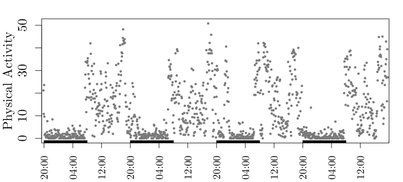
Figure 1.1: ime series for a healthy individual. Rectangles on the time axis correspond to periods from 20.00 to 8.00.

We conduct Bayesian inference using a ikelihood model that is a reformulation of any given We utilise the method of Langrock & Zucchini (2011) to embed the generic state duration distribution within a special transition matrix structure that can approximate the underlying ith arbitrary accuracy. This framework is able to incorporate the extra flexibility of explicitly modelling the state dwell distribution provided by a without renouncing the computational tractability, theoretical understanding, and the multitudes of methodological advancements that are available when using an To the best of our knowledge, such a modeling approach has only previously been treated from a non-Bayesian perspective in the literature, where parameters are estimated either by direct numerical likelihood maximization ( or applying the expectation-maximization ( algorithm.

The main practical advantages of a fully Bayesian framework for nference are that the regularisation and uncertainty quantification provided by the prior and posterior distributions can be readily incorporated into improved mechanisms for prediction and model selection. In particular, selecting the well distribution in a data-driven manner and performing predictive inference for future state dwell times.

However, the posterior distribution is rarely available in closed form and the computational burden of approximating the posterior, often by sampling (see e.g. Gelfand & Smith 1990), is considered a major drawback of the Bayesian approach. In particular, evaluating the likelihood in s already computationally burdensome (Guédon 2003), yielding implementations that are often prohibitively slow. This further motivates the use of the likelihood approximation of Langrock & Zucchini (2011) within a Bayesian framework. Here, we combine their approach with the stan probabilistic programming language (Carpenter et al. 2016), further accelerating the likelihood evaluations by proposing a sparse matrix implementation and leveraging stan’s compatibility with bridge sampling (Meng & Wong 1996, Meng & Schilling 2002, Gronau et al. 2020) to facilitate Bayesian model selection. We provide examples to illustrate the statistical advantages of our Bayesian implementation in terms of prior regularization, forecasting, and model selection and further illustrate that the combination of our approaches can make such inferences computationally feasible (for example, by reducing the time for inference from more than three days to less than two hours), whilst incurring negligible statistical error.

The rest of this article is organized as follows. In Section 2.1, we provide a brief introduction to nd Section 2.2 reviews the ikelihood approximation of Langrock & Zucchini (2011). Section 3 presents our Bayesian framework and inference approach. Using several simulation studies, Section 4 investigates the performance of our proposed procedure when compared with the implementation of Langrock & Zucchini (2011). Section 5 evaluates the trade-off between computational efficiency and statistical accuracy of our method and proposes an approach to investigate the quality of the likelihood approximation for given data. Section 6 illustrates the use of our method to analyze telemetric activity data, and we further investigate the inclusion of spectral information within the emission density in Section LABEL:sec:harmonic_emissions. The stan files (and R utilities) that were used to implement our experiments are available at https://github.com/Beniamino92/BayesianApproxHSMM. The probabilistic programming framework associated with stan makes it easy for practitioners to consider further dwell/emission distributions to the ones considered in this paper. Users need only change the corresponding function in our stan files.

2 Modeling Approach

2.1 Overview of Hidden Markov and Semi-Markov Models

We now provide a brief introduction to the standard nd pproaches before considering the special structure of the transition matrix presented by Zucchini et al. (2017), which allows the state dwell distribution to be generalized with arbitrary accuracy. or Markov switching processes, have been shown to be appealing models in addressing learning challenges in time series data and have been successfully applied in fields such as speech recognition (Rabiner 1989, Jelinek 1997), digit recognition (Raviv 1967, Rabiner et al. 1989) as well as biological and physiological data (Langrock et al. 2013, Huang et al. 2018, Hadj-Amar et al. 2021). An s a stochastic process model based on an unobserved (hidden) state sequence $\bm{s}=(s_{1},\dots,s_{T})$ that takes discrete values in the set $\{1,\dots,K\}$ and whose transition probabilities follow a Markovian structure. Conditioned on this state sequence, the observations $\bm{y}=(y_{1},\dots,y_{T})$ are assumed to be conditionally independent and generated from a parametric family of probability distributions $f(\bm{\theta}_{j})$, which are often called emission distributions. This generative process can be outlined as

$$\begin{split}s_{\,t}\,|\,s_{\,t-1}&\sim\bm{\gamma}_{s_{\,t-1}}\\ y_{t}\,|\,s_{\,t}\,&\sim\,f\,(\,\bm{\theta}_{s_{\,t}})\qquad t=1,\dots,T,\end{split}$$ (2.1)

where $\bm{\gamma}_{\,j}=(\gamma_{j1},\dots,\gamma_{jK})$ denotes the state-specific vector of transition probabilities, $\gamma_{jk}=p\,(\,s_{t}=k\,|\,s_{t-1}=j)$ with $\sum_{k}\gamma_{jk}=1$, and $p\,(\cdot)$ is a generic notation for probability density or mass function, whichever appropriate. The initial state $s_{0}$ has distribution $\bm{\gamma}_{0}=(\gamma_{01},\dots,\gamma_{0K})$ and $\bm{\theta}_{j}$ represents the vector of emission parameters modelling state $j$. rovide a simple and flexible mathematical framework that can be naturally used for many inference tasks, such as signal extraction, smoothing, filtering and forecasting (see e.g. Zucchini et al. 2017). These appealing features are a result of an extensive theoretical and methodological literature that includes several dynamic programming algorithms for computing the likelihood in a straightforward and inexpensive manner (e.g. forward messages scheme, Rabiner 1989). re also naturally suited for local and global decoding (e.g. Viterbi algorithm, Forney 1973), and the incorporation of trend, seasonality and covariate information in both the observed process and the latent sequence. Although computationally convenient, the Markovian structure of imits their flexibility. In particular, the dwell duration in any state, namely the number of consecutive time points that the Markov chain spends in that state, is implicitly forced to follow a geometric distribution with probability mass function $p_{j}(d)=(1-\gamma_{jj})\,\gamma_{jj}^{\,d-1}$.

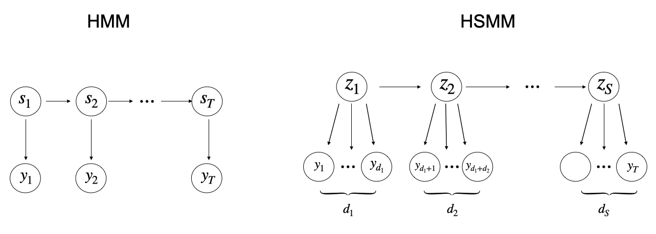
Figure 2.1: Graphical models: (left) here $y_{1},\dots,y_{T}$ are the observations and $s_{1},\dots,s_{T}$ the corresponding hidden state sequence; (right) here $d_{1},\dots,d_{S}$ are the random dwell-times associated with each super state of the Markov chain $z_{1},\dots,z_{S}$ where no self-transitions are allowed.

A more flexible framework can be formulated using where the generative process of an s augmented by introducing an explicit, state specific, form for the dwell time (Guédon 2003, Johnson & Willsky 2013). The state stays unchanged until the duration terminates, at which point there is a Markov transition to a new regime. As depicted in Figure 2.1, the super-states $\bm{z}=(z_{1},\dots,z_{S})$ are generated from a Markov chain prohibiting self-transitions wherein each super-state $z_{s}$ is associated with a dwell time $d_{s}$ and a random segment of observations $\bm{y}_{s}=(y_{t_{s}^{1}},\dots,y_{t_{s}^{2}})$, where $t_{s}^{1}=1+\sum_{r<s}d_{r}$ and $t_{s}^{2}=t_{s}^{1}+d_{s}-1$ represent the first and last index of segment $s$, and $S$ is the (random) number of segments. Here, $d_{s}$ represents the length of the dwell duration of $z_{s}$. The generative mechanism of an an be summarized as

$$\begin{split}z_{\,s}\,|\,z_{\,s-1}&\sim\bm{\pi}_{\,z_{\,s-1}}\\ d_{s}\,|\,z_{s}\,&\sim g\,(\,\bm{\lambda}_{\,z_{s}})\\ \bm{y}_{s}\,|\,z_{\,s}\,&\sim\,f\,(\,\bm{\theta}_{z_{\,s}})\qquad s=1,\dots,S,\end{split}$$ (2.2)

where $\bm{\pi}_{\,j}=(\pi_{j1},\dots,\pi_{jK})$ are state-specific transition probabilities in which $\pi_{jk}=p\,(\,z_{t}=k\,|\,z_{t-1}=j,\,z_{t}\neq j)$ for $j,k=1,\dots,K$. Note that $\pi_{jj}=0$, since self transitions are prohibited. We assume that the initial state has distribution $\bm{\pi}_{0}=(\pi_{01},\dots,\pi_{0K})$, namely $\bm{z}_{0}\sim\bm{\pi}_{0}$. Here, $g$ denotes a family of dwell distributions parameterized by some state-specific duration parameters $\bm{\lambda}_{j}$, which could be either a scalar (e.g. rate of a Poisson distribution), or a vector (e.g. rate and dispersion parameters for negative binomial durations). Unfortunately, this increased flexibility in modeling the state duration has the cost of substantially increasing the computational burden of computing the likelihood: the message-passing procedure for equires $\mathcal{O}\,(T^{2}K+TK^{2})$ basic computations for a time series of length $T$ and number of states $K$, whereas the corresponding forward-backward algorithm for equires only $\mathcal{O}\,(TK^{2})$.

2.2 Approximations to Hidden Semi-Markov Models

In this section we introduce the ikelihood approximation of Langrock & Zucchini (2011). Let us consider an n which $\bm{y}^{\star}=(y^{\star}_{1},\dots,y^{\star}_{T}$) represents the observed process and $\bm{z}^{\star}=(z^{\star}_{1},...,z^{\star}_{T})$ denotes the latent discrete-valued sequence of a Markov chain with states $\{1,2,\dots,\bar{A}\}$, where $\bar{A}=\sum_{i=1}^{K}a_{i}$, and $a_{1},\dots,a_{K}$ are arbitrarily fixed positive integers. Let us define state aggregates $A_{j}$ as

$$A_{j}=\Bigg{\{}\,a:\sum_{i=0}^{j-1}a_{i}<a\leq\sum_{i=0}^{j}a_{i}\,\Bigg{\}},\quad j=1,\dots,K,$$ (2.3)

where $a_{0}=0$, and each state corresponding to $A_{j}$ is associated with the same emission distribution $f(\,\bm{\theta}_{j})$ in the ormulation of Eq. (2.2), namely $y^{\star}_{t}\,\big{|}\,z^{\star}_{\,t}\in A_{j}\sim f\,(\bm{\theta}_{j}).$ The probabilistic rules governing the transitions between states $\bm{z}^{\star}$ are described via the matrix $\bm{\Phi}=\big{\{}\phi_{il}\big{\}}$, where $\phi_{il}=p\,(\,z^{\star}_{\,t}=l\,|\,z^{\star}_{\,t-1}=i\,)$, for $i,l=1,\dots,\bar{A}$. This matrix has the following structure

$$\bm{\Phi}=\begin{bmatrix}\bm{\Phi}_{11}&\dots&\bm{\Phi}_{1K}\\ \vdots&\ddots&\vdots\\ \bm{\Phi}_{K1}&\dots&\bm{\Phi}_{KK}\end{bmatrix},$$ (2.4)

where the sub-matrices $\bm{\Phi}_{jj}$ along the main diagonal, of dimension $a_{j}\times a_{j}$, are defined for $a_{j}\geq 2$, as

$$\bm{\Phi}_{jj}=\begin{bmatrix}0&1-h_{j}\,(1)&0&\dots&0\\ \vdots&0&\ddots&&\vdots\\ &\vdots&&&0\\ 0&0&\dots&0&1-h_{j}\,(a_{j}-1)\\ 0&0&\dots&0&1-h_{j}\,(a_{j})\end{bmatrix},$$ (2.5)

and $\bm{\Phi}_{jj}=1-h_{j}(1)$, for $a_{j}=1$. The $a_{j}\times a_{k}$ off-diagonal matrices $\bm{\Phi}_{jk}$ are given by

$$\bm{\Phi}_{jk}=\begin{bmatrix}\pi_{jk}\,h_{j}\,(1)&0&\dots&0\\ \pi_{jk}\,h_{j}\,(2)&0&\dots&0\\ \vdots&&&\\ \pi_{jk}\,h_{j}\,(a_{j})&0&\dots&0\end{bmatrix}$$ (2.6)

where in the case that $a_{j}=1$ only the first column is included. Here, $\pi_{jk}$ are the transition probabilities of an s in Eq. (2.2), and the hazard rates $h_{j}\,(r)$ are specified for $r\in\mathbb{N}_{>0}$ as

$$h_{j}\,(r)=\dfrac{p\,(\,d_{j}=r\,|\,\bm{\lambda}_{j})}{p\,(\,d_{j}\geq r\,|\,\bm{\lambda}_{j})},\quad\text{if}\,\,p\,(\,d_{j}\geq r-1\,|\,\bm{\lambda}_{j})<1,$$ (2.7)

and 1 otherwise, where $p\,(\,d_{j}=r\,|\,\bm{\lambda}_{j})$ denotes the probability mass function of the dwell distribution $g\,(\bm{\lambda}_{j})$ for state $j$. This structure for the matrix $\bm{\Phi}$ implies that transitions within state aggregate $A_{j}$ are determined by diagonal matrices $\bm{\Phi}_{jj}$, while transitions between state aggregates $A_{j}$ and $A_{k}$ are controlled by off-diagonal matrices $\bm{\Phi}_{jk}$. Additionally, a transition from $A_{j}$ to $A_{k}$ must enter $A_{k}$ in $\min(A_{k})$. Langrock & Zucchini (2011) showed that this choice of $\bm{\Phi}$ allows for the representation of any duration distribution, and yields an hat is, at least approximately, a reformulation of the underlying In summary, the distribution of $\bm{y}$ (generated from an underlying can be approximated by that of $\bm{y}^{\star}$ (modelled using $\bm{\Phi}$), and this approximation can be designed to be arbitrarily accurate by choosing $a_{j}$ adequately large. In fact, the representation of the dwell distribution through $\bm{\Phi}$ differs from the true distribution, namely the one in the ormulation of Eq. (2.2), only for values larger than $a_{j}$, i.e., in the right tail.

3 Bayesian Inference

Bayesian inference for as long been plagued by the computational demands of evaluating its likelihood. In this section we use the ikelihood approximation of Langrock & Zucchini (2011) to facilitate efficient Bayesian inference for Extending the model introduced in Section 2.2 to the Bayesian paradigm requires placing priors on the model parameters $\bm{\eta}=\big{\{}\,(\bm{\pi}_{j},\,\bm{\lambda}_{j},\,\bm{\theta}_{j})\,\big{\}}_{j=1}^{\,K}$. The generative process of our Bayesian model can be summarized by

$$\begin{split}\bm{\pi}_{j}&\sim\text{Dir}\,(\bm{\alpha}_{0}),\qquad(\bm{\theta}_{j},\bm{\lambda}_{j})\sim H\times G,\qquad j=1,\dots,K,\\ z^{\star}_{\,t}\,|\,z^{\star}_{\,t-1}&\sim\bm{\phi}_{\,z^{\star}_{\,t-1}}\\ \bm{y}^{\star}_{t}\,|\,z^{\star}_{\,t}\in A_{j}\,&\sim\,f\,(\,\bm{\theta}_{j})\,\hskip 130.88284ptt=1,\dots,T,\end{split}$$ (3.1)

where Dir$(\cdot)$ denotes the Dirichlet distribution over a $(K-2)$ dimensional simplex (since the probability of self transition is forced to be zero) and $\bm{\alpha}_{0}$ is a vector of positive reals. Here, $H$ and $G$ represent the priors over emission and duration parameters, respectively, and $\bm{\phi}_{i}$ denotes the $i^{th}$ row of the matrix $\bm{\Phi}$. A graphical model representing the probabilistic structure of our approach is shown in Figure 3.1, where we remark that the entries of the transition matrix $\bm{\Phi}$ are entirely determined by the transition probabilities of the Markov chain $\bm{\pi}_{j}$ and the values of the durations $p\,(\,d_{j}=r\,|\,\bm{\lambda}_{j})$.

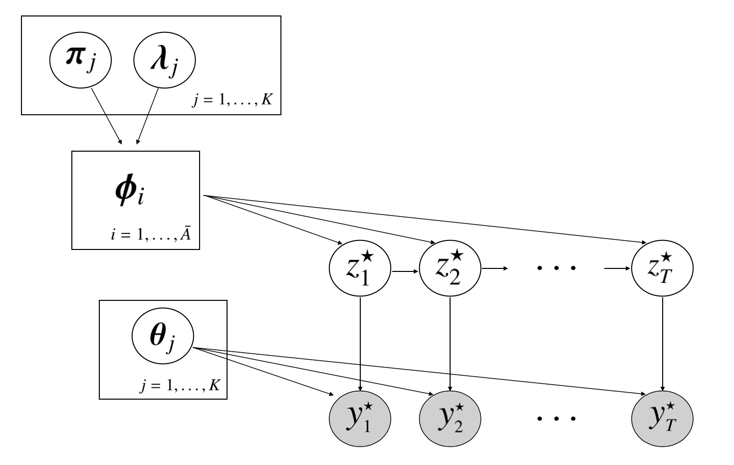
Figure 3.1: A graphical model for Eq. (3.1). Transition probabilities $\bm{\phi}_{j}$ are solely determined by $\bm{\pi}_{j}$ and $p\,(\,d_{j}=r\,|\,\bm{\lambda}_{j})$, and thus they are not considered as random variables themselves.

The posterior distribution for $\bm{\eta}$ has the following factorisation.

$$p\,(\,\bm{\eta}\,|\,\bm{y})\propto\mathscr{L}\,(\bm{y}\,|\,\bm{\eta})\,\times\,\bigg{[}\,\prod_{j=1}^{K}\,p\,(\bm{\pi}_{j})\,\times\,p\,(\bm{\lambda}_{j})\,\times\,p\,(\bm{\theta}_{j})\,\bigg{]}\,,$$ (3.2)

where $\mathscr{L}\,(\,\cdot\,)$ denotes the likelihood of the model, $p\,(\bm{\pi}_{j})$ is the density of the Dirichlet prior for transitions probabilities (Eq. 2.2), and $p\,(\bm{\lambda}_{j})$ and $p\,(\bm{\theta}_{j})$ represent the prior densities for dwell and emission parameters, respectively. Since we have formulated an we can employ well-known techniques that are available to compute the likelihood, and in particular we can express it using the following matrix multiplication (see e.g. Zucchini et al. 2017)

$$\mathscr{L}\,(\bm{y}\,|\bm{\eta})=\bm{\pi}_{0}^{\,\star\,^{\prime}}\,\bm{P}\,(y_{1})\,\bm{\Phi}\,\bm{P}\,(y_{2})\,\bm{\Phi}\,\cdots\,\bm{\Phi}\,\bm{P}\,(y_{T-1})\,\bm{\Phi}\,\bm{P}\,(y_{T})\,\mathbf{1},$$ (3.3)

where the diagonal matrix $\bm{P}\,(\,y\,)$ of dimension $\bar{A}\times\bar{A}$ is defined as

$$\bm{P}\,(\,y\,)=\text{diag}\,\big{\{}\,\underbrace{p\,(y\,|\,\bm{\theta}_{1}),\,\dots,\,p\,(y\,|\,\bm{\theta}_{1})}_{a_{1}\,\,\text{times}},\,\dots,\,\underbrace{p\,(y\,|\,\bm{\theta}_{K})\dots p\,(y\,|\,\bm{\theta}_{K})}_{a_{K}\,\,\text{times}}\big{\}},$$ (3.4)

and $p\,(y\,|\,\bm{\theta}_{j})$ is the probability density of the emission distribution $f\,(\,\bm{\theta}_{j})$. Here, $\mathbf{1}$ denotes an $\bar{A}$-dimensional column vector with all entries equal to one and $\bm{\pi}_{0}^{\,\star}$ represents the initial distribution for the state aggregates. Note that if we assume that the underlying Markov chain is stationary, $\bm{\pi}_{0}^{\,\star}$ is solely determined by the transition probabilities $\bm{\Phi}$, i.e. $\bm{\pi}_{0}^{\,\star}\,=(\bm{I}-\bm{\Phi}+\bm{U})^{\,-1}\,\mathbf{1}$, where $\bm{I}$ is the identity matrix and $\bm{U}$ is a square matrix of ones. Alternatively, it is possible to start from a specified state, namely assuming that $\bm{\pi}_{0}^{\,\star}$ is an appropriate unit vector, e.g. $(1,0,\dots,0)$, as suggested by Leroux & Puterman (1992). We finally note that computation of the likelihood in Eq. (3.3) is often subject to numerical underflow and hence its practical implementation usually require appropriate scaling (Zucchini et al. 2017).

While a fully Bayesian framework is desirable for its ability to provide coherent uncertainty quantification for parameter values, a perceived drawback of this approach compared with a frequentist analogue is the increased computation required for estimation. Bayesian posterior distributions are only available in closed form under the very restrictive setting when the likelihood and prior are conjugate. Unfortunately, the model outlined in Section 2.2 does not admit such a conjugate prior form and as a result the corresponding posterior (Eq. 3.2) is not analytically tractable. However, numerical methods such as Markov Chain Monte Carlo ( can be employed to sample from this intractable posterior. The last twenty years have seen an explosion of research into ethods and more recently approaches scaling them to high dimensional parameter spaces. The next section outlines one such black box implementation that is used to sample from the posterior in Eq. (3.2).

3.1 Hamiltonian Monte Carlo, No-U-Turn Sampler and Stan Modelling Language

One particularly successful posterior sampling algorithm is Hamiltonian Monte Carlo ( Duane et al. 1987), where we refer the reader to Neal et al. (2011) for an excellent introduction. ugments the parameter space with a ‘momentum variable’ and uses Hamiltonian dynamics to propose new samples. The gradient information contained within the Hamiltonian dynamics allows o produce proposals that can traverse high dimensional spaces more efficiently than standard random walk lgorithms. However, the performance of amplers is dependent on the tuning of the leapfrog discretisation of the Hamiltonian dynamics. The No-U-Turn Sampler ( (Hoffman & Gelman 2014) circumvents this burden. ses the Hamiltonian dynamics to construct trajectories that move away from the current value of the sampler until they make a ‘U-Turn’ and start coming back, thus maximising the trajectory distance. An iterative algorithm allows the trajectories to be constructed both forwards and backwards in time, preserving time reversibility. Combined with a stochastic optimisation of the step size, s able to conduct efficient sampling without any hand-tuning.

The stan modelling language (Carpenter et al. 2016) provides a probabilistic programming environment facilitating the easy implementation of The user needs only define the three components of their model: (i) the inputs to their sampler, e.g. data and prior hyperparameters; (ii) the outputs, e.g. parameters of interest; (iii) the computation required to calculate the unnormalized posterior. Following this, stan uses automatic differentiation (Griewank & Walther 2008) to produce fast and accurate samples from the target posterior. stan’s easy-to-use interface and lack of required tuning have seen it implemented in many areas of statistical science. As well as using o automatically tune the sampler, stan is equipped with a variety of warnings and tools to help users diagnose the performance of their sampler. For example, convergence of all quantities of interest is monitored in an automated fashion by comparing variation between and within simulated samples initialized at over-dispersed starting values (Gelman et al. 2017). Additionally, the structure of the transition matrix $\bm{\Phi}$ allows us to take advantage of stan’s sparse matrix implementation to achieve vast computational improvements. Although $\bm{\Phi}$ has dimension $\bar{A}\times\bar{A}$, each row has at most $K$ non-zero terms (representing within state transitions to the next state aggregate or between state transitions), and as a result only a proportion $(K/\bar{A})$ of the elements of $\bm{\Phi}$ is non-zero. Hence, for large values of the dwell approximation thresholds $\bm{a}$, the matrix $\bm{\Phi}$ exhibits considerable sparsity. The stan modelling language implements compressed row storage sparse matrix representation and multiplication, which provides considerable speed up when the sparsity is greater than 90% (Stan Development Team 2018, Ch. 6). In our applied scenario we consider dwell-approximation thresholds as big as $\bm{a}=(250,50,50)$ with sparsity of greater than 99% allowing us to take considerable advantage of this formulation. Finally, we note that our proposed Bayesian approach may suffer from label switching (Stephens 2000) since the likelihood is invariant under permutations of the labels of the hidden states. However, this issue is easily addressed using order constraints provided by stan. This strategy worked well in the simulations and applications presented in the paper, without introducing any noticeable bias in the results.

3.2 Bridge Sampling Estimation of the Marginal Likelihood

The Bayesian paradigm provides a natural framework for selecting between competing models by means of the marginal likelihood, i.e.

$$p\,(\bm{y})=\int\mathscr{L}\,(\bm{y}\,|\,\bm{\eta})\,p\,(\bm{\eta})\,d\bm{\eta}.$$ (3.5)

The ratio of marginal likelihoods from two different models, often called the Bayes factor (Kass & Raftery 1995), can be thought of as the weight of evidence in favor of a model against a competing one. The marginal likelihood in Eq. 3.5 corresponds to the normalizer of the posterior $p\,(\bm{\eta}\,|\,\bm{y})$ (Eq. 3.2) and is generally the component that makes the posterior analytically intractable. lgorithms, such as the stan’s implementation of ntroduced above, allow for sampling from the unnormalized posterior, but further work is required to estimate the normalizing constant. Bridge sampling (Meng & Wong 1996, Meng & Schilling 2002) provides a general procedure for estimating these marginal likelihoods reliably. While standard Monte Carlo ( estimates draw samples from a single distribution, bridge sampling formulates an estimate of the marginal likelihood using the ratio of two stimates drawn from different distributions: one being the posterior (which has already been sampled from) and the other being an appropriately chosen proposal distribution $q\,(\bm{\eta})$. The bridge sampling estimate of the marginal likelihood is then given by

$$p\,(\bm{y})=\frac{\mathbb{E}_{\,q(\bm{\eta})}\left[h(\bm{\eta})\,\mathscr{L}\,(\bm{y}\,|\,\bm{\eta})\,p\,(\bm{\eta})\,\right]}{\mathbb{E}_{\,p(\bm{\eta}|\bm{y})}\left[h(\bm{\eta})\,q(\bm{\eta})\right]}\approx\frac{\frac{1}{n_{2}}\sum_{j=1}^{n_{2}}h(\bm{\tilde{\eta}}^{\,(j)})\,\mathscr{L}\,(\bm{y}\,|\,\bm{\tilde{\eta}}^{\,(j)})\,p\,(\bm{\tilde{\eta}}^{\,(j)})}{\frac{1}{n_{1}}\sum_{i=1}^{n_{1}}h\,(\bm{\overline{\eta}}^{\,(i)})\,q(\bm{\overline{\eta}}^{\,(i)})},$$

where $h(\bm{\eta})$ is an appropriately selected bridge function and $p(\bm{\eta})$ denotes the joint prior distribution. Here, $\{\bm{\overline{\eta}}^{\,(1)},\ldots,\bm{\overline{\eta}}^{\,(n_{1})}\}$ and $\{\bm{\tilde{\eta}}^{\,(1)},\ldots,\bm{\tilde{\eta}}^{\,(n_{2})}\}$ represent $n_{1}$ and $n_{2}$ samples drawn from the posterior $p\,(\bm{\eta}\,|\,\bm{y})$ and the proposal distribution $q(\bm{\eta})$, respectively. This estimator can be implemented in R using the package bridgesampling (Gronau et al. 2020), whose compatibility with stan makes it particularly straightforward to estimate the marginal likelihood directly from a stan output. This package implements the method of Meng & Wong (1996) to choose the optimal bridge function minimising the estimator mean-squared error and constructs a multivariate normal proposal distribution whose mean and variance match those of the sample from the posterior.

3.3 Comparable Dwell Priors

Model selection based on marginal likelihoods can be very sensitive to prior specifications. In fact, Bayes factors are only defined when the marginal likelihood under each competing model is proper (Robert 2007, Gelman et al. 2013). As a result, it is important to include any available prior information into the Bayesian modelling in order to use these quantities in a credible manner. Reliably characterising the prior for the dwell distributions is particularly important for the experiments considered in Section 6, since we use Bayesian marginal likelihoods to select between the dwell distributions associated with nd For instance, if we believe that the length of sleep for an average person is between 7 and 8 hours we would choose a prior that reflects those beliefs in all competing models. However, we need to ensure that we encode this information in comparable priors in order to perform ‘fair’ Bayes factor selection amongst a set of dwell-distributions. Our aim is to infer which dwell distribution, and not which prior specification, is most appropriate for the data at hand.

For example, suppose we consider selecting between geometric (i.e. an , negative binomial or Poisson distributions (i.e. an , to model the dwell durations of our data. While a Poisson random variable, shifted away from zero to consider strictly positive dwells, has its mean $\lambda_{j}+1$ and variance $\lambda_{j}$ described by the same parameter $\lambda_{j}$, the negative binomial allows for further modelling of the precision through an additional factor $\rho_{j}$. In both negative binomial and Poisson the parameters $\lambda_{j}$ are usually assigned a prior $\lambda_{j}\sim\text{Gamma}\,(a_{0j},b_{0j})$ with mean $\mathbb{E}\left[\lambda_{j}\right]=a_{0j}/b_{0j}$ and variance $\textrm{Var}\left[\lambda_{j}\right]=a_{0j}/b_{0j}^{2}$. In order to develop an interpretable comparison of all competing models, we parameterize the geometric dwell distribution associated with state $j$ in the standard Eq. 2.1) as also being characterized by the mean dwell length $\tau_{j}=1/(1-\gamma_{jj})$, where the geometric is also shifted to only consider strictly positive support and $\gamma_{jj}$ represents the probability of self-transition. Under a Dirichlet prior for the state-specific vector of transition probabilities $\bm{\gamma}_{j}=(\gamma_{j1},\ldots,\gamma_{jK})\sim\text{Dirichlet}(\bm{v}_{j})$, with $\bm{v}_{j}=(v_{j1},\ldots,v_{jK})$ and $\beta_{j}=\sum_{i\neq j}v_{ji}$, the mean and variance of the prior mean dwell under an re given by

$$\mathbb{E}\left[\tau_{j}\right]=\frac{v_{jj}+\beta_{j}-1}{\beta_{j}-1}\textrm{ and }\textrm{Var}\left[\tau_{j}\right]=\frac{(v_{jj}+\beta_{j}-1)(v_{jj}+\beta_{j}-2)}{(\beta_{j}-1)(\beta_{j}-2)}-\left(\frac{v_{jj}+\beta_{j}-1}{\beta_{j}-1}\right)^{2}$$

for $\beta_{j}>2$ (the derivation of this result is provided in the Supplementary Material).

We therefore argue that a comparable prior specification requires hyper-parameters $\{a_{0j},b_{0j}\}_{j=1}^{K}$ and $\{\bm{v}_{j}\}_{j=1}^{K}$ be chosen in a way that satisfy $\mathbb{E}\left[\tau_{j}\right]=\mathbb{E}[\lambda_{j}+1]$ and $\textrm{Var}\left[\tau_{j}\right]=\textrm{Var}\left[\lambda_{j}+1\right]$, ensuring the dwell distribution in each state has the same prior mean and variance across models. The prior mean can be interpreted as a best a priori guess for the average dwell time in each state, and the variance reflects the confidence in this prior belief. In addition, since the negative binomial distribution is further parameterized by a dispersion parameter $\rho_{j}$, we center our prior belief at $\rho_{j}=1$, which is the value that recovers geometric dwell durations (namely an when $\lambda_{j}=\gamma_{jj}/(1-\gamma_{jj})$. Between state transition probabilities, i.e. the non-diagonal entries of the transition matrix, as well as the emission parameters, are shared between the nd and thus we may place a prior specification on these parameters that is common across all models.

4 A Comparison with Langrock and Zucchini (2011)

This section presents several simulation studies. Firstly, we show that our Bayesian implementation provides similar point estimates as the methodology of Langrock & Zucchini (2011), serving as a “sanity check”. We then proceed to illustrate the benefits adopting a Bayesian paradigm can bring to odelling.

4.1 Parameter Estimation

For our first example, we simulated $T=200$ data points from a three-state Eq. 2.2). Conditional on each state $j$, the observations are generated from a $\text{Normal}\left(\mu_{j},\sigma_{j}^{2}\right)$, and the dwell durations are Poisson$(\lambda_{j}$) distributed. We consider relatively large values for $\lambda_{j}$ in order to evaluate the quality of the pproximation provided by Eq. (3.1). The full specification is provided in Table 4.1 and a realization of this model is shown in Figure 4.1 (a, top). The dwell approximation thresholds $\bm{a}$ are set equal to $(30,30,30)$ and we placed a Gamma$(0.01,0.01)$ prior on the Poisson rates $\lambda_{j}$. The transition probabilities $\bm{\pi}_{j}$ are distributed as $\text{Dirichlet}(1,1)$ and the priors for the Gaussian emissions are given as $\text{Normal}(0,10^{2})$ and $\text{Inverse-Gamma}(2,0.5)$ for locations $\mu_{j}$ and scale $\sigma^{\,2}_{j}\,$, respectively. Overall, this prior specification is considered weakly informative (Gelman et al. 2013, 2017).

Table 4.1 shows estimation results for our proposed Bayesian methodology as well as the analogous frequentist approach ( of Langrock & Zucchini (2011), which will be referred to as LZ-2011. Figure 4.1 (a) displays: (top) a graphical posterior predictive check consisting of the observations alongside 100 draws from the estimated posterior predictive (Gelman et al. 2013); (bottom) the most likely hidden state sequence, i.e. $\operatorname*{arg\,max}_{\bm{z}}p\,(\,\bm{z}\,|\,\bm{y},\,\bm{\eta}\,)$, which is estimated via the Viterbi algorithm (see e.g. Zucchini et al. 2017) using plug-in Bayes estimates of the model parameters; In order to assess the goodness of fit of the model, we also verified normality of the pseudo-residual (see Supplementary Material).

	True	LZ-2011	Proposed			True	LZ-2011	Proposed			True	LZ-2011	Proposed
$\mu_{1}$	5	4.96	4.95 (4.66–5.24)		$\sigma_{3}$	1	1.01	1.08 (0.90–1.20)		$\pi_{13}$	0.70	0.50	0.5 (0.13–0.87)
$\mu_{2}$	14	14.02	14.02 (13.67–14.37)		$\lambda_{1}$	20	23.47	23.36 (17.03–30.57)		$\pi_{21}$	0.20	0.00	0.20 (0.01–0.53)
$\mu_{3}$	30	30.19	30.18 (29.98–30.38)		$\lambda_{2}$	30	27.22	27.05 (22.43–32.19)		$\pi_{23}$	0.80	1.00	0.80 (0.47–0.99)
$\sigma_{1}$	1	1.09	1.15 (0.95–1.40)		$\lambda_{3}$	20	19.98	20.00 (15.93–24.46)		$\pi_{31}$	0.10	0.33	0.40 (0.10–0.76)
$\sigma_{2}$	2	1.90	1.95 (1.73–2.22)		$\pi_{12}$	0.30	0.50	0.50 (0.13–0.87)		$\pi_{32}$	0.90	0.67	0.60 (0.24–0.90)

Table 4.1: Illustrative Example. True model parameterization and corresponding estimates obtained via the EM algorithm and our proposed Bayesian approach. For the latter, we also report $95\%$ credible intervals estimated from the posterior sample.

In general, both methods satisfactorily retrieve the correct pre-fixed duration and emission parameters and the posterior predictive checks indicate that our posterior sampler is performing adequately. The implementation of Langrock & Zucchini (2011) suffers from a lack of regularisation, for example in the estimation of $\pi_{21}$ as 0, and is not currently available with an automatic method to quantify parameter uncertainty. While augmenting the approach of Langrock & Zucchini (2011) by adding regularisation penalties to parameters and producing confidence measures such as standard errors and bootstrap estimates is possible, such features are automatic to our Bayesian adaptation. Further, such an approach allows this uncertainty to be incorporated into methods for prediction and model selection making the Bayesian paradigm appealing for odelling.

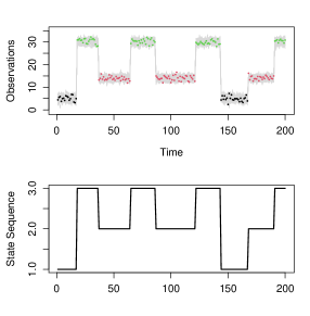
(a)

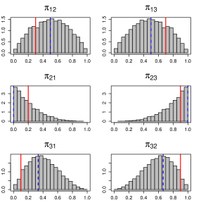
(b)

Figure 4.1: (a, top) a realization (dots) of a three-state ith Gaussian emissions and Poisson durations, where different colors correspond to (true) different latent states. Grey lines represent 100 samples drawn from the estimated posterior predictive distribution. (a, bottom) Most likely hidden state sequence estimated via the Viterbi algorithm; (b) estimated posterior distribution of the transition probabilities $\pi_{jk}$, where vertical solid red and blue dotted lines represent true values and EM estimates, respectively.

4.2 Forecasting

A key feature of s their ability to be able to capture and forecast when and for how long the model will be in a given state. We compare the forecasting properties of the method presented by Langrock & Zucchini (2011) and our proposed Bayesian approach. We simulated 20 ‘un-seen’ time series, $\tilde{\bm{y}}=(\tilde{y}_{\,1},\,\ldots,\tilde{y}_{H})$, where $\tilde{y}_{\,h}=y_{\,T+h},\hskip 2.84544pth=1,\dots,H$ and $H=100,300,500$ denotes the forecast horizon, from the model as in Table 4.1. We used the logarithmic score (log-score) to measure predictive performances. Let $\hat{\bm{\eta}}$ be the frequentist ( parameter estimate and define the log-score

$$L_{\,\text{freq}}(\tilde{\bm{y}})=\sum_{h=1}^{H}-\log p\,(\tilde{y}_{h}\,|\,\hat{\bm{\eta}}),$$

where $p\,(\tilde{y}_{h}\,|\,\hat{\bm{\eta}})$ denotes the forecast density function (see Supplementary Material for an explicit expression). Our Bayesian framework does not assume a point estimate $\hat{\bm{\eta}}$ but considers instead a posterior distribution $p\,(\bm{\eta}\,|\,\bm{y})$, which is integrated over to produce a predictive density. Given $M$ amples drawn from the posterior, $\left\{\bm{\eta}^{(i)}\right\}_{i=1}^{M}\sim\pi\,(\bm{\eta}\,|\,\bm{y})$, the log-score of the predictive density can be approximated as

$$L_{\,\text{Bayes}}(\tilde{\bm{y}})=\sum_{h=1}^{H}-\log p\,(\tilde{y}_{h}\,|\,\bm{y}) =\sum_{h=1}^{H}-\log\int p\,(\tilde{y}_{h}\,|\,\bm{\eta})\,p\,(\bm{\eta}\,|\,\bm{y})\,d\bm{\eta}$$

$$\approx\sum_{h=1}^{H}-\log\left(\frac{1}{M}\sum_{i=1}^{M}p\,(\tilde{y}_{h}\,|\,\bm{\eta}^{(i)})\right).$$

Figure 4.2 presents box-plots of log-scores for LZ-2011 and our proposed Bayesian approach. It is clear that our Bayesian methodology typically produces a much lower predictive log-score than the frequentist procedure. The approach by Langrock & Zucchini (2011) which uses plug-in estimates for parameters, is known to ‘under-estimate’ the true predictive variance thus yielding large values of the log-score (Jewson et al. 2018). On the other hand, our Bayesian paradigm integrates over the parameters and hence is more accurately able to capture the true forecast distribution. As a result, it produces significantly smaller log-score estimates.

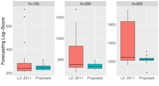
Figure 4.2: Boxplots of log-scores for LZ-2011 (via and our Bayesian methodology, with three different forecast horizons $H=100,300,500$.

4.3 Dwell Distribution Selection

An important consideration is whether to formulate an or to extend the dwell distribution beyond a geometric one (i.e., an . Ideally, the data should be used to drive such a decision. In this section, we compare the frequentist methods for doing so, namely Akaike’s information criterion ( Akaike 1973) and Bayesian information criterion ( Schwarz et al. 1978), with their Bayesian counterpart, namely the marginal likelihood. We choose not to consider other Bayesian inspired information criteria (e.g. Spiegelhalter et al. 2002, Watanabe 2010, Gelman et al. 2014) as our goal here is to compare standard frequentist methods used previously in the literature to conduct model selection for nd [e.g.][]langrock2011hidden, huang2018hidden with the canonical Bayesian analog. Although the performance of Bayesian model selection can be sensitive to the specification of the prior, we gave specific consideration to specifying this with model selection in mind in Section 3.3.

4.3.1 Consistency for Nested Models

A special feature of the negative binomial dwell distribution is that the geometric dwell distribution associated with s nested within it. Taking $\rho=1$ for the negative binomial exactly corresponds to the geometric distribution. An important consideration when selecting between nested models is complexity penalization. For the same data set, the more complicated of two nested models will always achieve a higher in-sample likelihood score than the simpler model. Therefore, in order to achieve consistent model selection among nested models, the extra parameters of the more complex models must be penalized. In this scenario, the := -2 $\mathscr{L}\,(\bm{y}\,|\,\bm{\eta})+2p$ where $p$ denotes the number of parameters included in the model, is known not to provide consistent model selection when the data is generated from the simpler model (see e.g. Fujikoshi 1985). On the other hand, performing model selection using the marginal likelihood can be shown to be consistent (see e.g. O’Hagan & Forster 2004), provided some weak conditions on the prior are satisfied. Therefore, when following a Bayesian paradigm, the correct data generating model is selected with probability one as $T$ tends to infinity. Here we show that under the approximate ikelihood model, Bayesian model selection appears to maintain its desirable properties. We simulated 20 time series from a two-state ith Gaussian emission parameters $\bm{\mu}=(1,4)$ and $\bm{\sigma}^{2}=(1,1.5)$, and diagonal entries of the transition matrix set to $(\gamma_{11},\gamma_{22})=(0.7,0.6)$. To model this data we considered the nd a ith negative binomial durations . For the pproximation, we considered $\bm{a}=(3,3)$, $(5,5)$ and $(10,10)$ in order to investigate how the dwell approximation affects the model selection performance. We use prior distributions that are comparable as explained in Section 3.3, the exact prior specifications are presented in the Supplementary Material. Figure 4.3 (top) displays box-plots of the difference between the model selection criteria (namely marginal likelihood and achieved by the nd the for increasing sample size $T=500,5000,10000$ and values for $\bm{a}$. We negate the uch that maximising both criteria is desirable. Thus, positive values for the difference correspond to correctly selecting the simpler data generating model, i.e. the As the sample size $T$ increases, the marginal likelihood appears to converge to a positive value, and the variance across repeats decreases, indicating consistent selection of the correct model. On the other hand, even for large $T$ there are still occasions when the trongly favours the incorrect, more complicated model. Further, such performance appears consistent across values of $\bm{a}$.

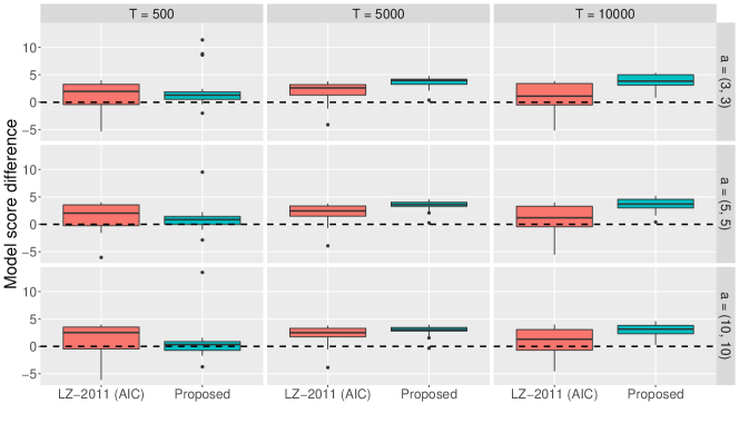
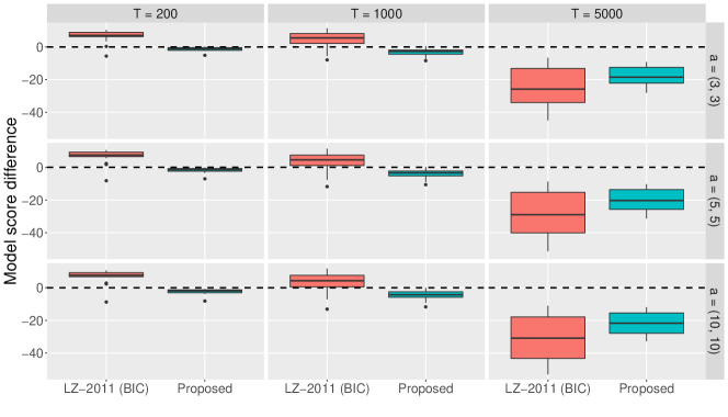
Figure 4.3: nd the marginal likelihood for nested models. (Top) model score differences between a negative binomial duration ith $\bm{a}=(3,3),(5,5)$ and $(10,10)$ and an hen the data is generated from the Positive values of the model score difference correspond to correctly selecting the simpler model. (Bottom) model score differences between a negative binomial duration pproximated by a threshold $\bm{a}=(3,3),(5,5)$ and $(10,10)$ and an hen the data is generated from the Negative values of the model score difference correspond to correctly selecting the more complicated model. Note that here we interpret the difference between the nd the log-marginal likelihood values of two models as quantitatively comparable for model selection decisions, with being greater than or less than 0 corresponding to the selection decision.

4.3.2 Complexity Penalization

Unlike the the $\lx@acro@@@def{\smaller BIC}{\smaller BIC}{\,}{{\smaller BIC}}{{\,}}:=-2\,\mathscr{L}\,(\bm{y}\,|\,\bm{\eta})+p\log T$ penalizes complexity in a manner that depends on the sample size $T$. This is termed ‘Bayesian’ because it corresponds to the Laplace approximation of the marginal likelihood of the data (Konishi & Kitagawa 2008), often interpreted as considering a uniform prior for the model parameters (Bhat & Kumar 2010, Sodhi & Ehrlich 2010). Though the uniform distribution may be viewed as naturally uninformative, it is well known that using the marginal likelihood assuming an uninformative prior specification can lead to the selection of the simplest model independently of the data (see e.g. Lindley 1957, Jeffreys 1998, Jennison 1997). As a result, while an provide consistent selection of nested models, it can punish extra complexity in an excessive manner. To investigate how the approximate ikelihood model affects this model selection behaviour, we consider data generated from an ith the same formulation as above except that in this scenario the dwell distribution is a negative binomial parameterized by state-specific parameters $\bm{\lambda}=(3.33,2.50)$ and $\bm{\rho}=(2,0.5)$. Note that the data generating as two more parameters than the For the pproximation, we consider $\bm{a}=(3,3)$, $(5,5)$ and $(10,10)$, where the largest of these provides negligible truncation of the right tail of the dwell distribution given the data generating parameters. Figure 4.3 (bottom) shows box-plots of the difference between the model scores (marginal-likelihood and across 20 simulated time series when fitting the nd for increasing sample size $T=200,1000,5000$ and values for $\bm{a}$. We negate the o that the preferred model maximises both criteria. Unlike the experiments described above, the data is now from the less parsimonious pproach and therefore negative values for the difference in score correspond to correctly selecting the more complicated model. For small sample sizes, e.g. $T=200,1000$, the complexity penalty of the ppears to be too large, so that in almost all of the 20 repeat experiments the simple model is incorrectly favored over the correct data generating model, i.e. the On the other hand, the marginal likelihood is able to correctly select the more complicated model across almost all simulations and sample sizes. Although for smaller $\bm{a}$ the pproximation is ‘closer’ to a we still see that the model selection performance is consistent across the different values of $\bm{a}$.

5 Approximation Accuracy and Computational Time

The previous section motivated why the Bayesian paradigm can improve statistical inferences for Next, we investigate the computational feasibility of such an approach and the trade-off between computational efficiency and statistical accuracy achieved by our Bayesian approximate mplementation. In particular, we compare our Bayesian approximate ethod for different values of the threshold $\bm{a}$ with a Bayesian implementation of the exact while also illustrating the computational savings made by our sparse matrix implementation. For the exact the full-forward recursion is used to evaluate the likelihood (see e.g. Guédon 2003 or Economou et al. 2014). In order to provide a fair comparison, we coded the forward recursion outlined in Economou et al. (2014) in stan also. We then compare the computational resources required to sample from the approximate and exact osteriors with the accuracy of the posterior mean parameter estimates with respect to their data generating values. We generate $T=5000$ observations from two different ith Poisson durations (both with $K=5$ states and the same Gaussian emission distributions). For the two different datasets, we consider the following dwell parameters: (i) short dwells, i.e. $\bm{\lambda}=(2,5,8,1,4)$, where the average time spent in each state is fairly small and (ii) one long dwell, i.e. $\bm{\lambda}=(2,5,25,1,4)$, where four states have short average dwell time and one where the average dwell time is much longer. We also consider two approximation thresholds: $\bm{a}_{1}=(10,10,10,10,10)$, namely a fixed approximation threshold for all five states, and $\bm{a}_{2}=(10,10,30,10,10)$, a ‘hybrid’ model where four of the states have short dwell thresholds and one has a longer threshold. The emission parameters were set to $\bm{\mu}=(1,2,3.5,6,10)$ and $\bm{\sigma}^{2}=(1^{2},0.5^{2},0.75^{2},1.5^{2},2.5^{2})$, and we specify priors $\mu_{j}\sim\mathcal{N}(0,10^{2})$, $\sigma^{2}_{j}\sim\mathcal{IG}(2,0.5)$, $\lambda_{j}\sim\mathcal{G}(0.01,0.01)$ and $\gamma_{j}\sim\mathcal{D}(1,\ldots,1)$ for $j=1,\ldots,5$. The results are presented in Table 5. Across both datasets and approximation thresholds, the sparse implementation takes less than half the time of the non-sparse implementation, with the saving greater when the dwell thresholds are larger (and the matrix $\bm{\Phi}$, Eq. (3.4), is sparser). Furthermore, the pproximations are considerably faster than the full mplementation. For the short dwell dataset the full akes close to 3.5 days while the sparse implementations of the pproximation both require less than 2 hours. Similarly, for the one long dwell dataset, the full akes over 4 days to run while again the sparse pproximations require around 2 hours. The quoted Effective Sample Size ( e.g. Gelman et al. 2013) values are calculated using the LaplaceDemons package in R and are averaged across parameters. These show that the f all the generated samples is close to 1000 and thus the time comparisons are indeed fair. Further, we expect the difference to become starker as the number of observations $T$ increases. While, the approximate cales linearly in $T$ and quadratically in $\sum_{j=1}^{K}a_{j}$, the full n the worst case is quadratic in $T$ (Langrock & Zucchini 2011). Lastly, we see that the savings in computation time come at very little cost in statistical accuracy. We measure the statistical accuracy of the vector-valued parameter $\hat{\bm{\theta}}$ to estimate $\bm{\theta}^{\ast}$ using its mean squared error ( $\sum_{j=1}^{K}(\hat{\theta}_{j}-\theta^{\ast}_{j})^{2}$). All methods achieve almost identically alues for the emission parameters $\bm{\mu}$ and $\bm{\sigma}^{2}$. For the short dwell data, the $\bm{a}_{1}$ approximation has slightly higher or $\bm{\lambda}$ while the $\bm{a}_{2}$ approximation performed comparably to the Clearly, increasing the approximation threshold improves statistical accuracy. On the other hand, the one long dwell shows that if the dwell threshold is set too low, as is the case with $\bm{a}_{1}$, large errors in the dwell estimation can be made. However, in this example the higher dwell approximation $\bm{a}_{2}$ once again performs comparably with the full whilst requiring only $2\%$ of the computational time.

Short dwells Time (hours)    $\mu$ $\sigma^{2}$ $\lambda$ Approx: $\bm{a_{1}}$ 2.62 986.50 3.72 $\times 10^{-2}$ 2.88 $\times 10^{-3}$ 0.25 Approx (SPARSE): $\bm{a_{1}}$ 1.30 975.20 3.84 $\times 10^{-2}$ 3.06 $\times 10^{-3}$ 0.26 Approx: $\bm{a_{2}}$ 3.94 961.76 3.84 $\times 10^{-2}$ 3.05 $\times 10^{-3}$ 0.17 Approx: (SPARSE): $\bm{a_{2}}$ 1.78 978.82 3.96 $\times 10^{-2}$ 3.01 $\times 10^{-3}$ 0.18 Exact 81.15 933.28 4.02 $\times 10^{-2}$ 3.24 $\times 10^{-3}$ 0.19 One long dwell Approx: $\bm{a_{1}}$ 3.33 984.51 1.76 $\times 10^{-2}$ 4.68 $\times 10^{-2}$ 128.50 Approx: (SPARSE): $\bm{a_{1}}$ 1.78 981.90 1.73 $\times 10^{-2}$ 4.84 $\times 10^{-2}$ 128.51 Approx: $\bm{a_{2}}$ 5.08 993.89 1.50 $\times 10^{-2}$ 4.84 $\times 10^{-2}$ 1.25 Approx: (SPARSE): $\bm{a_{2}}$ 2.21 983.47 1.51 $\times 10^{-2}$ 4.82 $\times 10^{-2}$ 1.25 Exact 101.35 980.59 1.65 $\times 10^{-2}$ 4.66 $\times 10^{-2}$ 1.12

Table 5.1: Computational time (hours), effective sample size ( and mean squared error ( of posterior mean parameters. The results are reported using the approximate or different dwell approximations $\bm{a}$ (with the corresponding sparse implementation), and the exact mplementation.

5.1 Setting the Dwell Threshold

The results of Section 5 indicate that while vast computational savings are possible using the approximate ikelihood, care must be taken not to set the dwell approximation threshold $\bm{a}$ too low. We propose initialising $\bm{a}$ based on the prior distribution for the dwell times $d_{j}$, $\pi(d_{j})=\int\pi(d_{j};\lambda)\pi(\lambda)d\lambda$. Noting that any dwell time $d_{j}<\bm{a}_{j}$ is not approximated, we recommend initialising $\tilde{\bm{a}}$ such that $d_{j}\leq\tilde{\bm{a}}_{j}$ with high probability for all $j=1,\ldots,K$. Such an initialisation however does not guarantee the accuracy of the odelling, particularly in the absence of informative prior beliefs. We therefore, propose a diagnostic method to check that $\tilde{\bm{a}}$ is not too small. 1. Initialise $\tilde{\bm{a}}$ and conduct inference on the observed data. Record posterior mean parameter estimates $\hat{\bm{\eta}}_{obs}(\tilde{\bm{a}})$ 2. Generate data $\tilde{y}_{gen}$ from an exact ith generating parameters $\hat{\bm{\eta}}_{obs}(\tilde{\bm{a}})$. Note that generation from an exact s easier than inference on its parameters 3. Continuing with $\tilde{\bm{a}}$, conduct inference on the generated data and record posterior mean parameter estimates $\hat{\bm{\eta}}_{gen}(\tilde{\bm{a}})$ 4. Compare dwell distribution parameters $\hat{\lambda}_{obs}(\tilde{\bm{a}})$ and $\hat{\lambda}_{gen}(\tilde{\bm{a}})$ The estimates $\hat{\lambda}_{obs}(\tilde{\bm{a}})$ provide the best guess estimate of the parameters of the nderlying the data for fixed $\tilde{\bm{a}}$. Generating from this exact iven by these estimates allows us to verify the accuracy of the proposed model. If the estimates are not accurate then little confidence can be had that $\hat{\lambda}_{obs}(\tilde{\bm{a}})$ accurately represents the dwell distribution of the underlying If $\hat{\lambda}_{gen}(\tilde{\bm{a}})_{j}$ is not considered a satisfactory estimate of $\hat{\lambda}_{obs}(\tilde{\bm{a}})_{j}$, then $\tilde{\bm{a}}_{j}$ must be increased. Conveniently, this can be done for each state $j$ independently. Further, if $\hat{\lambda}_{gen}(\tilde{\bm{a}})_{j}$ is considered accurate enough, then there is also the possibility to decrease $\tilde{\bm{a}}_{j}$ based on the inferred dwell distribution. Although the above procedure requires the fitting of the model several times, we believe the computational savings of our model when compared with the exact nference demonstrated in Table 5 render this worthwhile. This procedure is implemented to set the dwell-approximation threshold for the physical activity time series analysed in the next section.

6 Telemetric Activity Data

In this section, we return to the physical activity ( time series that Huang et al. (2018) analysed using a frequentist We seek to conduct a similar study but within a Bayesian framework and consider the extra flexibility afforded by our proposed methodology to investigate departures from the Further, in Section LABEL:sec:harmonic_emissions we consider the inclusion of spectral information within the nd mission densities. We consider three-state with Poisson$\,(\lambda_{j})$ and Neg-Binomial$\,(\lambda_{j},\rho_{j})$ dwell durations, shifted to have strictly non-negative support and approximated via thresholds $\bm{a}_{P}=(160,40,25)$ and $\bm{a}_{NB}=(250,50,50)$ respectively. These are fitted to the square root of the ime series shown in Figure 1.1, wherein we assume that transformed observations are generated from Normal$(\,\mu_{j},\sigma_{j}^{\,2})$ distributions, as in Huang et al. (2018). We specified $K=3$ states, in agreement with findings of Migueles et al. (2017) and Huang et al. (2018), where they collected results from more than forty experiments on ime series. In their studies, for each individual the lowest level of activity corresponds to the sleeping period, which usually happens during the night, while the other two phases are mostly associated with movements happening in the daytime. Henceforth, these different telemetric activities are represented as inactive (, moderately active ( and highly active ( states. The setting of $\bm{a}$ followed the iterative process outlined in Section 5.1, initialising $\tilde{a}_{j}$ giving prior probability of 0.9 that $d_{j}<a_{j}$. This choice also reflects a trade-off between accurately capturing the states with which we have considerable prior information, i.e. whilst improving the computational efficiency of the other states over a standard ormulation. We assume that the night rest period of a healthy individual is generally between 7 and 8 hours. The parameter of the dwell duration of the tate, $\lambda_{\,\lx@acro@@@def{\smaller IA}{\smaller IA}{}{{\smaller IA}}{{}}}$, is hence assigned a Gamma prior with hyperparameters that reflect mean 90 (i.e. $7.5\times 12$) and variance 36 (i.e. $[0.5\times 12]^{2}$), the latter was chosen to account for some variability amongst people. Since we do not have significant prior knowledge on how long people spend in the nd tates, we assigned $\lambda_{\,\lx@acro@@@def{\smaller MA}{\smaller MA}{}{{\smaller MA}}{{}}}$ and $\lambda_{\,\lx@acro@@@def{\smaller HA}{\smaller HA}{}{{\smaller HA}}{{}}}$ Gamma priors with mean 24 (i.e. 2 hours) and variance 324 (i.e. $[1.5\times 12]^{2}$) to reflect a higher degree of uncertainty. Transition probabilities from state $\beta^{(0)}$ $\beta^{(1)}$ $\beta^{(2)}$ $\beta^{(0)}$ $\beta^{(1)}$ $\beta^{(2)}$ $\beta^{(0)}$ $\beta^{(1)}$ $\beta^{(2)}$ Gaussian 0.93 (0.88-0.98) - - 3.18 (3.03-3.33) - - 5.38 (5.27-5.51) - - Harmonic 1.36 (1.26-1.46) 0.04 (-0.05-0.13) -0.60 (-0.72- -0.47) 3.32 (2.94-3.65) -0.11 (-0.34-0.13) -0.24 (-0.69-0.17) 5.46 (5.32-5.60) 0.20 (0.07-0.33) -0.23 (-0.61-0.16)

Table 6.2: Telemetric activity data with harmonic emissions. (Top) Log-marginal likelihood for different dwell durations (i.e. Poisson, geometric and negative binomial). Geometric durations are characterized by their mean dwell length $\lambda_{j}=1/(1-\gamma_{jj})$ where $\gamma_{jj}$ represents the probability of self-transition. (Bottom) Parameters of the mean of the Gaussian and harmonic emission distributions under the selected negative binomial dwell distribution. Estimated posterior means of the parameters are reported with a 90% credible intervals estimated from the posterior sample.

Following the selection of the negative binomial dwell distribution for both the standard Gaussian and harmonic emission models, Table 5 (bottom) provides the posterior mean values for the parameters of these emission distributions, along with the 90% credibility intervals provided by the posterior. These results show that even with a global estimate for the periodicity, there are differences between the estimated parameters in each state, supporting the combination of the periodic time-series model with a hidden state model. Furthermore, there are clear differences between the estimated emissions of the harmonic model compared with the estimated Gaussian emissions in the standard model (where $\beta^{(0)}_{j}=\mu_{j}$ and $\beta^{(1)}_{j}$ and $\beta^{(2)}_{j}$ were both 0). In particular, the intercept $\beta^{(0)}_{\,\lx@acro@@@def{\smaller IA}{\smaller IA}{}{{\smaller IA}}{{}}}$ in the tate differs non-negligibly when using the harmonic model instead of the standard Gaussian, as do $\beta^{(2)}_{\,\lx@acro@@@def{\smaller IA}{\smaller IA}{}{{\smaller IA}}{{}}}$ and $\beta^{(1)}_{\,\lx@acro@@@def{\smaller HA}{\smaller HA}{}{{\smaller HA}}{{}}}$, whose 90% credibility intervals do not cover 0. This all supports the selection of the harmonic model over the standard Gaussian emissions.

7 Concluding Summaries

We presented a Bayesian model for analyzing time series data based on an ormulation with the goal of analyzing physical activity data collected from wearable sensing devices. We facilitate the computational feasibility of Bayesian inference for ia the likelihood approximation introduced by Langrock & Zucchini (2011), in which a special structure of the transition matrix is embedded to model the state duration distributions. We utilize the stan modeling language and deploy a sparse matrix formulation to further leverage the efficiency of the approximate likelihood. We showed the advantages of choosing a Bayesian paradigm over its frequentist counterpart in terms of incorporation of prior information, quantification of uncertainty, model selection, and forecasting. We additionally demonstrated the ability of the pproximation to drastically reduce the computational burden of the Bayesian inference (for example reducing the time for inference on $T=5000$ observations from $>3$ days to $<2$ hours), whilst incurring negligible statistical error. The proposed approach allows for the efficient implementation of highly flexible and interpretable models that incorporate available prior information on state durations. An avenue not explored in the current paper is how our model compares to particle filtering methods. For example, a referee suggested that an algorithm sampling the filtering distribution using an adaptation of the sequential Monte Carlo (SMC) sampler of Yildirim et al. (2013) inside one of the two particle lgorithms of Whiteley et al. (2009) could prove competitive for nference. Further work could define, implement and compare such an approach to ours. The analysis of physical activity data demonstrated that our model was able to learn the probabilistic dynamics governing the transitions between different activity patterns during the day as well as characterizing the sleep duration overnight. We were also able to illustrate the flexibility of the proposed model by adding harmonic covariates to the emission distribution, extending further the analysis of Huang et al. (2018). Future work will investigate the further inclusion of covariates into these time series models as well as computationally and statistically efficient approaches for conducting variable selection among these (George & McCulloch 1993, Rossell & Telesca 2017). We will also consider extending our methodology to account for higher-dimensional multivariate time series, where computational tractability is further challenging.

Acknowledgements

The authors would like to thank the Editor, the Referee, the Associate Editor, David Rossell, and Marina Vannucci for their insightful and valuable comments.

Appendix A Supplementary Material

Section A.1 provides the derivations of the mean and variance of the mean dwell time of an Section A.2 and A.3 includes the form of the forecast function and graphs of pseudo residuals that we utilized in our experiments. In Section A.4 we provide further results about our ata application by comparing different predictive distributions of the state durations as well as investigating state classification. Section A.5 illustrates the details of our Metropolis-within-Gibbs sampler to obtain posterior samples of the frequency. Code that implements the methodology is available as online supplemental material (see also https://github.com/Beniamino92/BayesianApproxHSMM).

A.1 Mean and Variance of the Mean Dwell Time in an HMM

Here we provide the derivations of the mean and variance of the mean dwell time of an s explained in Section 3.1 of the main paper. Consider a standard Eq. (1.1) in the manuscript) with transition probabilities $\{\bm{\gamma}_{j}\}_{j=1}^{K}$. Let us assume that $\bm{\gamma}_{j}=(\gamma_{j1},\ldots,\gamma_{jK})\sim\textrm{Dirichelt}\left(v_{j1},\ldots,v_{jK}\right)$ and thus, marginally, $\gamma_{jj}\sim\textrm{Beta}(v_{j},\beta_{j})$, where $v_{j}:=v_{jj}$ and $\beta_{j}:=\sum_{i\neq j}v_{ji}$. The dwell duration in any state follows a geometric distribution with failure probability $1-\gamma_{jj}$, and hence the mean dwell time is given by $\tau_{j}:=\frac{1}{1-\gamma_{jj}}$. As a result, the first and second moments of the mean dwell time of an n state $j$ are given by $\displaystyle\mathbb{E}\left[\tau_{j}\right]$ $\displaystyle=\int_{0}^{1}\frac{1}{1-\gamma_{jj}}\frac{\Gamma\left(v_{j}+\beta_{j}\right)}{\Gamma\left(v_{j}\right)\Gamma\left(\beta_{j}\right)}\left(\gamma_{jj}\right)^{v_{j}-1}\left(1-\gamma_{jj}\right)^{\beta_{j}-1}d\gamma_{jj}$ $\displaystyle=\int_{0}^{1}\frac{\Gamma\left(v_{j}+\beta_{j}\right)}{\Gamma\left(v_{j}\right)\Gamma\left(\beta_{j}\right)}\left(\gamma_{jj}\right)^{v_{j}-1}\left(1-\gamma_{jj}\right)^{\beta_{j}-1-1}d\gamma_{jj}$ $\displaystyle=\frac{\Gamma\left(v_{j}+\beta_{j}\right)\Gamma\left(\beta_{j}-1\right)}{\Gamma\left(v_{j}+\beta_{j}-1\right)\Gamma\left(\beta_{j}\right)}\int_{0}^{1}\frac{\Gamma\left(v_{j}+\beta_{j}-1\right)}{\Gamma\left(v_{j}\right)\Gamma\left(\beta_{j}-1\right)}\left(\gamma_{jj}\right)^{v_{j}-1}\left(1-\gamma_{jj}\right)^{\beta_{j}-1-1}d\gamma_{jj}$ $\displaystyle=\frac{v_{j}+\beta_{j}-1}{\beta_{j}-1}$ (A.1) $\displaystyle\mathbb{E}\left[\tau_{j}^{2}\right]$ $\displaystyle=\int_{0}^{1}\frac{1}{\left(1-\gamma_{jj}\right)^{2}}\frac{\Gamma\left(v_{j}+\beta_{j}\right)}{\Gamma\left(v_{j}\right)\Gamma\left(\beta_{j}\right)}\left(\gamma_{jj}\right)^{v_{j}-1}\left(1-\gamma_{jj}\right)^{\beta_{j}-1}d\gamma_{jj}$ $\displaystyle=\int_{0}^{1}\frac{\Gamma\left(v_{j}+\beta_{j}\right)}{\Gamma\left(v_{j}\right)\Gamma\left(v_{j}\right)}\left(\gamma_{jj}\right)^{v_{j}-1}\left(1-\gamma_{jj}\right)^{\beta_{j}-2-1}d\gamma_{jj}$ $\displaystyle=\frac{\Gamma\left(v_{j}+\beta_{j}\right)\Gamma\left(\beta_{j}-2\right)}{\Gamma\left(v_{j}+\beta_{j}-2\right)\Gamma\left(\beta_{j}\right)}\int_{0}^{1}\frac{\Gamma\left(v_{j}+\beta_{j}-2\right)}{\Gamma\left(v_{j}\right)\Gamma\left(\beta_{j}-2\right)}\left(\gamma_{jj}\right)^{v_{j}-1}\left(1-\gamma_{jj}\right)^{\beta_{j}-2-1}d\gamma_{jj}$ $\displaystyle=\frac{(v_{j}+\beta_{j}-1)(v_{j}+\beta_{j}-2)}{(\beta_{j}-1)(\beta_{j}-2)}$ (A.2) $\displaystyle\text{Var}\,[\tau_{j}]$ $\displaystyle=\frac{(v_{j}+\beta_{j}-1)(v_{j}+\beta_{j}-2)}{(\beta_{j}-1)(\beta_{j}-2)}-\left(\frac{v_{j}+\beta_{j}-1}{\beta_{j}-1}\right)^{2}$ (A.3)

A.2 Forecast Density Function

Here, we provide the explicit form of the forecasting density $p\,(\tilde{y}_{h}\,|\,\hat{\bm{\eta}})$ that we used to evaluate predictive performances on a test set $\tilde{\bm{y}}=(\tilde{y}_{\,1},\,\ldots,\tilde{y}_{H})$, with $\tilde{y}_{\,h}=y_{\,T+h},\hskip 2.84544pth=1,\dots,H$, and $H\in\mathbb{N}_{>0}$ denoting the forecast horizon. As in Zucchini et al. (2017), we express the forecast distribution in the following form $$p\,(\tilde{y}_{h}\,|\,\hat{\bm{\eta}})=\bm{\xi}^{{}^{\prime}}\,\bm{\Phi}^{\,h}\,\bm{P}(\tilde{y}_{h})\,\bm{1},$$ where $$\bm{\xi}=\dfrac{\bm{\alpha}(T)}{\mathscr{L}\,(\bm{y}\,|\,\bm{\eta})},$$ and $$\mathscr{L}\,(\bm{y}\,|\,\bm{\eta})=\bm{\alpha}(T)^{{}^{\prime}}\bm{1}.$$ (A.4) Here, $\bm{P}(y)$ and $\mathscr{L}\,(\bm{y}\,|\,\bm{\eta})$ are defined as in Section 3 of the manuscript, and $\bm{1}$ is an $\bar{A}$-dimensional column vector of ones. The vector of forward-messages $\bm{\alpha}(t)=(\alpha_{1t},\dots,\alpha_{\bar{A}t})$ can be computed recursively as $$\bm{\alpha}(t+1)=\bm{\alpha}(t)\,\bm{\Phi}\,\bm{P}(y_{t}),\quad t=1,\dots T-1.$$

A.3 Normal Pseudo-Residuals

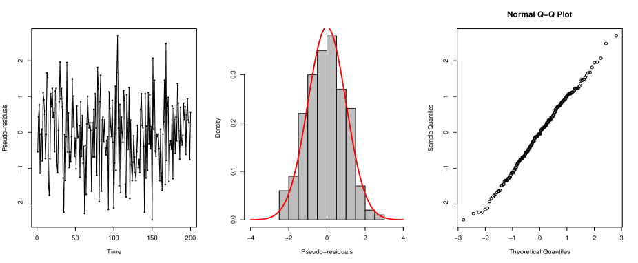
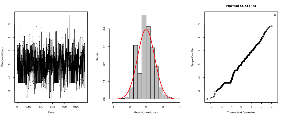
In order to assess the general goodness of fit of the models that we used in our experiments, we also investigated graphs of normal pseudo-residuals. Following Zucchini et al. (2017), the normal pseudo-residuals are defined as $$r_{t}=\Psi^{-1}\big{[}\,p\,(Y_{t}<y_{t}\,|\,\bm{y}^{(-t)},\,\bm{\eta})\,\big{]},$$ (A.5) where $\Psi$ is the cumulative distribution function of the standard normal distribution and the vector $\bm{y}^{(-t)}=(y_{1},\dots,y_{t-1},y_{t+1},\dots,y_{T})$ denotes all observations excluding $y_{t}$. If the model is accurate, $r_{t}$ is a realization of a standard normal random variable. We provide below index plots of the normal pseudo-residuals, their histograms and quantile-quantile (Q-Q) plots, for our main experiments. Figure A.1: Illustrative Example. Pseudo residuals: time series, histogram and Q-Q plot. Figure A.2: Telemetric Activity Data. Pseudo residuals: time series, histogram and Q-Q plot.

A.4 Telemetric Activity Data: Further Results

A.4.1 Estimated Dwell Distribution

Table 3 of the main paper provides point estimates for the parameters of the geometric (, Poisson and negative binomial dwell distributions of each of the nd tates. Figure A.3 here further plots the estimated posterior predictive distributions for the dwell length in each state. The estimated Poisson dwell distributions differ greatly from the geometric and negative binomial alternatives, in particular characterizing a much smaller variance in dwell times. The geometric and negative binomial provide more similar estimates of the dwell distribution, but notably for the nd tates the negative binomial assigns a larger probability to very short dwell times.

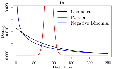
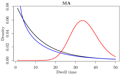
Figure A.3: Posterior predictive distribution for dwell time in nd tates under the geometric dwell) and Poisson and negative binomial

A.4.2 State Classification

We have further investigated the different state classifications provided by the optimal proposed model (using negative binomial durations) compared with the Poisson and geometric dwell distributions. Given the posterior means of the parameters of each dwell distribution, we estimated the most likely state sequence (using the Viterbi algorithm) and compared them using the confusion matrices presented in Table 1 below. From a state classification perspective, the negative binomial and geometric dwell durations perform similarly, while when choosing a Poisson durations we instead obtain significantly different results. This demonstrates the importance of estimating the dwell distribution in a data-driven manner, as different specifications of the dwell distribution can lead to vastly different inferential conclusions for objects of scientific interest. The values of the marginal likelihood, reported in Table 3 of the manuscript, suggest that there is evidence in favour of the ith negative binomial durations in comparison to a standard and to a substantially greater extent with respect to a Poisson dwell for this applied scenario.

Neg-Binom 458 5 0 40 382 66 0 1 198

Neg-Binom 498 0 0 0 385 0 0 3 264

Table A.1: State predictions summarized by the confusion matrix resulting from choosing different durations: (left) Poisson and negative binomial; (right) geometric and negative binomial.

A.5 Identifying the Periodicity

We describe the details of our Metropolis-within-Gibbs sampler to obtain posterior samples of the frequency $\omega$, the linear basis coefficients $\bm{\beta}$, and the residual variance $\sigma^{2}$, under the periodic model Eq. (6.2) of the main article. This sampling scheme follows closely the within-model move of the “segment model” introduced in Hadj-Amar et al. (2019, 2021), with the difference that in this case the number of frequencies is fixed to one. For our prior specification, we choose a uniform prior for the frequency $\omega\sim\text{Uniform}(0,0.1)$ and isotropic Gaussian prior for the vector of linear coefficients $\bm{\beta}=(\beta^{(1)},\beta^{(2)})$ $\sim\mathcal{\bm{N}}_{2}(\,\bm{0},\,\sigma^{2}_{\beta}\,\bm{I}\,)$, where the prior variance $\sigma^{2}_{\beta}$ is fixed at 5. The prior on the residual variance $\sigma^{2}$ is specified as $\text{Inverse-Gamma}\,\big{(}\frac{\xi_{0}}{2},\frac{\tau_{0}}{2}\big{)}$, where $\xi_{0}=4$ and $\tau_{0}=1$. For sampling the frequency, the proposal distribution is a combination of a Normal random walk centered around the current frequency and a sample from the periodogram, namely $$q\,(\,\omega^{\,p}\,|\,\omega^{\,c}\,)=\pi_{\omega}\,q_{1}\,(\,\omega^{\,p}\,|\,\omega^{\,c}\,)+(1-\pi_{\omega})\,q_{2}\,(\,\omega^{\,p}\,|\,\omega^{\,c}\,)$$ (A.6) where $q_{1}$ is defined in Eq. (A.7) below, $q_{2}$ is the density of a Normal $\mathcal{N}\,(\omega^{\,c},\sigma^{2}_{\omega})$, $\pi_{\omega}$ is a positive value such that $0\leq\pi_{\omega}\leq 1$, and the superscripts $c$ and $p$ refer to current and proposed values, respectively. For our experiments, we set $\sigma^{2}_{{\omega}}=1/(25T)$ and $\pi_{\omega}=0.1$. Eq. (A.6) states that a M-H step with proposal distribution $q_{1}\,(\,\omega^{\,p}\,|\,\omega^{\,c}\,)$ $$q_{1}\,(\,\omega^{\,p}\,|\,\omega^{\,c}\,)\propto\sum_{h\,=\,0}^{T-1}I_{h}\,\mathbbm{1}_{\big{[}\,h/T\,\,\leq\,\,\omega^{\,p}\,<\,\,(h+1)/T\,\big{]}\,},$$ (A.7) is performed with probability $\pi_{\omega}$, where $I_{h}$ is the value of the periodogram, namely the squared modulus of the Discrete Fourier transform evaluated at frequency $h/T$ I_h = 1T —   ∑_t=1^T y_t   exp(-i   2 π  hT   )  —^  2,  h = 0, …, T-1. The acceptance probability for this move is $$\alpha=\min\Bigg{\{}1,\dfrac{p\,(\omega^{\,p}\,|\,\bm{\beta},\,\sigma^{2},\,\bm{y})}{p\,(\omega^{\,c}\,|\,\bm{\beta},\,\sigma^{2},\,\bm{y})}\times\dfrac{q_{1}\,(\,\omega^{\,c}\,)}{q_{1}\,(\,\omega^{\,p}\,)}\Bigg{\}}.$$ On the other hand, with probability 1 - $\pi_{\omega}$, we perform random walk M-H step with proposal distribution $q_{2}\,(\,\omega^{\,p}\,|\,\omega^{\,c}\,)$, whose density is Normal with mean $\omega^{\,c}$ and variance $\sigma^{2}_{{\omega}}$, i.e. $\omega^{\,p}\,|\,\omega^{\,c}\,\sim\mathcal{N}(\,\omega^{\,c},\,\sigma^{2}_{{\omega}}\,)$. This move is accepted with probability $$\alpha=\min\Bigg{\{}1,\dfrac{p\,(\omega^{\,p}\,|\,\bm{\beta},\,\sigma^{2},\,\bm{y})}{p\,(\omega^{\,c}\,|\,\bm{\beta},\,\sigma^{2},\,\bm{y})}\Bigg{\}}.$$ Next, we update the vector of linear coefficients $\bm{\beta}$ and the residual variance $\sigma^{\,2}$ following the usual normal Bayesian regression setting (Gelman et al. 2013). Hence, $\bm{\beta}$ is updated in a Gibbs step from $$\bm{\beta}\,\big{|}\,\omega,\,\sigma^{2},\,\bm{y}\sim\bm{\mathcal{N}}_{2}\,(\,\hat{\bm{\beta}},\,\bm{V}_{\beta}),$$ (A.8) where $$\begin{split}\bm{V}_{\beta}&=\bigg{(}\sigma^{-2}_{\beta}\,\bm{I}+\sigma^{-2}\bm{X}(\omega)^{\,{}^{\prime}}\bm{X}(\omega)\bigg{)}^{-1},\\ \hat{\bm{\beta}}&=\bm{V}_{\beta}\,\big{(}\sigma^{-2}\bm{X}(\omega)^{\,{}^{\prime}}\bm{y}\big{)},\end{split}$$ (A.9) and we denote with $\bm{X}(\omega)$ the matrix with rows given by $\bm{x}_{t}\,\big{(}\omega\big{)}=[\cos(2\pi\omega t),\,\sin(2\pi\omega t)]$ for $t=1,\dots,T$. Finally, $\sigma^{\,2}$ is drawn in a Gibbs step directly from $$\sigma^{2}\,\big{|}\,\bm{\beta},\,\omega,\,\bm{y}\sim\text{Inverse-Gamma}\,\Bigg{(}\,\dfrac{T+\xi_{0}}{2},\,\dfrac{\tau_{0}+\sum_{t=1}^{T}\Big{\{}\,y_{t}-\bm{x}_{t}\,\big{(}\,\omega\,\big{)}^{\,{}^{\prime}}\,\bm{\beta}\,\Big{\}}^{2}}{2}\Bigg{)}.$$ (A.10)

References

https://mc-stan.org/docs/2_23/functions-reference/index.html