Operational Characterization of Multipartite Nonlocal Correlations

Abstract

Nonlocality, one of the most puzzling features of multipartite quantum correlation, has been identified as a useful resource for device-independent quantum information processing. Motivated by the resource theory of quantum entanglement recently an operational framework have been proposed by Gallego et al. [Phys. Rev. Lett. 109, 070401 (2012)] and Bancal et al. [Phys. Rev. A 88, 014102 (2013)] that characterizes the nonlocal resource present in multipartite quantum correlations. While the bipartite no-signaling correlations allows a dichotomous classification – local vs. nonlocal, in multipartite scenario the authors have shown existence of several types of nonlocality that are inequivalent under the proposed operational framework. In this work we present a finer characterization of multipartite no-signaling correlations based on the same operational framework. We also clarify a statement in Gallego et al.’s work that could be misinterpreted and make the conclusions of that work more precise here.

I Introduction

Nonlocality captures one of the important characteristic aspects of multipartite quantum systems. John S. Bell, in his seminal work Bell (1964), proved that a composite quantum system, prepared in suitable entangled state, can exhibit input-output correlations that can not be explained within the local realistic world view of classical physics Bell (1964, 1966) (see also Brunner et al. (2014); Mermin (1993)). Bell considered quantum system with two spatially separated subsystems and termed the joint input-output correlation locally-causal if it is product of input-output probabilities for the individual parties or convex mixture of individual input-output probabilities. He derived an empirically testable inequality whose violation establishes nonlocal nature of the correlation. Later, Svetlichny initiated the study of nonlocal correlations for multipartite quantum systems that involved more than two subsystems Svetlichny (1987). Following an apparently natural mathematical generalization of Bell he characterized multipartite correlations into three types - fully local, bilocal, and genuine nonlocal. He also came up with an empirical test to certify genuine nonlocality of a correlation. More recently, however, several groups of researchers identified that Svetlichny’s definition is stronger than needed, and suggested that the definition be modified to optimally capture the notion of genuineness in perfect operational sense Gallego et al. (2012); Bancal et al. (2013). They have also proposed a novel operational framework to address this issue.

The framework by Gallego et al. Gallego et al. (2012) is well motivated from resource theoretic perspective where the set of relevant free operations is identified as wirings and classical communication prior to the inputs (WCCPI). This framework introduces a hierarchical classification of multipartite correlations: set of no-signalling bilocal (NSBL) correlations $\subsetneq$ set of time-ordered bilocal correlations (TOBL) $\subsetneq$ set of general bilocal (BL) correlations $\subsetneq$ set of multipartite no-signalling (NS) correlations. The set BL is identical to the set of bilocal correlations as identified by Svetlichny and the correlations lying outside this set are called genuinely nonlocal. However, as pointed out in Gallego et al. (2012), a correlation even within the set BL may exhibit unexpected behaviour under WCCPI protocol. This consequently indicates genuine nonlocal nature of those BL correlations and therefore indicates that the framework of Svetlichny be improved to give a finer characterisation. In this work we revisit the framework of Gallego et al. While exploring their work we find that their framework is operationally perfect, but also that we should clarify some of their claims regarding the correlations presented there. Interestingly, we find that a more critical analysis of Ref. Gallego et al. (2012), in fact, introduces new classes of correlations lying in between the sets TOBL and BL. Our work thus can be viewed as culmination of the novel operational framework by Gallego et al. for characterizing the nonlocal correlations in multipartite scenario. The article is organized as follows: in section (II) we recall the operational frameworks for multipartite nonlocal correlations that have already been developed in the literature, in section (III) we present the main contribution of our work, and finally we put our conclusions in section (IV).

II Framework

Consider $n$ spatially separated parties. The input for $k^{th}$ party is denoted by $i_{k}$ and the corresponding outcome by $o_{k}$, with values taken from some finite set $\mathcal{I}_{k}$ and $\mathcal{O}_{k}$ respectively; $k\in\{1,\cdots,n\}$. An $n$-partite correlation is a joint input-output probability distribution $P:=\{p(o_{1}\cdots o_{n}|i_{1}\cdots i_{n})\leavevmode\nobreak\ |\leavevmode\nobreak\ p(o_{1}\cdots o_{n}|i_{1}\cdots i_{n})\geq 0\leavevmode\nobreak\ \forall\leavevmode\nobreak\ i_{k}\in\mathcal{I}_{k}\leavevmode\nobreak\ \&\leavevmode\nobreak\ o_{k}\in\mathcal{O}_{k};\leavevmode\nobreak\ \sum_{k}\sum_{o_{k}}p(o_{1}\cdots o_{n}|i_{1}\cdots i_{n})=1\leavevmode\nobreak\ \forall\leavevmode\nobreak\ i_{k}\in\mathcal{I}_{k}\}$. Such a correlation is called no-signaling if any non-empty subgroup of the parties can not change the marginal outcome probabilities for the remaining parties by changing their choice of inputs. Set of all NS correlations we will denote as $\mathcal{P}^{NS}_{n}$ or simply as $\mathcal{P}^{NS}$ when number of parties are not relevant to mention. Study of quantum nonlocality identifies physically motivated different hierarchical subsets of correlations in $\mathcal{P}^{NS}$. For instance, in two-party scenario a correlation is called local (Bell used the term locally-causal) if it can be expressed as,

$$p(o_{1}o_{2}|i_{1}i_{2})=\int_{\Lambda}p(\lambda)p(o_{1}|i_{1},\lambda)p(o_{2}|i_{2},\lambda)d\lambda,$$ (1)

where, $\lambda\in\Lambda$ is a random variable, commonly called local hidden variable in quantum foundation community, shared between the two parties following a probability distribution $\{p(\lambda)\leavevmode\nobreak\ |\leavevmode\nobreak\ p(\lambda)\geq 0\leavevmode\nobreak\ \&\leavevmode\nobreak\ \int p(\lambda)d\lambda=1\}$ over $\Lambda$. When $\lambda$ takes value from a discrete set, the above integral is replaced by summation. Bell came up with an empirical criterion, famously called the Bell inequality, to test whether a given correlation is local or not. Violation of this inequality establishes nonlocal nature of the correlation, i.e. the correlation can not be expressed as of Eq.(1). A correlation is called quantum if it can be obtained through quantum means, i.e. $P^{Q}:=\{p(o_{1}o_{2}|i_{1}i_{2})\equiv\mbox{Tr}[\rho_{12}(\pi^{i_{1}}_{o_{1}}\otimes\pi^{i_{2}}_{o_{2}})]\}$, where $\rho_{12}$ is a density operator acting on some composite Hilbert space $\mathcal{H}_{1}\otimes\mathcal{H}_{2}$ and $\{\pi^{i_{k}}_{o_{k}}\}$ be a positive operator valued measure (POVM) acting on $k^{th}$ parties Hilbert space, i.e. $\{\pi^{i_{k}}_{o_{k}}\geq 0,\leavevmode\nobreak\ \forall\leavevmode\nobreak\ i_{k}\in\mathcal{I}_{k},\leavevmode\nobreak\ o_{k}\in\mathcal{O}_{k},\leavevmode\nobreak\ \&\leavevmode\nobreak\ \sum_{o_{k}\in\mathcal{O}_{k}}\pi^{i_{k}}_{o_{k}}=\mathbf{I}_{k}\leavevmode\nobreak\ \forall\leavevmode\nobreak\ i_{k}\}$, with $\mathbf{I}_{k}$ being the identity operator on $\mathcal{H}_{k}$. Let us denote the set of local correlation and quantum correlation as $\mathcal{P}^{L}$ and $\mathcal{P}^{Q}$ respectively. While $\mathcal{P}^{NS}$ and $\mathcal{P}^{L}$ are convex polytope embedded in some Euclidean space, $\mathcal{P}^{Q}$ is a non-polytopic convex set with infinite, indeed unaccountably many infinite, number of extreme points. We have the following set inclusion relations

$$\mathcal{P}^{L}_{2}\subsetneq\mathcal{P}^{Q}_{2}\subsetneq\mathcal{P}^{NS}_{2}.$$ (2)

Whereas the proper set inclusion relation $\mathcal{P}^{L}_{2}\subsetneq\mathcal{P}^{Q}_{2}$ is established through Bell inequality violation, the inclusion relation $\mathcal{P}^{Q}_{2}\subsetneq\mathcal{P}^{NS}_{2}$ is assured from the example of correlation provided by Popescu & Rohrlich Popescu and Rohrlich (1994). Whenever cardinality of all the sets $\mathcal{I}_{1},\mathcal{I}_{2},\mathcal{O}_{1}$, and $\mathcal{O}_{2}$ is $2$, Fine Fine (1982) proved that a correlation $P$ will be in $\mathcal{P}^{L}_{2}$ if and only if it satisfies the Clauser-Horne-Shimony-Holt (CHSH) inequality Clauser et al. (1969). On the other hand the membership problem to decide whether a given correlation is quantum or not is in general undecidable Slofstra (2019a, b); Ji et al. (2020).

While in bipartite scenario the set of no-signaling correlations are characterized within local and nonlocal dichotomy, a finer characterization is required when the party number increases Svetlichny (1987). An $n$-partite input-output correlation is said to be fully local (FL) when

$$p(o_{1}\cdots o_{N}|i_{1}\cdots i_{N})=\int_{\Lambda}p(\lambda)\Pi_{k}p(o_{k}|i_{k},\lambda)d\lambda.$$ (3)

Outside the set $\mathcal{P}^{FL}$ there may exist correlations where nonlocality persists among $m(<n)$ parties but the remaining $n-m$ are locally correlated leading to different new classes of correlations. For instance, in tripartite scenario a correlation is called bilocal (BL) if it can be expressed as

$$p(o_{1}o_{2}o_{3}|i_{1}i_{2}i_{3})=\int p(\lambda)p(o_{1}|i_{1},\lambda)p(o_{2}o_{3}|i_{2}i_{3},\lambda)d\lambda.\leavevmode\nobreak\ \leavevmode\nobreak\ \leavevmode\nobreak\ \leavevmode\nobreak\$$ (4)

Correlations lying outside the set $\mathcal{P}^{BL}$ are called genuinely nonlocal. Note that, Svetlichny in his paper consider all party permutation while defining a BL correlation. However, here, likewise the Ref.Gallego et al. (2012), we will restrict ourselves in a particular party permutation, which will make no hindrance in the main purpose of this paper. In multipartite scenario, therefore, the set inclusion relations (2) get modified as,

$$\mathcal{P}^{FL}\subsetneq\mathcal{P}^{BL},\mathcal{P}^{Q}\subsetneq\mathcal{P}^{NS}.$$ (5)

Note that $\mathcal{P}^{BL}$ and $\mathcal{P}^{Q}$ do not follow any subset inclusion relation rather they overlap with each other, i.e. $\mathcal{P}^{BL}\cap\mathcal{P}^{Q}\neq\mathcal{P}^{BL},\mathcal{P}^{Q},\emptyset$.

Apart from foundational interest, the characterization of nonlocal correlations is also important from practical prospective as they have shown to be useful resource for device independent quantum information processing Scarani (2012). With this aim several groups have explored the notion of multipartite nonlocality in the recent past Gallego et al. (2012); Bancal et al. (2013). The framework in Gallego et al. (2012) is motivated from the resource theory of quantum entanglement, where entanglement is considered as a useful resource under the operational paradigm of local operation and classical communication (LOCC) Horodecki et al. (2009). In nonlocality scenario, the authors identified the free operations as WCCPI protocols under which the type of nonlocality should not be changed. However, they have pointed out that the a correlation that is local in $1$ vs $23$ ($1|23$) cut can exhibit nonlocality in the same cut after a bona fide WCCPI operation. Such an inconsistency challenges the completeness of the framework proposed by Svetlichny. The inconsistency stems from the fact that a term like $p(o_{2}o_{3}|i_{2}i_{3},\lambda)$ in the decomposition (4) does not need to satisfy the no-signaling constraint. Depending on whether such terms are no-signaling, one-way signaling, or two-way signaling, different sets of correlations can be defined.

Definition 1.

(PRL 109, 070401) A tripartite correlation $p(o_{1}o_{2}o_{3}|i_{1}i_{2}i_{3})\equiv P$ is said to admit a time-ordered bilocal (TOBL) model (with respect to the partition $1|23$) if it can be decomposed as,

$$P=\int p(\lambda)d\lambda p(o_{1}|i_{1},\lambda)p_{2\rightarrow 3}(o_{2}o_{3}|i_{2}i_{3},\lambda)$$ (6a)

$$=\int p(\lambda)d\lambda p(o_{1}|i_{1},\lambda)p_{2\leftarrow 3}(o_{2}o_{3}|i_{2}i_{3},\lambda),$$ (6b)

with the distributions $p_{2\rightarrow 3}$ and $p_{2\leftarrow 3}$ obeying the conditions

$$p_{2\rightarrow 3}(o_{2}|i_{2},\lambda)=\sum_{o_{3}}p_{2\rightarrow 3}(o_{2}o_{3}|i_{2}i_{3},\lambda),$$ (7a)

$$p_{2\leftarrow 3}(o_{3}|i_{3},\lambda)=\sum_{o_{2}}p_{2\leftarrow 3}(o_{2}o_{3}|i_{2}i_{3},\lambda).$$ (7b)

The above conditions tell that the term $p(o_{2}o_{3}|i_{2}i_{3},\lambda)$ allows only one-way signaling either $2^{nd}$ party to the $3^{rd}$ or vice verse. A tripartite correlation is called NSBL (BL) if the terms $p(o_{2}o_{3}|i_{2}i_{3},\lambda)$ obey the NS conditions in both ways (allows two way signalling). The authors in Gallego et al. (2012) have shown that TOBL correlations are consistent with WCCPI protocol along the partition $1|23$, i.e. such an operation maps TOBL correlations (6) into a probability distributions with a local model along this partition. They have also reported the following set inclusion relations in the correlation space,

$$\mathcal{P}^{FL}\subsetneq\mathcal{P}^{NSBL}\subsetneq\mathcal{P}^{TOBL}\subsetneq\mathcal{P}^{BL}\subsetneq\mathcal{P}^{NS}.$$ (8)

The proper set inclusion relation $\mathcal{P}^{TOBL}\subsetneq\mathcal{P}^{BL}$ has been established by providing an explicit example of quantum correlation in $\mathcal{P}^{BL}$ that exhibits unwanted nonlocal behavior along a particular partition ($1|23$ partition) even under bona fide WCCPI operation. Furthermore it has been claimed that the inconsistency is arising due to the presence of two-way signaling terms in its bi-local decomposition. In fact the authors in Gallego et al. (2012) have made an observation “Indeed, all the examples of distributions of the form (4) [also Eq.(4) in our paper] leading to a Bell violation under WCCPI have to be such that the bilocal decomposition requires terms displaying signalling in both directions". In the following section we will show that this particular sentence needs further clarification as it could be misleading, although the set inclusion relation (8) is flawless. However, we will show that a finer classification is possible than the subset inclusion relations of Eq.(8).

III Results

In this section, we first recall the example of correlation provided by Gallego et al. They have considered a tripartite quantum correlation obtained from the three-qubit GHZ state: $\ket{\psi_{GHZ}}_{123}=1/\sqrt{2}\left(\ket{000}+\ket{111}\right)_{A_{1}A_{2}A_{3}}$ shared among three parties (say) $A_{1},A_{2}$ and $A_{3}$. In each run, $A_{1}$ and $A_{2}$ perform one of two dichotomous measurements $\mathcal{M}:=\{\sigma_{z},\sigma_{x}\}$, whereas $A_{3}$ chooses her measurement from $\mathcal{M}^{\prime}:=\{(\sigma_{z}+\sigma_{x})/\sqrt{2},(\sigma_{z}-\sigma_{x})/\sqrt{2}\}$. Denoting the first measurement as input $0$ & the second one as $1$ and $+1$ outcome as $0$ & $-1$ as $1$ the resulting correlation can be expressed as the following matrix form:

$$P^{G}=\frac{1}{2}\left(\begin{array}[]{cccccccc}{2a^{+}}&{2a^{-}}&{0}&{0}&{0}&{0}&{2a^{-}}&{2a^{+}}\\ {2a^{+}}&{2a^{-}}&{0}&{0}&{0}&{0}&{2a^{-}}&{2a^{+}}\\ {a^{+}}&{a^{-}}&{a^{+}}&{a^{-}}&{a^{-}}&{a^{+}}&{a^{-}}&{a^{+}}\\ {a^{+}}&{a^{-}}&{a^{+}}&{a^{-}}&{a^{-}}&{a^{+}}&{a^{-}}&{a^{+}}\\ {a^{+}}&{a^{-}}&{a^{-}}&{a^{+}}&{a^{+}}&{a^{-}}&{a^{-}}&{a^{+}}\\ {a^{+}}&{a^{-}}&{a^{-}}&{a^{+}}&{a^{+}}&{a^{-}}&{a^{-}}&{a^{+}}\\ {a^{+}}&{a^{-}}&{a^{-}}&{a^{+}}&{a^{-}}&{a^{+}}&{a^{+}}&{a^{-}}\\ {a^{-}}&{a^{+}}&{a^{+}}&{a^{-}}&{a^{+}}&{a^{-}}&{a^{-}}&{a^{+}}\end{array}\right),$$ (9)

where $a^{\pm}:=1/4\left(1\pm 1/\sqrt{2}\right)$. We arrange the input in rows and output in columns and dictionary ordering is followed. This particular correlation is BL as it allows a decomposition (4) across $1|23$ partition and consequently $P^{G}$ should contain no nonlocal feature in that bi-partition. However, it turns out that after a bona fide WCCPI operation along $1|23$ cut, the resulting correlation $P=\{p(o_{1}o_{3}|i_{1}i_{2})\equiv\sum_{o_{2}}p(o_{1}o_{2}o_{3}|i_{1}i_{2},i_{3}=o_{2})\}$ exhibits CHSH inequality violation. In the required WCCPI protocol, $A_{2}$ and $A_{3}$ collaborate in the same laboratory while $A_{1}$ is in a spatially separated site. After the announcement of the inputs of the nonlocality task, $A_{2}$ produces her output $o_{2}$ using the input $i_{2}$ and then sends it to $A_{3}$ to use it as input $i_{3}$, i.e., $i_{3}=o_{2}$. Finally, $A_{3}$ yields output $o_{3}$. On the other side, $A_{1}$ locally produces output $o_{1}$ using input $i_{1}$. This clearly establishes the incompleteness of Svetlichny’s definitions of bilocality/ genuineness in relation to the operational paradigm of WCCPI. In the next, we show that the correlation $P^{G}$ allows a bilocal decomposition that contains terms with one-way signaling only.

Proposition 1.

The correlation $P^{G}$ allows a decomposition $P^{G}=\sum_{\lambda}p_{\lambda}p(o_{1}|i_{1},\lambda)p_{2\leftarrow 3}(o_{2}o_{3}|i_{2}i_{3},\lambda)$, where $p_{2\leftarrow 3}(o_{2}o_{3}|i_{2}i_{3},\lambda)$ does not admit signaling from $2$ to $3$ but (may) allow signaling from $3$ to $2$.

Proof.

The proof directly follows from the explicit decomposition given by,

$$P^{G}=\frac{1}{2}\begin{pmatrix}{1}&{0}\\ {1}&{0}\end{pmatrix}_{1}\otimes\begin{pmatrix}{a^{+}}&{a^{-}}&{0}&{0}\\ {a^{+}}&{a^{-}}&{0}&{0}\\ {a^{+}}&{a^{-}}&{0}&{0}\\ {0}&{0}&{a^{+}}&{a^{-}}\end{pmatrix}_{2\leftarrow 3}+\frac{1}{2}\begin{pmatrix}{1}&{0}\\ {0}&{1}\end{pmatrix}_{1}\otimes\begin{pmatrix}{a^{+}}&{a^{-}}&{0}&{0}\\ {a^{+}}&{a^{-}}&{0}&{0}\\ {0}&{0}&{a^{+}}&{a^{-}}\\ {a^{+}}&{a^{-}}&{0}&{0}\end{pmatrix}_{2\leftarrow 3}+\frac{1}{2}\begin{pmatrix}{0}&{1}\\ {1}&{0}\end{pmatrix}_{1}\otimes\begin{pmatrix}{0}&{0}&{a^{-}}&{a^{+}}\\ {0}&{0}&{a^{-}}&{a^{+}}\\ {0}&{0}&{a^{-}}&{a^{+}}\\ {a^{-}}&{a^{+}}&{0}&{0}\end{pmatrix}_{2\leftarrow 3}+\frac{1}{2}\begin{pmatrix}{0}&{1}\\ {0}&{1}\end{pmatrix}_{1}\otimes\begin{pmatrix}{0}&{0}&{a^{-}}&{a^{+}}\\ {0}&{0}&{a^{-}}&{a^{+}}\\ {a^{-}}&{a^{+}}&{0}&{0}\\ {0}&{0}&{a^{-}}&{a^{+}}\end{pmatrix}_{2\leftarrow 3}.$$ (10)

Please note that, the bipartite terms in the decomposition do not allow signaling from $2$ to $3$. ∎

This proves that a correlation does not require terms displaying signalling in both directions in its bilocal decomposition to show the inconsistent behaviour under WCCPI as claimed in Gallego et al. (2012). At this point, it is noteworthy that in the above decomposition we have terms that display signaling from $3$ to $2$ whereas the WCCPI protocol used to obtain a bipartite correlation in $1|23$ cut contains signaling from $2$ to $3$. This opposite directional signaling results in the ‘unwanted’ inconsistency. This observation motivates to define an asymmetric version of TOBL correlations.

Definition 2.

A tripartite correlation $p(o_{1}o_{2}o_{3}|i_{1}i_{2}i_{3})$ is said to admit a asymmetric time-ordered bilocal model from $3$ to $2$ if it allows a decomposition of the form $p(o_{1}o_{2}o_{3}|i_{1}i_{2}i_{3})=\sum p_{\lambda}p(o_{1}|i_{1},\lambda)p_{2\leftarrow 3}(o_{2}o_{3}|i_{2}i_{3},\lambda)$ but need not to allow a decomposition of the form $p(o_{1}o_{2}o_{3}|i_{1}i_{2}i_{3})=\sum p_{\lambda}p(o_{1}|i_{1},\lambda)p_{2\rightarrow 3}(o_{2}o_{3}|i_{2}i_{3},\lambda)$.

Collection of all such correlations we will denote as $\mathcal{P}^{ATOBL}_{2\leftarrow 3}$. Similarly, we can define the set $\mathcal{P}^{ATOBL}_{2\rightarrow 3}$. From Definition 1 & 2 arguably it follows that the set $\mathcal{P}^{TOBL}$ is intersection of these two asymmetric sets, $\mathcal{P}^{ATOBL}_{2\leftarrow 3}\cap\mathcal{P}^{ATOBL}_{2\rightarrow 3}=\mathcal{P}^{TOBL}$. Furthermore $\mathcal{P}^{TOBL}$ is a strict subset of both of them. To argue that, first note that the correlation (9) [from now on we will denote it as $P^{G}_{2\leftarrow 3}$] does not belong to the set $\mathcal{P}^{ATOBL}_{2\leftarrow 3}$, otherwise it will not show the nonlocality across $1|23$ partition under the WCCPI protocol displaying signaling from $3$ to $2$. Since $P^{G}_{2\leftarrow 3}\in\mathcal{P}^{ATOBL}_{2\leftarrow 3}$ but $P^{G}_{2\leftarrow 3}\notin\mathcal{P}^{ATOBL}_{2\rightarrow 3}$, therefor $P^{G}_{2\leftarrow 3}\notin\mathcal{P}^{TOBL}$ and hence $\mathcal{P}^{TOBL}\subsetneq\mathcal{P}^{ATOBL}_{2\leftarrow 3}$. One can obtain a correlation $P^{G}_{2\rightarrow 3}\in\mathcal{P}^{ATOBL}_{2\rightarrow 3}$ by just interchanging the measurements for $A_{2}$ and $A_{3}$ in $P^{G}_{2\leftarrow 3}$, i.e. $A_{2}$ chooses her measurement from the set $\mathcal{M}^{\prime}$ while $A_{3}$ from $\mathcal{M}$. To show the nonlocal behaviour of $P^{G}_{2\rightarrow 3}$ in the $1|23$ partition, one have to again interchange the role of $A_{2}$ and $A_{3}$ in the WCCPI that has been used for $P^{G}_{2\leftarrow 3}$. Applying similar argument as before it turns out that $\mathcal{P}^{TOBL}\subsetneq\mathcal{P}^{ATOBL}_{2\rightarrow 3}$.

We can define a set $\mathcal{P}^{ATOBL}$ of correlations which is the convex hull of $\mathcal{P}^{ATOBL}_{2\leftarrow 3}$ and $\mathcal{P}^{ATOBL}_{2\rightarrow 3}$, i.e.,

$$\mathcal{P}^{ATOBL} :=\{P\leavevmode\nobreak\ |\leavevmode\nobreak\ P=qP^{\prime}+(1-q)P^{\prime\prime}\},\leavevmode\nobreak\ \leavevmode\nobreak\ \leavevmode\nobreak\ \leavevmode\nobreak\ \leavevmode\nobreak\ \leavevmode\nobreak\$$ (11)

$$\mbox{with}\leavevmode\nobreak\ P^{\prime}, P^{\prime\prime}\in\mathcal{P}^{ATOBL}_{2\leftarrow 3}\leavevmode\nobreak\ \mbox{or}\leavevmode\nobreak\ \mathcal{P}^{ATOBL}_{2\rightarrow 3}\leavevmode\nobreak\ \&\leavevmode\nobreak\ q\in[0,1].$$

One can ask the question whether the set $\mathcal{P}^{ATOBL}$ is same as the set $\mathcal{P}^{ATOBL}_{2\leftarrow 3}\cup\mathcal{P}^{ATOBL}_{2\rightarrow 3}$. The following proposition answers this question in negative.

Proposition 2.

$\mathcal{P}^{ATOBL}_{2\leftarrow 3}\cup\mathcal{P}^{ATOBL}_{2\rightarrow 3}\subsetneq\mathcal{P}^{ATOBL}$.

Proof.

Consider the following two correlations

$$P^{\epsilon}_{2\leftarrow 3}=\frac{1}{2}\left(\begin{array}[]{cccccccc}{2k^{+}}&{2k^{-}}&{0}&{0}&{0}&{0}&{2k^{-}}&{2k^{+}}\\ {2k^{+}}&{2k^{-}}&{0}&{0}&{0}&{0}&{2k^{-}}&{2k^{+}}\\ {k^{+}}&{k^{-}}&{k^{+}}&{k^{-}}&{k^{-}}&{k^{+}}&{k^{-}}&{k^{+}}\\ {k^{+}}&{k^{-}}&{k^{+}}&{k^{-}}&{k^{-}}&{k^{+}}&{k^{-}}&{k^{+}}\\ {k^{+}}&{k^{-}}&{k^{-}}&{k^{+}}&{k^{+}}&{k^{-}}&{k^{-}}&{k^{+}}\\ {k^{+}}&{k^{-}}&{k^{-}}&{k^{+}}&{k^{+}}&{k^{-}}&{k^{-}}&{k^{+}}\\ {k^{+}}&{k^{-}}&{k^{-}}&{k^{+}}&{k^{-}}&{k^{+}}&{k^{+}}&{k^{-}}\\ {k^{-}}&{k^{+}}&{k^{+}}&{k^{-}}&{k^{+}}&{k^{-}}&{k^{-}}&{k^{+}}\end{array}\right),\leavevmode\nobreak\ \leavevmode\nobreak\ \leavevmode\nobreak\ \leavevmode\nobreak\ P^{\epsilon}_{2\rightarrow 3}=\frac{1}{2}\left(\begin{array}[]{cccccccc}{2k^{+}}&{0}&{2k^{-}}&{0}&{0}&{2k^{-}}&{0}&{2k^{+}}\\ {k^{+}}&{k^{+}}&{k^{-}}&{k^{-}}&{k^{-}}&{k^{-}}&{k^{+}}&{k^{+}}\\ {2k^{+}}&{0}&{2k^{-}}&{0}&{0}&{2k^{-}}&{0}&{2k^{+}}\\ {k^{+}}&{k^{+}}&{k^{-}}&{k^{-}}&{k^{-}}&{k^{-}}&{k^{+}}&{k^{+}}\\ {k^{+}}&{k^{-}}&{k^{-}}&{k^{+}}&{k^{+}}&{k^{-}}&{k^{-}}&{k^{+}}\\ {k^{+}}&{k^{-}}&{k^{-}}&{k^{+}}&{k^{-}}&{k^{+}}&{k^{+}}&{k^{-}}\\ {k^{+}}&{k^{-}}&{k^{-}}&{k^{+}}&{k^{+}}&{k^{-}}&{k^{-}}&{k^{+}}\\ {k^{-}}&{k^{+}}&{k^{+}}&{k^{-}}&{k^{+}}&{k^{-}}&{k^{-}}&{k^{+}}\end{array}\right),\leavevmode\nobreak\ \leavevmode\nobreak\ \leavevmode\nobreak\ \leavevmode\nobreak\$$ (12)

where, $k^{\pm}=1/4\left(1\pm\epsilon\right)$ with $0\leq\epsilon\leq 1$. Decomposition, analogous to Eq.(10), for these correlations are given by,

$$P^{\epsilon}_{2\leftarrow 3} =\frac{1}{2}\begin{pmatrix}{1}&{0}\\ {1}&{0}\end{pmatrix}\otimes\begin{pmatrix}{k^{+}}&{k^{-}}&{0}&{0}\\ {k^{+}}&{k^{-}}&{0}&{0}\\ {k^{+}}&{k^{-}}&{0}&{0}\\ {0}&{0}&{k^{+}}&{k^{-}}\end{pmatrix}+\frac{1}{2}\begin{pmatrix}{1}&{0}\\ {0}&{1}\end{pmatrix}\otimes\begin{pmatrix}{k^{+}}&{k^{-}}&{0}&{0}\\ {k^{+}}&{k^{-}}&{0}&{0}\\ {0}&{0}&{k^{+}}&{k^{-}}\\ {k^{+}}&{k^{-}}&{0}&{0}\end{pmatrix}+\frac{1}{2}\begin{pmatrix}{0}&{1}\\ {1}&{0}\end{pmatrix}\otimes\begin{pmatrix}{0}&{0}&{k^{-}}&{k^{+}}\\ {0}&{0}&{k^{-}}&{k^{+}}\\ {0}&{0}&{k^{-}}&{k^{+}}\\ {k^{-}}&{k^{+}}&{0}&{0}\end{pmatrix}+\frac{1}{2}\begin{pmatrix}{0}&{1}\\ {0}&{1}\end{pmatrix}\otimes\begin{pmatrix}{0}&{0}&{k^{-}}&{k^{+}}\\ {0}&{0}&{k^{-}}&{k^{+}}\\ {k^{-}}&{k^{+}}&{0}&{0}\\ {0}&{0}&{k^{-}}&{k^{+}}\end{pmatrix},$$ (13a)

$$P^{\epsilon}_{2\rightarrow 3} =\frac{1}{2}\begin{pmatrix}{1}&{0}\\ {1}&{0}\end{pmatrix}\otimes\begin{pmatrix}{k^{+}}&{0}&{k^{-}}&{0}\\ {k^{+}}&{0}&{k^{-}}&{0}\\ {k^{+}}&{0}&{k^{-}}&{0}\\ {0}&{k^{+}}&{0}&{k^{-}}\end{pmatrix}+\frac{1}{2}\begin{pmatrix}{1}&{0}\\ {0}&{1}\end{pmatrix}\otimes\begin{pmatrix}{k^{+}}&{0}&{k^{-}}&{0}\\ {0}&{k^{+}}&{0}&{k^{-}}\\ {k^{+}}&{0}&{k^{-}}&{0}\\ {k^{+}}&{0}&{k^{-}}&{0}\end{pmatrix}+\frac{1}{2}\begin{pmatrix}{0}&{1}\\ {1}&{0}\end{pmatrix}\otimes\begin{pmatrix}{0}&{k^{-}}&{0}&{k^{+}}\\ {0}&{k^{-}}&{0}&{k^{+}}\\ {0}&{k^{-}}&{0}&{k^{+}}\\ {k^{-}}&{0}&{k^{+}}&{0}\end{pmatrix}+\frac{1}{2}\begin{pmatrix}{0}&{1}\\ {0}&{1}\end{pmatrix}\otimes\begin{pmatrix}{0}&{k^{-}}&{0}&{k^{+}}\\ {k^{-}}&{0}&{k^{+}}&{0}\\ {0}&{k^{-}}&{0}&{k^{+}}\\ {0}&{k^{-}}&{0}&{k^{+}}\end{pmatrix}.$$ (13b)

Consider now another correlation $P^{\epsilon}_{\alpha}$ obtained by convex mixing of the correlations in Eq.(12),

$$P^{\epsilon}_{\alpha}=\alpha P^{\epsilon}_{2\leftarrow 3}+(1-\alpha)P^{\epsilon}_{2\rightarrow 3}\leavevmode\nobreak\ ;\leavevmode\nobreak\ \leavevmode\nobreak\ \leavevmode\nobreak\ \alpha\in[0,1].$$ (14)

As in the case of $P^{G}$ if we apply the same WCCPI operations containing signaling $2\twoheadleftarrow 3$ and $2\twoheadrightarrow 3$ not we will obtain the respective bipartite correlations across the $1|23$ partition:

$$Q_{2\twoheadleftarrow 3}(\epsilon,\alpha) :=\{p(o_{1}o_{3}|i_{1}i_{2})\}\equiv\frac{1}{2}\begin{pmatrix}{2k^{+}+\alpha k^{-}}&{(2-\alpha)k^{-}}&{\alpha k^{+}+2(1-\alpha)k^{-}}&{(2-\alpha)k^{+}+2\alpha k^{-}}\\ {2k^{+}+\alpha k^{-}}&{(2-\alpha)k^{-}}&{\alpha k^{+}+2(1-\alpha)k^{-}}&{(2-\alpha)k^{+}+2\alpha k^{-}}\\ {\frac{1}{2}}&{\frac{1}{2}}&{(\alpha+1)k^{+}+(1-\alpha)k^{-}}&{(1-\alpha)k^{+}+(\alpha+1)k^{-}}\\ {2k^{+}}&{2k^{-}}&{\alpha k^{+}+(2-\alpha)k^{-}}&{(2-\alpha)k^{+}+\alpha k^{-}}\end{pmatrix},$$ (15a)

$$Q_{2\twoheadrightarrow 3}(\epsilon,\alpha) :=\{p(o_{1}o_{2}|i_{1}i_{3})\}\equiv\frac{1}{2}\begin{pmatrix}{2k^{+}+(1-\alpha)k^{-}}&{(\alpha+1)k^{-}}&{(1-\alpha)k^{+}+2\alpha k^{-}}&{(\alpha+1)k^{+}+2(1-\alpha)k^{-}}\\ {2k^{+}+(1-\alpha)k^{-}}&{(\alpha+1)k^{-}}&{(1-\alpha)k^{+}+2\alpha k^{-}}&{(\alpha+1)k^{+}+2(1-\alpha)k^{-}}\\ {\frac{1}{2}}&{\frac{1}{2}}&{(2-\alpha)k^{+}+\alpha k^{-}}&{\alpha k^{+}+(2-\alpha)k^{-}}\\ {2k^{+}}&{2k^{-}}&{(1-\alpha)k^{+}+(\alpha+1)k^{-}}&{(\alpha+1)k^{+}+(1-\alpha)k^{-}}\end{pmatrix}.$$ (15b)

The Bell-CHSH values for these correlations turn out to be

$$\mathcal{B}_{2\twoheadleftarrow 3}(\epsilon,\alpha) =\alpha+\epsilon(3-2\alpha),\leavevmode\nobreak\ \leavevmode\nobreak\ \leavevmode\nobreak\ \leavevmode\nobreak\ \leavevmode\nobreak\ \leavevmode\nobreak\ \mathcal{B}_{2\twoheadrightarrow 3}(\epsilon,\alpha)=(1-\alpha)+\epsilon(1+2\alpha).$$ (16)

When $P^{\epsilon}_{2\leftarrow 3}$ and $P^{\epsilon}_{2\rightarrow 3}$ are mixed equally, the resulting bipartite correlations obtained under two different WCCPI protocols are same, i.e. $Q_{2\twoheadleftarrow 3}(\epsilon,1/2)=Q_{2\twoheadrightarrow 3}(\epsilon,1/2):=Q(\epsilon,1/2)$, and consequently their Bell-CHSH values, $\mathcal{B}_{2\twoheadleftarrow 3}(\epsilon,1/2)=\mathcal{B}_{2\twoheadrightarrow 3}(\epsilon,1/2):=\mathcal{B}(\epsilon,1/2)=1/2+2\epsilon$. This leads us to the following conclusion. If the correlation $P^{\epsilon}_{1/2}$ can be shown to be lie outside the set $\mathcal{P}^{ATOBL}_{2\rightarrow 3}$ then it must also lie outside $\mathcal{P}^{ATOBL}_{2\leftarrow 3}$. Since $Q(\epsilon,1/2)$ exhibits nonlocality for $\epsilon>3/4$, therefore the correlations $P^{\epsilon>3/4}_{\alpha=1/2}$ (:=$P^{>3/4}_{1/2}$) lie outside the set $\mathcal{P}^{ATOBL}_{2\rightarrow 3}\cup\mathcal{P}^{ATOBL}_{2\leftarrow 3}$. On the other hand, by construction we have $P^{>3/4}_{1/2}\in\mathcal{P}^{ATOBL}$, which thus implies Proposition 2. ∎

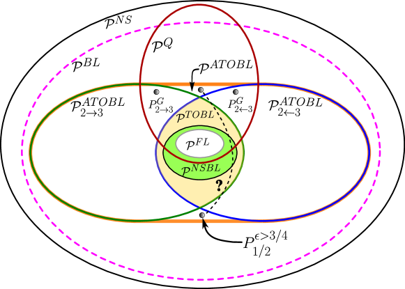
Figure 1: [Color on-line] The inner most white region represents the set of fully local correlations. This and green region represent the set of NSBL correlations. Intersection of the two asymmetric sets $\mathcal{P}^{ATOBL}_{2\leftarrow 3}$ and $\mathcal{P}^{ATOBL}_{2\rightarrow 3}$ (blue and green elliptical regions, respectively) is the the set of TOBL correlations and their convex hull $\mathcal{P}^{ATOBL}$ is strictly larger than their union. The set $\mathcal{P}^{BL}$ of BL correlations are shown by purple dotted region. It is shown by dotted line as we have not proved $\mathcal{P}^{ATOBL}\subsetneq\mathcal{P}^{BL}$, although we believe the proper inclusion should hold. Red elliptical region $\mathcal{P}^{Q}$ denotes the set of quantum correlations which strictly contains $\mathcal{P}^{FL}$ but only overlaps with all other sets. For instance the tripartite correlation $P_{1}\otimes P^{PR}_{23}$ is a non quantum NSBL correlation, where $P$ is some single party input-output probability vector and $P^{PR}$ is the Popescu-Rohrlich correlation. Outermost black ellipse denotes the set of all NS correlations. We put the ‘?’ mark as we are not sure whether the correlation $P^{>3/4}_{1/2}$ is quantum or not.

Thus compared to Eq.(8) we have the following finer set inclusion relations in the correlations space.

$$\mathcal{P}^{FL}\subsetneq\mathcal{P}^{NSBL}\subsetneq\mathcal{P}^{TOBL}\subsetneq\mathcal{P}^{ATOBL}_{2\rightarrow 3},\mathcal{P}^{ATOBL}_{2\leftarrow 3}$$

$$\subsetneq\mathcal{P}^{ATOBL}_{2\rightarrow 3}\cup\mathcal{P}^{ATOBL}_{2\leftarrow 3}\subsetneq\mathcal{P}^{ATOBL}\subseteq\mathcal{P}^{BL}\subsetneq\mathcal{P}^{NS}.$$ (17)

We have not been able to prove the proper subset relation $\mathcal{P}^{ATOBL}\subsetneq\mathcal{P}^{BL}$, although we believe it should hold. Also note that, we have only prove that the correlations $P^{>3/4}_{1/2}$ live in $\mathcal{P}^{ATOBL}$ but not in $\mathcal{P}^{ATOBL}_{2\leftarrow 3}\cup\mathcal{P}^{ATOBL}_{2\rightarrow 3}$. However, we don’t know whether these correlations are quantum or not. The essence of our study can be presented in a Venn diagram as depicted in Fig.1.

IV Discussions

Bell’s theorem addresses one of the long standing debate regarding the foundational status of quantum theory Einstein et al. (1935); Bohr (1935); Schrödinger (1935); Neu ; Bohm (1952a, b); Gleason (1957); Jauch and Piron (1963) and shakes one of our most inveterate world view. Advent of quantum information theory identifies Bell nonlocality as a useful resource for device independent quantum information processing where an information task can be achieved without making any assumptions about the internal working of the devices used in the protocol. Several such protocols have been proposed with many of them already achieving practical implementation Acín et al. (2006); Pironio et al. (2010); Colbeck and Renner (2012); Brunner et al. (2008); Das et al. (2013); Mukherjee et al. (2015); Chaturvedi and Banik (2015); et al. (2017). It has also been established as useful resource in Bayesian game theory to Brunner and Linden (2013); Roy et al. (2016); Banik et al. (2019). Resource quantification and characterization of such nonlocal correlations is, therefore, relevant from practical point of view. In this paper, we revisit one such framework for multipartite nonlocality developed in Ref.Gallego et al. (2012). We show that a finer characterization of multipartite nonlocal correlations than that of Ref.Gallego et al. (2012) is possible under the same operational framework proposed there. While doing so we also find some potentially confusing statements made in Gallego et al. (2012) and restate those. Our work accompanying with Ref.Gallego et al. (2012) thus provide a comprehensible picture of multipartite nonlocal correlations.

References

• Bell (1964) J. S. Bell, “On the Einstein Podolsky Rosen Paradox,” Physics 1, 195 (1964).
• Bell (1966) J. S. Bell, “On the Problem of Hidden Variables in Quantum Mechanics,” Rev. Mod. Phys. 38, 447 (1966).
• Brunner et al. (2014) N. Brunner, D. Cavalcanti, S. Pironio, V. Scarani,  and S. Wehner, “Bell nonlocality,” Rev. Mod. Phys. 86, 419–478 (2014).
• Mermin (1993) N. D. Mermin, “Hidden variables and the two theorems of john bell,” Rev. Mod. Phys. 65, 803–815 (1993).
• Svetlichny (1987) G. Svetlichny, “Distinguishing three-body from two-body nonseparability by a bell-type inequality,” Phys. Rev. D 35, 3066–3069 (1987).
• Gallego et al. (2012) R. Gallego, L. E. Würflinger, A. Acín,  and M. Navascués, “Operational framework for nonlocality,” Phys. Rev. Lett. 109, 070401 (2012).
• Bancal et al. (2013) J.-D. Bancal, J. Barrett, N. Gisin,  and S. Pironio, “Definitions of multipartite nonlocality,” Phys. Rev. A 88, 014102 (2013).
• Popescu and Rohrlich (1994) S. Popescu and D. Rohrlich, “Quantum nonlocality as an axiom,” Found. Phys. 24, 379–385 (1994).
• Fine (1982) A. Fine, “Hidden Variables, Joint Probability, and the Bell Inequalities,” Phys. Rev. Lett. 48, 291–295 (1982).
• Clauser et al. (1969) J. F. Clauser, M. A. Horne, A. Shimony,  and R. A. Holt, “Proposed Experiment to Test Local Hidden-Variable Theories,” Phys. Rev. Lett. 23, 880–884 (1969).
• Slofstra (2019a) W. Slofstra, “The set of quantum correlations is not closed,” Forum Math. Pi 7, e1 (2019a), (arXiv:1703.08618).
• Slofstra (2019b) W. Slofstra, “Tsirelson’s problem and an embedding theorem for groups arising from non-local games,” J. Am. Math. Soc 33, 1–56 (2019b), (arXiv:1606.03140).
• Ji et al. (2020) Z. Ji, A. Natarajan, T. Vidick, J. Wright,  and H. Yuen, “MIP*=RE,”  (2020), arXiv:2001.04383 [quant-ph] .
• Scarani (2012) V. Scarani, “The device-independent outlook on quantum physics,” Acta Phys. Slovaca 62, 347–409 (2012).
• Horodecki et al. (2009) R. Horodecki, P. Horodecki, M. Horodecki,  and K. Horodecki, “Quantum entanglement,” Rev. Mod. Phys. 81, 865–942 (2009).
• (16)  Here, double arrow ‘$2\twoheadleftarrow 3$’ denotes WCCPI operation with communication from $A_{3}$ to $A_{2}$ as described previously, while ‘$2\twoheadrightarrow 3$’ implies the opposite.
• Einstein et al. (1935) A. Einstein, B. Podolsky,  and N. Rosen, “Can Quantum-Mechanical Description of Physical Reality Be Considered Complete?” Phys. Rev. 47, 777–780 (1935).
• Bohr (1935) N. Bohr, “Can quantum-mechanical description of physical reality be considered complete?” Phys. Rev. 48, 696–702 (1935).
• Schrödinger (1935) E. Schrödinger, “Discussion of Probability Relations between Separated Systems,” Proc. Cambridge Philos. Soc. 31, 553 (1935).
• (20)  J. von Neumann, “Mathematishe Grundlagen der Quanten-mechanik", Verlag Julius-Springer, Berlin (1932), [English translation: Princeton University Press (1955)].
• Bohm (1952a) D. Bohm, “A Suggested Interpretation of the Quantum Theory in Terms of "Hidden" Variables. I,” Phys. Rev. 85, 166–179 (1952a).
• Bohm (1952b) D. Bohm, “A Suggested Interpretation of the Quantum Theory in Terms of "Hidden" Variables. II,” Phys. Rev. 85, 180–193 (1952b).
• Gleason (1957) A. M. Gleason, “Measures on the closed subspaces of a Hilbert space,” J. Math. Mech. 6, 885–893 (1957).
• Jauch and Piron (1963) J. M. Jauch and C. Piron, “Can hidden variables be excluded in quantum mechanics,” Helv. Phys. Acta 36, 827–837 (1963).
• Acín et al. (2006) A. Acín, N. Gisin,  and L. Masanes, “From Bell’s Theorem to Secure Quantum Key Distribution,” Phys. Rev. Lett. 97, 120405 (2006).
• Pironio et al. (2010) S. Pironio, A. Acín, S. Massar, A. Boyer de la Giroday, D. N. Matsukevich, P. Maunz, S. Olmschenk, D. Hayes, L. Luo, T. A. Manning,  and C. Monroe, “Random numbers certified by Bell’s theorem,” Nature 464, 1021–1024 (2010).
• Colbeck and Renner (2012) R. Colbeck and R. Renner, “Free randomness can be amplified,” Nat. Phys. 8, 450–453 (2012).
• Brunner et al. (2008) N. Brunner, S. Pironio, A. Acín, N. Gisin, A. A. Méthot,  and V. Scarani, “Testing the Dimension of Hilbert Spaces,” Phys. Rev. Lett. 100, 210503 (2008).
• Das et al. (2013) S. Das, M. Banik, A. Rai, Md. R. Gazi,  and S. Kunkri, “Hardy’s nonlocality argument as a witness for postquantum correlations,” Phys. Rev. A 87, 012112 (2013).
• Mukherjee et al. (2015) A. Mukherjee, A. Roy, S. S. Bhattacharya, S. Das, Md. R. Gazi,  and M. Banik, “Hardy’s test as a device-independent dimension witness,” Phys. Rev. A 92, 022302 (2015).
• Chaturvedi and Banik (2015) A. Chaturvedi and M. Banik, “Measurement-device–independent randomness from local entangled states,” EPL 112, 30003 (2015).
• et al. (2017) J. Yin et al., “Satellite-based entanglement distribution over 1200 kilometers,” Science 356, 1140–1144 (2017).
• Brunner and Linden (2013) N. Brunner and N. Linden, “Connection between Bell nonlocality and Bayesian game theory,” Nat. Comm. 4, 2057 (2013).
• Roy et al. (2016) A. Roy, A. Mukherjee, T. Guha, S. Ghosh, S. S. Bhattacharya,  and M. Banik, “Nonlocal correlations: Fair and unfair strategies in Bayesian games,” Phys. Rev. A 94, 032120 (2016).
• Banik et al. (2019) M. Banik, S. S. Bhattacharya, N. Ganguly, T. Guha, A. Mukherjee, A. Rai,  and A. Roy, “Two-qubit pure entanglement as optimal social welfare resource in bayesian game,” Quantum 3, 185 (2019).