Resolving the puzzle of sound propagation in liquid helium at low temperatures

Abstract

Experimental data suggests that, at temperatures below 1 K, the pressure in liquid helium has a cubic dependence on density. Thus the speed of sound scales as a cubic root of pressure. Near a critical pressure point, this speed approaches zero whereby the critical pressure is negative, thus indicating a cavitation instability regime. We demonstrate that to explain this dependence, one has to view liquid helium as a mixture of three quantum Bose liquids: dilute (Gross-Pitaevskii-type) Bose-Einstein condensate, Ginzburg-Sobyanin-type fluid, and logarithmic superfluid. Therefore, the dynamics of such a mixture is described by a quantum wave equation, which contains not only the polynomial (Gross-Pitaevskii and Ginzburg-Sobyanin) nonlinearities with respect to a condensate wavefunction, but also a non-polynomial logarithmic nonlinearity. We derive an equation of state and speed of sound in our model, and show their agreement with experiment.

I Introduction

The velocity of ordinary (“first”) sound in liquid helium at temperatures below 1 K was measured with great accuracy as a function of both temperature wc62 ; wc67 and pressure abraham1 ; abraham2 . An analysis of experimental data by Abraham et al. reveals that sound velocity $c_{s}$ decreases with pressure as a cubic root, cf. Fig. 1:

$$c_{s}=K^{1/3}(P-P_{c})^{\nu},\ \nu=\tfrac{1}{3}\pm 0.01,$$ (1)

where the critical pressure being about $P_{c}=-9.52$ and $-3.11$ atm for ${}^{4}\text{He}$ and ${}^{3}\text{He}$ respectively, whereas $K=1.41\times 10^{6}$ $\text{cm}^{4}\,\text{g}^{-1}\,\text{s}^{-1}$ and $1.93\times 10^{6}$ $\text{cm}^{4}\,\text{g}^{-1}\,\text{s}^{-1}$ for ${}^{4}\text{He}$ and ${}^{3}\text{He}$ respectively; negative values indicate that zero velocity of sound occurs in the cavitation regime where nucleation of bubbles causes a macroscopic instability. On the other hand, conventional arguments imply that in the vicinity of the critical pressure point $P_{c}$ the speed of sound should scale as a quartic root of pressure, $c\propto(P-P_{c})^{1/4}$, which disagrees with both experiment and numerical simulations mar91 ; mar94 ; mar95 ; Qu ; bauer ; dalfovo ; boronat ; edwards . These arguments rely heavily on approximations and perturbation techniques, which are usually pertinent to systems of weakly interacting bosons, such as dilute Bose-Einstein condensates, where two-body contact interactions are predominant and non-perturbative effects are neglected.

In this paper, we propose a non-perturbative approach, which takes into account multi-body interactions in liquid helium and explains the experimental data by Abraham et al., including an equation of state and the relation (1).

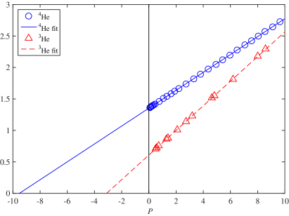
Figure 1: Profile of $c_{s}^{3}$ in units of $10^{13}\text{cm}^{3}/\text{s}^{3}$, versus pressure $P$, in atm. The experimental data was taken from Refs. abraham1 ; abraham2 , for ⁴He (circles, solid fitting curve) and ³He (triangles, dashed fitting curve).

II Model

After the discovery of Bose-Einstein condensation and related phenomena, it was established that quantum Bose liquids are not a discrete set of particles, such as helium atoms, interacting via some interparticle potential. Instead, a new phenomenon occurs: the discreteness of the atoms is averaged out, collective degrees of freedoms emerge, which are no longer identical to constituent particles, and the whole system becomes essentially nonlocal and continuous ant03 . Correspondingly, wavefunctions describing these new degrees of freedom are to be considered fundamental within the frameworks of the collective approach. Even for ground states, these condensate wavefunctions do not obey the conventional (linear) Schrödinger equations, but some nonlinear quantum wave equations in which nonlinearities account for many-body effects gs76 ; gs82 ; jpr95 . Our task here will be to determine a form of those equations, starting from some minimal model assumptions followed by fixing their parameters using experimental data.

In a theory of quantum Bose liquids and Bose-Einstein condensates, one introduces a complex-valued condensate wavefunction $\Psi=\Psi(\textbf{x},t)$, which obeys a normalization condition

$$\int_{V}|\Psi|^{2}dV=\int_{V}\rho dV={M}=m{N},$$ (2)

where ${M}$, $V$ and ${N}$ are, respectively, the total mass, volume, and particles’ number of the fluid, $\rho=|\Psi|^{2}$ is the fluid mass density, and $m=m_{\text{He}}$ is the mass of the constituent particle. This condition imposes restrictions upon the condensate wavefunctions, which reveals its quantum mechanical nature: the set of all normalizable functions $\Psi$ which constitutes a Hilbert space, such as $L^{2}$.

For physical configurations, the function $\Psi$ must minimize the action functional $\iint_{V}{\cal L}\,dVdt$, where the Lagrangian density has a Galilean-invariant $U(1)$-symmetric form:

$${\cal L}=\frac{i\hbar}{2}(\Psi\partial_{t}\Psi^{*}-\Psi^{*}\partial_{t}\Psi)+\frac{\hbar^{2}}{2m}|\boldsymbol{\nabla}\Psi|^{2}+V_{\text{ext}}\,|\Psi|^{2}+{\cal V}(|\Psi|^{2}),$$ (3)

where $V_{\text{ext}}=V_{\text{ext}}(\textbf{x},t)$ is an external or trapping potential, and ${\cal V}(|\Psi|^{2})$ is an effective many-body interaction potential density. We write the latter in the series form, to be explained as follows:

$${\cal V}(\rho) = {\cal V}_{(\text{ln})}(\rho)+\sum\limits_{k=2}^{\cal N}{\cal V}_{(k)}(\rho),$$ (4)

$${\cal V}_{(\text{ln})}(\rho) = \epsilon C_{(\text{ln})}\rho\left[1-\ln{\left(\rho/\bar{\rho}\right)}\right],$$

$${\cal V}_{(k)}(\rho) = \epsilon C_{(k)}\bar{\rho}\left(\rho/\bar{\rho}\right)^{k},$$

where $\epsilon$ and $\bar{\rho}$ are scale constants with the dimensions of energy and mass density, respectively, and the $C$’s are dimensionless coupling coefficients whose values are to be established below; the index $k$ labels the $k$th-order contact interaction potential with respect to $\rho$. The couplings $C$’s do not depend on the mass density $\rho$, but they can be functions of the thermodynamic parameters of the fluid.

By applying the Euler-Lagrange variational principle to eqs. (3), (4), we obtain the following quantum wave equation:

$$\left[-i\hbar\,\partial_{t}-\frac{\hbar^{2}}{2m}\vec{\nabla}^{2}+V_{\text{ext}}(\vec{x},\,t)+F(|\Psi|^{2})\right]\Psi=0,$$ (5)

where

$$F(\rho) = \frac{d}{d\rho}{\cal V}(\rho)=F_{(\text{ln})}(\rho)+\sum\limits_{k=2}^{\cal N}F_{(k)}(\rho),$$ (6)

$$F_{(\text{ln})}(\rho) = -\epsilon C_{(\text{ln})}\ln{\!\left(\rho/\bar{\rho}\right)},$$

$$F_{(k)}(\rho) = \epsilon kC_{(k)}\left(\rho/\bar{\rho}\right)^{k-1}.$$

Equations (4)-(6) indicate that the Bose liquid in our model has the following multi-component structure:

First, the potential term ${\cal V}_{(\text{ln})}\propto|\Psi|^{2}\left[1-\ln{\left(|\Psi|^{2}/\bar{\rho}\right)}\right]$ describes the logarithmic fluid component and induces the logarithmic nonlinearity $F_{(\text{ln})}\propto\ln{\left(|\Psi|^{2}/\bar{\rho}\right)}$ in the wave equation (5). Nonlinearity of this type often occurs in field theories of particles and gravity ros68 ; ros69 ; bb76 ; em98 ; z10gc ; z11appb ; dz11 ; scott1 ; dmz15 ; scott2 , as well as in the classical and quantum mechanics of various fluids z11appb ; dmf03 ; gl08 ; az11 ; z12eb ; bo15 ; z17zna ; z18epl ; z18zna . The reason for such universality is that logarithmically nonlinear terms readily emerge in evolution equations for those dynamical systems in which interparticle interaction energies dominate kinetic ones z18zna . Such systems include not only low-temperature gases and liquids az11 ; z12eb , but also hot dense matter and effectively lower-dimensional flows dmf03 ; z18epl .

In particular, a significant amount of experimental evidence supports universal applicability of logarithmic models in the theory of superfluidity of ⁴He. The logarithmic fluid turns out to be very instrumental for describing the microscopic properties of the superfluid component of ⁴He: it analytically reproduces with high accuracy the three main observable facts of this liquid – the Landau spectrum of excitations, the structure factor, and the speed of sound at normal pressure, while using only one non-scale parameter to fit the excitation spectrum’s experimental data z12eb .

It should be mentioned here that the logarithmic nonlinearity readily occurs if one attempts to renormalize perturbative models of liquid helium and take into account zero-point oscillations therein mar94 . From that prospective, the logarithmic term can be interpreted as a cumulative macroscopical effect of the quantum interaction between the collective degrees of freedom of superfluid helium and virtual particles, which correlates with an idea of using the logarithmic fluids for a non-perturbative description of the physical vacuum as such z11appb .

Second, the component described by the Ginzburg-Landau-type (quartic) potential ${\cal V}_{(2)}\propto|\Psi|^{4}$, represents a well-known Gross-Pitaevskii (GP) condensate where the interparticle interaction can be well approximated by a 2-body potential made of a contact (delta-singular) shape gr61 ; pi61 . This approximation is robust in dilute Bose-Einstein condensates, but for strongly-interacting quantum liquids, it cannot be used as a leading-order approximation. However, it can still make a viable contribution.

Third, the fluid described by the sextic term, ${\cal V}_{(3)}\propto|\Psi|^{6}$, is another beyond-GP-approximation term, as discussed by Ginzburg and Sobyanin gs76 ; gs82 . This term is related to three-particle interactions: for instance, it can be induced by the trimer bound states in liquid helium discovered by Efimov ef71 ; ef73 , a recent review of literature can be found in kms11 . Another source of six-order terms with respect to $|\Psi|$ could be fermionic admixtures cr04 ; crt04 and the reduction of a fluid’s effective dimensionality ks92 .

Finally, the higher-order polynomial potential terms ${\cal V}_{(k)}\propto|\Psi|^{2k}$, where $k>3$, can also occur in strongly-interacting Bose liquids. However, their substantial influence on the physics of liquid helium has, to the best of our knowledge, not been reported yet. Below it will be demonstrated that such terms can be neglected for the purposes of this paper.

Using the Madelung representation of a wavefunction, one can rewrite any nonlinear wave equation of the type (5) in hydrodynamic form. One can show that the corresponding fluid has an equation of state and speed of sound $c_{s}$, which are given by the following general formulae z11appb :

$$P(\rho) \approx P_{0}-\frac{\hbar}{m}\int\rho\,dF(\rho),$$ (7)

$$c_{s} = \sqrt{\frac{dP(\rho)}{d\rho}}\approx\sqrt{-\frac{\hbar\,\rho}{m}\frac{dF(\rho)}{d\rho}},$$ (8)

where $P_{0}$ is an arbitrary constant, and the approximation symbol means that we keep only the leading-order terms with respect to the Planck constant; a detailed derivation of these formulae can be found, e.g., in Sec. 3.1 of z19mat .

When evaluated on a function (6), formulae (7) and (8) yield an equation of state and speed of sound for our model:

$$P \approx P_{0}+\frac{\hbar\epsilon}{m}\left[C_{(\text{ln})}\rho-\bar{\rho}\sum\limits_{k=2}^{\cal N}(k-1)C_{(k)}\left(\rho/\bar{\rho}\right)^{k}\right]\!,~{}~{}~{}$$ (9)

$$c_{s}^{2} \approx \frac{\hbar\epsilon}{m}\left[C_{(\text{ln})}-\bar{\rho}\sum\limits_{k=2}^{\cal N}k(k-1)C_{(k)}\left(\rho/\bar{\rho}\right)^{k-1}\right]\!.$$ (10)

Notice here that the logarithmic nonlinearity induces a linear term in the equation of state and a constant term in an expression for a speed of sound squared, which confirms the earlier results z11appb . Therefore, if one regards (9) as a series expansion of a general function $P(\rho)$ then the logarithmic fluid component provides a first-order approximation, which corresponds to an ideal fluid.

In the next section, our aim will be to further specify and narrow the model (3), (4), by fixing values of its parameters $C_{(\text{ln})}$ and $C_{(k)}$ to fit the experimental data. If some of those parameters turn out to be zero then the corresponding component in our model can be safely neglected.

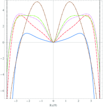
(a) $\alpha<0$

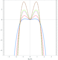
(b) $\alpha>0$

Figure 2: Potential (13) divided by $\epsilon\bar{\rho}$, versus $\text{Re}(\Psi)$ in units of $\sqrt{\bar{\rho}}$, for the following values of $\alpha$: $\pm 0.5$ (solid curve), $\pm 1$ (dashed), $\pm 1.4$ (dash-dotted), $\pm 1.5$ (dash-double-dotted), $\pm 2$ (dash-triple-dotted). Vertical dotted lines represent an infinite well occurring due to the condition $|\Psi|\leqslant|\Psi_{\text{max}}|<\infty$, which follows from the wavefunction’s normalization (2).

III Theory vs experiment

In order to fit the experimental data of Ref. abraham1 , we compare their empirical formulae for an equation of state and a speed of sound with our equations (9) and (10). Since their empirical equation of state is a cubic polynomial, one can immediately deduce that our model must be truncated at a $k=3$ term:

$${\cal N}=3\ \Leftrightarrow\ C_{(k)}=0,\ \forall\,k>3,$$ (11)

and we derive constraints for the remaining coefficients. One can show that those coefficients can be rewritten in the form

$$C_{(\text{ln})}=\alpha^{2},\ C_{(2)}=-\alpha/3,\ C_{(3)}=-1/(2\ 3^{3}),$$ (12)

where $\alpha$ is a real constant, which indicates that the couplings $C_{(\text{ln})}$ and $C_{(2)}$ are not independent from each other, as experimental data suggest. This particular choice of coefficients also ensures that the speed of sound and the pressure difference $P-P_{c}$ share a single common real root in $\bar{\rho}$, as we would anticipate from eq. (1).

Correspondingly, eqs. (4) and (6) become:

$${\cal V}(\rho) = {\cal V}_{(\text{ln})}(\rho)+{\cal V}_{(2)}(\rho)+{\cal V}_{(3)}(\rho),$$ (13)

$${\cal V}_{(\text{ln})}(\rho) = \epsilon\alpha^{2}\rho\left[1-\ln{\left(\rho/\bar{\rho}\right)}\right],$$

$${\cal V}_{(2)}(\rho) = -\frac{1}{3}\epsilon\alpha\bar{\rho}\left(\rho/\bar{\rho}\right)^{2},$$

$${\cal V}_{(3)}(\rho) = -\frac{1}{2\,3^{3}}\epsilon\bar{\rho}\left(\rho/\bar{\rho}\right)^{3},$$

and

$$F(\rho)=-\epsilon\left[\alpha^{2}\ln{(\rho/\bar{\rho})}+\frac{2\alpha}{3}\frac{\rho}{\bar{\rho}}+\frac{1}{18}\frac{\rho^{2}}{\bar{\rho}^{2}}\right].$$ (14)

One can immediately verify that the total many-body potential density (13) is regular in a finite domain, and has a typical Mexican-hat shape which opens either up or down, depending on the sign of $\epsilon$, cf. Fig. 2. This indicates the possibility of spontaneous symmetry breaking, which indeed occurs in the theory of both Gross-Pitaevskii condensates and logarithmic fluids, as discussed in Refs. z11appb ; az11 ; z12eb ; z18epl .

Note that the many-body potentials ${\cal V}_{(2)}$ and ${\cal V}_{(3)}$ can be either repulsive or attractive here, depending on the sign of $\epsilon\alpha$; but the potential ${\cal V}_{(\text{ln})}$ can switch between attractive and repulsive behaviors when the fluid density crosses the value $e\bar{\rho}$, where $e$ being the base of the natural logarithm. This property is essentially the one giving logarithmic fluid the majority of its important features mentioned above.

Figure 3 illustrates how much components ${\cal V}_{(\text{ln})}$, ${\cal V}_{(2)}$ and ${\cal V}_{(3)}$ contribute at different values of density. One can see that the logarithmic component predominates over the polynomial ones for quite a large range of density values, but there is always a threshold density, above which polynomial terms catch up with and overtake the logarithmic term. However, this threshold only exists if its value does not exceed a maximum density value occurring due to the condition $\rho\leqslant|\Psi_{\text{max}}|^{2}<\infty$; the latter follows from eq. (2). The domination of the logarithmic component explains, along with its natural applicability for condensate-like systems z18zna , why the logarithmic fluid is so robust as a leading-order approximation model for a superfluid component of helium II z12eb .

(a) $|\alpha|=1/100$

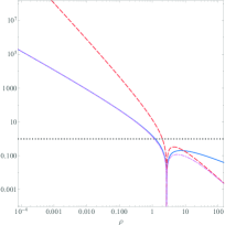
(b) $|\alpha|=1/2$

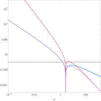
(c) $|\alpha|=1$

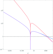
(d) $|\alpha|=100$

Figure 3: Relative values of different terms in a potential (13), versus density in units $\bar{\rho}$: $|{\cal V}_{(\text{ln})}|/|{\cal V}_{(2)}|$ (solid curve), $|{\cal V}_{(\text{ln})}|/|{\cal V}_{(3)}|$ (dashed), and $|{\cal V}_{(\text{ln})}|/|{\cal V}_{(2)}+{\cal V}_{(3)}|$ (dash-dotted). The horizontal dotted line indicates an equality.

Using eqs. (7) - (14), one can easily obtain the equation of state and speed of sound:

$$P\approx P_{c}+\bar{\rho}\,\vartheta^{2}\left(\alpha+\frac{1}{3}\frac{\rho}{\bar{\rho}}\right)^{3}\!,\ c_{s}\approx\vartheta\left(\alpha+\frac{1}{3}\frac{\rho}{\bar{\rho}}\right),$$ (15)

where $\vartheta=\sqrt{\epsilon/m}$ is a characteristic velocity scale.

Note that in the vicinity of its critical pressure point, liquid helium can undergo a cavitation-type phase transition, which is similar to the above-mentioned topological structure transition in logarithmic superfluids. Therefore, the total many-body potential (13) flips, which corresponds to a value $\epsilon$ turning negative. In that case, the speed of sound can formally take imaginary values, which indicates the occurrence of an instability regime.

Furthermore, by eliminating the density $\rho$ from formulae (15), we recover the experimentally measured behaviour of the speed of sound $c_{s}$ in (1) with $\nu={\textstyle\frac{1}{3}}$ where $K=\vartheta/\bar{\rho}$. Moreover, in the case of ⁴He, formulae (15) allow us to assign values to the following combinations of hitherto free parameters:

$$\frac{\vartheta}{\bar{\rho}}=\frac{1}{\bar{\rho}}\sqrt{\frac{\epsilon}{m}}=K=3\sqrt{3}\sqrt{A_{3}},\ \alpha\bar{\rho}=\frac{1}{3}\left(\frac{A_{1}}{A_{2}}-\rho_{0}\right),$$ (16)

where the values of $A$’s and $\rho_{0}$ for ⁴He are given in Refs. abraham1 ; mar94 : $A_{1}=5.6\times 10^{2}$ atm cm³ g^-1, $A_{2}=1.097\times 10^{4}$ atm cm⁶ g^-2, $A_{3}=7.33\times 10^{4}$ atm cm⁹ g^-3, and $\rho_{0}=0.14513$ g cm^-3, while $\alpha$ remains an unfixed dimensionless parameter of the model. This means that our model still has some flexibility left, because $\alpha$ can be used to fit our model for other experiments if necessary. In this paper, $\alpha$ can be set to any negative number, which reflects a scale nature of the parameter $\bar{\rho}$.

We therefore obtain $\vartheta=-4.27\,\alpha^{-1}\times 10^{4}$ $\text{cm}\,\text{s}^{-1}$ and $\bar{\rho}=-\frac{1}{3\alpha}\rho_{c}\approx-3.01\,\alpha^{-1}\times 10^{-2}\,\text{g}\,\text{cm}^{-3}$, where $\rho_{c}$ is the density corresponding to the critical negative pressure $P_{c}$; thus, the ratio $\vartheta/\bar{\rho}=K\approx 1.41\times 10^{6}$ $\text{cm}^{4}\,\text{g}^{-1}\,\text{s}^{-1}$ does not depend on $\alpha$. These numerical values finalize the fitting of the model (3), (13) for the case of ⁴He; the case of bosonized liquid ³He can be done by analogy.

IV Conclusion

A fundamental sound velocity pressure dependence holding up for superfluid helium at low temperatures was examined in the context of the nonlinear wave equation approach for a fluid’s wavefunction. We demonstrated that to explain this dependence, one has to view liquid helium as a mixture of three quantum Bose liquids: a dilute (Gross-Pitaevskii-type) Bose-Einstein condensate, a Ginzburg-Sobyanin-type fluid, and a logarithmic superfluid, where the latter two components can occur due to topological and non-perturbative quantum effects, Efimov trimer states, and fermionic admixtures.

Consequently, the dynamics of such systems is described by a quantum wave equation, which contains both the polynomial (cubic and quintic) nonlinearities with respect to a condensate wavefunction, and an essential non-polynomial logarithmic nonlinearity. Using the hydrodynamic representation of Schrödinger-type equations and experimental data by Abraham et al., we constrained the hitherto free parameters of this multi-component fluid model, and theoretically reproduced the empirical formulae for an equation of state and speed of sound.

- (1) W. M. Whitney and C. E. Chase, Phys. Rev. Lett. 9, 243 (1962)
- (2) W. M. Whitney and C. E. Chase, Phys. Rev. 158, 200 (1967)
- (3) B. M. Abraham, Y. Eckstein, J. B. Ketterson, M. Kuchnir, and P. R. Roach, Phys. Rev. A 1, 250-257 (1970)
- (4) B. M. Abraham, D. Chung, Y. Eckstein, J. B. Ketterson, and P. R. Roach, J. Low Temp. Phys. 6, 521-528 (1972)
- (5) H. Maris, Phys. Rev. Lett. 66, 45 (1991)
- (6) H. Maris, J. Low Temp. Phys. 94, 125 (1994)
- (7) H. Maris, J. Low Temp. Phys. 98, 403-424 (1995)
- (8) A. Qu, A. Trimeche, J. Dupont-Roc, J. Grucker, and Ph. Jacquier, Phys. Rev. B 91, 214115 (2015)
- (9) G. H. Bauer, D. M. Ceperley, and N. Goldenfeld, Phys. Rev. B 61, 9055–9060 (2000)
- (10) F. Dalfovo, A. Lastri, L. Pricaupenko, S. Stringari, and J. Treiner, Phys. Rev. B 52, 1193–1209 (1995)
- (11) J. Boronat, J. Casulleras, and J. Navarro, Phys. Rev. B 50, 3427–3430 (1994)
- (12) H. Maris and D. O. Edwards, J. Low Temp. Phys. 129, 1 (2002)
- (13) I. N. Adamenko, K. E. Nemchenko and I. V. Tanatarov, Phys. Rev. B 67, 104513 (2003)
- (14) V. L. Ginzburg and A. A. Sobyanin, Sov. Phys. Usp. 19, 773 (1976)
- (15) V. L. Ginzburg and A. A. Sobyanin, J. Low Temp. Phys. 49, 507 (1982)
- (16) C. Josserand, Y. Pomeau, and S. Rica, Phys. Rev. Lett. 75, 3150 (1995)
- (17) G. Rosen, J. Math. Phys. 9, 996 (1968)
- (18) G. Rosen, Phys. Rev. 183, 1186 (1969)
- (19) I. Bialynicki-Birula and J. Mycielski, Ann. Phys. (N. Y.) 100, 62 (1976)
- (20) K. Enqvist and J. McDonald, Phys. Lett. B 425, 309-321 (1998)
- (21) K. G. Zloshchastiev, Grav. Cosmol. 16, 288 (2010)
- (22) K. G. Zloshchastiev, Acta Phys. Polon. 42, 261 (2011)
- (23) V. Dzhunushaliev and K. G. Zloshchastiev, Central Eur. J. Phys. 11, 325 (2013)
- (24) T. C. Scott, X. Zhang, R. B. Mann, and G. J. Fee, Phys. Rev. D 93, 084017 (2016)
- (25) V. Dzhunushaliev, A. Makhmudov, and K. G. Zloshchastiev, Phys. Rev. D 94, 096012 (2016)
- (26) T. C. Scott and J. Shertzer, J. Phys. Commun. 2, 075014 (2018)
- (27) A. V. Avdeenkov and K. G. Zloshchastiev, J. Phys. B: At. Mol. Opt. Phys. 44, 195303 (2011)
- (28) K. G. Zloshchastiev, Eur. Phys. J. B 85, 273 (2012)
- (29) B. Bouharia, Mod. Phys. Lett. B 29, 1450260 (2015)
- (30) K. G. Zloshchastiev, Z. Naturforsch. A 72, 677 (2017)
- (31) K. G. Zloshchastiev, Z. Naturforsch. A 73, 619 (2018)
- (32) S. De Martino, M. Falanga, C. Godano, and G. Lauro, Europhys. Lett. 63, 472 (2003)
- (33) G. Lauro, Geophys. Astrophys. Fluid Dyn. 102, 373 (2008)
- (34) K. G. Zloshchastiev, Europhys. Lett. (EPL) 122, 39001 (2018)
- (35) E. P. Gross, Nuov. Cim. 20, 454–457 (1961)
- (36) L. P. Pitaevskii, Sov. Phys. JETP 13, 451 (1961)
- (37) V. Efimov, Sov. J. Nucl. Phys. 12, 589 (1971)
- (38) V. Efimov, Nucl. Phys. A 210, 157 (1973)
- (39) E. A. Kolganova, A. K. Motovilov, and W. Sandhas, Few-Body Syst. 51, 249-257 (2011)
- (40) S. T. Chui and V. N. Ryzhov, Phys. Rev. A 69, 043607 (2004)
- (41) S. T. Chui, V. N. Ryzhov, and E. E. Tareyeva, JETP Lett. 80, 274–279 (2004)
- (42) E. B. Kolomeisky and J. P. Straley, Phys. Rev. B 46, 11749 (1992)
- (43) K. G. Zloshchastiev, J. Theor. Appl. Mech. 57, 843-852 (2019)