Stick-slip and convergence of feedback-controlled systems with Coulomb friction

Abstract

[Summary]An analysis of stick-slip behavior and convergence of trajectories in the feedback-controlled motion systems with discontinuous Coulomb friction is provided. A closed-form parameter-dependent stiction region, around an invariant equilibrium set, is proved to be always reachable and globally attractive. It is shown that only asymptotic convergence can be achieved, with at least one but mostly an infinite number of consecutive stick-slip cycles, independent of the initial conditions. Theoretical developments are supported by a number of numerical results with dedicated convergence examples.

1 Introduction

Feedback-controlled motion systems are mostly subject to nonlinear friction, and the direction-dependent Coulomb friction force plays a crucial role owing to a (theoretical) discontinuity at velocity zero-crossings. Although the more complex dynamic friction laws (see, e.g., ^{5, 6, 1} and references therein) allow the frictional discontinuity to be bypassed during analysis, the basic Coulomb friction phenomenon continues to represent the same challenges in terms of a controller convergence, especially in the presence of an integral control action. An associated stick-slip behavior and so-called frictional limit cycles were formerly addressed in ⁴. An algebraic prediction of stick-slip, with a large set of parametric equalities, was compared to the describing function method, while the Coulomb plus static friction law was assumed for avoiding discontinuity at the velocity zero-crossing. An explicit solution for friction-generated limit cycles has also been proposed in ¹⁹, necessitating static friction approximation (to avoid discontinuity) and also requiring the stiction friction which is larger than the Coulomb friction level. Despite including explicit analysis of state trajectories for both sticking and slipping phases, no straightforward conclusions about the appearance and convergence of stick-slip behavior have been reported. Also several studies on adaptive friction control, correspondingly estimation, attempted formerly to address the nonlinear effects of friction and, correspondingly, compensate for them, see e.g. ⁹. The appearance of friction-induced (so-called hunting) limit cycles has been briefly addressed in ¹⁴, for the assumed LuGre ¹¹ and so-called switch ¹⁶ friction models. Note that before, an earlier analysis of stick-slip behavior and associated friction-induced limit cycles can be found in ²¹. An explanation of how a proportional-feedback-controlled motion with Coulomb friction comes to sticking was subsequently shown in ² by using the invariance principle. Stick-slip behavior, as an observable phenomenon known in the control practice, was highlighted already in ⁵, and several following control studies have since there attempted to analyze and compensate such behaviors. For instance, a related analysis of under-compensation and over-compensation of the static friction was reported in ²⁰. Issues associated with a slow (creeping-like) convergence of the feedback-controlled motion in presence of the Coulomb friction have been addressed and experimentally demonstrated in ²⁴. More recently, the convergence problems of a PID feedback control have been well demonstrated with an accurate experiment in ⁷, while attempting to reduce the settling errors by a reset integral control ¹⁰. The related analysis has been also reported before in ⁸. Despite a number of experimental observations and elaborated studies reported in the literature, it appears that no yet general consensus has been established in relation to the friction-induced stick-slip cycles in the feedback-controlled systems with Coulomb friction. In particular, questions arise over when and under which conditions the stick-slip cycles occur, and how a PID-controlled motion will converge to zero equilibrium in the presence of Coulomb friction, especially with discontinuity. Note that the problem of a slow convergence in vicinity to a set reference position is of particular relevance for the advanced motion control systems, see, e.g., ²⁵. Yet, in the PID design and tuning, see, e.g., ³, the associated issues are not widely accepted and have still to be formalized, this despite a huge demand coming from a precision control engineering. This gap, however, should not come as a fully surprising, given the fact of a nontrivial friction microdynamics (visible from several experimental studies ^{18, 27, 28}), and the uncertain and time-varying friction behavior, see e.g. ²³.

Despite the appearance of the few papers mentioned above, a clearly comprehensible analysis and explanation of the stick-slip behavior due to the integral feedback effect in the presence of Coulomb friction remains underexposed in the system and control literature. The main objective of this paper is in filling this gap. The work is dedicated to the contribution to the convergence analysis of the feedback-controlled systems in the presence of the Coulomb friction and, thus, to the understanding of stick-slip cycles that occur in servomechanisms. The main contributions can be highlighted as following: (i) we derive and describe the closed-form parameter-dependent stiction region encompassing equilibrium region, (ii) we prove that only asymptotic convergence to this region can be achieved and that with stick-slip oscillations. In order to keep the analysis general as possible and to clarify the principal phenomenon of frictional-driven stick-slip response, a classical Coulomb friction law with discontinuity is assumed. This (unavoidably) led to a variable-structure system dynamics, distinguishing between the modes of a motion sticking and slipping. At the same time, we show that all state trajectories always remain continuous and almost always differentiable (except finite switching between both modes). We provide theorems and identify the conditions to demonstrate the sticking region around zero equilibrium to be reachable and globally attractive. The developed analysis is further reinforced by several illustrative numerical examples.

1.1 Problem statement

Throughout the paper, we will deal with the feedback-controlled systems described by

$$\ddot{\phi}(t)+K_{d}\dot{\phi}(t)+K_{p}\phi(t)+K_{i}\int\phi(t)dt+F(t)=0,$$ (1)

where the derivative, proportional and integral feedback gains are $K_{d}$, $K_{p}$ and $K_{i}$, respectively. Note that we are purposefully focusing on a PID-type feedback control (1), where the integral control action is particularly critical for the friction-driven stick-slip effects, as since long known in the control practice. Other types of the feedback controls, still including an integral control action, are also thinkable for analysis but would go far beyond the provided analysis and results. The nonlinear friction (that with discontinuity) is denoted by $F$, and the set-point control problem is reduced to the convergence problem for a non-zero initial condition, i.e., $\phi(0)\neq 0$. Furthermore, we use the following simplifications of the system plant without loss of generality: the relative motion of an inertial body with unity mass is considered in the generalized $(\phi,\dot{\phi})$ coordinates. The inherent system damping (including linear viscous friction) and stiffness (of restoring spring elements) are incorporated (if applicable) into $K_{d}>0$ and $K_{p}>0$, respectively. There are no actuator constraints, so that the feedback of integral output error is directly applicable via the gain factor $K_{i}>0$.

The control problem (1) has long been associated with issues of a slow and/or cyclic convergence of $\phi(t)$ in the vicinity of steady-state for the set-point reference. This (sometimes called hunting behavior or even hunting limit cycles) has been addressed in analysis and also observed in several controlled positioning experiments, e.g., ^{5, 4, 19, 14, 24, 7}. The phenomena seem to be associated with an integral control action and nonlinear (Coulomb-type) friction within a vanishing region around the equilibria, where the potential field of proportional feedback weakens and cannot provide $\phi(t)\rightarrow 0$ within the certain application-required time $t<\mathrm{const}$. The hunting behavior is directly cognate with stick-slip, where a smooth (continuous) motion alternates with a sticking phase of zero or slowly creeping displacement. Stick-slip appearance, parametric conditions, and convergence in semi-stable limit cycles are the focus of our study, while we assume the Coulomb friction force with discontinuity.

2 Stiction due to discontinuous Coulomb friction

In this Section, we analyze the stick-slip behavior of the (1) system, for which the classical Coulomb friction with discontinuity is represented by $F(\dot{\phi})=F_{c}\,\mathrm{sign}(\dot{\phi})$. Here, the Coulomb friction coefficient is $F_{c}>0$, and the sign operator is defined by

$$\mathrm{sign}(z)=\left\{\begin{array}[]{ll}1,&\;z>0,\\ \left[1,1\right],&\;z=0,\\ -1,&\;z<0.\\ \end{array}\right.$$ (2)

Note that (2) constitutes an ideal relay with instantaneous switching upon change of the input sign. We also note that for a zero-displacement rate, the friction equation becomes an inclusion $F(0)\in[-F_{c},F_{c}]$ in the Filippov sense ¹³, when one is seeking for the corresponding analytic solution.

We will consider the feedback-controlled system in a minimal state-space representation as follows:

$$\dot{x} = Ax+Bu,$$ (3)

$$y = Cx,$$ (4)

$$u = -\mathrm{sign}(y).$$ (5)

Note that in this way, we also approach the system notation provided in ¹⁵ for analysis of the relay feedback systems (RFSs). Introducing the state vector $x=(x_{1},x_{2},x_{3})^{T}\in\mathbb{R}^{3}$ of the integral, output, and derivative errors, (1) can be rewritten as (3)-(5), with the system matrix

$$A=\left(\begin{array}[]{ccc}0&1&0\\ 0&0&1\\ -K_{i}&-K_{p}&-K_{d}\\ \end{array}\right),$$ (6)

and input and output distribution vectors

$$B=\left(\begin{array}[]{c}0\\ 0\\ F_{c}\\ \end{array}\right),\quad C^{T}=\left(\begin{array}[]{c}0\\ 0\\ 1\\ \end{array}\right)$$ (7)

correspondingly.

2.1 Without integral feedback

Firstly, we consider the system (3)-(7) without an integral feedback action, meaning $K_{i}=0$. In this case, the phase-plane $(x_{2},x_{3})\in\mathbb{R}^{2}$ is divided into two regions

$$P^{+}=\{x\in\mathbb{R}^{2}:x_{3}>0\},\quad P^{-}=\{x\in\mathbb{R}^{2}:x_{3}<0\}$$ (8)

by the discontinuity manifold $S=\{x\in\mathbb{R}^{2}:x_{3}=0\}$. It can be seen that in the discontinuity manifold $S$, the vector fields of the state value $x_{s}$ are given by

$$f^{+}(x_{s}) =\overset{x\in P^{+}}{\underset{x\rightarrow x_{s}}{\lim}}(Ax+Bu)=\left(\begin{array}[]{c}0\\ -K_{p}x_{2}-F_{c}\end{array}\right),$$ (11)

$$f^{-}(x_{s}) =\overset{x\in P^{-}}{\underset{x\rightarrow x_{s}}{\lim}}(Ax+Bu)=\left(\begin{array}[]{c}0\\ -K_{p}x_{2}+F_{c}\end{array}\right),$$ (14)

and are pointing in the opposite directions within $|x_{2}|\leq F_{c}K_{p}^{-1}$. On the contrary, outside of this region (denoted by $S_{0}$ in Figure 1), both vector fields are pointing in the same direction, towards $P^{+}$ for $x_{2}<-F_{c}K_{p}^{-1}$ and towards $P^{-}$ for $x_{2}>F_{c}K_{p}^{-1}$.

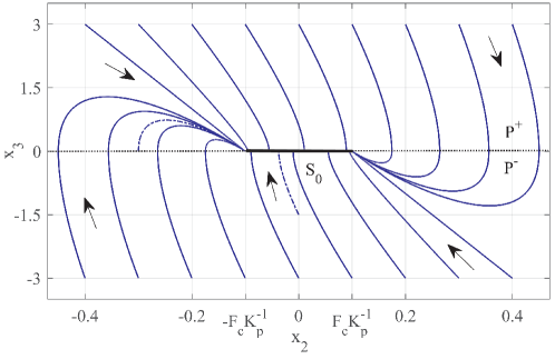
Figure 1: Phase portrait of $(x_{2},x_{3})$-trajectories of the (3)-(7) system without integral feedback, attracted to $S_{0}$ from various initial values

Since both vector fields are normal to the manifold $S$, neither smooth motion nor sliding mode can occur for the $(x_{2},x_{3})\in S_{0}$ trajectories. It means that any trajectory reaching $S_{0}$ will remain there $\forall\>t\rightarrow\infty$. Therefore, $S_{0}$ constitutes the largest invariant set of equilibrium points, for (3)-(7) without integral control action. Note that this has also been shown in ² and is well known when a relative motion with Coulomb friction is controlled by the proportional-derivative (PD) feedback only. In this case, the set value error can be reduced by increasing $K_{p}$ but cannot be driven to zero as long as $F_{c}\neq 0$. The phase portraits of the trajectories converging to $S_{0}$ are exemplary shown in Figure 1 and marked with arrows.

2.2 With integral feedback

When allowing for $K_{i}\neq 0$, it is intuitively apparent that having reached a point $x(t_{s})\in S_{0}$ at $t=t_{s}$, the trajectory cannot remain there for all times $t_{s}<t<\infty$. While the motion states $x_{3}(t_{s})=0$ and $x_{2}(t_{s})=\mathrm{const}\neq 0$, the integral control effort $K_{i}x_{2}(t_{s})\int^{t}_{t_{s}}dt$ grows continuously and, at some finite time ($t_{c}>t_{s}$), will lead to the breakaway ²² and a new onset of a continuous motion. This alternating phase, upon the system sticking, is often referred to as slipping, cf., e.g., ¹⁹, so that a stick-slip motion ^{5, 1} appears also in form of the limit cycles. In order to analyze the friction-induced limit cycles, sometimes denoted as hunting-limit cycles, cf. ¹⁴, we firstly need to look into the system dynamics during the system stiction, i.e., for $t_{s}<t<t_{c}$. Here we recall that during a stiction phase, the system (3)-(7) produces a continuous switching (with infinite frequency) once $x_{3}=0$, this owing to the discontinuous relay nonlinearity (2) which is acting in the feedback loop. One can also notice, in upfront, that for $x_{3}=0$ the solution of (3)-(7) is needed to be specified in the Filippov sense ¹³. Further we note that the below given developments are motivated by analysis of existence of the fast switches provided in ¹⁵ for RFS, while the obtained original results rely on the sliding-mode principles, see, e.g., ^{12, 26}.

Consider the switching variable (or more generally surface) $S=Cx(t)=0$, for which the sliding mode should occur on the manifold $S$. This requires that the existence and reachability condition, cf. ¹²,

$$\dot{S}S\leq-\eta|S|$$ (15)

is fulfilled, where $\eta$ is a small positive constant.

Theorem 2.1.

Given is the control system (3)-(7) with the Coulomb friction. The system is sticking at $x_{3}=0$ iff

$$|K_{i}x_{1}|+|K_{p}x_{2}|\leq F_{c}.$$ (16)

Proof 2.2.

The system remains sticking as long as it is in the sliding mode for which (15) is fulfilled. The sliding-mode condition (15) can be rewritten as

$$\dot{S}\,\mathrm{sign}(S)\leq-\eta,$$ (17)

while the time derivative of the sliding surface is

$$\dot{S}=(CAx\pm CB)=\bigl{(}CAx-\mathrm{sign}(S)CB\bigr{)},$$ (18)

depending on the sign of $Cx$. Substituting (18) into (17) results in

$$CAx \leq CB-\eta\qquad\hbox{for}\quad\mathrm{sign}(S)>0,$$ (19)

$$-CAx \leq CB-\eta\qquad\hbox{for}\quad\mathrm{sign}(S)<0.$$ (20)

Since $CB,\eta>0$, the inequalities (19) and (20) can be summarized in

$$|CAx|\leq CB-\eta.$$ (21)

Evaluating (21) with $x_{3}=0$ and $0\neq\eta\rightarrow 0^{+}$ results in (16) and completes the proof.

Remark 2.3.

The condition obtained by the Theorem 2.1 is equivalent to the set of attraction $\{x\in S:|CAx|<|CB|\}$ for $CB>0$ that was demonstrated in ¹⁵ Section 4.

Now, we are interested in the state dynamics during the system stiction, which means within the sliding mode. Since staying in the sliding mode (correspondingly on the switching surface $S\equiv 0$) requires

$$\dot{S}=C\dot{x}=CAx+CBu=0\qquad\hbox{for}\quad t_{s}<t<t_{c},$$ (22)

one obtains the so-called equivalent control as

$$u_{e}=-(CB)^{-1}CAx.$$ (23)

Recall that an equivalent control, ²⁶, is the linear one (i.e. without a relay action) which is required to maintain the system in an ideal sliding mode without fast-switching. Consequently, substituting (23) into (3) results in the equivalent system dynamics

$$\dot{x}_{e}=\bigl{[}I-B(CB)^{-1}C\bigr{]}Ax_{e}=OAx_{e},$$ (24)

which governs the state trajectories as long as the system remains in the sliding mode, and where $x_{e}=(x_{1},x_{2},0)^{T}$. Here $O$ is the so-called projection operator of the original system dynamics, satisfying the properties $CO=0$ and $OB=0$. Evaluating (24) with (6) and (7) yields the equivalent system dynamics during the stiction as

$$\left(\begin{array}[]{c}\dot{x}_{1}\\ \dot{x}_{2}\\ \dot{x}_{3}\\ \end{array}\right)=\left(\begin{array}[]{ccc}0&1&0\\ 0&0&1\\ 0&0&0\\ \end{array}\right)\left(\begin{array}[]{c}x_{1}(t_{s})\\ x_{2}(t_{s})\\ 0\\ \end{array}\right).$$ (25)

It can be seen that neither relative displacement nor its rate will change when the system is sticking, although the integral error grows according to

$$x_{1}(t)=x_{1}(t_{s})+x_{2}(t_{s})\int\limits^{t_{c}}_{t_{s}}dt.$$ (26)

Further it can be noted that if $K_{i}=0$ then the condition (16), correspondingly the inequality $|CAx|\leq|CB|$, reduces to $|x_{2}|\leq F_{c}K_{p}^{-1}$, while the sliding mode (25) reduces to the zero dynamics of the system in stiction (cf. with results in Section 2.1).

2.3 Region of attraction

Theorem 2.1 provides the necessary and sufficient condition for the system (3)-(7) remains sticking. Yet it is also necessary to demonstrate the global attraction of state trajectories to the stiction region. Recall that the latter corresponds to the subset

$$S_{0}=\{x\in\mathbb{R}^{3}\,:\,x_{3}=0,\,|K_{i}x_{1}|+|K_{p}x_{2}|\leq F_{c}\}$$ (27)

where the sliding mode occurs (cf. (16) and (25)).

Firstly, we will explore the persistence of the sliding mode, meaning we will prove whether the system can stay incessantly inside of $S_{0}^{s}=\{S_{0}\,:\,x_{2}\neq 0\}$, i.e., for all times $t_{s}<t\rightarrow\infty$. By making $(x_{1},x_{2})$-projection of $x\in\mathbb{R}^{3}$, one can show that (16) results in a rhombus, as schematically illustrated in Figure 2.

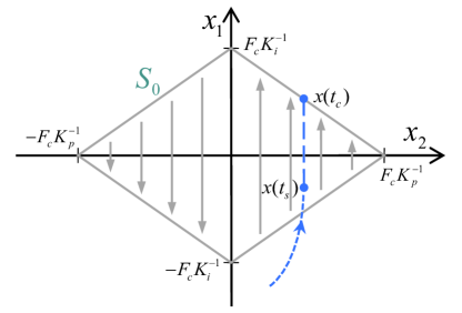
Figure 2: Rhombus-shape, in $(x_{1},x_{2})$-projection, of the $S_{0}$-region of attraction, with vector-field during the stiction mode and example of an entering and leaving trajectory at $t_{s}$ and $t_{c}$, respectively

The indicated vector field is unambiguous due to the integral control action (cf. the sliding-mode dynamics (25)). It means that after reaching $S_{0}^{s}$ at $t_{s}$, any trajectory will leave it at $t_{c}$ once it hits the boundary of $S_{0}$. Denoting the point of reaching $S_{0}^{s}$ by $x(t_{s})\equiv(x^{s}_{1},x^{s}_{2},0)$, one can calculate the new point of leaving $S_{0}^{s}$ as

$$x_{1}(t_{c})=:x^{c}_{1}=x^{s}_{2}\bigl{(}F_{c}|x^{s}_{2}|^{-1}-K_{p}\bigr{)}K^{-1}_{i}.$$ (28)

Correspondingly, from (26) and (28) one obtains the time of leaving $S_{0}^{s}$ as

$$t_{c}=\Bigl{[}x^{s}_{2}\bigl{(}F_{c}|x^{s}_{2}|^{-1}-K_{p}\bigr{)}K^{-1}_{i}-x^{s}_{1}+x^{s}_{2}t_{s}\Bigr{]}(x^{s}_{2})^{-1}.$$ (29)

From the above, it can be recognized that if $K_{i}\rightarrow 0$, the stiction region $S_{0}$ blows to the entire $(x_{1},x_{2})$-subspace and, consequently, $t_{c}\rightarrow\infty$. It means that a system trajectory will never leave $S_{0}$ having reached it – the result which is fully in line with what was demonstrated in Section 2.1. On other hand, if allowing for $K_{i}\rightarrow\infty$ the time instant $t_{c}\rightarrow t^{+}_{s}$, according to (29) with $x^{s}_{1}\rightarrow 0$, due to $S_{0}$ is collapsing to $\mathrm{proj}_{x_{2}}S_{0}$.

Let us now demonstrate that $S_{0}$ is globally attractive for all initial values outside of $S_{0}$, meaning $\forall\>x(t_{0})\in\mathbb{R}^{3}\backslash S_{0}$. Using the eigen-dynamics of (3) with (6), which are linear, one can ensure the global exponential stability by analyzing the characteristic polynomial

$$s^{3}+K_{d}s^{2}+K_{p}s+K_{i}=0$$ (30)

and applying the standard Routh-Hurwitz stability criterion. Then, the control parameters condition

$$K_{d}K_{p}>K_{i}$$ (31)

should then be satisfied, for guaranteeing that all eigenvalues $\lambda_{i}$ of the system matrix (6) have $\mathrm{Re}\{\lambda_{i}\}<0$ with $i=1,\ldots,3$. Then, the resulting (switched) subsystems $\dot{x}=Ax\mp B$ behave as asymptotically stable in both subspaces $\{x\in\mathbb{R}^{3}\backslash S_{0}:x_{3}\gtrless 0\}$ correspondingly. It should be noted that the condition of the above parameters is conservative, since the Coulomb friction itself is always dissipative, independently of whether $x_{3}>0$ or $x_{3}<0$. This can be shown by considering the dissipated energy

$$\bar{V}(t)=-F(t)\int\dot{\phi}(t)dt=-F(t)\bar{\phi},$$ (32)

which is equivalent to a mechanical work provided by the constant friction force $F$ along an unidirectional displacement $\bar{\phi}$. Taking the time derivative of (32) and substituting the Coulomb friction law results in

$$\frac{d}{dt}\bar{V}(t) = -\frac{d}{dt}F(t)\bar{\phi}-F(t)\frac{d}{dt}\bar{\phi}$$ (33)

$$= 0-F_{c}\mathrm{sign}\bigl{(}\dot{\phi}(t)\bigr{)}\dot{\phi}(t)=-F_{c}\bigl{|}\dot{\phi}(t)\bigr{|}.$$

Therefore, $\dot{\bar{V}}(t)<0$ for all $x_{3}(t)\neq 0$. This quite intuitive, yet relevant to be analytically expressed, condition reveals the relay feedback (5) as an additional (rate-independent) damping, which contributes to stabilization of the closed-loop dynamics (3)-(7). This result will be further used for the proof of Corollary 2.4. Notwithstanding this additional stabilizing by-effect, we will keep the conservative stability condition (31) as the sufficient (but not necessary) one. This appears reasonable due to an usually uncertain Coulomb friction coefficient and, hence, in order for increasing the overall robustness of the feedback control system. The following example should, however, exemplify the additionally stabilizing behavior of the Coulomb friction, even when (31) is violated.

Consider the system (3)-(7) with $K_{d}=0$, $K_{p}=100$ and $K_{i}=1$. The eigenvalues of the system matrix $A$ are $\lambda_{1}=-0.01$, $\lambda_{2,3}=0.0005\pm 10j$, which implies the linear subsystem is asymptotically unstable. It should also be noted that (31) is not fulfilled. To evaluate the trajectories of the system (3)-(7), one can use the particular solution

$$x(t)=e^{At}x(\tau)+A^{-1}\bigl{(}e^{At}-I\bigr{)}Bu,$$ (34)

for the constant control $u=\mp 1$, which corresponds to the relay (5), switched in the $x_{3}>0$ and $x_{3}<0$ subspaces. The initial values $x(\tau)=[x_{1}(t),x_{2}(t),0]^{T}$ at $t=\tau$ should be reassigned each time the trajectory crosses the $(x_{1},x_{2})$-plane, meaning the relay switches at $x_{3}=0$ outside of $S_{0}$. The $x_{3}$-state trajectory, with an initial value $x_{3}(0)=10$, is shown in Figure 3, once for $F_{c}=0$ (solid red line) and once for $F_{c}=1$ (blue dash-dot line).

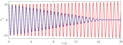
Figure 3: Velocity trajectories (from $x_{3}(0)=10$) of the Example 2.3 system with $F_{c}=0$ (solid red line) and $F_{c}=1$ (blue dash-dot line)

It is easy to recognize that even a low-valued Coulomb friction coefficient ($F_{c}=1$ compared to the proportional feedback gain $K_{p}=100$) leads to a stabilization of the, otherwise, unstable closed-loop control response.

Corollary 2.4.

Consider the system (3)-(7) with the control parameters satisfying (31). The stiction region (27), given by the Theorem 2.1, is globally attractive for all initial values outside of this region, i.e. for all $x(t_{0})\in\mathbb{R}^{3}\backslash S_{0}$.

Proof 2.5.

By virtue of the passivity theorem, e.g., ^{29, 17}, the feedback interconnection of the energy dissipating systems is also energy dissipating. Since (3), (4) is dissipative when (31) is fulfilled, and (5) is also dissipative for $x_{3}\neq 0$, their feedback interconnection yields dissipative almost everywhere (except $x_{3}=0$) outside of $S_{0}$. This implies that any $x(t)$-trajectory, starting from outside of $S_{0}$, converges continuously, and some ball $\mathcal{B}\equiv\|x\|$ around the origin shrinks over time:

$$\|x(t_{2})\|<\|x(t_{1})\|\quad\forall\quad t_{2}>t_{1},\>x\in\mathbb{R}^{3}\backslash S_{0}.$$ (35)

For some $t_{3}>t_{2}$, the shrinking circle becomes $\mathrm{proj}_{(x_{1},x_{2})}\mathcal{B}\subseteq S_{0}$, and for $t_{4}\geq t_{3}$ a zero velocity $x_{3}(t_{4})=0$ will be consequently reached. This implies $x(t_{4})\in S_{0}$, which completes the proof.

Remark 2.6.

The sliding-mode condition (17), which results in $|CAx|\leq CB$ and proves the Theorem 2.1, correspondingly, constitutes the existence and reachability condition for $S_{0}$, and is necessary but not sufficient. This is because (16) does not contain any requirements imposed on the $K_{d}$-parameter value. Theorem 2.1 and Corollary 2.4 constitute the necessary and sufficient conditions for $S_{0}$ to be both – the globally reachable and attractive from outside of $S_{0}$.

3 Analysis of stick-slip convergence

In this Section, we will analyze the convergence behavior of stick-slip trajectories of the system (3)-(7). Recall that having reached $S_{0}^{s}$ at $t_{s}$, the $x(t)$ trajectory will leave it at $t_{c}$, given by (29), which is due to the growing $|x_{1}(t)|$ value, that will (unavoidably) violate the stiction condition (16). To show (qualitatively) how the state trajectories evolve during a stick-slip cycle, consider the triple-integrator chain (see Figure 4(a)), which arises out of the closed-loop dynamics (1).

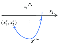
(a)              
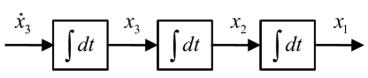
(b) (c)
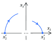
(d)           

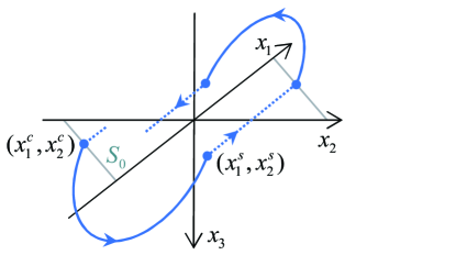
Figure 4: Phase portrait at stick-slip; (a) triple-integrator chain, (b) $(x_{1},x_{2})$-projection during sticking, (c) $(x_{2},x_{3})$-projection during slipping, (d) typical trajectory during one stick-slip cycle

Eliminating the time argument, which is a standard procedure for a phase-plane construction, one can write

$$x_{n}dx_{n}=\dot{x}_{n}dx_{n-1},\quad n=\{3,2\},$$ (36)

in general terms, that for the first and second (from the left to the right) integrator. For an unidirectional motion (here $\mathrm{sign}(x_{3})=1$, for instance, is assumed) and piecewise constant approximation $\dot{x}_{n}=\mathrm{const}$, one obtains

$$x_{1} = x^{2}_{2}(2x_{3})^{-1}-x_{1}^{min},$$ (37)

$$x_{2} = x^{2}_{3}(2\dot{x}_{3})^{-1}-x_{2}^{c}$$ (38)

after integrating the left- and right-hand sides of (36). Obviously, for $t\geq t_{c}$, the $x_{1}(t)$-trajectory evolves parabolically, depending from $x_{2}(t)$, see Figures 4(b). The $x_{3}(t)$-trajectory is square-root-dependent of $x_{2}(t)$, see Figures 4(c) correspondingly. Note that the increasing and decreasing segments of the corresponding trajectories are both asymmetric, effectively due to non-constant $\dot{x}_{n}$-value as the motion evolves. At the same time, one can stress that the extremum $x_{1}^{min}$ (here, minimal due to the assumed positive sign of velocity) always lies on the $x_{1}$-axis (cf. Figure 4(b)) owing to $x_{1}=\int x_{2}dt$, and $\mathrm{sign}(x_{3})=\mathrm{const}$. Differently, the $(x_{2},x_{3})$-projection of the $x(t)$-trajectory can be shifted along the $x_{2}$-axis, while it always ends in $x_{3}(t_{s})=0$ for $x(t)\in S_{0}$ (cf. Figure 4(c)). The resulting alternation of the stick-slip phases is schematically shown in Figure 4(d).

Proposition 3.1.

Having reached $S_{0}$, the system (3)-(7) does not leave $\Omega\in\mathbb{R}^{3}$ with $\mathrm{proj}_{(x_{1},x_{2})}\Omega\subseteq S_{0}$ and converges asymptotically to $x(t)\underset{t\rightarrow\infty}{=}\bigl{\{}(x_{1},0,0):\,|x_{1}|\leq F_{c}K_{i}^{-1}\bigr{\}}$ within multiple (or at least one) stick-slip cycles. The stick-slip cycles can occur with either zero-crossing of $x_{2}$ or with keeping the same $\mathrm{sign}(x_{2}(t_{s,1}))$, where $t_{s,1}$ is the time instant when $x(t)$ reaches $S_{0}$ for the first time.

When first disregarding the frictional side-effect, i.e., $F_{c}=0$, it is well understood that a non-overshoot of the set reference value cannot be reached, independently of the assigned control parameters, provided (i) $K_{i}\neq 0$ and (ii) the initial conditions are such that either $x_{1}(0)=0$ or $\mathrm{sign}(x_{1}(0))=\mathrm{sign}(x_{2}(0))$. This becomes evident since the integral error state $x_{1}(t)$ accumulates the output error over time. That is, in order for the $|x_{1}(t)|$ starts to decrease, at least one change of the $x_{2}(t)$-sign is required. An exception is when $\mathrm{sign}(x_{1}(0))\neq\mathrm{sign}(x_{2}(0))$, which allows both $x_{1}(t)$ and $x_{2}(t)$ to converge to zero from the opposite directions. Thus, at least one overshoot should appear, even if all control gains are assigned to have the real poles only; see later the Example 4.

When the Coulomb friction becomes effective, i.e., $F_{c}\neq 0$, the system can change to the stiction again, and that also without overshoot of $x_{2}=0$, after starting to slip at $x(t_{c})$. It means that a motion trajectory lands again onto $S_{0}$ at time $t_{s,2}>t_{c}>t_{s,1}$ and that with $\mathrm{sign}(x_{2}(t_{s,2}))=\mathrm{sign}(x_{2}(t_{s,1}))$. Since the system with $K_{d},F_{c}>0$ is dissipative, the energy level is $V(t_{s,2})<V(t_{c})$, meaning the motion trajectory $x(t)$ always lands onto $S_{0}$ closer to the origin than it was when leaving $S_{0}$ in $x(t_{c})$. Note that the system energy within $S_{0}$ can be expressed by the potential field of the proportional and integral control errors, yielding

$$V(t)=\frac{1}{2}K_{i}x_{1}^{2}+\frac{1}{2}K_{p}x_{2}^{2}\quad\hbox{for}\quad t\in[t_{s},\ldots,t_{c}].$$ (39)

One can recognize that the energy level (39), of the system in stiction, is an ellipse

$$\frac{x_{2}^{2}}{a^{2}}+\frac{x_{1}^{2}}{b^{2}}=1\quad\hbox{with}\quad a^{2}=2VK_{p}^{-1},\;b^{2}=2VK_{i}^{-1}.$$ (40)

Since the energy $V(t_{c})$ is bounded by $S_{0}$, cf. Figure 2, one can show that the semi-major axis is $a\leq F_{c}K_{p}^{-1}$ and the semi-minor axis is $b\leq F_{c}K_{i}^{-1}$. From the system dissipativity and global attractiveness of $S_{0}$, cf. Corollary 2.4, it follows that the trajectory becomes sticking again, meaning $x(t)\in S_{0}$ for $t\geq t_{s,2}>t_{c}$. Since $V(t_{s,2})<V(t_{c})$, the ellipse (40) shrinks as $a$ and $b$ become smaller; note that both are proportional to $V(t)$. It is important to notice that during the system is sticking, the energy level increases, on the contrary, since $V(t_{c})>V(t_{s,1})$. This is consequently logical since the integral control action feed an additional energy into the control loop when the system is at a standstill. That leads to a breakaway and allows for the motion to restart again once the sticking trajectory reaches the $S_{0}$-boundary.

Remark 3.2.

When the state trajectory reattains the stiction region $x(t_{s,2})\in S_{0}$ without overshoot, meaning $\mathrm{sign}(x_{2}(t_{s,2}))=\mathrm{sign}(x_{2}(t_{c}))$, the system is over-damped by the Coulomb friction. Otherwise, $\mathrm{sign}(x_{2}(t_{s,2}))\neq\mathrm{sign}(x_{2}(t_{c}))$ means the system is said to be under-damped by the Coulomb friction. A special, but as will be shown not feasible, case of $x_{2}(t_{s,2})=0$, meaning the system reaches equilibrium $S_{0}\backslash S_{0}^{s}$ and remains there $\forall\>t\geq t_{s,2}$, is analyzed below by proving the Theorem 3.3.

Theorem 3.3.

The system (3)-(7), with control parameters satisfying (31) and $F_{c}>0$, converges asymptotically to the invariant set $\Lambda=\{(x_{1},0,0):|x_{1}|\leq F_{c}K_{i}^{-1}\}$ during a number of stick-slip cycles $N\in\mathbb{N}$, with $1\leq N<\infty$. And there are no system parameter values and stick-slip initial conditions $(x_{1}(t_{s,n}),x_{2}(t_{s,n}))$ with $n<N$ which allow the trajectory to reach $\Lambda$ at the end of the next following stick-slip cycle within the time $t_{s,n+1}>t_{c,n}>t_{s,n}$.

Proof 3.4.

The convergence to $\Lambda$ follows from system the dissipativity during the slipping and, correspondingly, shrinking ellipse (40), which implies an always decreasing energy level by the end of one stick-slip cycle, i.e. $V(t_{s,n+1})<V(t_{s,n})$. This implies $|x_{2}(t_{s,n+1})|<|x_{2}(t_{s,n})|$ for $n\in N$ and ensures such $x(t)$-trajectories which start slipping at $t_{c,n}$ and land closer to the origin at $t_{s,n+1}$ than before at $t_{s,n}$.

The proof of the second part of the Theorem 3.3, which says it is impossible to reach the invariant equilibrium set $\Lambda$ after one particular stick-slip cycle, follows through the contradiction. For this purpose, we should first assume that there is a particular setting $\bigl{(}K_{p},K_{i},K_{d},F_{c},x_{1}(t_{s,n}),x_{2}(t_{s,n})\bigr{)}$ for which the state trajectory $x(t_{s,n+1})\in\Lambda$, i.e. in the next stiction phase at the finite time $t_{s,n+1}>t_{c,n}>t_{s,n}$. The initial conditions of a slipping phase are always given, cf. with Section 2.3, by

$$x_{2}(t_{c,n}) = x_{2}(t_{s,n}),$$ (41)

$$x_{1}(t_{c,n}) = \frac{F_{c}}{K_{i}}-\frac{K_{p}}{K_{i}}x_{2}(t_{c,n})\>\hbox{ in 1st quadrant,}$$ (42)

$$x_{1}(t_{c,n}) = -\frac{F_{c}}{K_{i}}-\frac{K_{p}}{K_{i}}x_{2}(t_{c,n})\>\hbox{ in 3rd quadrant}$$ (43)

This becomes apparent when inspecting the stiction phase dynamics (25), (26) and $S_{0}$-boundary, cf. Figure 2. For reaching $\Lambda$ at a final time instant $\psi=t_{s,n+1}$, while starting at $\tau=t_{c,n}$, an explicit particular solution of

$$0=C\Bigl{[}e^{A\psi}\left(\begin{array}[]{c}x_{1}(\tau)\\[-1.42271pt] x_{2}(\tau)\\[-1.42271pt] 0\end{array}\right)+A^{-1}(e^{A\psi}-I)Bu-\left(\begin{array}[]{c}x_{1}(\psi)\\[-1.42271pt] 0\\[-1.42271pt] 0\end{array}\right)\Bigr{]}$$ (44)

with $u=\pm 1$, should exist, cf. with (34). Due to the symmetry of solutions, we will consider the 1st quadrant of $S_{0}$ only, i.e., with the above initial condition (42) and $u=+1$ correspondingly, this without loss of generality when solving (44). Recall that the matrix exponential

$$e^{A\psi}=\sum^{\infty}_{k=0}\frac{(A\psi)^{k}}{k!}$$ (45)

has to be evaluated to find an explicit solution of (44). Substituting the initial conditions, i.e. (41) and (42), into (44) we solve (44) with respect to $x_{2}(\tau)$, and that for an gradually increasing $k=[1,\ldots,40]$. Note that an increasing $k$ provides solely an increased accuracy in evaluating the matrix exponential (45). For all the solutions evaluated with the help of the Symbolic Math Toolbox^TM, it is found that (44) has no initial-value solution other than zero, meaning $x_{2}(\tau)=x_{2}(t_{s,n})=0$. That means there are no other initial conditions than zero for which a stick-slip cycle could lead to $x(t)\in\Lambda$ at $t=t_{s,n+1}$. This contradicts our initial assumption that such initial conditions exist and, hence, completes the proof.

Remark 3.5.

Since no relative motion occurs during a stiction phase, cf. Section 2.2, the trajectory solution (44) represents the single descriptor of the system dynamics, which is determining convergence during the slipping phases. One can recognize that the discontinuous Coulomb friction contributes as a constant piecewise-continuous input $u$ to the solution of trajectories $x(t)$ at $t_{c,n}<t<t_{s,n+1}$. Thus, it comes as not surprising that the stick-slip convergence appears only asymptotically, meaning either within one or a (theoretically) infinite number of the stick-slip cycles. We also note that this is independent of whether $x(t)$ reattains $S_{0}$ with or without overshooting of $x_{2}=0$.

4 Numerical examples

The following numerical examples serve to illustrate and evaluate the above analysis. A dedicated numerical simulation of the stick-slip dynamics is developed by implementing (25), (26) and (34), while the conditions of Theorem 2.1 provide switching between the piecewise smooth trajectories of the alternating slipping and sticking phases of the relative motion of system (3)-(7).

Consider the system (3)-(7) with $K_{d}=20$, $K_{p}=100$, $K_{i}=1000$ and varying $F_{c}=\{50,75,100\}$. The initial values are assigned as $x(0)=\{0,-1.1,0\}$, corresponding to a classical positioning task for the feedback-controlled system (1). Note that $|x_{2}(0)|>F_{c}K_{p}^{-1}$ so that the trajectories start outside of $S_{0}$ and are, therefore, inherently in the slipping phase. The transient and convergence responses for all three Coulomb friction values are shown opposite to each other in Figure 5, cf. qualitatively with an experimental convergence pattern reported in ⁷ Fig 4.

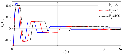
(a) (b)

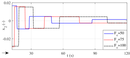
Figure 5: Output response of Example 4: transient phase $t=[0,\ldots,12]$ sec (a), convergence phase $t=[12,\ldots,120]$ sec (b)

Consider the system (3)-(7) with $K_{d}=10$, $K_{p}=1040$, $K_{i}=8000$ and $F_{c}=100$. The initial values $x(0)=(0,-0.15,0)$ are assigned to be close to, but still outside of, the $S_{0}$-region. The linear damping $K_{d}$ is selected with respect to $F_{c}$, so that the system exhibits only one initial overshoot; and the stick and slip phases alternate without changing the sign of $x_{2}$. The output displacement response is shown in Figure 6(a). The stick-slip convergence without zero-crossing is particularly visible on the logarithmic scale in Figure 6(b). Note that after the series of stick-slip cycles, a further evaluation of the alternating dynamics (about $10^{-13}$ in order of magnitude) is no longer feasible, due to a finite time step and corresponding numerical accuracy, cf. 1st quadrant of the $S_{0}$-rhombus in Figure 2.

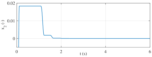
(a) (b)

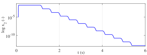
Figure 6: Output (a) and its logarithmic (b) response of Example 4

Consider the system (3)-(7) with $K_{d}=56$, $K_{p}=1040$, $K_{i}=6400$ and $F_{c}=100$. Note that the control gains are assigned in such a way that the linear dynamics (3) and (6) reveal a double real pole at $\lambda_{1,2}=-20$ and the third one in its vicinity at $\lambda_{3}=-16$. This ensures that all states converge fairly simultaneously towards zero, once the $\mathrm{sign}(x_{3})$ remains unchanged. For the initial conditions, $x_{1}(0),x_{3}(0)=0$ and the varying initial displacements $x_{2}(0)=\{-0.2,-0.25,-0.3,-0.35\}$ are assumed. Note that all $x(0)$ are outside of $S_{0}$, while the transient overshoot lands (in all cases) within $S_{0}$, thus directly leading to the first stiction after an overshoot; see Figure 7. One can recognize that the integral state requires, then, the quite different times before the system passes again into the slipping. During the slipping phase, all states converge asymptotically towards zero, provided $F_{c}$ remains constant. Here, it is important to notice that in the real physical systems, a varying $F_{c}$-value and the so-called frictional adhesion, see e.g. ³⁰, at extremely low velocities, will both lead to the system passing into a sticking phase again, therefore, provoking rather the multiple stick-slip cycles. Even though it is not a case here with our ideal Coulomb friction assumption, the Theorem 3.3 still holds, since there is only an asymptotic convergence after at least one stick-slip cycle occurred.

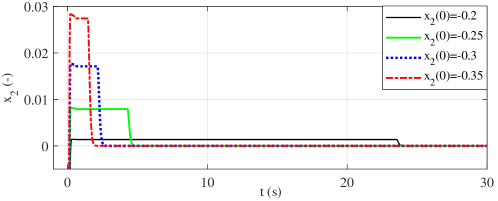
Figure 7: Output response of Example 4 for different initial values

Consider the system (3)-(7) with $K_{d}=20$, $K_{p}=100$, $K_{i}=1000$ and $F_{c}=50$. The initial condition $x(0)=(0,-0.5,0)$ is assigned to be on the boundary of $S_{0}$, thus leading to a short initial slipping and, then, providing a large number of the stick-slip cycles by a long-term simulation with $t=[0,\ldots,100000]$ sec. The output is shown as logarithmic absolute value (due to the alternating sign) over the logarithmic time argument in Figure 8. One can recognize that each consequent sticking phase proceeds closer to the origin, while the stick-slip period grows exponentially, cf. the logarithmic timescale. This further confirms an asymptotic convergence within the stick-slip cycles, cf. Theorem 3.3.

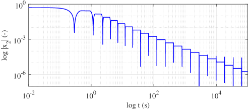
Figure 8: Output response of Example 4, the logarithmic absolute value over the logarithmic time argument

5 Conclusions

An analysis of the stick-slip behavior during settling of the feedback-controlled motion with Coulomb friction has been developed. The most general case of a frictional discontinuity at velocity zero-crossing has been assumed, and the parametric conditions for appearance of a stiction region, encompassing the equilibrium set, have been derived, that independent of the initial conditions.

To notice is that a symmetric Coulomb friction about the origin (i.e. zero velocity) is considered. For an asymmetric friction, i.e. with different Coulomb friction coefficients $F_{c,\{p,n\}}$ for positive (p) and negative (n) direction, the provided analysis is equally valid and requires solely a separate trajectories evaluation for $x_{3}>0$ and $x_{3}<0$, cf. Section 3. The aspects of Stribeck friction (see e.g. ⁵ for details) are not accounted as less relevant for principal stick-slip behavior, even though they certainly affect the period and shape of the corresponding stick-slip cycles. Here we recall that the Stribeck effect provides a short-term transient negative damping and, therefore, rather contributes to the fact that the trajectories each time leave earlier a stiction region, before (unavoidably) coming back into stiction at $x_{2}\neq 0$.

Theorem 2.1 and Corollary 2.4 proved the stiction region to be globally reachable and attractive. Theorem 3.3 stated that the convergence is only asymptotically possible and occurs with at least one but mostly an infinite number of the stick-slip cycles in a sequence. In particular, an ’ideal’ convergence of the control configuration with all real poles in a neighborhood to each other appears with one initial stick-slip cycle, followed by an asymptotic convergence without new stick-slip transitions. The number of illustrative numerical examples, with different initial conditions and parameter settings, argue in favor of the developed analysis and provide additional insight into the stick-slip mechanisms of a feedback controlled motion with Coulomb friction.

Author Biography

Michael Ruderman earned his Dr.-Ing. degree in electrical engineering from TU University Dortmund, Germany, in 2012. He is a full professor at the University of Agder, Grimstad, Norway, teaching control theory in B.Sc., M.Sc., and Ph.D. degree programs. He serves in different editorial boards and technical committees of IEEE and IFAC societies and is chairing IEEE/IES TC on Motion Control in the terms 2018-2019 and 2020-2021. He is a Senior Member of IEEE and was the general chair of the 16th IEEE International Workshop on Advanced Motion Control, in 2020. His current research interests are in motion control, nonlinear dynamics, and hybrid control systems.

References

- 1 F. Al-Bender and J. Swevers, Characterization of friction force dynamics, IEEE Control Systems Magazine 28 (2008), no. 6, 64–81.
- 2 J. Alvarez, I. Orlov, and L. Acho, An invariance principle for discontinuous dynamic systems with application to a Coulomb friction oscillator, J. Dyn. Sys., Meas., Control 122 (2000), no. 4, 687–690.
- 3 K. H. Ang, G. Chong, and Y. Li, PID control system analysis, design, and technology, IEEE transactions on control systems technology 13 (2005), no. 4, 559–576.
- 4 B. Armstrong and B. Amin, PID control in the presence of static friction: A comparison of algebraic and describing function analysis, Automatica 32 (1996), no. 5, 679–692.
- 5 B. Armstrong-Hélouvry, P. Dupont, and C. C. De Wit, A survey of models, analysis tools and compensation methods for the control of machines with friction, Automatica 30 (1994), no. 7, 1083–1138.
- 6 J. Awrejcewicz and P. Olejnik, Analysis of Dynamic Systems With Various Friction Laws, ASME Applied Mechanics Reviews 58 (2005), no. 6, 389–411.
- 7 R. Beerens et al., Reset integral control for improved settling of PID-based motion systems with friction, Automatica 107 (2019), 483–492.
- 8 A. Bisoffi et al., Global asymptotic stability of a PID control system with Coulomb friction, IEEE Transactions on Automatic Control 63 (2017), no. 8, 2654–2661.
- 9 C. Canudas, K. Astrom, and K. Braun, Adaptive friction compensation in dc-motor drives, IEEE Journal on Robotics and Automation 3 (1987), no. 6, 681–685.
- 10 J. Clegg, A nonlinear integrator for servomechanisms, Transactions of the American Institute of Electrical Engineers, Part II: Applications and Industry 77 (1958), no. 1, 41–42.
- 11 C. C. De Wit et al., A new model for control of systems with friction, IEEE Transactions on automatic control 40 (1995), no. 3, 419–425.
- 12 C. Edwards and S. Spurgeon, Sliding mode control: theory and applications, CRC Press, 1998.
- 13 A. Filippov, Differential equations with discontinuous right-hand sides, 1988.
- 14 R. H. Hensen, M. Van de Molengraft, and M. Steinbuch, Friction induced hunting limit cycles: A comparison between the LuGre and switch friction model, Automatica 39 (2003), no. 12, 2131–2137.
- 15 K. H. Johansson, A. Rantzer, and K. J. Åström, Fast switches in relay feedback systems, Automatica 35 (1999), no. 4, 539–552.
- 16 D. Karnopp, Computer simulation of stick-slip friction in mechanical dynamic systems, Journal of dynamic systems, measurement, and control 107 (1985), no. 1, 100–103.
- 17 H. Khalil, Nonlinear Systems, 3rd edn., Prentice Hall, 2002.
- 18 T. Koizumi and H. Shibazaki, A study of the relationships governing starting rolling friction, Wear 93 (1984), no. 3, 281–290.
- 19 H. Olsson and K. J. Astrom, Friction generated limit cycles, IEEE Transactions on Control Systems Technology 9 (2001), no. 4, 629–636.
- 20 D. Putra, H. Nijmeijer, and N. van de Wouw, Analysis of undercompensation and overcompensation of friction in 1DOF mechanical systems, Automatica 43 (2007), no. 8, 1387–1394.
- 21 C. J. Radcliffe and S. C. Southward, A property of stick-slip friction models which promotes limit cycle generation, American Control Conference, 1990, 1198–1205.
- 22 M. Ruderman, On break-away forces in actuated motion systems with nonlinear friction, Mechatronics 44 (2017), 1–5.
- 23 M. Ruderman and M. Iwasaki, Observer of nonlinear friction dynamics for motion control, IEEE Transactions on Industrial Electronics 62 (2015), no. 9, 5941–5949.
- 24 M. Ruderman and M. Iwasaki, Analysis of linear feedback position control in presence of presliding friction, IEEJ Journal of Industry Applications 5 (2016), no. 2, 61–68.
- 25 M. Ruderman, M. Iwasaki, and W.-H. Chen, Motion-control techniques of today and tomorrow: A review and discussion of the challenges of controlled motion, IEEE Industrial Electronics Magazine 14 (2020), no. 1, 41–55.
- 26 Y. Shtessel et al., Sliding mode control and observation, Springer, 2014.
- 27 W. Symens and F. Al-Bender, Dynamic characterization of hysteresis elements in mechanical systems. II. experimental validation, Chaos: An Interdisciplinary Journal of Nonlinear Science 15 (2005), no. 1, 013106.
- 28 J. Y. Yoon and D. L. Trumper, Friction microdynamics in the time and frequency domains: Tutorial on frictional hysteresis and resonance in precision motion systems, Precision Engineering 55 (2019), 101–109.
- 29 G. Zames, On the input-output stability of time-varying nonlinear feedback systems part one: Conditions derived using concepts of loop gain, conicity, and positivity, IEEE transactions on automatic control 11 (1966), no. 2, 228–238.
- 30 H. Zeng, M. Tirrell, and J. Israelachvili, Limit cycles in dynamic adhesion and friction processes: a discussion, The Journal of Adhesion 82 (2006), no. 9, 933–943.