Helium line emissivities in the solar corona

Abstract

We present new collisional-radiative models (CRMs) for helium in the quiescent solar corona, and predict the emissivities of the He and He⁺ lines to be observed by DKIST, Solar Orbiter, and Proba-3. We discuss in detail the rates we selected for these models, highlighting several shortcomings we have found in previous work. As no previous complete and self-consistent coronal CRM for helium existed, we have benchmarked our largest model at a density of 10⁶ cm^-3 and temperature of 20,000 K against recent CRMs developed for photoionised nebulae. We then present results for the outer solar corona, using new dielectronic recombination rates we have calculated, which increase the abundance of neutral helium by about a factor of two. We also find that all the optical triplet He I lines, and in particular the well known He I 10830 and 5876 Å lines are strongly affected by both photo-excitation and photo-ionisation from the disk radiation, and that extensive CRM models are required to obtain correct estimates. Close to the Sun, at an electron density of 10⁸ cm^-3 and temperature of 1 MK, we predict the emissivity of the He I 10830 Å to be comparable to that of the strong Fe XIII coronal line at 10798 Å. However, we expect the He I emissivity to sharply fall in the outer corona, with respect to Fe XIII. We confirm that the He⁺ Lyman $\alpha$ at 304 Å is also significantly affected by photo-excitation and is expected to be detectable as a strong coronal line up to several solar radii.

1 Introduction

Neutral and ionised helium produce the most important transitions in the solar atmosphere after neutral hydrogen. Despite decades of observations and models, the helium spectrum is still not well understood. Most of the attention in the literature has focused on explaining the strong emission formed in the transition region between the chromosphere and the corona. The main problem there is that observed radiances in the quiet Sun are typically an order of magnitude greater than most models predict. The literature is very extensive. Interested readers are referred to e.g. the discussions in Andretta et al. (2003) and references therein or, more recently but limited to the EUV helium spectrum, in Golding et al. (2017). Modelling the helium emission is complex, as radiation transfer, photo-ionization, time-dependent ionization and many other physical effects are at play there.

In this paper, we focus on the helium spectrum produced in the low-density (10⁷–10⁸ cm^-3) hot (about 1 MK) outer solar corona, because of two main aspects. Firstly, several upcoming facilities will soon routinely observe helium lines in the corona. Secondly, as far as we are aware, no complete models of the helium emission in the corona have been previously developed that included both neutral and ionised helium and considering all the relevant atomic processes relevant for the solar corona.

It may at first seem surprising that transitions from neutral or singly ionised ions could be observed and that needed to be modelled in $\sim$1 MK plasmas. It should however be noted that the strongest coronal transition is the Ly$\alpha$ from neutral hydrogen, despite the fact that the number density of hydrogen atoms is about 10^-7 compared to protons at coronal temperatures. However, Gabriel (1971) with a simple model based on the atomic rates available at the time showed that indeed this low abundance is enough to explain the radiance of this line, which is mainly formed by resonant photo-excitation (PE) from the Ly$\alpha$ disk emission, the strongest UV spectral line. Similar calculations show that transitions from He in corona could indeed be observed.

The strongest coronal transition from helium is the doublet Ly$\alpha$ from He II, at 303.8 Å. The best direct measurements of this line were obtained with CHASE (Coronal Helium Abundance Experiment) on board Spacelab 2 (Patchett et al., 1981; Breeveld et al., 1988). On-disk and off-limb measurements of the H I and He II Ly$\alpha$ lines were used by Gabriel et al. (1995) to provide the first estimate of the helium abundance at 1.15 $\rm R_{\odot}$. This turned out to be 7.9%, close to the photospheric value.

Routine broad-band observations from SoHO EIT described by Delaboudinière (1999) indicated that the He II 303.8 Å line is visible out to large distances, and the author suggested that this was due to this line being also significantly resonantly scattered. This is probably the case, but results from broad-band imaging are questionable, as a significant contribution from stray light and coronal lines is normally present. In particular, the strong resonance line from Si XI at 303.3 Å is a significant contributor, as discussed in Andretta et al. (2012), where models of the coronal emission were discussed.

The He II 303.8 Å  transition, together with the H I Ly$\alpha$, has also been observed with the Helium Resonance Scattering in the Corona and HELiosphere (HERSCHEL) sounding rocket in 2009, as described recently by Moses & et al. (2020). Peculiar abundance patterns have been noted. The He II 303.8 Å  line is of particular interest for the near future as one of the remote-sensing instruments on board Solar Orbiter, the Extreme Ultraviolet Imager (EUI, see Rochus 2020) will routinely observe the solar corona with a passband centred on this line. The novelty is that the full-Sun imager has a very wide field-of-view (FOV), about 3.8^o $\times$ 3.8^o, corresponding to a radial FOV of 14.3 $\rm R_{\odot}$ at 1 AU and 4.0 $\rm R_{\odot}$ at perihelion, around 0.3 AU. The FOV will therefore overlap with that of the Metis coronagraph (Antonucci et al., 2019), which produces narrow-band images in the H I Ly$\alpha$. By combining EUI and Metis observations, we could study the helium abundance variations, using the present He model.

It should be mentioned that another He II line, the Balmer $\gamma$ multiplet at 1084.9 Å, has also been observed in the corona, for instance by the SoHO spectrographs SUMER (Wilhelm et al., 1995) and UVCS (Kohl et al., 1995). In particular, some of the very few estimates of the helium abundance in the corona have been based on measurements of that line (Raymond et al., 1997; Laming & Feldman, 2001, 2003). In this paper we will not discuss further the formation of this line in the corona, although it might be observable by the upcoming Solar-C_EUVST mission (Shimizu et al., 2019).

Figure 1: A Grotrian diagram for He I up to $n=5$. The main transitions discussed in this paper are shown as dashed lines, along with their wavelengths in Å (air wavelengths for $\lambda>2000$ Å).

Regarding neutral helium, two lines (see Figure 1) are particularly important. The near-infrared (NIR) 10830 Å and the D₃ line at 5876 Å. The first is one of the main transitions which are going to be observed routinely with the Daniel K. Inouye Solar Telescope (DKIST, see Rimmele et al. 2015) CryoNIRSP spectropolarimeter (PI: Jeff Kuhn, see Fehlmann et al. 2016 for details). CryoNIRSP will carry out routine daily observations up to 1.5 $\rm R_{\odot}$  in selected wavelength regions between about 5000 Å and 5 $\mu$m, with a spectral resolution of 30,000, a spatial resolution of about 1″, and a field of view (FOV) of 4′ $\times$3′. The 10830 Å  line is very close to the two Fe XIII forbidden lines at 10747 and 10798 Å (air wavelengths), the strongest NIR coronal lines (for a discussion of the coronal lines available in the visible and NIR see Del Zanna & DeLuca (2018)).

The D₃ line will be observed routinely by the large coronagraph on Proba-3, ASPIICS (Association of Spacecraft for Polarimetric and Imaging Investigation of the Corona of the Sun, see e.g. Renotte et al. 2016. ASPIICS will provide polarimetry in a narrow-band centred on the D₃ line, together with one on the green Fe XIV line. Both lines have been observed in the corona, the D₃ only in prominences, whilst the 10830 Å line sometimes also in the corona. In both cases, there is an exciting prospect: to use the polarimetric observations to measure the coronal magnetic field. However, their formation mechanism is unclear, in particular for the 10830 Å line, as different explanations have been put forward.

Ground-based observations during eclipses generally did not indicate a coronal emission in the 10830 Å line (see e.g. Penn et al. 1994), which is always strong when prominences are present. However, Kuhn et al. (1996) reported eclipse measurements where the 10830 Å line has a brightness comparable to those of the Fe XIII NIR forbidden lines, out to some radial distances. This was later confirmed by other ground-based observations, see e.g Kuhn et al. (2007); Moise et al. (2010); Judge et al. (2019). Kuhn et al. (2007) pointed out that the width of the line was much narrower than the coronal Fe XIII NIR forbidden lines, indicating that the emission in this line is not coronal in origin. The He I emission did not appear to be correlated with and hence due to cool prominence material which is often found close to the solar limb.

Given the very low neutral helium abundance expected in the corona (around 10^-9 of the helium abundance), because most of the atoms will be $\alpha$ particles or He⁺ around 1 MK, it seemed unlikely that the 10830 Å line is coronal, so various formation mechanisms have been discussed. Some geocoronal contribution cannot be discounted in ground-based observations, nor can the presence of cool emission associated with e.g. filament eruptions (see, e.g. Ding & Habbal, 2017). It is however worth noting that no observations of the He I 584 Å have been reported in association with Coronal Mass Ejections (CMEs), while the He II 1085 Å is often observed (Giordano et al., 2013).

Neutral He emission from the He I 584 Å line has on the other hand been observed very far from the Sun (Michels et al., 2002). Such observations have been interpreted as Sun light scattered by neutral helium that enters the solar system with the local interstellar wind (see, e.g. Lallement et al., 2004, and references therein). However, observations at different times indicate that, while plausible for measurements at large distances ($>8-9\mbox{\,$\rm R_{\odot}$}$), this is not a likely explanation for near-Sun measurements (Moise et al., 2010). Another possible explanation put forward in the literature is desorption of atomic helium from circumsolar dust, as described e.g. in Moise et al. (2010) and references therein.

Given the lack of any coronal model of the helium emission, the main aim of the present paper is to provide one. Section 2 describes the atomic data and models developed, while Section 3 presents a short benchmark of the largest of our models against earlier studies of the recombination spectrum of neutral He for low-temperatures. Section 4 then provides a few estimates of the emissivities of the He lines, compared to one of the Fe XIII NIR forbidden lines, for a sample range of coronal quiet Sun conditions. Estimates of the expected radiances of the helium lines for a range of solar coronal conditions, and of emissivities for nebular astrophysics are deferred to follow-up papers.

2 Atomic data and models

As briefly mentioned in the introduction, a significant number of models have been developed over the decades to model the helium emission. Most of them studied the formation mechanisms in the transition region, i.e. where the physical processes are quite different from those present in the solar corona. For example, in the transition region temperatures are much lower, processes such as dielectronic recombination are not so relevant, and densities are much higher.

Several collisional-radiative models (CRMs) have also been developed since the early 1970’s to describe the recombination spectrum of neutral helium for nebular astrophysics. We did not find any of the previous models suitable for our purpose, for several reasons. The main reason is that these models were developed to study the emission from very low-temperature (from hundreds to a few tens of thousands of K) and low density (electron density less than approximately $10^{6}$/cm³) plasmas which are ionized by photons. As a result, dielectronic recombination, the main recombination process at coronal temperatures, was not included. However, a comparison with our largest model at an intermediate density (10⁶ cm^-3) is feasible and is presented in Section 3, as a benchmark.

For our models, we have taken a ‘brute-force’ approach, i.e. we have developed a CRM where we include all the important levels for all the charge states, build a large matrix with all the rates connecting the levels, and then obtain, assuming steady state, the populations of all the levels at once. Once we obtained the populations, we could then calculate the $b_{nl}$ departure coefficients, check that the higher levels were statistically redistributed in $l$, that the $b_{nl}$ join smoothly to the $b_{n}$ and that the $b_{n}$ have the correct behaviour as $n\rightarrow\infty$ We had initially developed such approach to study the various physical effects (e.g. photo-ionization, density) on the charge states of carbon in the transition region, as described in Dufresne & Del Zanna (2019). We have written most of the codes used here in IDL, to take advantage of some of the rates and functionalities present in the CHIANTI package, in particular those developed by one of us (GDZ) for version 9 (Dere et al., 2019), where a simplified two-ion CRM was developed to calculate the intensities of the satellite lines.

Our approach differs from previous ones, where e.g. hydrogenic approximations were used, or levels were not $LS$ resolved, or Rydberg levels were ‘bundled’ (see, e.g. Burgess & Summers, 1969). We first created matrices with all the main rates affecting the bound levels in neutral He, which is the most complex one and took a very long time to build. We then created the matrices for He⁺, using the available CHIANTI model. We then combined them, adding one level for He⁺⁺, and all the main level-resolved ionisation/recombination rates connecting the three atoms. We have then added photo-excitation (PE) and photo-ionisation (PI) from the solar disk.

In sophisticated CRM such as COLRAD for H-like ions, see Ljepojevic et al. (1984, 1987), the lower levels are $J$-resolved. Higher $LS$-resolved and $n$-resolved levels are then added. In order to simplify the modelling, we have chosen for neutral He models where we consider only $LS$-resolved and $n$-resolved levels. We have kept the $J$-resolved CHIANTI model for He⁺. Our initial model had all $LS$-resolved He levels up to $n=10$, then $n$-resolved levels up to $n=300$. We call this model $n=10$ CRM. The upper bound state was chosen as most dielectronic recombination from He⁺ goes to levels below $n=300$. We have subsequently created more extended models, with $LS$-resolved He levels up to $n=20,30,40$, and still $n$-resolved levels up to $n=300$. This was done to tackle different density regimes and to check convergence of results. Just to give an idea of the complexity of such models, the larger one has 1639 $LS$-resolved levels for neutral He, for a total CRM with 1899 levels. In what follows, we provide a relatively short description and discussion of the main rates used in our models.

2.1 He energies

For the $LS$ levels up to $n=10$ we have used the ab-initio calculations of Drake & Morton (2007), which are regarded as more accurate than the observed ones. For the higher levels, we have used the updated coefficients presented in Drake (2006) to calculate the quantum defects and the energies for all the levels with $l\leq 7$. The levels with higher angular momentum $l$ are basically degenerate, so we have set their energies equal to that of the $l=7$ levels, for each $n$.

2.2 He A-values

Drake & Morton (2007) provided A-values in LS coupling for most of the transitions up to $n=10$. For the transitions involving higher levels we initially calculated values using autostructure (Badnell, 2011). We used standard methods to obtain the scaling parameters for the lower orbitals, assuming a Thomas-Fermi-Amaldi central potential to obtain energies relatively close to those from Drake.

However, after many tests, we have found that the A-values for some transitions to high levels were not accurate. This is a general problem, related to the fact that for higher levels the configuration expansion is unbalanced due to the absence of all bound states above the limit of the calculation, and continuum states. An improvement is obtained by switching off $LS$-mixing among levels. autostructure was also modified (by NRB) to experiment with $LS$-mixing among only lower levels, but this does not solve the problem of orbital term dependence for the $2^{3}S$ and $2^{1}S$. We therefore opted to use A-values obtained using the method described by Bates & Damgaard (1949), which only requires the quantum defects of the initial and final states. For all the remaining transitions, we have calculated the A-values with the hydrogenic approximation using the code RADZ1 (Storey & Hummer, 1991).

Finally, there are three very important rates which affect substantially the model atom. For the forbidden 1s^{2 1}S₀ – 1s 2s ³S₁ transition we use a probability of 1.27$\times$10^-4/s from Łach & Pachucki (2001). This value is close to the measurement by Woodworth & Moos (1975), 1.1$\times$10^-4/s. We note that CHIANTI uses a value of 1.73$\times$10^-4/s. For the two-photon 1s^{2 1}S₀ – 1s 2s ¹S₀ transition we use 50.94/s, the same as in the CHIANTI model, which originates from Drake (1986). Finally, for the important 1s^{2 1}S₀ – 1s 2p ³P $LS$ transition we use the value 59.2/s. We note that the value calculated by Drake & Morton (2007) for the 1s2 ¹S₀ – 1s 2p ³P₁ is 177.6/s, nearly the same as Łach & Pachucki (2001), 177.5, but different than the value used in the CHIANTI model: 233/s. Recent measurements by Dall et al. (2008) give 177$\pm$8, in excellent agreement with the theoretical values.

The above rates are for the $LS$-resolved levels. In order to connect the $LS$-resolved levels with the $n$-resolved levels, we have formed a statistically weighted average of the A-values from all $l$ states of a given $n$ to each lower $LS$ state, and then for each lower $LS$-resolved level extrapolated for any $n$ value. Typically, the averaged values decrease as $n^{-5}$.

In order to connect the $n$-resolved levels we used hydrogenic values. As we have encountered problems with the approximations recommended by Burgess & Summers (1976), we have resorted to use the analytic expressions (see e.g. Goldberg 1935) for the gf values and the Gaunt factors pre-calculated with very good accuracy by Morabito et al. (2014). The A-values were then calculated using the energies derived from the quantum defects.

2.3 He electron collisional rates among lower levels

The most accurate electron collisional rates were calculated by Bray et al. (2000) in $LS$ coupling. Only those from the lowest 4 levels (to all the levels up to $n=5$), were provided. However, they are the most important rates, as levels with $n>2$ are not significantly populated. One limitation of these data is that rates were calculated only up to log $T=5.75$. We have therefore extended these rates by extrapolating in the Burgess & Tully (1992) scaled domain, using high-energy limits. For the dipole-allowed transitions, we used the $gf$ values obtained from Drake’s A-values. For the forbidden transitions, we calculated the limits with autostructure.

When comparing the rates with those present in the CHIANTI database, we found several inconsistencies, even for transitions between singlets, see e.g. Figure 2. However, we have verified that these differences in the rates do not significantly affect the intensities around 1 MK. We did this by building an $LS$-resolved model with all levels up to $n=5$, to match the CHIANTI model. On a side note, we have also uncovered an error in the rates affecting the $n=2\,^{3}$P, the upper level of the 10830 Å transition in the photo-ionization code CLOUDY (Ferland et al., 2017), which is also using the rates from Bray et al. (2000).

Figure 2: The effective collision strengths for two of the main transitions in He, the forbidden one to the metastable and the resonance transition. The Bray et al. values have been extrapolated.

We have also compared the above rates with those calculated by Ballance et al. (2006) with the $R$-matrix suite of codes, including pseudo-states. We found general agreement, but also some differences, see e.g. Figure 2. Ballance et al. (2006) only included 19 $LS$ terms up to $n=4$, and the maximum temperature was only 2$\times 10^{5}$ K.

2.4 He electron/proton collisional rates for higher levels

Rate coefficients for electron collisions with He were calculated with the autostructure distorted wave (AS/DW) code. Coefficients were calculated up to $n=40$ and compared with those obtained from the Impact Parameter (IP) approximation for dipole transitions (see Williams, 1933; Alder et al., 1956; Seaton, 1962), implemented with a rectilinear trajectory as described in Storey (1972). However, significant differences were found between the two methods and this was attributed to the fact that for dipole transitions the Coulomb Bethe (CBe) approximation, which is used to top-up the contribution from high partial waves (typically >30) in the AS/DW code, overestimates the contribution from those smaller partial waves (Burgess & Tully, 1978) which correspond to the projectile impact parameter being less than the target orbital radius. For example, for a 7p orbital, the partial wave corresponding to the orbital radius is 162 for an energy of 10 Ryd, so that the partial waves from 30 to 162 are computed with the CBe method in a domain where it overestimates. The IP method avoids this problem by starting the integration over impact parameter at the orbital radius. We therefore adopted the IP rates for all dipole allowed transitions for all $n>5,\,\delta n=1,\,\delta l=1$, for both electrons and protons. Similar issues can arise with non-dipole transitions, which cannot be obtained from the IP method. However the non-dipole transitions are unimportant compared to the dipole $l$-changing collisions in redistributing population among the $l$ substates, while the collision strengths for transitions from the 2³S metastable state to higher states, which play a significant role in populating those states, should be reliable.

For the collisional rates from the populated lower states, we adopted an $n^{-3}$ extrapolation of the Bray et al. (2000) values from the ground state, the 2s ¹S, 2s ³S, and 2p ³P to the $n=5$ levels. To connect these populated lower states to the $n$-resolved levels, we have summed the Bray et al. (2000) rates to the $n=5$ levels and adopted the same $n^{-3}$ extrapolation, up to $n=300$. The results are very close to the AS DW ones for lower $n$ values. We have also experimented using the AS DW values instead of the extrapolated ones, and found very little differences in the main results.

To connect the last $LS-$resolved levels with the first $n$-resolved level, we have used the IP rates as described above, summing over the accessible $nl$ states.

For the transitions connecting the $n$-resolved levels, the main process is collisional excitation and de-excitation by electrons. We have coded the Percival & Richards (1978) approximation. The strongest rates are those where $\Delta n=1$, however we have added also those with $\Delta n=2,3,4$.

We have also coded the semi-empirical rates recommended by Vriens & Smeets (1980), and for our coronal temperatures found very small differences (less than 10%) with the Percival & Richards (1978) rates. We note that Guzmán et al. (2019) compared the Vriens & Smeets (1980) rates with those calculated by other authors, also finding good overall agreement.

2.5 He $l$-changing collisional rates

$l$-changing ($\Delta l=1$) collisions are very effective in redistributing the populations of levels within each $n$ shell. For the transitions among the non-degenerate levels with lower $l$ we used the IP approximation (the same as in the previous Section), and added all the rates for electrons, protons, He⁺, and He⁺⁺. We note that the electron rates are significant for low $l$, but then the proton rates become dominant.

Regarding the transitions among the degenerate levels, we have coded the classical approximation by Pengelly & Seaton (1964) for electrons, protons, He⁺, and He⁺⁺. For our purposes (i.e. high temperatures), this is still a very accurate approximation, as discussed in detail by Guzmán et al. (2017). We have visually checked that all the IP rates for the non-degenerate levels converge to the degenerate values, see Fig. 3 (top) as an example for $n=20$.

When benchmarking our codes, we have uncovered a few problems in the IP rates for electrons and protons described by Guzmán et al. (2017) and implemented in CLOUDY (Ferland et al., 2017). Fig. 3 (bottom) shows the values corresponding to those displayed in their Fig.1, for electrons and protons. Their results for protons, labelled S62 in their figure, should correspond to the IP results labelled Storey, p in Fig. 3 but are, in practice, very much smaller and do not match the values obtained from the degenerate IP method (PS64) at high $l$ as is required. A collaborative effort is ongoing to resolve such problems.

Figure 3: Top: l-changing de-excitation rates for the $n$=20 singlets,calculated with the IP approximation (Storey) and with the classical Pengelly & Seaton (1964) (PS64), for electrons and protons at coronal conditions. Bottom: the same, but for $n$=30 and nebular conditions.

2.6 He collisional ionisation (CI)

For the collisional ionisation (CI) from the ground state of neutral He we have adopted the cross sections measured by Rejoub et al. (2002) and Shah et al. (1988). As shown in Figure 4 (top), these values are slightly lower than those used in the CHIANTI model to obtain the relative abundance of neutral He. We obtained the rate coefficients for this process and the others discussed below with a Gauss Laguerre quadrature (see,e.g. Del Zanna & Mason, 2018).

We note that currently the CHIANTI model for ion charge states only considers ground states. This is common among all astrophysical codes (e.g. CLOUDY, ATOMDB). However, the population of the He metastable ($2^{3}$S) is significant at coronal densities (about 20%), so the CI from this level is important for the modelling. Significant discrepancies between measurements and theory for CI from the $2^{3}$S were present until recent measurements, as discussed by Génévriez et al. (2017). In their paper, they show that the ab-initio calculations by Fursa & Bray (2003) are in excellent agreement with observations. We have therefore adopted these theoretical cross sections, extrapolated them to high energies using classical scaling, and obtained the rate coefficient shown in Figure 4 (middle). Following on from Fursa & Bray (2003), further cross-sections for a few of the other lower levels (up to 1s 4p) were calculated by Ralchenko et al. (2008) who provided fitting coefficients. We have calculated the rates from the excited levels using the Ralchenko et al. (2008) fitting coefficients and our Gauss Laguerre quadrature. Surprisingly, we found a discrepancy between the Ralchenko et al. (2008) and the Fursa & Bray (2003) cross sections for the metastable $2^{3}$S. The middle plot in Figure 4 shows the rates.

We have then compared the rates from the other excited levels with two semi-classical and widely used approximations which we have coded: the semi-empirical one of Vriens & Smeets (1980) and the Exchange Classical Impact Parameter (ECIP) method developed by A. Burgess, as described in Summers (1974). For the lower levels, it is unclear which of the two approximations is closer to the calculated values. However, for the higher levels the ECIP one agrees much better, as shown in Figure 4 (bottom). We have therefore adopted the ECIP rates for all the levels above 1s 4p in our models. We note that the ECIP method has the correct behaviour at low and high energy, see e.g. Burgess & Summers (1976).

Finally, for each CI rate we added to a model we also added the rate for the inverse process, three-body recombination, obtained assuming detailed balance.

Figure 4: Top: cross section and rate for collisional ionisation (CI) from the ground state. Middle and bottom plots: the cross section and rate coefficient for CI from the the metastable ³S, and the rate from the 1s 4p ¹P.

2.7 He⁺ and He⁺⁺ charge exchange with H

For the recombination process of He⁺⁺ by charge exchange with neutral H to form He⁺, we have taken the cross sections calculated by Zhang et al. (2010), checked that they are consistent with measurements at high energies (Havener et al., 2005), and calculated the rates with a 12-point Gauss-Laguerre integration. The resulting rate coefficients are significantly higher (especially at high temperatures) than the rough estimate of Kingdon & Ferland (1996) of 10^-14 cm³ s^-1, constant with temperature. For example, at 1 MK we obtained a value of 4$\times 10^{-10}$ cm³ s^-1. However, when taking into consideration the low abundance of neutral H, the actual rates are much smaller than the other recombination rates, so this effect turns out to be negligible. The same occurs for the recombination process of He⁺ by charge exchange with neutral H (in its ground state) to form neutral He (in its ground state). In this case we have taken the cross-sections of Zygelman et al. (1989), and extended them to higher energies by taking into account Loreau et al. (2014). The rate coefficients for recombination of He⁺ by charge exchange with neutral H in excited states to the singlet and triplets in neutral He are higher (Loreau et al., 2018), but as most of the population of neutral H is in the ground state, the rates are much smaller and again negligible for our coronal conditions.

2.8 He⁺ model ion

For the He⁺ model ion, we have basically kept the atomic rates present in the CHIANTI database. The model ion includes 25 $J$-resolved levels up to $n=5$. It uses electron collisional rates calculated by C. Ballance (priv. comm.) with the $R$-matrix suite of codes, including pseudostates. The A-values are from Parpia & Johnson (1982).

2.9 He⁺ CI

For the CI from the ground state of He⁺ we have used the CHIANTI rate, which was assessed by Dere (2007). For the CI from excited states we have used the ECIP approximation. We note that fractional population of the 2s ²S is about 10^-4 at log Ne=8, and the rate coefficient is only a factor of 10 higher than the rate from the ground state, so CI from the first excited level is not as important as the CI from the metastable in He. For each CI rate we added to a model we also added the rate for the inverse process, the three-body recombination, obtained assuming detailed balance.

2.10 Radiative recombination (RR) from He⁺ and He⁺⁺

For the spontaneous radiative recombination (RR) from the He⁺ ground state we have used the level-resolved rate coefficients calculated by NRB (Badnell, 2006). As almost all the RR is to the lower levels we have included in the models, we have just used these level-resolved rates, by matching the ordering of the levels.

For the RR from He⁺⁺ into He⁺ we have used the total rates from (Badnell, 2006).

2.11 Stimulated Radiative Recombination (SRR) from He⁺

In principle, as there is a strong radiation field from the solar disk, stimulated radiative recombination (SRR) from He⁺ might be significant. However, the ratio of the cross section for SRR to that for spontaneous RR scales like $\nu^{-3}$ where $\nu$ is the photon frequency and therefore decreases with increasing $\nu$. In practice, SRR is only significant for very high $n$ states where the ionization energies and $\nu$ are very small. We have calculated the rates for this process by taking the PI cross-sections and using the microreversibility relation to obtain the cross-sections for SSR, level-resolved. The resulting rates are small compared to the spontaneous RR rates, being about 1/4 at $n=100$ at $T=10^{6}$K and much less at lower $n$. As the DR rates dominate over the RR rates in any case for our coronal conditions, the SRR process can be neglected. Stimulated dielectronic recombination, SDR, is also negligible in solar coronal conditions.

2.12 Dielectronic recombination (DR) from He⁺

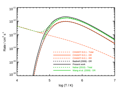
Figure 5: Total DR rate coefficients.

Dielectronic recombination (DR) from He⁺ has normally not been included in previous CRM, as for nebular astrophysics the dominant recombination rate is the RR. However, for our hot coronal conditions the DR is obviously a dominant recombination process.

We initially included in the models the level-resolved DR rate coefficients produced by NRB as part of the DR project (Badnell et al., 2003), calculated with autostructure and a few post-processing tools. These values are nearly universally used to model laboratory and astrophysical spectra, and are included in all the main atomic codes (e.g. CLOUDY, CHIANTI, ATOMDB).

However, when comparing the total rates with other published literature values, we found a significant discrepancy, of about a factor of two. On the other hand, the results of Wang et al. (1999) and Nahar (2010) were relatively close, as was the most accurate calculation (according to A. Burgess), carried out by J.Dubau during his PhD. Unfortunately, none of the published calculations were usable for our models. For example, Nahar (2010) only provided tabulated rates for a few levels.

The reasons for the lower DR rates obtained by Badnell et al. (2003) for this ion turned out to be related to orbital orthogonalisation. K-shell problems are best described by non-orthogonal orbitals, if one is using a unique orbital basis. When the H-like sequence was originally calculated 25 years ago, autostructure always Schmidt-orthogonalized. Since then, it has been realised that it is better to follow Cowan’s method (Cowan, 1981), i.e. do not orthogonalize, but just neglect the overlaps, for orbitals that are inherently non-orthogonal. For He+, the overlaps are very large between the Rydberg/Continuum s,p orbitals and the 1s, 2s, 2p. This affects the Auger rates, but the DR cross section is not sensitive to them until n-values larger those measured by the original experiment and which was used to benchmark the AS calculation.

The effect drops-off very quickly along the isoelectronic sequence with Z since the overlaps rapidly diminish then. By C⁵⁺, the increase in the total is barely 10%. We (NRB) have redone the calculations for these ions. The revised values for the H-like sequence can be found on our UK APAP web site.

Figure 5 provides a comparison between total DR rate coefficients. At 1 MK, the rate coefficient as calculated by Dubau (1973) is 9.3$\times 10^{-13}$cm³/s, that calculated by Nahar (2010) is 8.94$\times 10^{-13}$cm³/s, while the earlier DR project value was 4.56$\times 10^{-13}$cm³/s. The revised value with the Intermediate Coupling (IC) calculations is 1.0$\times 10^{-12}$cm³/s, i.e. about a factor of two higher. This resulted in a direct increase in the emissivities of the neutral He lines, as DR is the main recombination process in the corona.

Finally, for our models we needed to map the $LS$-resolved and $n$-resolved rates (by interpolation in $n$) to the level ordering in each model. It turns out that at most about half of the total DR goes to the $LS$-resolved levels but to include all the DR (within a few percent at most) we needed to include $n$-resolved levels up to $n=300$ (the values are usually calculated up to $n=999$).

2.13 Photo-excitation (PE) for He and He⁺

To include photo-excitation (PE) in the model for He and He⁺, we have used a modified version of the CHIANTI codes: once the matrices with the A-values are built, the photo-excitation and de-excitation rates are included for all the possible transitions (calculating the wavelengths from the differences in energies), using a dilution factor and radiation function. We experimented with both a black-body of a temperature between 5800 and 6100 K, and observed spectra.

For the incident radiation field we have assumed as a baseline the 1 Å-resolution quiet Sun reference irradiance spectrum compiled by Woods et al. (2009), because it covers a wide spectral range, from the X-rays to 2.5 microns, and is relatively well calibrated. We have converted the irradiances to radiances assuming uniform distribution on disk. This is a relatively good assumption for the quiet Sun. It neglects the limb-brightening effects but as we are not interested here to polarization, they can be ignored. The radiances obtained in this way compare well with on-disk radiances measured by e.g. the SoHO spectrometers. Clearly, at UV/EUV wavelengths the spectrum can differ significantly from that of the quiet Sun. This will be explored in a follow-up paper.

As the local ions have significant thermal velocities in the corona, the radiation they experience does not have the fine structure (Fraunhofer lines in absorption) of the solar spectrum emitted from the disk. We have therefore applied a smoothing to the solar spectrum, and extended it with that of a black body at 6,100 K for the infrared wavelengths, between 2.5 and 50 microns.

For the important transitions, we have used the following disk radiances: for the 10830 Å line 902681 ergs cm^-2 s^-1 sr^-1, obtained from SORCE SIM measurements; for the 584 Å line 500.5 ergs cm^-2 s^-1 sr^-1, obtained from SoHO CDS measurements of the quiet Sun, while for the He⁺ 303.8 Å line we have used the quiet Sun value of 4800 ergs cm^-2 s^-1 sr^-1 (see Del Zanna & Andretta, 2015, and references therein). We have analysed the SORCE SIM data and have found that solar variability does not significantly affect the radiance at 10830 Å. On the other hand, Andretta & Del Zanna (2014); Del Zanna & Andretta (2015) have shown that radiances and irradiances of the EUV lines can vary substantially with the solar cycle (the irradiances of the He and He+ lines vary by about a factor of two). Therefore, further modeling will be needed to study the coronal emission when the Sun is active.

Finally, we note that the photoexcitation of the strong EUV/UV lines depends significantly on the local coronal Doppler velocity, as comparatively little continuum emission is present at those wavelengths. Therefore, there is the diagnostic potential for measuring outflow velocity via Doppler dimming/brightening effects in the He II 304 Å line, as discussed in a follow-up paper. This is the same principle that has been used extensively in the literature to measure outflows using the H I Ly-$\alpha$, following Kohl & Withbroe (1982); Noci et al. (1987).

2.14 Photo-ionization (PI) for He and He⁺

Photo-ionization (PI) is an important process which is not currently included in CHIANTI. The fits to the photoionisation cross-sections provided by Verner et al. (1996) are widely used in the literature in most photoionisation codes (e.g. CLOUDY), however they are only the total cross-sections from the ground states. They were obtained by fitting the Opacity Project (OP, see Seaton et al. 1994; Seaton 2005) cross-sections, by removing the resonances and adjusting the thresholds to observation. Clearly, for our models, photoionisation from excited states is important. As PI is the inverse process of RR, photoionisation cross-sections from the lower levels have been calculated with autostructure (Badnell, 2006). We have verified that these three sets of cross-sections agree for the ground state.

For the PI from higher levels we have used the semi-classical Kramers hydrogenic formula in the form:

$$\sigma(\lambda;n_{i})=8.68896\,10^{-37}\>E_{i}^{2}\>n_{i}^{-2}\>\lambda^{3}\>,$$

where the cross-section $\sigma$ is in cm², $\lambda$ is the ionizing photon wavelength in Å, and $E_{i}$ are $n_{i}$ are respectively the ionization threshold and the principal quantum number of level $i$. For levels with $n\leq 5$ we have also applied the Gaunt factors from Karzas & Latter (1961). In the application of the above formula to He⁰ we have used the observed ionization energies, verifying that the results reasonably match the detailed OP calculations, when available.

We have also experimented in using the OP values, whenever available, by adjusting the thresholds. The end results do not change significantly, but we opted for the semi-classical cross-sections as the effects due to the incorrect location and low resolution of the resonances in the OP data are difficult to quantify.

For the incident radiation field we have assumed the same solar spectrum used for PE.

3 Benchmark at low-temperature

Table 1: Emissivities (10^-26 erg cm³ s^-1 ) of the strongest He lines, for $T{\rm e}$=20,000 K and $N_{\rm e}$=10⁶ cm^-3.

$\lambda$ (Å)	levels	P05 (B)	P12 (B)	F (A)	F (B)
584	S 2p-1s			162
2945	T 5p-2s	2.96	2.22	2.16	2.16
3188	T 4p-2s	6.51	5.09	5.0	5.0
3889	T 3p-2s	18.3	15.0	14.9	14.9
3965	S 4p-2s	1.54	1.21	0.034	0.99
4026	T 5d-2p	3.18	2.01	1.94	1.94
4388	S 5d-2p	0.83	0.57	0.42	0.44
4471	T 4d-2p	6.80	4.71	4.40	4.40
4713	T 4s-2p	0.92	1.05	1.06	1.06
4922	S 4d-2p	1.80	1.31	0.90	0.93
5016	S 3p-2s	4.04	3.17	0.06	2.64
5876	T 3d-2p	20.2	18.3	15.7	15.7
6678	S 3d-2p	5.22	4.88	2.64	2.75
7065	T 3s-2p	7.17	7.62	7.65	7.67
7281	S 3s-2p	1.36	1.30	0.88	1.18
10830	T 2p-2s	255	215	213	214
18685	T 4f-3d	2.37	0.85	1.15	1.15
20587	S 2p-2s	-	5.98	5.1$\times$10-3	5.0

As previously mentioned, we found it useful to benchmark our largest $n=40$ model at low temperatures against previous sophisticated CRM. We have chosen for the benchmark $T$=20,000 K and an electron density $N$=10⁶ cm^-3, allowed by our $n$=40 model. The most complex CRM for neutral He were developed for nebular astrophysics, see for example Brocklehurst (1972); Smits (1991, 1996); Benjamin et al. (1999); Porter et al. (2005, 2012) for neutral He and Hummer & Storey (1987) for ionised He. The basic atomic rates have changed over the years, and each model was different. The approach in the earlier studies was often to solve the statistical balance equations in terms of departure coefficients $b$ from Saha-Boltzmann level populations. The calculations usually considered only $n$-resolved levels to start with, then the $b_{nl}$ for the terms (in LS coupling) were calculated, assuming that higher levels were statistically redistributed in $l$. Matrix condensation techniques were often employed to reduce the number of levels. Collisional ionization from the metastable level of He (or higher ones) was usually not included. Photo-excitation and photo-ionization from anything other than the ground state was also generally not included.

The latest two CRM on He are from Porter et al. (2005, 2012), and are based on codes available within the CLOUDY photoionisation code (Ferland et al., 2017), although we note that several improvements on atomic rates (especially on the l-changing collisions) have been (and are still) ongoing in CLOUDY. We have chosen these two models not just because they are more recent, but especially because they used the same CE as we do in our model, from Bray et al. (2000). In fact, some differences in the line emissivities are known to be caused by the use of different CE rates.

As the main published results are line emissivities of the pure He recombination spectrum, we had to apply a few modifications to our coronal model. The first one is to remove He⁺⁺ and apply a black-body photo-ionizing spectrum with a dilution of 1.74 $\times$ 10^-11 and $T$=100,000 K to obtain well over 99% of the population in He⁺, and simulate the effects of a hot star driving a He recombination spectrum. The second one is to remove the DR (as normally not included in previous models, being negligible at low temperatures), and use improved RR rates obtained from the state-of-the-art photo-ionization cross-sections by Hummer & Storey (1998). We used $LS$-resolved RR rates up to $n$=40, then $n$-resolved rates up to $n$=99.

The emissivities are usually presented in the literature for case A and case B. Case A is simply assuming an optically thin plasma. Most literature values are in case B, which is an approximation to model the real plasma emission when the strongest singlet lines, decaying to the ground state, are re-absorbed. To obtain the case B, we have set to zero the RR to the ground state and all the A-values of the singlet (above $n$=2) decays to the ground state.

The emissivities are

$$E=\frac{4\,\pi\,j}{N_{\rm e}\,N(He^{+})}=\frac{h\,\nu_{ji}\,N_{j}\,A_{ji}\,N(He)}{N_{\rm e}\,N(He^{+})}\quad{\rm erg\,cm}^{3}\,{\rm s}^{-1}$$ (1)

where the first definition is how the emissivities are usually indicated in the literature, and the second one is how we calculated them: $N_{j}$ is the population of the upper level $j$, relative to the total population of He, N(He), i.e. He⁰ and He⁺; $A_{ji}$ is the radiative transition rate, and $h\,\nu_{ji}$ is the energy of the photon.

The resulting emissivities for all the strongest He lines in the visible/near infrared are shown in Table 1. There is generally a good agreement with the latest published results by Porter et al. (2012), which indicates that the present model is correct. However, significant differences are present with Porter et al. (2005), and also with earlier studies (not shown in the Table). We note that we did not expect to see such differences between the various models, as one would expect accuracy of a few percent, but defer to a follow-up paper a full discussion on the reasons for such discrepancies.

We experimented with different rates for collisional excitation to the higher levels, as well as different rates between the higher levels (l-changing collisions), but our results were unchanged. We also noticed that collisional ionization does not have a large effect at these low densities. The main populating processes for the upper levels of the lines shown in the Table are the RR from He⁺ and collisional excitation from the metastable states.

4 Results for coronal plasma

4.1 He I vs. Fe XIII

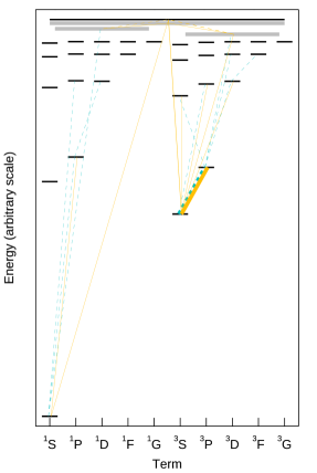
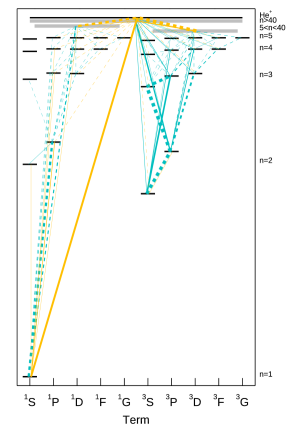
Figure 6: The main transition rates for He I. The strongest net brackets, $n_{i}P_{ij}-n_{j}P_{ji}$, are shown: orange lines represent collisional net brackets (including radiative recombinations), azure represent net radiative brackets (photoexcitations/ionisations, spontaneous/stimulated transitions). Upward and downward net rates are represented by dashed and solid lines, respectively. Only net brackets whose absolute value is greater than 1/100^th of the largest net bracket are shown. Left and right panels show net rates in the case of zero and non-zero external radiation field, respectively, computed at 1.05  $\rm R_{\odot}$. In both cases, the electron density and temperature are $\log n_{\mathrm{e}}=8$ and $\log T=6$, respectively.

Figure 7: Emissivities of the 10830 Å line obtained with the four collisional-radiative models, without photo-excitation (PE) and photo-ionization (PI) (dashed lines), with PE (dot-dashed lines) and with both PE and PI (full lines). The emissivities calculated with the CHIANTI He model are also shown, as well as those of the Fe XIII NIR line (with and without PE - PI is not affecting this ion). The top plot shows the values at a density for the solar quiet corona near the limb, and with PE/PI at 1.05  $\rm R_{\odot}$. The lower plot shows the values at a lower density of the outer corona, and with PE/PI at 1.5 $\rm R_{\odot}$.

The He I 10830 Å line is very close in wavelength to the two well-known forbidden lines from Fe XIII, the 3s² 3p^{2 3}P₁-3s² 3p^{2 3}P₂ at 10798 Å and the 3s² 3p^{2 3}P₀-3s² 3p^{2 3}P₁ at 10747 Å (all wavelengths in air). These three lines are a primary objective for the coronal DKIST observations.

The eclipse observations by Kuhn et al. (1996) of a quiescent streamer clearly showed that close to the solar limb the three lines have comparable intensities. With increasing radial distance from the Sun, the Fe XIII 10798 Å decreases its intensity significantly, while the two other lines show a much slower decrease. From the Fe XIII modelling we know that the 10798 Å is relatively insensitive to PE, while the 10747 Å becomes strongly photo-excited with decreasing electron densities.

As the observed radiances are the product of the local emissivities and the local densities integrated along the line of sight (alos), comparisons with observations are strongly model-dependent. We defer such modelling to a future paper.

For the present paper, we have chosen to present a comparison of the local emissivities of the He lines with that of the Fe XIII 10798 Å line for two typical distances from the Sun which are relevant for DKIST: 1.05 and 1.5  $\rm R_{\odot}$ from Sun centre. At these distances, our estimated local densities in quiescent streamers are approximately 10⁸ and 10⁷ cm^-3 respectively.

On a side (but important) note, we would like to point out that the emissivities of the Fe XIII forbidden lines can be used as a reference as the atomic model, based on the latest calculations by Del Zanna & Storey (2012) and available since CHIANTI version 8 (Del Zanna et al., 2015), is relatively accurate. In fact, their intensities have not changed significantly, compared to models based on the earlier (smaller) calculations by Storey & Zeippen (2010). These lines are strongly affected by cascading effects from higher levels. Hence, proper atomic modelling typically requires a few hundreds of levels and very accurate rates. This is discussed in Del Zanna & Mason (2018). PE effects are significant, but can be calculated accurately. PI effects are negligible, unless there is a solar flare.

By contrast, PI effects, as discussed further below, can be important in determining the He I level populations and, in particular, the 10830 Å line emissivity.

More generally, useful insight into the main processes determining the He I level populations can be obtained by inspecting the most important net rate brackets between the levels, $n_{i}P_{ij}-n_{j}P_{ji}$, where $P_{ij}$ and $P_{ji}$ are either the radiative or collisional rates between levels $i$ and $j$. As an example, Figure 6 displays the main net radiative and collisional brackets at $n_{\mathrm{e}}=10^{8}$ cm^-3 and $T=10^{6}$ K, at 1.05  $\rm R_{\odot}$. For clarity of display, only rates between levels with $n\leq 5$ are shown in detail. Levels with $5<n\leq 40$ are grouped in two “average levels” (shown as gray blocks), one for singlets and another triplets, while levels with $n>40$ are shown as a single average level.

To highlight the role of PE and PI, the left-hand panel shows the main terms in the statistical equilibrium equations in the purely collisional case. In this case, the excited levels are populated mainly by radiative cascades from He⁺ following collisional ionization from the ground level.

As discussed more quantitatively below, when PE and PI are taken into account (right-hand panel), the populations of the triplets become dominated by radiative processes due to the high level of illumination by optical radiation (UV, visible and IR) from the solar disk. Thus, the metastable level $1s2s^{3}S$ becomes crucial in determining the relative populations of the triplet levels. In particular, the relative populations of levels connected via permitted transitions to level $1s2s^{3}S$ are “locked” to values dictated by the PE radiation field, nearly independently on temperature and density.

The emissivities for both He I and Fe XIII lines are calculated with a grid of electron temperatures. As a guideline, we expect the local temperature close to the Sun to be around 1 MK, increasing with height to a value around 1.4 MK. Such a value was obtained from SoHO UVCS 1999 observations of two coronal lines in the 1.4–3  $\rm R_{\odot}$ range (Del Zanna et al., 2018). A similar temperature was also obtained from NIR observations of forbidden lines by AIR-Spec during the 2017 eclipse (Madsen et al., 2019).

We note that, as the distance, density, and temperature are fixed, and as the PE and PI radiances from the solar disk are well known, the results shown here basically only depend on the atomic rates included in the models. For Fe XIII, we adopted the version 8 CHIANTI model and ion charge states. We adopted photospheric abundances, as there is now converging evidence that they better represent the quiescent solar corona (see the recent review in Del Zanna & Mason, 2018). However, as already known for other elements, there seems to be a significant spatial variability in the coronal He abundance, as discussed in Moses & et al. (2020) and references therein. Therefore, the present emissivities should be taken as indicative.

In order to discuss in more detail how the different processes affect the line emissivities, we present first in Figure 7 (top) the emissivities of the He 10830 Å line, obtained with the four different CRM: $n=10,20,30,40$ for a density of 10⁸ cm^-3 (the lower dashed lines). We then show with the dot-dashed lines the same results obtained with PE, and with full lines those with PE and PI. Considering first the case without PE and PI, it is clear that the different models show similar results. It is interesting to note that, despite the numerous differences in the rates, the emissivities calculated with the present CHIANTI model are not far from our calculated ones. The same holds for the other He lines as shown below. It is also clear that the intensity of the He 10830 Å line is about two orders of magnitude lower than that of the Fe XIII 10798 Å line at 1 MK.

At 1 MK, the population of the 2p ³P, upper level of the He 10830 Å transition, is due by 85% to collisional excitation from the metastable 2s ³S, the rest from cascading mostly from higher ³S and ³D. In turn, they are populated by further cascading, DR from He⁺, and collisional excitation from the metastable 2s ³S. The relative population (over the whole He) of the 2s ³S level is 9.1 $\times$ 10^-11, that of the ground state is 3.9 $\times$ 10^-10 and that of the 2p ³P is 1.1 $\times$ 10^-15. The emissivity of the He 10830 Å line is directly related to the total DR rate to the triplets from the ground state of He⁺, hence to the population of this state. In turn, the ground state of He⁺ is relatively well constrained by the CI from (and DR to) He, plus CI (and RR from) to He⁺⁺.

The results obtained when including PE (dot-dashed lines) are completely different. The first main result to note is the large increase in the emissivity of the He 10830 Å line, by nearly three orders of magnitude. The second result is the fact that the $n=10,20$ models are insufficient to properly estimate the He 10830 Å line. The $n=30$ model appears sufficient, as the more complex $n=40$ model basically provides the same values.

The reason for this emissivity increase is the cumulative effect of PE over many transitions, with consequent cascading to increase by orders of magnitude the population of the ³P, the upper level of the He 10830 Å line. When PE is switched on, all the levels that are connected to the metastable 2s ³S via transitions in the visible and near infrared are photo-pumped by the large number of photons radiating from the disk. The population of the metastable drops to 2.9 $\times$ 10^-12 (that of the ground state is 4.1 $\times$ 10^-10) and the upper level 2p ³P is now populated by 93% by the 10830 Å photons, with a relative population of 3.3 $\times$ 10^-13. The remaining population is mainly via cascading from the 3d ³D (5877 Å), and 3s ³S (7067 AA), so also these levels are photo-pumped. With PE, the 2p ³P also increases the populations of the 4s ³S (4714 Å), 4d ³D (4472 Å), 5s ³S (4121 Å), and 5d ³D (4027 Å), so in practice all the triplets have increased populations (see again Fig. 6.

Figure 8: b-factors for the solar corona near the limb, without (above), with (middle) photo-excitation (PE), and with both PE and photo-ionisation (PI), below, obtained with the larger $n=40$ model.

One synthetic way to show this effect is to plot the b-factors, i.e. the deviations from the Saha-Boltzmann population (relative to the ground state of He⁺), as shown in Figure 8. The top plot shows the b-factors without PE. Note that the relative populations of the singlets and triplets converge to the values of the $n$-levels. At sufficiently high principal quantum numbers, the $n$-levels converge to a Saha-Boltzmann population. The middle plot shows the b-factors with PE included, where it is clear that all the triplet levels have increased populations.

We also noted that some differences are obtained when the observed spectrum is used instead of a black-body. Long-wavelength photons in the IR above 2.5 microns also play a role, while those below 2000 Å are insignificant. For more accurate modelling, it would be useful to have observations of the infrared continuum. Solar variability should not have a large effect, as observations of the visible/NIR spectrum show very little changes with the solar cycle.

The addition of PI dramatically affects the population of the metastable He triplet level, which drops to 5.9 $\times$ 10^-13 (that of the ground state only has a small decrease to 3.8 $\times$ 10^-10). As a consequence, the upper level 2p ³P of the 10830 Å  has a much lower relative population of 6.7 $\times$ 10^-14, and the emissivity of the line therefore decreases accordingly. Still, the emissivity of the He line is comparable to that of the reference Fe XIII line, around 1 MK. The decrease in the population of the triplets is clear in the b-factors, shown in Figure 8 (bottom).

If only PI and not PE was present, the main effect would be photoionisation of the two 2s ^1,3S levels. However, when both PE and PI are included in the model, photoionisation of the lower excited levels has a cumulative effect lowering the 2p ³P population by a factor of about two. The main reason this PI is so effective is the fact that the thresholds are close to the peak solar disk emission in the visible. For example, the PI edge of the 2s ³S is around 2600 Å(in the MUV), where a significant amount of photons are emitted by the solar surface (still significantly less than assuming a black body).

The solar composite spectrum of Woods et al. (2009) has for the MUV wavelengths data from the SORCE Solar Stellar Irradiance Comparison Experiment (SOLSTICE) MUV channel. Woods et al. (2009) noted a difference of about 10% compared to earlier ATLAS-3 measurements. This is larger than the quoted uncertainties in the measurements. Regarding solar variability, it is well known that variations around these wavelengths are not as large as in the FUV/EUV. For example, Rottman (2000) shows that cycle variations at wavelengths shortward of 2600 Å are at most a few percent. Variations and uncertainties in the visible are even less.

The emissivities of the 10830 Å line at 1.5  $\rm R_{\odot}$, calculated without PE, are shown in Figure 7 (below). The results are somewhat similar to the previous ones near the limb. As one would expect, the emissivities obtained when including PE are even more pronounced, as in this case the density is much lower, 10⁷ cm^-3. A lower local density increases the PE effects relative to collisional processes. It should be noted that this time even the $n=30$ model did not appear to have reached full convergence, as the much larger $n=40$ model provides slightly higher emissivities. The final case with PE and PI is also similar to the previous case, although the emissivity of the 10830 Å line is now higher. There is clearly a strong temperature sensitivity: at 1 MK the 10830 Å line emits a lot more photons than the Fe XIII 10798 Å line, but at 1.3 MK the He line should be much weaker by over an order of magnitude.

4.2 He I D₃ and 584 Å lines

Figure 9: Emissivities of the He I D₃ line obtained with the four collisional-radiative models, without photo-excitation (PE) and photo-ionization (PI) (dashed lines), with PE (dot-dashed lines) and with both PE and PI (full lines). The emissivities calculated with the CHIANTI He model are also shown, as well as those of the Fe XIII NIR line, with and without PE (PI is not affecting this ion). The top plot shows the values at a density for the solar quiet corona near the limb, and with PE/PI at 1.05  $\rm R_{\odot}$. The lower plot shows the values at a lower density of the outer corona, and with PE/PI at 1.5 $\rm R_{\odot}$. Note the different scale compared to the 10830 Å plot.

Figure 9 shows the emissivities of the D₃ line, presented in the same way as those of the 10830 Å transition (but on a different scale). Being a triplet transition, this line is affected by the same processes as the 10830 Å one, and the overall results are very similar. The $n$=30 model shows convergence, and the same patterns when PE and PI are present. The emissivity of the D₃ line, however, even at 1 MK is predicted to be over one order of magnitude weaker than the Fe XIII line, hence it might not be visible by ASPIICS outside of prominences.

Figure 10: Emissivities of the He 584 Å resonance line obtained with the four collisional-radiative models, displayed as in Figure 9 for the solar quiet corona near the limb, and with PE/PI at 1.05  $\rm R_{\odot}$.

Figure 10 shows the results for the resonance line at 584 Å, the decay from the ¹P directly to the ground state, for the solar quiet corona near the limb, and with PE/PI at 1.05  $\rm R_{\odot}$. As there are comparatively very few photo-exciting photons originating from the disk, PE hardly has any effect on this line (and on any other lines of the principal series). We therefore predict that this line should be about three orders of magnitude weaker than the Fe XIII NIR line, i.e. practically invisible. Our findings are consistent with the lack of observations of that line by SoHO UVCS in the near-Sun corona that could be unambiguously be attributed to coronal plasma (see Sec. 1).

4.3 Ionised helium

Figure 11: Emissivities of the main He⁺ resonance line at 304 Å for the solar corona near the limb at 1.05  $\rm R_{\odot}$ (top) and at 1.5 $\rm R_{\odot}$ without and with photo-excitation (PE) and photo-ionisation (PI), obtained with the largest $n=40$ collisional-radiative model. The emissivity of the Fe XIII NIR line with (and without) PE is shown with a full (dashed) line for comparison. Note the different scale compared to the the 10830 Å plot.

The modelled emissivities of the main He⁺ resonance line are shown in Figure 11 in the same way as those of the 10830 Å transition (but on a different scale). This line is strongly affected by photo-excitation (PE), especially at low electron densities. Therefore, direct measurements of the variable disk radiation will be needed for detailed models. On the other hand, its emissivity is rather insensitive to the model used or to photo-ionisation (PI) for coronal temperatures. The emissivities are close to those obtained with the CHIANTI model (modified to input the same resonant PE), mainly because in both cases the same ionization and recombination rates to He⁺⁺have been used, and because the same He⁺ ion model is adopted.

5 Conclusions

As a result of a careful assessment of all the rates and the effects of photo-excitation and photo-ionisation on progressively more extensive collisional-radiative models, we are able to recommend a model to be used to study the helium emission in the solar corona. The key issue for the neutral He emission is that a fully $LS$-resolved set of states up to $n=40$, and $n$-resolved states up to $n=300$ are required. The complexity of this model is similar to the most extensive models developed to study He for photo-ionised gas in nebulae, but in very different conditions, i.e. much lower temperatures and densities than in the coronal case. The revised dielectronic recombination rates presented here resulted in a significant (factor of two) increase in the abundance of neutral He.

Regarding He⁺, we confirm that the resonance 304 Å line is a strong coronal line, mainly because at coronal temperatures He⁺ has a significant abundance. This line also has a strong resonantly scattered component which increases its intensity. Therefore, solar variability plays an important role, as the disk radiation is variable. As the intensity of this line is directly related to the population of the ground state of He⁺, which in turn affects the population of the He levels by DR, an ideal observational benchmark of the present model would include simultaneous observations of the He and He⁺ lines. Indirect measurements will be possible with a combination of Solar Orbiter and DKIST observations.

Regarding neutral He, as described in the introduction, several possible explanations have been put forward to explain the apparently anomalous high intensity of the 10830 Å line in the outer corona. We note that in general, various mechanisms could be at play. The purpose of the present paper was not to discuss them, but provide a key missing element: a prediction of the coronal emission of the main He I lines, in the light of the new polarimetric measurements by DKIST and Proba-3 which in principle will provide a novel way to measure the magnetic field in the low corona.

The present models indicate that a significant coronal emission of the 10830 Å line should be present close to the solar limb, for an electron temperature of 1 MK. In this case, the intensity of this line should be comparable to that of the well-studied Fe XIII 10798 Å line, one of the strongest forbidden lines in the solar corona (Del Zanna & DeLuca, 2018). This appears in line with observations and is mainly due to a complex system of photo-excitation (PE) and photo-ionisation (PI) due to the disk radiation, with subsequent cascading (and recombination followed by cascading) to over-populate the upper level of this transition. The PE and PI effects are sensitive to the solar spectrum. We have briefly mentioned where accurate measurements would be useful. We also expect that some minor solar variability effects would be present.

However, in the outer corona, the emissivity of the 10830 Å line should decrease significantly, with respect to the Fe XIII 10798 Å line. The actual observed emission would mainly be the result of a fine balance between the distributions of electron densities and temperatures along the line of sight. Independent measurements of the density and its fine structure with e.g. a combination of the Fe XIII NIR and EUV lines would be needed for a proper modelling of the He I lines, as well as estimates of the electron temperature, which is harder to measure. Finally, the coronal abundance variability needs to be taken into account.

The He I D₃ line is also affected strongly by PE and PI, although this feature is much weaker and might not be observable. On the other hand, the EUV resonance 584 Å  line is not pumped by PE, and should be unobservable. Any observations of the 584 Å  line in the outer corona would be important, as they would indicate that other processes augment the He emission, as for example the presence of dust or cool gas from e.g. erupting prominences, as proposed in the literature.

We plan to apply the present models to provide more detailed predictions of the expected helium emission in the corona, as will be observed by several new facilities, by taking into account the key input parameters and their variability. We also plan to apply them to revisit the modelling of the He lines in the transition region, i.e. at lower temperature and higher density conditions.

As the basic rates and models are very general, we also plan to extend them to predict the recombination spectrum of He for nebular conditions. The comparison with literature values at the lowest density achievable by the largest model has clearly indicated that improvements on previous studies can be made.

References

- Alder et al. (1956) Alder, K., Bohr, A., Huus, T., Mottelson, B., & Winther, A. 1956, Reviews of Modern Physics, 28, 432, doi: 10.1103/RevModPhys.28.432
- Andretta & Del Zanna (2014) Andretta, V., & Del Zanna, G. 2014, A&A, 563, A26, doi: 10.1051/0004-6361/201322841
- Andretta et al. (2003) Andretta, V., Del Zanna, G., & Jordan, S. D. 2003, A&A, 400, 737, doi: 10.1051/0004-6361:20021893
- Andretta et al. (2012) Andretta, V., Telloni, D., & Del Zanna, G. 2012, Sol. Phys., 279, 53, doi: 10.1007/s11207-012-9974-z
- Antonucci et al. (2019) Antonucci, E., Romoli, M., Andretta, V., et al. 2019, arXiv e-prints, arXiv:1911.08462. https://arxiv.org/abs/1911.08462
- Badnell (2006) Badnell, N. R. 2006, ApJS, 167, 334, doi: 10.1086/508465
- Badnell (2011) Badnell, N. R. 2011, Computer Physics Communications, 182, 1528, doi: 10.1016/j.cpc.2011.03.023
- Badnell et al. (2003) Badnell, N. R., O’Mullane, M. G., Summers, H. P., et al. 2003, A&A, 406, 1151, doi: 10.1051/0004-6361:20030816
- Ballance et al. (2006) Ballance, C. P., Griffin, D. C., Loch, S. D., Boivin, R. F., & Pindzola, M. S. 2006, Phys. Rev. A, 74, 012719, doi: 10.1103/PhysRevA.74.012719
- Bates & Damgaard (1949) Bates, D. R., & Damgaard, A. 1949, Philosophical Transactions of the Royal Society of London Series A, 242, 101, doi: 10.1098/rsta.1949.0006
- Benjamin et al. (1999) Benjamin, R. A., Skillman, E. D., & Smits, D. P. 1999, ApJ, 514, 307, doi: 10.1086/306923
- Bray et al. (2000) Bray, I., Burgess, A., Fursa, D. V., & Tully, J. A. 2000, A&AS, 146, 481, doi: 10.1051/aas:2000277
- Breeveld et al. (1988) Breeveld, E. R., Culhane, J. L., Norman, K., et al. 1988, Astrophysical Letters and Communications, 27, 155
- Brocklehurst (1972) Brocklehurst, M. 1972, MNRAS, 157, 211, doi: 10.1093/mnras/157.2.211
- Burgess & Summers (1969) Burgess, A., & Summers, H. P. 1969, ApJ, 157, 1007, doi: 10.1086/150131
- Burgess & Summers (1976) —. 1976, MNRAS, 174, 345, doi: 10.1093/mnras/174.2.345
- Burgess & Tully (1978) Burgess, A., & Tully, J. A. 1978, Journal of Physics B Atomic Molecular Physics, 11, 4271, doi: 10.1088/0022-3700/11/24/019
- Burgess & Tully (1992) Burgess, A., & Tully, J. A. 1992, A&A, 254, 436
- Cowan (1981) Cowan, R. D. 1981, The theory of atomic structure and spectra (Los Alamos Series in Basic and Applied Sciences), 361–365
- Dall et al. (2008) Dall, R. G., Baldwin, K. G. H., Byron, L. J., & Truscott, A. G. 2008, Phys. Rev. Lett., 100, 023001, doi: 10.1103/PhysRevLett.100.023001
- Del Zanna & Andretta (2015) Del Zanna, G., & Andretta, V. 2015, A&A, 584, A29, doi: 10.1051/0004-6361/201526804
- Del Zanna & DeLuca (2018) Del Zanna, G., & DeLuca, E. E. 2018, ApJ, 852, 52, doi: 10.3847/1538-4357/aa9edf
- Del Zanna et al. (2015) Del Zanna, G., Dere, K. P., Young, P. R., Landi, E., & Mason, H. E. 2015, A&A, 582, A56, doi: 10.1051/0004-6361/201526827
- Del Zanna & Mason (2018) Del Zanna, G., & Mason, H. E. 2018, Living Reviews in Solar Physics, 15
- Del Zanna et al. (2018) Del Zanna, G., Raymond, J., Andretta, V., Telloni, D., & Golub, L. 2018, ArXiv e-prints. https://arxiv.org/abs/1808.07951
- Del Zanna & Storey (2012) Del Zanna, G., & Storey, P. J. 2012, A&A, 543, A144, doi: 10.1051/0004-6361/201219193
- Delaboudinière (1999) Delaboudinière, J. P. 1999, Sol. Phys., 188, 259, doi: 10.1023/A:1005268807716
- Dere (2007) Dere, K. P. 2007, A&A, 466, 771, doi: 10.1051/0004-6361:20066728
- Dere et al. (2019) Dere, K. P., Del Zanna, G., Young, P. R., Landi, E., & Sutherland, R. S. 2019, ApJS, 241, 22, doi: 10.3847/1538-4365/ab05cf
- Ding & Habbal (2017) Ding, A., & Habbal, S. R. 2017, ApJ, 842, L7, doi: 10.3847/2041-8213/aa7460
- Drake (1986) Drake, G. W. F. 1986, Phys. Rev. A, 34, 2871, doi: 10.1103/PhysRevA.34.2871
- Drake (2006) Drake, G. W. F. 2006, Springer Handbook of Atomic, Molecular, and Optical Physics, doi: 10.1007/978-0-387-26308-3
- Drake & Morton (2007) Drake, G. W. F., & Morton, D. C. 2007, ApJS, 170, 251, doi: 10.1086/512239
- Dubau (1973) Dubau, J. 1973, PhD thesis, Univ. College London, UK
- Dufresne & Del Zanna (2019) Dufresne, R. P., & Del Zanna, G. 2019, arXiv e-prints, arXiv:1901.08992. https://arxiv.org/abs/1901.08992
- Fehlmann et al. (2016) Fehlmann, A., Giebink, C., Kuhn, J. R., et al. 2016, in Proc. SPIE, Vol. 9908, Ground-based and Airborne Instrumentation for Astronomy VI, 99084D, doi: 10.1117/12.2232218
- Ferland et al. (2017) Ferland, G. J., Chatzikos, M., Guzmán, F., et al. 2017, Rev. Mexicana Astron. Astrofis., 53, 385. https://arxiv.org/abs/1705.10877
- Fursa & Bray (2003) Fursa, D. V., & Bray, I. 2003, Journal of Physics B Atomic Molecular Physics, 36, 1663, doi: 10.1088/0953-4075/36/8/317
- Gabriel (1971) Gabriel, A. H. 1971, Sol. Phys., 21, 392, doi: 10.1007/BF00154290
- Gabriel et al. (1995) Gabriel, A. H., Culhane, J. L., Patchett, B. E., et al. 1995, Advances in Space Research, 15, 63, doi: 10.1016/0273-1177(94)00020-2
- Génévriez et al. (2017) Génévriez, M., Jureta, J. J., Defrance, P., & Urbain, X. 2017, Phys. Rev. A, 96, 010701, doi: 10.1103/PhysRevA.96.010701
- Giordano et al. (2013) Giordano, S., Ciaravella, A., Raymond, J. C., Ko, Y. K., & Suleiman, R. 2013, Journal of Geophysical Research (Space Physics), 118, 967, doi: 10.1002/jgra.50166
- Goldberg (1935) Goldberg, L. 1935, ApJ, 82, 1, doi: 10.1086/143654
- Golding et al. (2017) Golding, T. P., Leenaarts, J., & Carlsson, M. 2017, A&A, 597, A102, doi: 10.1051/0004-6361/201629462
- Guzmán et al. (2017) Guzmán, F., Badnell, N. R., Williams, R. J. R., et al. 2017, MNRAS, 464, 312, doi: 10.1093/mnras/stw2304
- Guzmán et al. (2019) Guzmán, F., Chatzikos, M., van Hoof, P. A. M., et al. 2019, MNRAS, 486, 1003, doi: 10.1093/mnras/stz857
- Havener et al. (2005) Havener, C. C., Rejoub, R., Krstić, P. S., & Smith, A. C. H. 2005, Phys. Rev. A, 71, 042707, doi: 10.1103/PhysRevA.71.042707
- Hummer & Storey (1987) Hummer, D. G., & Storey, P. J. 1987, MNRAS, 224, 801, doi: 10.1093/mnras/224.3.801
- Hummer & Storey (1998) —. 1998, MNRAS, 297, 1073, doi: 10.1046/j.1365-8711.1998.2970041073.x
- Judge et al. (2019) Judge, P., Berkey, B., Boll, A., et al. 2019, Sol. Phys., 294, 166, doi: 10.1007/s11207-019-1550-3
- Karzas & Latter (1961) Karzas, W. J., & Latter, R. 1961, ApJS, 6, 167, doi: 10.1086/190063
- Kingdon & Ferland (1996) Kingdon, J. B., & Ferland, G. J. 1996, ApJS, 106, 205, doi: 10.1086/192335
- Kohl & Withbroe (1982) Kohl, J. L., & Withbroe, G. L. 1982, ApJ, 256, 263, doi: 10.1086/159904
- Kohl et al. (1995) Kohl, J. L., Esser, R., Gardner, L. D., et al. 1995, Sol. Phys., 162, 313, doi: 10.1007/BF00733433
- Kuhn et al. (2007) Kuhn, J. R., Arnaud, J., Jaeggli, S., Lin, H., & Moise, E. 2007, ApJ, 667, L203, doi: 10.1086/522370
- Kuhn et al. (1996) Kuhn, J. R., Penn, M. J., & Mann, I. 1996, ApJ, 456, L67, doi: 10.1086/309864
- Łach & Pachucki (2001) Łach, G., & Pachucki, K. 2001, Phys. Rev. A, 64, 042510, doi: 10.1103/PhysRevA.64.042510
- Lallement et al. (2004) Lallement, R., Raymond, J. C., Vallerga, J., et al. 2004, A&A, 426, 875, doi: 10.1051/0004-6361:20035929
- Laming & Feldman (2001) Laming, J. M., & Feldman, U. 2001, ApJ, 546, 552, doi: 10.1086/318238
- Laming & Feldman (2003) —. 2003, ApJ, 591, 1257, doi: 10.1086/375395
- Ljepojevic et al. (1984) Ljepojevic, N. N., Hutcheon, R. J., & McWhirter, R. W. P. 1984, Journal of Physics B Atomic Molecular Physics, 17, 3057, doi: 10.1088/0022-3700/17/15/019
- Ljepojevic et al. (1987) Ljepojevic, N. N., Hutcheon, R. J., & Payne, J. 1987, Computer Physics Communications, 44, 157, doi: 10.1016/0010-4655(87)90025-7
- Loreau et al. (2018) Loreau, J., Ryabchenko, S., Muñoz Burgos, J. M., & Vaeck, N. 2018, Journal of Physics B Atomic Molecular Physics, 51, 085205, doi: 10.1088/1361-6455/aab425
- Loreau et al. (2014) Loreau, J., Ryabchenko, S., & Vaeck, N. 2014, Journal of Physics B Atomic Molecular Physics, 47, 135204, doi: 10.1088/0953-4075/47/13/135204
- Madsen et al. (2019) Madsen, C. A., Samra, J. E., Del Zanna, G., & DeLuca, E. E. 2019, ApJ, 880, 102, doi: 10.3847/1538-4357/ab2b3c
- Michels et al. (2002) Michels, J. G., Raymond, J. C., Bertaux, J. L., et al. 2002, ApJ, 568, 385, doi: 10.1086/338764
- Moise et al. (2010) Moise, E., Raymond, J., & Kuhn, J. R. 2010, ApJ, 722, 1411, doi: 10.1088/0004-637X/722/2/1411
- Morabito et al. (2014) Morabito, L. K., van Harten, G., Salgado, F., et al. 2014, MNRAS, 441, 2855, doi: 10.1093/mnras/stu775
- Moses & et al. (2020) Moses, J. D., & et al. 2020, Nature, in press
- Nahar (2010) Nahar, S. N. 2010, New A, 15, 417, doi: 10.1016/j.newast.2009.11.010
- Noci et al. (1987) Noci, G., Kohl, J. L., & Withbroe, G. L. 1987, ApJ, 315, 706, doi: 10.1086/165172
- Parpia & Johnson (1982) Parpia, F. A., & Johnson, W. R. 1982, Phys. Rev. A, 26, 1142, doi: 10.1103/PhysRevA.26.1142
- Patchett et al. (1981) Patchett, B. E., Norman, K., Gabriel, A. H., & Culhane, J. L. 1981, Space Sci. Rev., 29, 431, doi: 10.1007/BF00239488
- Pengelly & Seaton (1964) Pengelly, R. M., & Seaton, M. J. 1964, MNRAS, 127, 165, doi: 10.1093/mnras/127.2.165
- Penn et al. (1994) Penn, M. J., Arnaud, J., Mickey, D. L., & Labonte, B. J. 1994, ApJ, 436, 368, doi: 10.1086/174911
- Percival & Richards (1978) Percival, I. C., & Richards, D. 1978, MNRAS, 183, 329, doi: 10.1093/mnras/183.3.329
- Porter et al. (2005) Porter, R. L., Bauman, R. P., Ferland, G. J., & MacAdam, K. B. 2005, ApJ, 622, L73, doi: 10.1086/429370
- Porter et al. (2012) Porter, R. L., Ferland, G. J., Storey, P. J., & Detisch, M. J. 2012, MNRAS, 425, L28, doi: 10.1111/j.1745-3933.2012.01300.x
- Ralchenko et al. (2008) Ralchenko, Y., Janev, R. K., Kato, T., et al. 2008, Atomic Data and Nuclear Data Tables, 94, 603, doi: 10.1016/j.adt.2007.11.003
- Raymond et al. (1997) Raymond, J. C., Kohl, J. L., Noci, G., et al. 1997, Sol. Phys., 175, 645, doi: 10.1023/A:1004948423169
- Rejoub et al. (2002) Rejoub, R., Lindsay, B. G., & Stebbings, R. F. 2002, Phys. Rev. A, 65, 042713, doi: 10.1103/PhysRevA.65.042713
- Renotte et al. (2016) Renotte, E., Buckley, S., Cernica, I., et al. 2016, Society of Photo-Optical Instrumentation Engineers (SPIE) Conference Series, Vol. 9904, Recent achievements on ASPIICS, an externally occulted coronagraph for PROBA-3, 99043D, doi: 10.1117/12.2232695
- Rimmele et al. (2015) Rimmele, T., McMullin, J., Warner, M., et al. 2015, IAU General Assembly, 22, 2255176
- Rochus (2020) Rochus, P. e. a. 2020, A & A
- Rottman (2000) Rottman, G. 2000, Space Sci. Rev., 94, 83
- Seaton (1962) Seaton, M. J. 1962, Proceedings of the Physical Society, 79, 1105, doi: 10.1088/0370-1328/79/6/304
- Seaton (2005) —. 2005, MNRAS, 362, L1, doi: 10.1111/j.1365-2966.2005.00019.x
- Seaton et al. (1994) Seaton, M. J., Yan, Y., Mihalas, D., & Pradhan, A. K. 1994, MNRAS, 266, 805, doi: 10.1093/mnras/266.4.805
- Shah et al. (1988) Shah, M. B., Elliott, D. S., McCallion, P., & Gilbody, H. B. 1988, Journal of Physics B Atomic Molecular Physics, 21, 2751, doi: 10.1088/0953-4075/21/15/019
- Shimizu et al. (2019) Shimizu, T., Imada, S., Kawate, T., et al. 2019, in Society of Photo-Optical Instrumentation Engineers (SPIE) Conference Series, Vol. 11118, Proc. SPIE, 1111807, doi: 10.1117/12.2528240
- Smits (1991) Smits, D. P. 1991, MNRAS, 251, 316, doi: 10.1093/mnras/251.2.316
- Smits (1996) —. 1996, MNRAS, 278, 683, doi: 10.1093/mnras/278.3.683
- Storey (1972) Storey, P. J. 1972, PhD thesis, Univ. College London, UK
- Storey & Hummer (1991) Storey, P. J., & Hummer, D. G. 1991, Computer Physics Communications, 66, 129, doi: 10.1016/0010-4655(91)90013-B
- Storey & Zeippen (2010) Storey, P. J., & Zeippen, C. J. 2010, A&A, 511, A78, doi: 10.1051/0004-6361/200912689
- Summers (1974) Summers, H. P. 1974, RAL report
- Verner et al. (1996) Verner, D. A., Ferland, G. J., Korista, K. T., & Yakovlev, D. G. 1996, ApJ, 465, 487, doi: 10.1086/177435
- Vriens & Smeets (1980) Vriens, L., & Smeets, A. H. M. 1980, Phys. Rev. A, 22, 940, doi: 10.1103/PhysRevA.22.940
- Wang et al. (1999) Wang, J.-G., Kato, T., & Murakami, I. 1999, Phys. Rev. A, 60, 3750, doi: 10.1103/PhysRevA.60.3750
- Wilhelm et al. (1995) Wilhelm, K., Curdt, W., Marsch, E., et al. 1995, Sol. Phys., 162, 189, doi: 10.1007/BF00733430
- Williams (1933) Williams, E. J. 1933, Proceedings of the Royal Society of London Series A, 139, 163, doi: 10.1098/rspa.1933.0012
- Woods et al. (2009) Woods, T. N., Chamberlin, P. C., Harder, J. W., et al. 2009, Geophys. Res. Lett., 36, L01101, doi: 10.1029/2008GL036373
- Woodworth & Moos (1975) Woodworth, J. R., & Moos, H. W. 1975, Phys. Rev. A, 12, 2455, doi: 10.1103/PhysRevA.12.2455
- Zhang et al. (2010) Zhang, Y., Liu, C. H., Wu, Y., et al. 2010, Phys. Rev. A, 82, 052706, doi: 10.1103/PhysRevA.82.052706
- Zygelman et al. (1989) Zygelman, B., Dalgarno, A., Kimura, M., & Lane, N. F. 1989, Phys. Rev. A, 40, 2340, doi: 10.1103/PhysRevA.40.2340